Article

Improving Landslide Susceptibility Assessment Through Non-Landslide Sampling Strategies

1
College of Land Resources and Environment, Jiangxi Agricultural University, Nanchang 330045, China
2
Jiangxi Provincial Nuclear Industry Geological Survey Institute, Nanchang 330038, China
3
Jiangxi Nuclear Industry Surveying and Mapping Institute Group Co., Ltd., Nanchang 330038, China
*
Author to whom correspondence should be addressed.
Land 2025, 14(10), 2059; https://doi.org/10.3390/land14102059
Submission received: 1 September 2025 / Revised: 30 September 2025 / Accepted: 8 October 2025 / Published: 15 October 2025

Abstract

Landslides are a prevalent geological hazard in China, posing significant threats to life and property. Landslide susceptibility assessment is essential for disaster prevention, and the quality of non-landslide samples critically affects model accuracy. This study takes Yongxin County, Jiangxi Province, as a case, selecting ten susceptibility factors and applying the Random Forest (RF) model with six non-landslide sampling methods for comparison. Results indicate that non-landslide sample selection substantially influences model performance, with the RF model using the IV method achieving the highest accuracy (AUC = 0.9878). SHAP analysis identifies NDVI, slope, lithology, land cover, and elevation as the primary contributing factors. Statistical results show that RF_IV non-landslide sample predictions are lowest, mainly below 0.18, with a median of 0.18, confirming that the IV method effectively excludes landslide-prone areas and accurately represents non-landslide regions. These findings provide practical guidance for landslide risk managers, local authorities, and policymakers, and offer methodological insights for researchers in geological hazard modeling.

1. Introduction

Landslides are among the most widespread and destructive geological hazards worldwide, not only being numerous, widely distributed, and highly destructive in China but also occurring frequently across the globe, leading to significant casualties and property losses [1,2]. Landslide susceptibility assessment refers to the evaluation of the likelihood or impact of landslide occurrences under the geological structure and topographic conditions of a study area, which is essential for disaster prevention, mitigation, and spatial safety planning [3,4,5]. Early landslide susceptibility assessments were primarily based on qualitative evaluations using expert judgment [6]. With the continuous development of Remote Sensing, Geographic Information System and Global Positioning System technologies, the variety, timeliness, and accuracy of data have significantly improved, providing a rich data foundation for regional landslide susceptibility assessments [7,8,9]. As a result, an increasing number of scholars have introduced mathematical statistics concepts and, through interdisciplinary approaches, developed landslide susceptibility evaluation models based on geographic information systems (GIS) to conduct quantitative analyses [10,11]. Representative models include the Information Value (IV) method [12,13], Certainty Factor (CF) method [14], Frequency Ratio (FR) method [15,16], Logistic Regression model [17,18], and Geographically Weighted Regression model [19]. In recent years, with the rapid development of artificial intelligence technologies, more scholars have adopted machine learning models for landslide susceptibility assessment, such as Decision Trees (DT) [20,21], Logistic Regression Decision Tree algorithms [22], Support Vector Machine [23,24], RF [25,26,27,28], and Gradient Boosting Decision Trees [29]. Compared to statistical models, machine learning can significantly reduce the influence of subjective factors and offers stronger non-linear modeling capabilities, fewer assumptions, higher prediction accuracy, and greater automation [30,31,32]. Among the various machine learning algorithms, the RF model stands out due to its excellent performance. RF is robust to missing and outlier values and can maintain high prediction performance in complex data environments [33,34,35].
When using machine learning models for susceptibility assessment, a sample set of both landslide and non-landslide instances is required. The quality of the sample set directly influences the model’s learning ability and the final prediction results [36]. Generally, landslide samples are obtained from identified landslides or potential hazard areas, with historical sources playing a crucial role in providing reliable records and long-term perspectives for susceptibility assessment [37,38]. Some scholars also collect landslide data through field surveys, while the selection of non-landslide samples has not been sufficiently considered. If non-landslide samples are selected from areas with high landslide frequency or substantial noise, it will directly affect the model’s performance [39,40,41]. As a result, increasing attention has been given to methods for selecting non-landslide samples. Common methods for selecting non-landslide samples include: (1) directly collecting non-landslide samples through random sampling across the entire region [41]; (2) collecting non-landslide samples outside a buffer zone defined by landslide samples [39,40]; (3) selecting non-landslide samples from low-slope or plain areas [42]; (4) using statistical, unsupervised, or semi-supervised methods to initially identify areas with very low and low susceptibility, then selecting non-landslide samples from these regions [43]. However, these methods have limitations and may lead to uncertainties in the susceptibility assessment results. For example, although random selection of non-landslide samples across the entire region is convenient, it may result in the selection of non-landslide samples from landslide-prone areas [44]. While selecting non-landslide samples from a buffer zone around landslide samples is convenient, the size of landslides varies across regions, and even within the same region, landslides can be of different sizes. There is no uniform standard for defining the buffer zone, and such samples may include potential landslide-prone areas, thus affecting the reliability of non-landslide samples [33,44]. Selecting non-landslide samples from low-slope areas only considers the slope factor, but landslides are the result of the combined influence of multiple factors, and this method may lead to data imbalance [41]. Recognizing the limitations of non-landslide sample selection in landslide susceptibility evaluation, some scholars have proposed using statistical or semi-supervised methods to extract non-landslide samples. These methods involve initially identifying a susceptibility zone and then selecting non-landslide samples from areas with very low or low susceptibility, ensuring the accuracy of non-landslide samples [45,46]. However, most studies only test a single non-landslide sampling method and lack systematic comparisons between different methods. From an international research perspective, the selection of non-landslide samples is also a critical issue in landslide susceptibility assessment worldwide. Numerous studies have adopted diverse strategies in different countries and regions, including selecting areas with low susceptibility based on topographic statistics, analyzing remote sensing imagery, or using machine learning methods to automatically identify low-susceptibility zones [38,47,48,49]. In this study, the research is limited to six non-landslide sample selection strategies for the following reasons: these methods encompass random sampling, buffer zone methods, low-slope area sampling, and statistical or semi-supervised approaches, covering different categories. This allows for a systematic comparison of the influence of various non-landslide sampling strategies on landslide susceptibility assessment results, providing a scientific and comparable basis for sample selection in the study area. Therefore, selecting an appropriate method for obtaining non-landslide samples remains a challenge for improving landslide susceptibility assessment performance.
Therefore, this study selects Yongxin County in Jiangxi Province, China as a case study to systematically evaluate different non-landslide sampling approaches. Building upon previous research, we employ six distinct sampling methods: (1) Random Sampling, (2) Systematic Sampling, (3) Buffer-based Sampling, (4) FR, (5) IV, and (6) CF to construct various non-landslide sample sets. A Random Forest-based landslide susceptibility assessment model is developed to evaluate susceptibility across the study area. Through comprehensive comparisons of model accuracy and result reliability among different sampling approaches, this study aims to: (1) assess the effectiveness of various non-landslide sampling methods, (2) identify the optimal sampling strategy, and (3) generate high-quality landslide susceptibility maps. The findings will provide crucial baseline data for disaster prevention and mitigation planning, offering both methodological insights and practical applications for landslide risk management.

2. Material and Methods

2.1. Study Area

The study area, Yongxin County, is located in the western part of Jiangxi Province (113°49′32″–114°28′53″ E, 26°43′48″–27°13′39″ N) (Figure 1), with Jiangxi situated in southeastern China on the southern bank of the middle and lower Yangtze River. It is situated on the eastern wing of the central segment of the Luoxiao Mountains, in the upper reaches of the He Shui River. The county enjoys a favorable geographic location with well-developed transportation, including key routes such as the Quan-Nan Expressway and National Highway 319. The terrain is predominantly mountainous and hilly, with the southern and northern parts being higher and the central region being lower. The landform types are diverse, mainly including the Zhongshan landform formed by tectonic uplift and the structure-erosion hilly landform, etc. The climate is subtropical monsoon dry, with an average annual rainfall of 1552.7 mm, and the precipitation is mainly concentrated from April to June. The river system in the area is well-developed, mainly composed of dense river networks formed by the tributaries of the He Shui River. The complex geological structure, coupled with factors such as concentrated precipitation, has led to frequent landslides in this county. It is one of the areas with relatively prominent landslides in Jiangxi Province, and the situation of disaster prevention and control is severe.

2.2. Data

2.2.1. Data Collection

For the landslide susceptibility assessment in this study, the evaluation factors were systematically categorized into four major groups: engineering geology, topographic characteristics, engineering geology, and human engineering activities. Based on previous research findings, we selected ten critical evaluation factors: elevation, slope gradient, aspect, lithology, distance to faults, NDVI, land use type, distance to roads, mean annual precipitation, and distance to rivers. The comprehensive dataset collected for this analysis includes: 333 landslide inventory points obtained through remote sensing interpretation and field surveys (spatial distribution shown in Figure 1), Multiple geospatial datasets encompassing: Lithological; Fault; Road; Digital Elevation Model (DEM); NDVI; Meteorological records; Land use. The detailed specifications and sources of these datasets are presented in Table 1. All data coordinate systems have been converted to World Geodetic System 1984 (WGS84). This multi-source data integration provides a robust foundation for conducting accurate susceptibility assessment in the study area.

2.2.2. Data Processing

The selection of evaluation factors in this study took into account previous research results and was closely integrated with the actual situation of the study area [37,44]. It systematically covered four major categories and 10 factors that control the development of landslides, including engineering geological foundation, topography and landform conditions, hydrological triggering effects, and human activities’ influence. The aim was to comprehensively represent the ‘internal conditions–external triggers’ physical mechanism of landslide occurrence. The rock properties and the distance from the fault reflect the strength and structural integrity of the rock mass; elevation, slope and aspect control the gravitational force and hydrological processes; the annual average rainfall and the distance from the river affect the groundwater and the stability of the slope; NDVI, land use type and the distance from the road reflect the vegetation’s role in stabilizing the slope and the disturbance to the slope caused by human engineering activities.
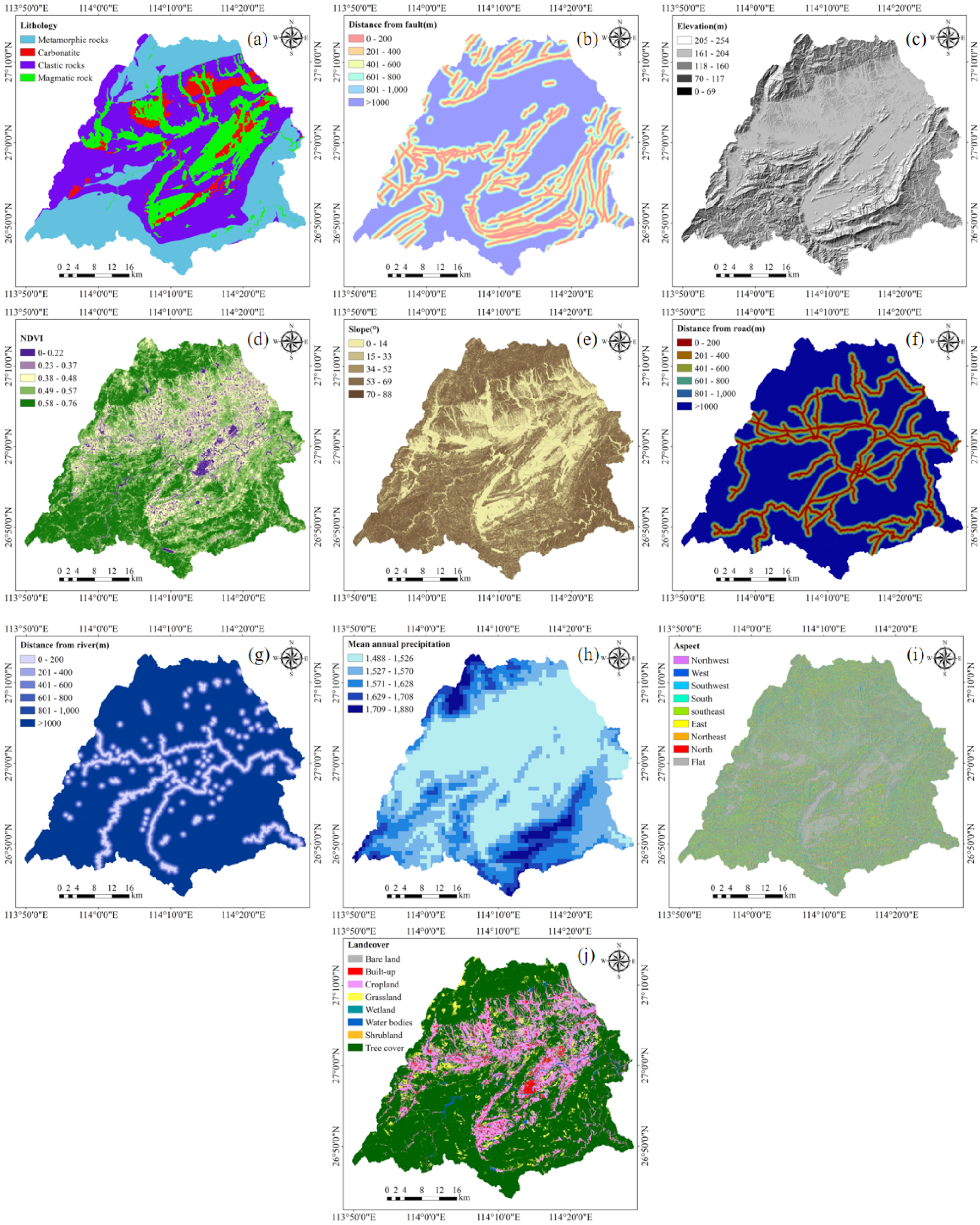
Based on ArcGIS software, elevation and slope and aspect data were extracted from the collected DEM data. The distances to faults, rivers, and roads were calculated as continuous raster layers by computing the Euclidean distance from the corresponding vector data, and the results were smoothed using the Kriging interpolation method. The NDVI was derived from Sentinel-2 imagery (with an original resolution of 10 m) and resampled to 5 m using the bicubic convolution method. It should be noted that the resampling process does not truly enhance the spatial resolution; rather, it interpolates coarser-resolution pixels into smaller units to better align spatially with other factors. Land use data were also resampled to 5 m using the Kriging spatial interpolation method. Considering that landslides in the study area are predominantly small in scale, all conditioning factors were ultimately unified to a 5 m spatial resolution to better capture local topographic features. In terms of factor classification, this study refers to the research results of Ke C et al. [37], dividing the distances to faults, rivers, and roads into 6 levels according to the intervals of [0, 200], (200, 400], (400, 600], (600, 800], (800, 1000], and (1000, +∞); the other factors were automatically divided into 5 levels using the natural break point method (Jenks natural breaks) combined with the statistical distribution characteristics of the data. This method can maximize the similarity within groups and the difference between groups, avoiding the subjectivity of the classification process, and is widely used in the research of factor classification in geoscience environments. The factor classification results are shown in Figure 2. Due to significant differences in the values of the factors, normalization is applied to all evaluation factors.

2.3. Method

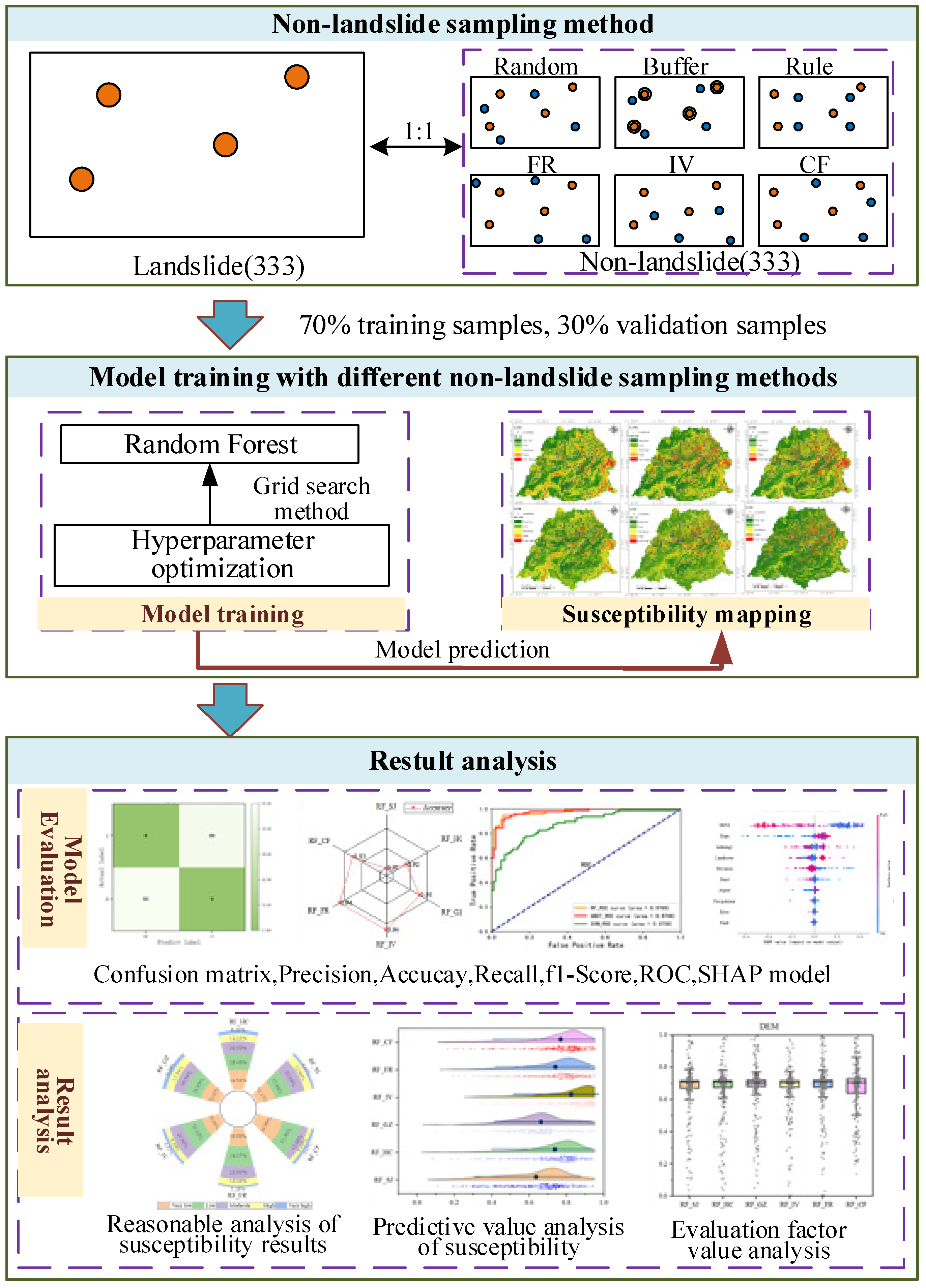
The landslide susceptibility assessment workflow is shown in Figure 3. Based on 333 landslide sample points, non-landslide sample points are selected at a 1:1 ratio. Six non-landslide sample point sampling methods—random method, buffer zone method, rule-based method, FR method, IV method, and CF method—are employed. Firstly, the sample points are divided into training and validation datasets at a 7:3 ratio. Then, based on the RF model, hyperparameter optimization is performed using grid search, and models are trained using different non-landslide sample sampling methods. Finally, precision analysis is conducted using a confusion matrix, accuracy, precision, recall, F1 score, ROC curve, and SHAP model, followed by a rationality analysis of the evaluation results to determine the optimal non-landslide sample sampling method.
The hardware environment for the training, validation, and testing process includes an Intel (R) Core (TM) i7-11700k 8-core processor (manufactured by Intel Corporation, purchased in Nanchang, Jiangxi, China), an NVIDIA GeForce RTX 3080 Ti 12 GB graphics card (manufactured by NVIDIA Corporation, purchased in Nanchang, Jiangxi, China), and 128 GB Hynix DDR4 memory (manufactured by SK Hynix Inc., purchased in Nanchang, Jiangxi, China). The software environment consists of Python 3.8, which is compiled using Jupyter Notebook (Anaconda3).

2.3.1. Sampling Method of Non-Landslide Samples

The random method randomly selects non-landslide sample points from the study area [37,50]. The buffer zone method, based on buffer zone analysis, creates a 1000 m buffer around all landslide sample points [37,51], and non-landslide sample points are then randomly selected outside the buffer zone. The rule-based distribution method constructs a grid for the study area according to the required number of non-landslide sample points. In this study, to ensure the spatial uniform distribution of non-slide sample points and to guarantee that the number of non-slide samples generated matches that of slide samples, the required number of rows and columns for the grid units within the study area range is calculated. A 23-row by 24-column grid is built, and grids outside the study area, or those extensively outside the study area, are removed. A point is randomly generated within each grid, avoiding landslide areas, and this point is used as a non-landslide sample point. The FR method involves first calculating the frequency ratios of each evaluation factor, and then summing up all the factor frequency ratios to obtain the Landslide Susceptibility Index (LSI). The natural discontinuity point method is used to divide it into five levels of prone areas: extremely low, low, medium, high, and extremely high. The resulting map of landslide LSI zoning is obtained (as shown in Formulas (1) and (4)). Then, non-landslide sample points are selected in the extremely low- or low-susceptibility zones [52,53,54]. The Information Value Model (IV) and Certainty Factor Model (CF) are similar to the FR method, where non-landslide sample points are selected from the extremely low- and low-susceptibility zones of their calculated susceptibility zoning maps [41] The calculation formulas are as follows:
F R = N i / N S i / S
I V = ln N i / N S i / S
C F = P a P s P a ( 1 P s ) , P a < P s P a P s P a ( 1 P s ) , P a P s
L S I F R = i = 1 n F R i
L S I I V = i = 1 n I V i
L S I C F = i = 1 n C F i
The formula represents the study area, “i” represents a certain type of evaluation factor. S i denotes the total area of the region classified by a specific factor, N refers to the total number of landslide in the study area, N i is the number of landslides occurring within the range classified by the factor, I represents the amount of information in the evaluation unit, and P a is the conditional probability of landslide occurrence in the factor classification data a . In practical studies, this can be represented by the ratio of the number of (or area of) landslides in factor classification a to the total area of classification a . P s indicates the ratio of the total number (or area) of in the entire study area to the total area of the study area. L S I F R , L S I I V and L S I C F represent the LSI values based on frequency ratio, information content, and coefficient of determination models, respectively. F R i , I V i , C F i represent the FR, IV, and CF values corresponding to the i-class evaluation factors.

2.3.2. Random Forest

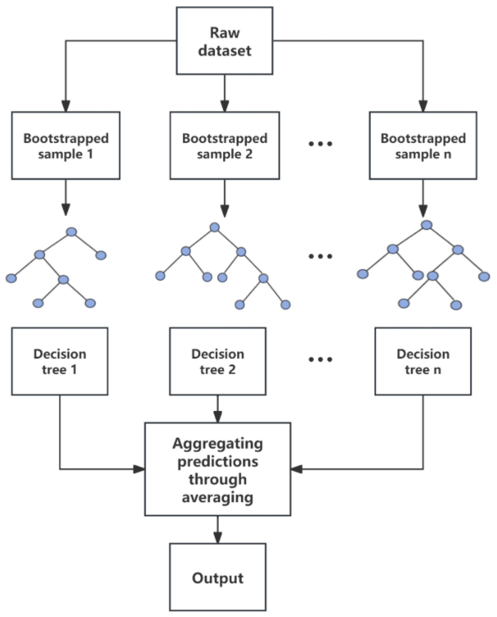
Random Forest is an ensemble learning method proposed by Leo Breiman in 2001 [55], designed to address the overfitting issue encountered by a single decision tree when handling complex data. It enhances model accuracy and robustness by combining the predictions of multiple decision trees. The core construction of Random Forest includes: using Bootstrap sampling to generate the training data for each decision tree, employing random feature selection to reduce the correlation between trees, and ultimately aggregating the predictions of all trees through voting or averaging, as shown in Figure 4. Random Forest is known for its strong resistance to overfitting, high accuracy, ability to handle large datasets, feature importance evaluation, robustness to noise and outliers, and support for parallel processing. However, a key drawback is its higher computational cost, especially when dealing with a large number of trees, which can increase both training and prediction time. Due to these advantages, it has been widely applied in various fields, particularly excelling in classification tasks. In addition, grid search is a commonly used method for hyperparameter optimization. Hyperparameters refer to the parameters that must be set before model training, such as the number of trees, maximum depth, or splitting criteria in a random forest, which significantly affect model performance. The principle of grid search is to systematically generate combinations of hyperparameters within a predefined range in a grid-like manner, train and validate the model for each parameter set, and then compare the performance (often through cross-validation) to identify the optimal parameter combination [56,57].

2.3.3. Evaluation Index of Accuracy

In this paper, accuracy, precision, recall, F1 score, and ROC curve are used to comprehensively evaluate the reliability of the machine learning model [58,59].
(1)
Confusion Matrix
The confusion matrix is commonly used to assess the performance of classification models. Through the confusion matrix, accuracy, precision, recall, and F1 score can be calculated (As shown in Table 2 and Table 3). These evaluation metrics provide a comprehensive reflection of the model’s classification effectiveness [60,61]. The detailed calculation formulas are as follows:
In this context, TP represents the number of correctly predicted landslide sample points, FP represents the number of incorrectly predicted landslide sample points, TN represents the number of correctly predicted non-landslide sample points, and FN represents the number of incorrectly predicted non-landslide sample points.
(2)
ROC Curve
This paper uses the ROC curve to evaluate the predictive performance of the susceptibility assessment model. This metric reduces the interference from different test datasets and helps assess the model’s generalization ability. Since the ROC curve itself cannot clearly distinguish the superiority of classifiers, the area under the ROC curve (Area Under the Curve, AUC) is introduced as the evaluation criterion [62,63]. The AUC is generated by calculating sensitivity (the proportion of correctly predicted landslide sample points) and specificity (the proportion of correctly predicted non-landslide sample points). The ROC curve shows specificity on the x-axis and sensitivity on the y-axis. The AUC value ranges between 0 and 1, with higher values generally indicating better predictive accuracy of the model; however, values that are too close to 1 do not necessarily imply excellent model performance, as they may indicate potential overfitting. Therefore, AUC should be interpreted in conjunction with other metrics and validation methods [64].
(3)
SHAP Model Calculation Principle
This paper adopts the SHAP (Shapley Additive Explanations) model to explain the internal workings and feature selection mechanism of the susceptibility assessment model [65,66,67]. SHAP is a game-theoretic explanation method that uses Shapley values to measure the contribution of each feature to the model’s prediction. To calculate the Shapley value, a series of feature subsets is generated to cover all possible feature combinations. For categorical features, SHAP typically treats different categories as independent features, thereby analyzing complex feature relationships. The calculation formula is as follows [41,68]:
ϕ i = S N { i } S ! ( n S 1 ) ! n ! f ( S { i } ) f ( S )
In the formula, ϕ i represents the contribution of the i-th evaluation factor, N is the total number of evaluation factors, S is the subset of predictive features, f ( S { i } ) denotes the model result containing the i-th evaluation factor, and f ( S ) represents the model result without the i-th evaluation factor. The contribution of each evaluation factor to the model’s prediction is quantified, and the sum of the Shapley values for each input feature is calculated.
f ( x ) = ϕ 0 + M i = 1 ϕ i
In the formula, f ( x ) represents the model’s prediction result for sample x ; ϕ 0 is the mean prediction for all training samples (the constant in the explanation model); ϕ i represents the contribution of the i-th evaluation factor to the model’s prediction result (the Shapley value), and M is the number of evaluation factors.

3. Results

3.1. Distribution of Non-Landslide Point Samples

The landslide susceptibility indices (LSI) derived from the FR, IV, and CF methods were uniformly classified into five levels using the Jenks natural breaks method. To evaluate the performance of these methods, the Area Under the Curve (AUC) values were calculated, thereby ensuring the reliability of the selected non-landslide samples. The results showed that the AUC values for FR, IV, and CF were 0.8120, 0.8235, and 0.8044, respectively. Although these values are lower than those obtained from the machine learning models, they still provide a meaningful reference.
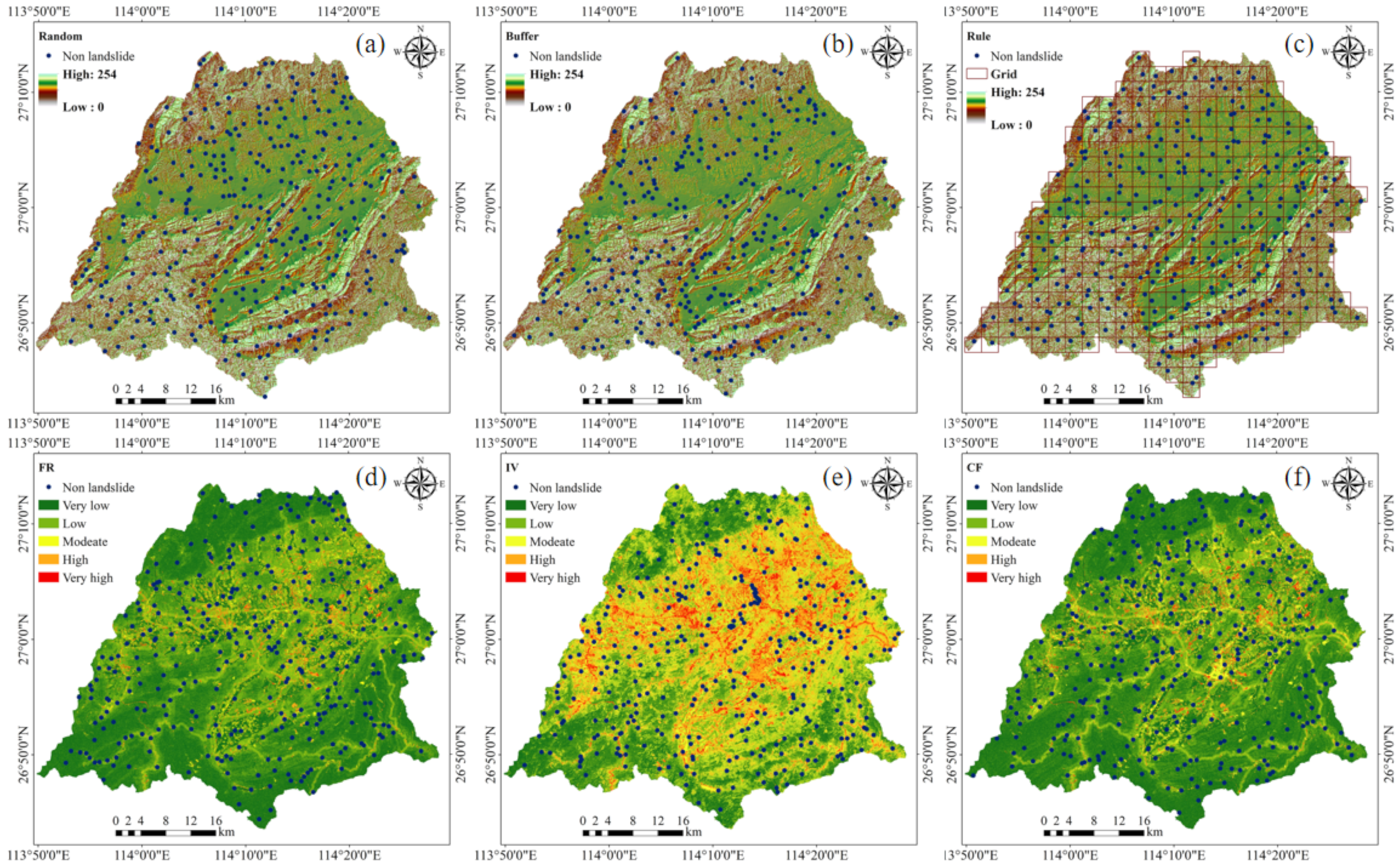
Non-landslide sample points were selected using the six methods described in Section 2.3.1, and the spatial distribution map of these points is shown in Figure 5. Figure 5a shows the randomly selected non-landslide sample points within the study area; Figure 5b represents the random selection of one non-landslide sample point within each grid; Figure 5c shows the random selection of non-landslide sample points outside the 1 km buffer zone established around landslide sample points. Additionally, the FR, IV, and CF values for each evaluation factor were calculated (Table 4), and the landslide susceptibility grid map was derived using Formulas (4)–(6). The map was classified into five levels using the natural breaks method, and non-landslide sample points were randomly selected in the very low- and low-susceptibility zones (Figure 5d–f).

3.2. Evaluation Results of Model Accuracy

This paper uses six different non-landslide sample methods for susceptibility evaluation, with a uniform random forest model (RF) for the evaluation. For ease of subsequent mapping and comparative analysis, the six non-landslide sample methods (random, rule-based, buffer, FR, IV, CF) combined with the RF model are abbreviated as RF_SJ, RF_GZ, RF_HC, RF_FR, RF_IV, and RF_CF, respectively. This paper employs the grid search method to optimize the parameters of each model. The optimal parameters of each model are shown in the Table 5.
The parameter “n_estimators” represents the number of decision trees in the forest, “max_depth” refers to the maximum depth of a single decision tree, and “min_samples_split” indicates the minimum number of samples required for further splitting of an internal node.
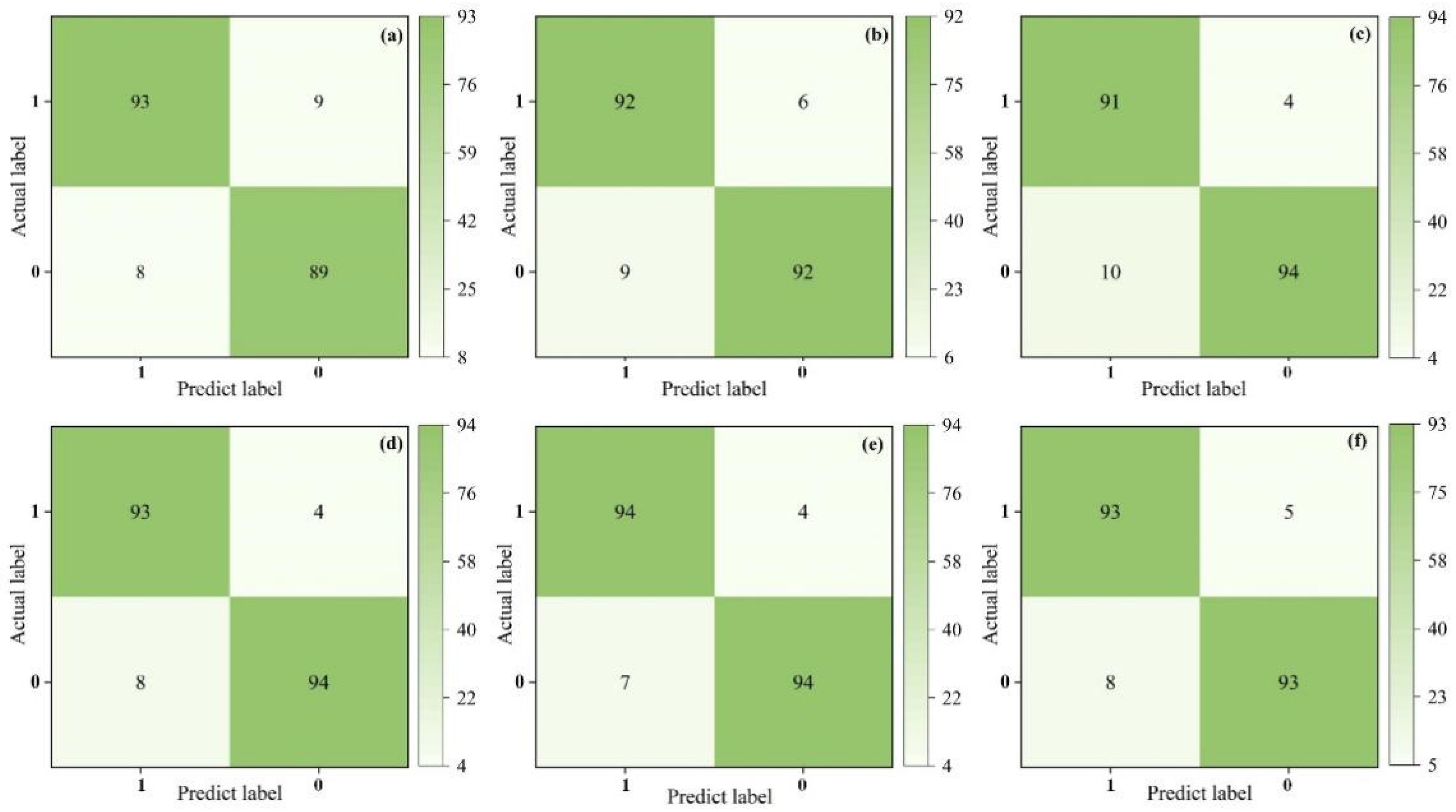
To compare the predictive performance of different non-landslide sample methods, the confusion matrix and ROC curve are used to validate the model accuracy. The confusion matrices computed with different non-landslide sample methods are shown in Figure 6. From the figure, it can be seen that for the models from RF_SJ to RF_GZ, the number of correctly classified landslide samples is 93, 92, and 91, respectively, indicating that the RF_SJ model has higher accuracy and predictive performance compared to the other two models. In contrast, for the RF_FR, RF_IV, and RF_CF models, the number of correctly classified landslide samples is 93, 94, and 93, respectively. Therefore, the lowest model accuracy and predictive performance are found in the RF_SJ model, while the RF_IV coupled model achieves the highest accuracy and predictive performance.
The accuracy, precision, recall, and F1 score metrics were calculated using the confusion matrix to quantitatively evaluate the model’s performance, with the results shown in Figure 7. From the figure, it can be observed that in terms of accuracy, the RF_SJ, RF_HC, RF_GZ, RF_IV, RF_FR, and RF_CF models have accuracy values of 0.91, 0.92, 0.93, 0.94, 0.94, and 0.93, respectively. The RF_SJ model has the lowest accuracy, indicating that the randomly selected non-landslide samples perform the worst. The RF_IV and RF_FR models have the highest accuracy, correctly predicting the proportion of landslides in actual landslide prediction. In terms of precision, the RF_IV and RF_FR models again have the highest precision, both at 0.96, which is 0.06 higher than the RF_GZ model, 0.04 higher than the RF_SJ and RF_CF models, and 0.05 higher than the RF_HC model. Based on precision, the RF_IV and RF_FR models exhibit the best predictive performance. In terms of recall, the RF_GZ, RF_CF, RF_HC, RF_IV, RF_FR, and RF_SJ models have recall values of 0.96, 0.95, 0.94, 0.93, 0.92, and 0.91, respectively. For the F1 score, the RF_IV and RF_FR models have the same F1 score of 0.94, followed by the RF_GZ and RF_CF models with an F1 score of 0.93. The lowest F1 score is observed in the RF_SJ model, with a value of only 0.91. Therefore, by comprehensively comparing accuracy, precision, recall, and F1 score, it can be concluded that the three coupled models based on statistical methods and RF have better accuracy and performance. Among them, the RF_IV model achieves the best landslide susceptibility prediction accuracy and performance, while the RF_SJ model has the worst accuracy and performance.
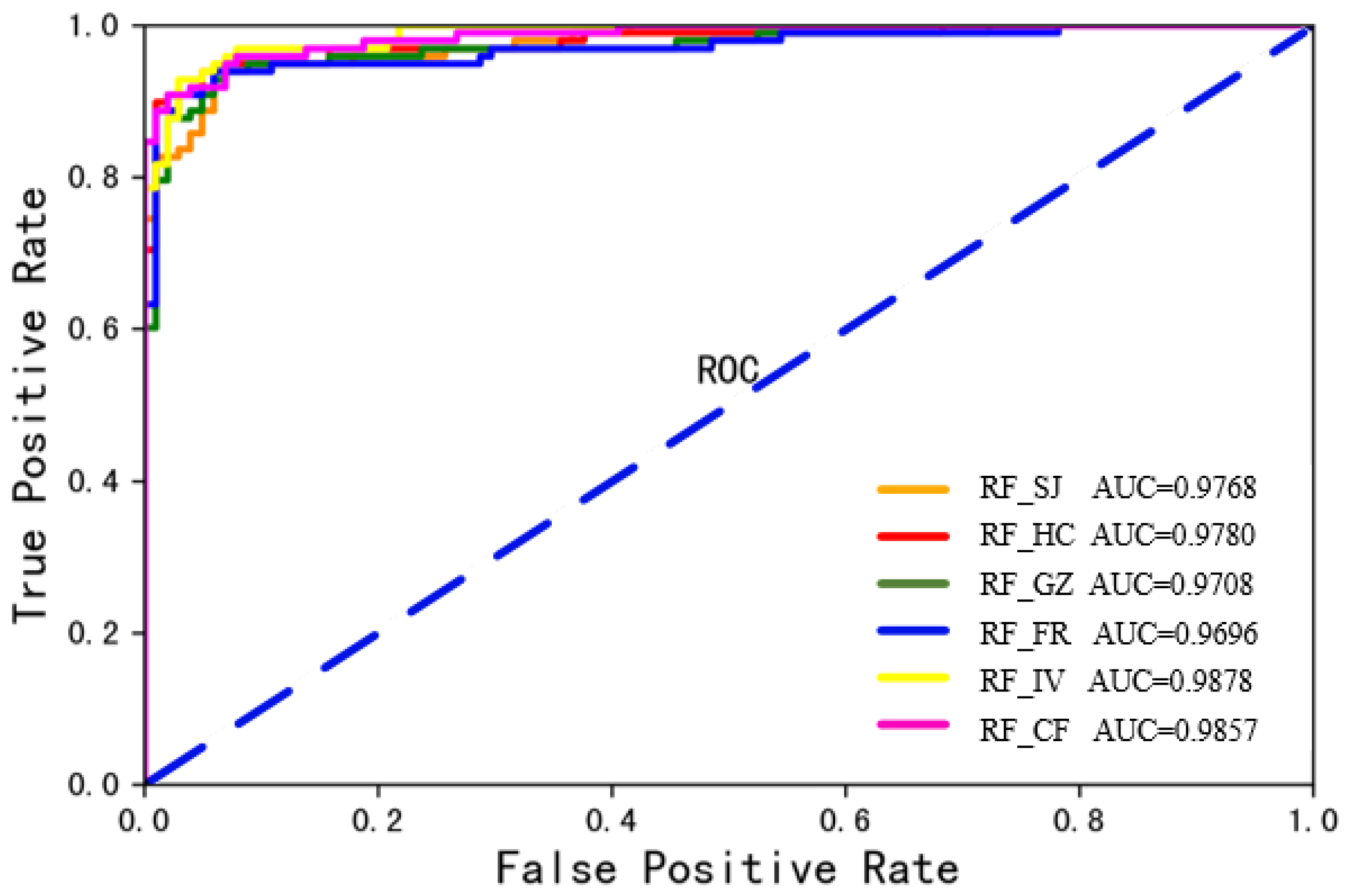
By comparing the ROC curves of the six different non-landslide sample models, it can be seen from Figure 8 that the AUC values of all six models are greater than 0.96, with relatively small differences between them. Among these, the highest AUC value is achieved by the RF_IV model, with an AUC of 0.9878, while the lowest AUC value is observed in the RF_FR model, with a value of 0.9696. In conclusion, the RF_IV model exhibits the best susceptibility prediction performance within the study area, and thus, the non-landslide sample selection based on the information content method provides the most effective susceptibility evaluation.

3.3. Contribution Analysis Results of Evaluation Factors Using the SHAP Model

To further understand the decision-making process of the landslide susceptibility model, this paper applies the SHAP model to analyze the contribution of evaluation factors. The SHAP algorithm evaluates the influence of various factors by calculating the SHAP values for each sample. In the plots, the X-axis (SHAP value) represents both the direction and magnitude of a feature’s impact on the model output: a positive value indicates that the feature increases the predicted landslide susceptibility value, thereby raising the likelihood of landslide occurrence, while a negative value indicates that the feature decreases the predicted susceptibility value, thereby reducing the likelihood of occurrence. The larger the absolute SHAP value, the greater the influence of the feature on the model output. The Y-axis represents the ranking of the importance of evaluation factors, where factors are ordered from top to bottom in decreasing order of importance. The importance is determined based on the absolute SHAP values of all samples. Additionally, the color indicates the magnitude of the evaluation factor values, with blue representing lower feature values and red representing higher feature values. The color gradient illustrates the impact of changes in feature values on the model. Each point represents a sample, and the clustering of samples reflects the distribution and impact of features [69].
Figure 9 shows the comparison of SHAP values among six different non-landslide sample models. From the figure, it can be seen that in the randomly selected non-landslide samples (Figure 9a), lithology, land use, slope, DEM, and NDVI have relatively large SHAP values, indicating that these factors significantly influence the model’s predictions. Among them, lithology has the largest SHAP value, making the greatest impact on landslide susceptibility prediction, followed by land use. The SHAP values for fault distance, river distance, and aspect are relatively small, with the smallest being fault distance, which has a SHAP value close to 0. In the non-landslide samples outside the buffer zone (Figure 9b), slope, NDVI, land use, DEM, and lithology are the key factors influencing the RF model. Land use has the largest SHAP value, while slope’s SHAP values mainly range between 0.1 and 0.2. In the rule-based selection of non-landslide samples (Figure 9c), slope, lithology, NDVI, land use, and DEM are identified as the primary influencing factors for the RF model. For non-landslide samples selected within FR, IV, and CF (Figure 9d–f), NDVI, slope, and lithology are the major influencing factors. Overall, although variations exist among the six models, slope, NDVI, lithology, land use, and elevation consistently emerge as the dominant controlling factors. Lithology plays a critical role due to the widespread presence of weathered and fractured granite, slate, and sandstone–shale, which are highly prone to failure. Steeper slopes, particularly those above 33° (Table 4), markedly increase shear stress and act as a direct driving condition for landslides. NDVI shows a negative correlation, reflecting the stabilizing role of vegetation through root reinforcement and rainfall interception, whereas sparsely vegetated slopes are more susceptible to erosion. Land use also contributes significantly, as human disturbances such as excavation and cultivation weaken slope stability. Elevation exerts a mixed effect, with mid-to-high zones experiencing greater dissection and rainfall, in contrast to the relatively stable valley deposits. By comparison, fault distance, river distance, and aspect show consistently low SHAP values across all methods, aligning with the field reality that small, scattered faults and valley-confined rivers exert limited control on slope instability.

3.4. Mapping of Susceptibility Assessment Results Based on Different Non-Landslide Samples

3.4.1. Mapping of Susceptibility Assessment

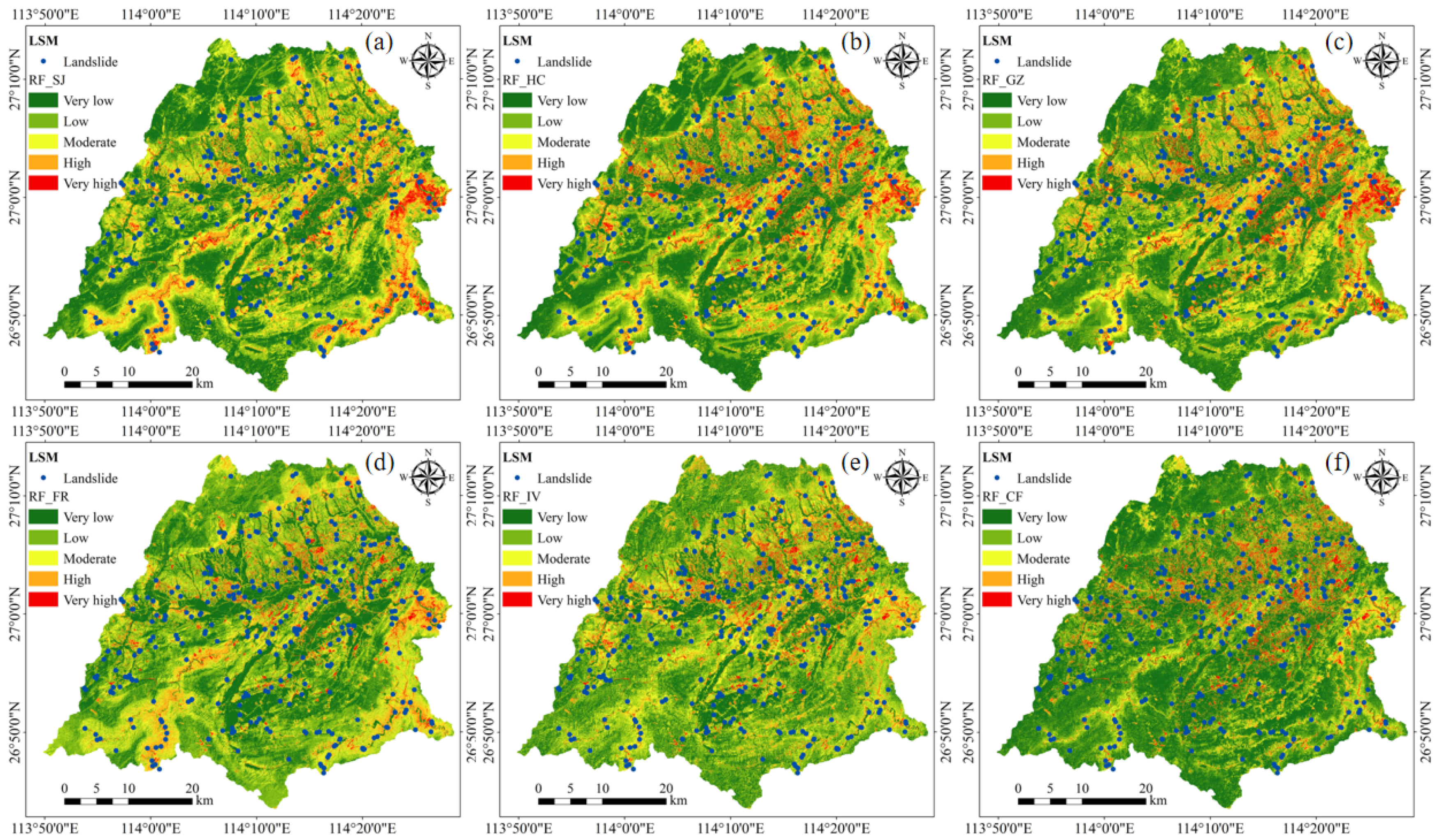
By training different non-landslide samples using the RF model, landslide susceptibility maps for the study area were generated to analyze the impact of non-landslide sample selection on the uncertainty of susceptibility results. The natural breaks method was used to classify the susceptibility results of the study area into five sensitivity levels: very low, low, medium, high, and very high. The final landslide susceptibility mapping (LSM) results are presented in Figure 10, with red zones indicating high-susceptibility areas. Analysis of the LSM for different non-landslide sample methods indicates that the landslide susceptibility evaluation results for the six non-landslide sample selection methods are generally similar, with the distribution of each sensitivity level being mostly the same, though the areas differ. Overall, the very low- and low-susceptibility areas occupy a large proportion of the total area, followed by the medium susceptibility areas. Moreover, the distribution of landslide points closely matches the LSM distribution. The very high- and high-susceptibility areas are primarily located in the eastern and central parts of the study area, where the terrain is generally steeper, and the geological structure is dominated by faults. With numerous roads present, human engineering activity is prevalent in the area. Additionally, intense residential activity involving slope cutting for housing construction is also evident. The very high- and high-susceptibility areas exhibit a trend of small area but wide and scattered distribution, similar to the distribution characteristics of landslides in the southern regions.
Field investigations show that the landslides in the study area are mainly distributed in the northeastern and central regions with relatively low vegetation coverage. The central and eastern parts of the area are mainly composed of hills and valleys. The terrain is steep and the slope is relatively large, providing topographic conditions for the sliding of slope rock and soil masses. The landslide materials are mostly rock and soil masses with weak lithology, low shear strength and prone to weathering. Rainfall infiltration softens the soil and weak structural surfaces, further reducing the stability of the slope. In addition, human engineering activities (such as the excavation of the foot of the slope in road construction) weaken the supporting force of the slope, resulting in frequent landslides along the road. The SHAP analysis of the six types of non-landslide samples in Figure 9 further reveals that slope, NDVI, lithology, land use type, elevation and road distance are the main controlling factors of landslides in the study area. The above-mentioned multi-source evidence jointly verified the rationality of the evaluation results of landslide susceptibility.

3.4.2. Analysis of Susceptibility Evaluation Results

Based on the susceptibility zoning results, quantitative statistical methods were used to analyze the area proportion, number, and frequency ratio of landslides in each susceptibility zone in detail, further testing the effectiveness of the model. The statistical results are shown in Table 6. From Table 6, it can be seen that all landslide susceptibility evaluation results were classified using the natural breaks method, but the index ranges of each classification are relatively close. In this study, the natural breaks method rather than equal interval classification was applied, because the natural breaks approach can automatically identify optimal thresholds based on the inherent distribution of the data, thereby maximizing inter-class differences and minimizing intra-class variance. This makes it more consistent with the spatial distribution characteristics of landslide susceptibility and is therefore widely adopted in geoscientific studies. For example, the index ranges for the very low-susceptibility zones of RF_SJ, RF_HC, RF_GZ, RF_FR, RF_IV, and RF_CF are [0.0, 0.14], [0.0, 0.12], [0.0, 0.12], [0.0, 0.13], [0.0, 0.14], and [0.0, 0.10] respectively, while the index ranges for the very high-susceptibility zones are (0.53, 0.97], (0.59, 1], (0.58, 0.99], (0.58, 0.99], (0.65, 0.99], and (0.62, 1] respectively. The areas of each susceptibility zone decrease progressively from low to high susceptibility, with the area of the very low-susceptibility zone accounting for about 30% of the total in most cases, with the exception of RF_CF, which accounts for 44.90%. The area proportion of the very high-susceptibility zone is less than 7%, with the highest proportion for RF_GZ at 6.24%, and the lowest for RF_FR at 3.28%. Regarding landslide numbers, all six methods show that the majority of landslides occur in the very high-susceptibility zone, with only a small number of landslides occurring in the very low- and low-susceptibility zones. A comparison of the frequency ratio reveals that in the very low-, low-, and moderate-susceptibility zones, the frequency ratio is less than 1, especially in the very low and low zones, where the frequency ratio is close to 0. In the high-susceptibility zone, the frequency ratio approaches 1. In the very high-susceptibility zone, RF_GZ exhibits the lowest frequency ratio of 11.79, while RF_FR exhibits the highest frequency ratio of 25.98. Both values exceed 1, indicating that these factors contribute positively to landslide occurrence, with RF_FR exerting a comparatively stronger influence on landslide susceptibility. The landslide susceptibility probabilities show a positive correlation with the susceptibility zone levels, gradually increasing as the susceptibility zone level increases. This further reflects the model’s susceptibility prediction results being well aligned with actual geological conditions. In the field of geology, it is generally believed that landslides are mainly concentrated in the high- and very high-susceptibility zones. By using different non-landslide sampling methods and comparing the model prediction performances, the following conclusions can be drawn: (1) The RF_SJ model predicts that 90.69% of landslides occur in the high- and very high-susceptibility zones, covering 17.13% of the total area. (2) The RF_HC model predicts that 94.89% of landslides occur in 18.47% of the corresponding area. (3) The RF_GZ model predicts that 94.89% of landslides occur in 18.47% of the corresponding area. (4) The RF_FR model predicts that 97.00% of landslides occur in 13.72% of the area. (5) The RF_CF model predicts that 95.80% of landslides occur in 11.00% of the area. (6) The RF_IV model predicts that 97.60% of landslides occur in 12.99% of the area. Thus, it is evident that the RF_IV model performs better than the other models in terms of prediction accuracy.
The rationality of the susceptibility evaluation results is mainly analyzed by examining the area percentage of each susceptibility zone and the number of landslides included in each zone. Table 6 provides a detailed statistical analysis of the landslide susceptibility results predicted by six different non-landslide sample selection methods. To better visualize the statistical results, bar charts were created for the area percentage and the number of landslides in each susceptibility zone, as shown in Figure 11. Generally, an ideal susceptibility zoning usually shows that as the susceptibility level increases, the area percentage of each susceptibility zone gradually decreases, while the number of landslides in each zone correspondingly increases. Figure 11a shows the area percentage of each susceptibility zone. From the chart, it can be observed that the prediction results from the six different non-landslide sample selection methods follow the same pattern. Figure 11b displays the number of landslide sample points included in each susceptibility zone. This also follows the trend where the number of landslide points gradually increases from low- to high-susceptibility zones, with most landslide points concentrated in the very high-susceptibility zones. As the sensitivity level increases, the area percentage gradually decreases. Therefore, the landslide susceptibility results predicted by the six different non-landslide sample selection methods are all reasonable.
However, it should be noted that in this study, the proportion of very low- and low-susceptibility zones exceeds 50%, while the proportion of high-susceptibility zones is relatively small. This may pose a potential risk of overfitting when using a 1:1 ratio of landslide to non-landslide samples [70,71]. Previous studies have demonstrated that different sample ratios (e.g., 1:1, 1:2, 1:5) can influence model performance, suggesting that future work could include a sensitivity analysis of sample ratios to validate the robustness of the results under different sampling schemes.

4. Discussion

4.1. Comparison of Different Sampling Methods for Non-Landslide Samples

When constructing a landslide susceptibility evaluation model, the selection and quality of non-landslide samples are crucial. However, the definition of non-landslide samples remains inconsistent within China. The most commonly used approach is to select regions where landslides have never occurred as non-landslide samples. Yet, this method may inadvertently include potential landslides, thereby affecting the model’s prediction accuracy [43]. This paper examines the impact of six different non-landslide sample selection methods on susceptibility evaluation results. Among them, random selection is the most commonly used method, and using the RF model on this basis yields relatively good prediction accuracy. However, this approach may result in samples that do not cover all types of areas that have never experienced landslides or may have deviations from the actual situation [36,41]. The buffer zone method can narrow the scope of non-landslide samples, but the buffer distance setting still lacks a unified standard and needs to be adjusted based on landslide characteristics [42]. The rule-based method ensures even distribution of samples but may be blindly applied and might fail to select true non-landslide areas [41]. The FR, IV, and CF methods can effectively avoid landslide regions, but the FR method has issues with capturing non-landslide terrain comprehensively. The CF method assumes that the susceptibility of landslides has a linear relationship with the evaluation factors, but in reality, the susceptibility of landslides may have a complex nonlinear relationship with the evaluation factors [42,43]. In contrast, the IV model has better ability to handle interactions between factors and does not require complex assumptions. It is particularly suitable for data-scarce or imbalanced situations, performing better in study areas with complex geological and environmental factors [72].
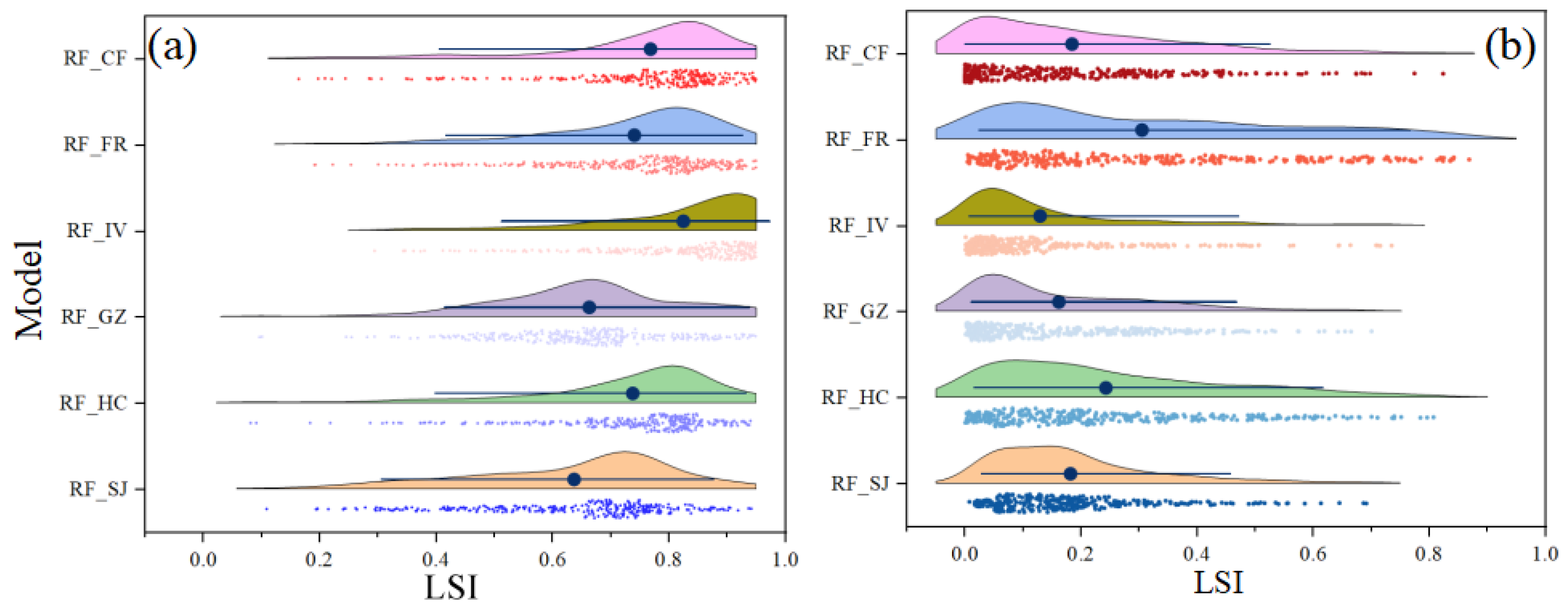
The selection of non-landslide samples requires an in-depth analysis of the unique characteristics and topography of landslide in the study area, taking multiple factors into consideration to ensure the scientific and representative nature of the samples, thus improving the accuracy of landslide susceptibility evaluation. Through cloud and rain plot analysis of landslide and non-landslide sample points (Figure 12), the study finds that the landslide sample points predicted by the RF_IV model have the highest and most concentrated values, with a median of 0.883, whereas the non-landslide sample points have the lowest prediction values, mainly concentrated below 0.18. In comparison, the prediction value distribution of other methods is more scattered, reflecting that the RF_IV model provides the highest prediction accuracy and indicating that the non-landslide samples selected by the IV method are of higher quality, significantly improving the model’s accuracy.
Taking NDVI and slope as example evaluation factors, box plots (Figure 13) were used to assess the distribution of non-landslide sample values (normalized evaluation factor values). The results show that the NDVI values of RF_CF and RF_IV models are more concentrated, while 75.38% of landslide sample points have NDVI values less than 0.37 (Table 4). Regarding slope, non-landslide sample points are mainly concentrated in low-slope areas, and the RF_IV method shows the highest concentration, contrasting sharply with the high-slope distribution of landslide sample points (Table 4). Further analysis indicates that the IV method outperforms other non-landslide sample selection approaches for two main reasons. First, it effectively addresses data imbalance. By calculating the information value, the IV method appropriately allocates sample weights, enabling the model to more accurately learn features from both classes, and its AUC value is slightly higher than those of the CF and FR models. Second, it reduces noise interference. When selecting non-landslide samples, the IV method excludes potential landslide-prone areas similar to landslide samples, thereby minimizing the impact of noisy samples on model training and enhancing the stability and reliability of model predictions. These results suggest that the non-landslide samples selected using the IV method follow more regular patterns, avoiding randomness and uncertainty, and are therefore more reliable and scientific.

4.2. Compared with Models from Other Studies

In the selection methods of non-landslide samples for landslide susceptibility evaluation, several scholars have conducted similar studies (Table 7). For example, the study by Dou et al. [42] demonstrated that the information entropy method and conditional factor method resulted in higher quality non-landslide samples and better evaluation accuracy than the buffer zone method. Zhu et al. [42] compared four non-landslide sampling methods (random method, buffer zone method, frequency ratio method, and analytic hierarchy process) and found that the frequency ratio and analytic hierarchy methods yielded higher susceptibility evaluation accuracy than the other two methods, with the highest accuracy achieved by the analytic hierarchy process. Trinh et al. [43] applied three susceptibility evaluation methods (SVM, Bayesian, and KNN) and verified that landslide samples selected using the frequency ratio method had higher quality than those selected using the analytic hierarchy process. These studies indicate that the accuracy and rationality of landslide susceptibility evaluation results are closely related to the quality of non-landslide sample selection.
Building on the aforementioned studies, this paper summarizes and improves upon previous methods by proposing six non-landslide sample selection methods and then constructs a landslide susceptibility evaluation model for the study area using random forests. The results indicate that the RF_IV model achieves the highest prediction accuracy, with an AUC value of 0.9878, while models constructed using other non-landslide sample selection methods also generally outperform those reported in previous studies. This improvement may be attributed to differences in the study area, the historical landslide samples, and the spatial resolution of evaluation factor data. In this study, the evaluation factors were processed at a 5 m spatial resolution, whereas previous studies typically used 30 m resolution data. Higher-resolution data better capture local topographic features, thereby enhancing landslide susceptibility evaluation accuracy, as also demonstrated by Yang et al. [73]. These findings provide practical guidance for policymakers to optimize landslide prevention strategies and land-use planning. The method also has transferable potential and can be applied to landslide susceptibility assessments in other mountainous regions of China or similar terrains worldwide.

5. Conclusions

This study investigates the impact of non-landslide sample selection methods on landslide susceptibility evaluation. Based on 333 landslide sample points in Yongxin County, Jiangxi Province, ten evaluation factors—including slope aspect, elevation, slope, and lithology—were selected. Six non-landslide sampling methods (random selection, buffer zone, rule-based distribution, frequency ratio, information entropy, and coefficient of determination) were employed to build susceptibility models. The Random Forest model was used for training, and model performance was quantitatively assessed using confusion matrix, accuracy, precision, recall, F1 score, and ROC curve, while the SHAP model analyzed the contribution of each factor. Results show that the choice of non-landslide samples significantly affects model performance. The findings provide practical guidance for local governments, planners, and disaster managers in landslide prevention, land-use planning, and policy-making. Moreover, the methodology and insights have transferable potential, offering reference for landslide susceptibility studies in other mountainous regions of China and similar terrain worldwide. The findings are as follows:
(1)
Among the six different non-landslide sample selection methods, the RF_IV model achieved the highest accuracy, precision, recall, and F1 score, with values of 0.94, 0.96, 0.93, and 0.94, respectively, outperforming other models. It also had the highest AUC value, 0.9878, indicating that the IV method provided the best quality non-landslide samples.
(2)
The SHAP model analysis revealed that different models have distinct decision-making mechanisms. NDVI, slope, lithology, land cover, and DEM were identified as the primary contributing factors for susceptibility evaluation, while fault distance, river distance, and slope aspect had relatively small SHAP values, indicating a minimal influence on the model.
(3)
According to the susceptibility evaluation statistics, the RF_IV model predicted that 97.60% of landslides corresponded to areas with high or very high susceptibility, covering 12.99% of the area. This indicates that most landslide sample points are located within a small area, aligning with the susceptibility results, and significantly outperforming other models.
Despite the achievements of this study, several limitations remain. First, the sample size and spatial distribution are constrained by the available landslide records and the non-landslide sample selection methods, which may affect the generalizability of the model. Second, although the evaluation factors cover geological, topographic, hydrological, and vegetation aspects, temporal factors such as rainfall were not considered, potentially limiting the model’s dynamic applicability. Future research could integrate deep learning and machine learning techniques to assess the quality of landslide and non-landslide samples, automate and refine the exclusion of invalid data, and thereby enhance overall landslide susceptibility prediction performance.

Author Contributions

Conceptualization, L.T.; Methodology, L.T.; Software, S.L. and P.L.; Validation, L.T., S.L., P.L. and M.L.; Formal analysis, L.T.; Investigation, S.L., P.L. and W.L.; Resources, L.T., M.C., M.L. and Y.M.; Data curation, L.T.; Writing—original draft, L.T.; Writing—review & editing, M.C., S.L., P.L., M.L., W.L. and Y.M.; Visualization, S.L., P.L. and W.L.; Supervision, M.C.; Project administration, M.C.; Funding acquisition, M.C. All authors have read and agreed to the published version of the manuscript.

Funding

This study was supported by the financial support from the National Natural Science Foundation of China [Grant No. 42461041].

Data Availability Statement

The original contributions presented in the study are included in the article, further inquiries can be directed to the corresponding author.

Conflicts of Interest

Authors Peng Leng, Shengwei Liu, Mei’e Liu, Wang Luo and Yaqin Mao were employed by the Jiangxi Nuclear Industry Surveying and Mapping Institute Group Co., Ltd. The remaining authors declare that the research was conducted in the absence of any commercial or financial relationships that could be construed as a potential conflict of interest.

Abbreviations

LSPLandslide susceptibility prediction.
LSILandslide susceptibility indexes.
RFRandom forest.
FRFrequency Ratio.
IVInformation Value.
CFCertainty Facto.
SJIt indicates that the non-landslide samples are randomly selected.
GZIt indicates that non-landslide samples are selected according to the rules.
HCNon-landslide samples are selected according to the buffer zone.
RF_SJ, RF_GZ, RF_HC, RF_FR, RF_IV, RF_CFIt represents a coupled model in which the random forest model is successively combined with non-landslide sample sampling using methods such as randomness, regularity, buffer zone, frequency ratio, information quantity, and deterministic coefficient.
F1-scoreIt is a balanced measure of a model’s accuracy.
ROCReceiver Operating Characteristic curve.
AUCArea Under ROC.
LSMLandslide Susceptibility Mapping.
NDVINormalized Difference Vegetation Index.
DEMDigital Elevation Model.

References

  1. Alcántara-Ayala, I.; Sassa, K. Landslide risk management: From hazard to disaster risk reduction. Landslides 2023, 20, 2031–2037. [Google Scholar] [CrossRef]
  2. Froude, M.J.; Petley, D.N. Global fatal landslide occurrence from 2004 to 2016. Nat. Hazards Earth Syst. Sci. 2018, 18, 2161–2181. [Google Scholar] [CrossRef]
  3. He, F.; Gu, L.; Wang, T.; Zhang, Z. The synthetic geo-ecological environmental evaluation of a coastal coal-mining city using spatiotemporal big data: A case study in Longkou, China. J. Clean. Prod. 2017, 142, 854–866. [Google Scholar] [CrossRef]
  4. Vakhshoori, V.; Pourghasemi, H.R.; Zare, M.; Blaschke, T. Landslide Susceptibility Mapping Using GIS-Based Data Mining Algorithms. Water 2019, 11, 2292. [Google Scholar] [CrossRef]
  5. Roodposhti, M.S.; Aryal, J.; Pradhan, B. A Novel Rule-Based Approach in Mapping Landslide Susceptibility. Sensors 2019, 19, 2274. [Google Scholar] [CrossRef]
  6. Ganesh, B.; Vincent, S.; Pathan, S. Machine learning based landslide susceptibility mapping models and GB-SAR based landslide deformation monitoring systems: Growth and evolution. Remote Sens. Appl. Soc. Environ. 2023, 29, 100905. [Google Scholar]
  7. Liu, G.; Dai, E.; Xu, X. Quantitative Assessment of Regional Debris-Flow Risk: A Case Study in Southwest China. Sustainability 2018, 10, 2223. [Google Scholar] [CrossRef]
  8. Franny, G.M.; Mauro, R.; Francesca, A. Hazard and population vulnerability analysis: A step towards landslide risk assessment. J. Mt. Sci. 2017, 14, 1241–1261. [Google Scholar] [CrossRef]
  9. Kim, S.; Lee, H. Assessment of Risk Due to Debris Flow and Its Application to a Marine Environment. Mar. Georesour. Geotechnol. 2015, 33, 7–23. [Google Scholar]
  10. Abhijit, S.P.; Sachin, S.P. Remote sensing and GIS-based landslide susceptibility mapping using LNRF method in part of Western Ghats of India. Quat. Sci. Adv. 2023, 11, 100095. [Google Scholar] [CrossRef]
  11. Lai, F.; Shao, Q.; Lin, Y. A method for the hazard assessment of regional geological disasters: A case study of the Panxi area, China. J. Spat. Sci. 2021, 66, 143–162. [Google Scholar] [CrossRef]
  12. Cao, J.S.; Qin, S.W.; Yao, J.Y. Debris flow susceptibility assessment based on information value and machine learning coupling method: From the perspective of sustainable development. Environ. Sci. Pollut. Res. 2023, 30, 87500–87516. [Google Scholar] [CrossRef] [PubMed]
  13. Tang, R.X.; Yan, E.C.; Wen, T. Comparison of Logistic Regression, Information Value, and Comprehensive Evaluating Model for Landslide Susceptibility Mapping. Sustainability. 2021, 13, 3803. [Google Scholar] [CrossRef]
  14. Ke, K.; Zhang, Y.C.; Zhang, J.Q. Risk Assessment of Earthquake-Landslide Hazard Chain Based on CF-SVM and Newmark Model-Using Changbai Mountain as an Example. Land 2023, 12, 696. [Google Scholar] [CrossRef]
  15. Huangfu, W.; Qiu, H.; Wu, W. Enhancing the Performance of Landslide Susceptibility Mapping with Frequency Ratio and Gaussian Mixture Model. Land 2024, 13, 1039. [Google Scholar] [CrossRef]
  16. Ke, C.Y.; He, S.; Qin, Y.G. Comparison of natural breaks method and frequency ratio dividing attribute intervals for landslide susceptibility mapping. Bull. Eng. Geol. Environ. 2023, 82, 384–402. [Google Scholar] [CrossRef]
  17. Topaçli, Z.K.; Ozcan, A.K.; Gokceoglu, C. Performance Comparison of Landslide Susceptibility Maps Derived from Logistic Regression and Random Forest Models in the Bolaman Basin, Türkiye. Nat. Hazards Rev. 2024, 25, 481–494. [Google Scholar] [CrossRef]
  18. Shang, H.; Su, L.X.; Chen, W. Spatial Prediction of Landslide Susceptibility Using Logistic Regression (LR), Functional Trees (FTs), and Random Subspace Functional Trees (RSFTs) for Pengyang County, China. Remote Sens. 2023, 15, 4952. [Google Scholar] [CrossRef]
  19. Huang, W.; Ding, M.; Li, Z. Landslide susceptibility mapping and dynamic response along the Sichuan-Tibet transportation corridor using deep learning algorithms. Catena 2023, 222, 106866. [Google Scholar] [CrossRef]
  20. Nam, B.H.; Park, K.; Kim, Y.J. Prediction of karst sinkhole collapse using a decision-tree (DT) classifier. Geomech. Eng. 2024, 36, 441–453. [Google Scholar]
  21. Chen, Z.; Tang, J.F.; Song, D.Q. Modeling landslide susceptibility using alternating decision tree and support vector. Terr. Atmos. Ocean. Sci. 2024, 35, 44195. [Google Scholar]
  22. Guo, Z.; Shi, Y.; Huang, F. Landslide susceptibility zonation method based on C5.0 decision tree and K-means cluster algorithms to improve the efficiency of risk management. Geosci. Front. 2021, 12, 101249. [Google Scholar] [CrossRef]
  23. Zhang, A.; Zhao, X.; Zhao, X. Comparative study of different machine learning models in landslide susceptibility assessment: A case study of Conghua District, Guangzhou, China. China Geol. 2024, 7, 104–115. [Google Scholar]
  24. Ye, C.M.; Tang, R.; Wei, R.L. Generating accurate negative samples for landslide susceptibility mapping: A combined self-organizing-map and one-class SVM method. Front. Earth Sci. 2023, 10, 4027. [Google Scholar] [CrossRef]
  25. Amatya, P.; Emberson, R.; Kirschbaum, D. Multitemporal landslide inventory and susceptibility map for the Arun River Basin, Nepal. Geosci. Data J. 2024, 11, 669–679. [Google Scholar] [CrossRef]
  26. Fan, H.D.; Lu, Y.F.; Shao, S.W. Evaluation and analysis of statistical and coupling models for highway landslide susceptibility. Geomat. Nat. Hazards Risk 2023, 14, 7612. [Google Scholar] [CrossRef]
  27. Li, X.; Cheng, J.L.; Yu, D.H. Research on landslide hazard assessment in data-deficient areas: A case study of Tumen City, China. Acta Geophys. 2023, 71, 1763–1774. [Google Scholar] [CrossRef]
  28. Wei, R.; Ye, C.; Sui, T. Combining spatial response features and machine learning classifiers for landslide susceptibility mapping. Int. J. Appl. Earth Obs. Geoinf. 2022, 107, 102681. [Google Scholar] [CrossRef]
  29. Yang, K.; Niu, R.Q.; Song, Y.X. Dynamic Hazard Assessment of Rainfall-Induced Landslides Using Gradient Boosting Decision Tree with Google Earth Engine in Three Gorges Reservoir Area, China. Water 2024, 16, 1638. [Google Scholar] [CrossRef]
  30. Saad, M.; Kamel, M.; Moftah, H. Landslide susceptibility mapping for the Red Sea Mountains: A multi-criteria decision analysis approach. J. Afr. Earth Sci. 2024, 209, 105–125. [Google Scholar]
  31. Ma, J.W.; Lei, D.Z.; Ren, Z.Y. Automated Machine Learning-Based Landslide Susceptibility Mapping for the Three Gorges Reservoir Area, China. Math. Geosci. 2024, 56, 975–1010. [Google Scholar]
  32. Shahabi, H.; Ahmadi, R.; Alizadeh, M. Landslide Susceptibility Mapping in a Mountainous Area Using Machine Learning Algorithms. Remote Sens. 2023, 15, 3112. [Google Scholar] [CrossRef]
  33. Pereira, P.; Fernandes, L.; Do Valle, R.J. Geomorphologic risk zoning to anticipate tailings dams’ hazards: A study in the Brumadinho’s mining area, Minas Gerais, Brazil. Sci. Total Environ. 2024, 912, 169136. [Google Scholar] [CrossRef]
  34. Pana, T.; Taipodia, J.; Philley, P.D. Landslide hazard vulnerability assessment using surface wave method coupled with slope stability analysis: A case study. Sādhanā Acad. Proc. Eng. Sci. 2024, 49, 12046. [Google Scholar] [CrossRef]
  35. Park, S.; Kim, J. Landslide Susceptibility Mapping Based on Random Forest and Boosted Regression Tree Models, and a Comparison of Their Performance. Appl. Sci. 2019, 9, 942. [Google Scholar] [CrossRef]
  36. Gu, T.F.; Duan, P.; Wang, M.G. Effects of non-landslide sampling strategies on machine learning models in landslide susceptibility mapping. Sci. Rep. 2024, 14, 7201. [Google Scholar] [CrossRef]
  37. Ke, C.; Sun, P.; Zhang, S. Influences of non-landslide sampling strategies on landslide susceptibility mapping: A case of Tianshui city, Northwest of China. Bull. Eng. Geol. Environ. 2025, 84, 123. [Google Scholar] [CrossRef]
  38. Chang, Z.L.; Huang, J.S.; Huang, F.M.; Bhuyan, K.; Meena, S.R.; Catani, F. Uncertainty analysis of non-landslide sample selection in landslide susceptibility prediction using slope unit-based machine learning models. Gondwana Res. 2023, 117, 307–320. [Google Scholar] [CrossRef]
  39. Zhai, S.; Sun, Y.; Lei, J. An improved information quantity method for non-landslide selection to enhance landslide susceptibility evaluation: A case study in Yongfeng, South China. Nat. Hazards 2025, 121, 11773–11797. [Google Scholar] [CrossRef]
  40. Hong, H.Y.; Wang, D.S.; Zhu, A.X. Landslide susceptibility mapping based on the reliability of landslide and non-landslide sample. Expert Syst. Appl. 2024, 243, 122933. [Google Scholar] [CrossRef]
  41. Zhu, Y.; Sun, D.; Wen, H. Considering the effect of non-landslide sample selection on landslide susceptibility assessment. Geomat. Nat. Hazards Risk 2024, 15, 392–409. [Google Scholar] [CrossRef]
  42. Dou, H.Q.; He, J.B.; Huang, S.Y. Influences of non-landslide sample selection strategies on landslide susceptibility mapping by machine learning. Geomat. Nat. Hazards Risk 2023, 14, 5719. [Google Scholar] [CrossRef]
  43. Liu, Q.; Tang, A.P.; Huang, D.L. Exploring the uncertainty of landslide susceptibility assessment caused by the number of non–landslides. Catena 2023, 227, 107109. [Google Scholar] [CrossRef]
  44. Wang, C.; Lin, Q.; Wang, L. The influences of the spatial extent selection for non-landslide samples on statistical-based landslide susceptibility modelling: A case study of Anhui Province in China. Nat. Hazards 2022, 112, 1967–1988. [Google Scholar]
  45. Zhu, Y.; Liu, S.; Yin, K. Impact of negative sampling strategies on landslide susceptibility assessment. Adv. Space Res. 2025, 76, 592–613. [Google Scholar] [CrossRef]
  46. Huang, F.; Xiong, H.; Jiang, S. Modelling landslide susceptibility prediction: A review and construction of semi-supervised imbalanced theory. Earth-Sci. Rev. 2024, 250, 104700. [Google Scholar]
  47. Jiang, W.; Li, L.; Niu, R. Impact of non-landslide sample sampling strategies and model selection on landslide susceptibility map. Appl. Sci. 2025, 15, 2132. [Google Scholar] [CrossRef]
  48. Yang, C.; Liu, L.L.; Huang, F.M.; Huang, L.; Wang, X.M. Machine learning-based landslide susceptibility assessment with optimized ratio of landslide to non-landslide samples. Gondwana Res. 2023, 123, 198–216. [Google Scholar]
  49. Yu, X.; Chen, H. Research on the influence of different sampling resolution and spatial resolution in sampling strategy on landslide susceptibility map results. Sci. Rep. 2024, 14, 1549. [Google Scholar] [CrossRef]
  50. Sun, D.L.; Gu, Q.Y.; Wen, H.J. Assessment of landslide susceptibility along mountain highways based on different machine learning algorithms and mapping units by hybrid factors screening and sample optimization. Gondwana Res. 2023, 123, 89–106. [Google Scholar]
  51. Wang, Z.; Chen, J.; Lian, Z. Influence of buffer distance on environmental geological hazard susceptibility assessment. Environ. Sci. Pollut. Res. 2024, 31, 9582–9595. [Google Scholar] [CrossRef] [PubMed]
  52. Bhandari, B.P.; Dhakal, S.; Tsou, C. Assessing the Prediction Accuracy of Frequency Ratio, Weight of Evidence, Shannon Entropy, and Information Value Methods for Landslide Susceptibility in the Siwalik Hills of Nepal. Sustainability 2024, 16, 2092. [Google Scholar] [CrossRef]
  53. Bharadwaj, D.; Sarkar, R. Landslide Susceptibility Mapping Using Probabilistic Frequency Ratio and Shannon Entropy for Chamoli, Uttarakhand Himalayas. Iran. J. Sci. Technol.-Trans. Civ. Eng. 2024, 48, 377–395. [Google Scholar] [CrossRef]
  54. Ahmad, M.S.; MonaLisa Khan, S. Comparative analysis of analytical hierarchy process (AHP) and frequency ratio (FR) models for landslide susceptibility mapping in Reshun, NW Pakistan. Kuwait J. Sci. 2023, 50, 387–398. [Google Scholar] [CrossRef]
  55. Breiman, L. Random forests. Mach. Learn. 2001, 45, 5–32. [Google Scholar] [CrossRef]
  56. Lin, Q.; Zhang, Z.H.; Yang, Z.H. Co-seismic landslides susceptibility evaluation of Bayesian random forest considering InSAR deformation: A case study of the Luding Ms6.8 earthquake. Geomat. Nat. Hazards Risk 2024, 15, 238–253. [Google Scholar] [CrossRef]
  57. Wen, H.; Zhao, S.Y.; Liang, Y.H. Landslide development and susceptibility along the Yunling-Yanjing segment of the Lancang River using grid and slope units. Nat. Hazards 2024, 120, 6149–6168. [Google Scholar] [CrossRef]
  58. Wang, P.; Deng, H.W.; Liu, Y. GIS-based landslide susceptibility zoning using a coupled model: A case study in Badong County, China. Environ. Sci. Pollut. Res. 2024, 31, 6213–6231. [Google Scholar] [CrossRef]
  59. Nath, N.K.; Gautam, V.K.; Pande, C.B. Development of landslide susceptibility maps of Tripura, India using GIS and analytical hierarchy process (AHP). Environ. Sci. Pollut. Res. 2024, 31, 7481–7497. [Google Scholar] [CrossRef]
  60. Yang, L.; Cui, Y.; Xu, C. Application of coupling physics–based model TRIGRS with random forest in rainfall-induced landslide-susceptibility assessment. Landslides 2024, 21, 2179–2193. [Google Scholar] [CrossRef]
  61. Yao, J.M.; Yao, X.; Zhao, Z. Performance comparison of landslide susceptibility mapping under multiple machine-learning based models considering InSAR deformation: A case study of the upper Jinsha River. Geomat. Nat. Hazards Risk 2023, 14, 2212833. [Google Scholar] [CrossRef]
  62. Zhao, Y.; Huang, Z.; Wei, Z.L. Assessment of earthquake-triggered landslide susceptibility considering coseismic ground deformation. Front. Earth Sci. 2023, 10, 3975. [Google Scholar] [CrossRef]
  63. Martinello, C.; Mercurio, C.; Cappadonia, C. Using Public Landslide Inventories for Landslide Susceptibility Assessment at the Basin Scale: Application to the Torto River Basin (Central-Northern Sicily, Italy). Appl. Sci. 2023, 13, 9449. [Google Scholar] [CrossRef]
  64. Zhang, Y.B.; Xu, P.Y.; Liu, J. Comparison of LR, 5-CV SVM, GA SVM, and PSO SVM for landslide susceptibility assessment in Tibetan Plateau area, China. J. Mt. Sci. 2023, 20, 979–995. [Google Scholar] [CrossRef]
  65. Dang, K.B.; Nguyen, C.Q.; Tran, Q.C. Comparison between U-shaped structural deep learning models to detect landslide. Sci. Total Environ. 2024, 912, 169113. [Google Scholar] [CrossRef] [PubMed]
  66. Lv, J.C.; Zhang, R.; Shama, A. Exploring the spatial patterns of landslide susceptibility assessment using interpretable Shapley method: Mechanisms of landslide formation in the Sichuan-Tibet region. J. Environ. Manag. 2024, 366, 121921. [Google Scholar] [CrossRef]
  67. Al-Najjar, H.A.H.; Pradhan, B.; Beydoun, G. A novel method using explainable artificial intelligence (XAI)-based Shapley Additive Explanations for spatial landslide prediction using Time-Series SAR dataset. Gondwana Res. 2023, 123, 107–124. [Google Scholar] [CrossRef]
  68. Liu, X.M.; Su, P.C.; Li, Y. Spatial distribution of landslide shape induced by Luding Ms6.8 earthquake, Sichuan, China: Case study of the Moxi Town. Landslides 2023, 20, 1667–1678. [Google Scholar] [CrossRef]
  69. Sun, D.L.; Ding, Y.K.; Wen, H.J. SHAP-PDP hybrid interpretation of decision-making mechanism of machine learning-based landslide susceptibility mapping: A case study at Wushan District, China. Egypt. J. Remote Sens. Space Sci. 2024, 27, 508–523. [Google Scholar] [CrossRef]
  70. Rabby, Y.W.; Li, Y.; Hilafu, H. An objective absence data sampling method for landslide susceptibility mapping. Sci. Rep. 2023, 13, 1740. [Google Scholar] [CrossRef]
  71. Tien, B.D.; Tuan, T.A.; Hoang, N.D.; Thanh, N.Q.; Nguyen, D.B.; Liem, N.V.; Pradhan, B. Spatial prediction of rainfall-induced landslides for the Lao Cai area (Vietnam) using a hybrid intelligent approach of least squares support vector machines inference model and artificial bee colony optimization. Landslides 2017, 14, 447–458. [Google Scholar] [CrossRef]
  72. Xu, W.; Cui, Y.L.; Wang, J.Z. Landslide susceptibility zoning with five data models and performance comparison in Liangshan Prefecture, China. Front. Earth Sci. 2024, 12, 1417671. [Google Scholar] [CrossRef]
  73. Yang, S.; Li, D.; Sun, Y. Effect of landslide spatial representation and raster resolution on the landslide susceptibility assessment. Environ. Earth Sci. 2024, 83, 132. [Google Scholar] [CrossRef]
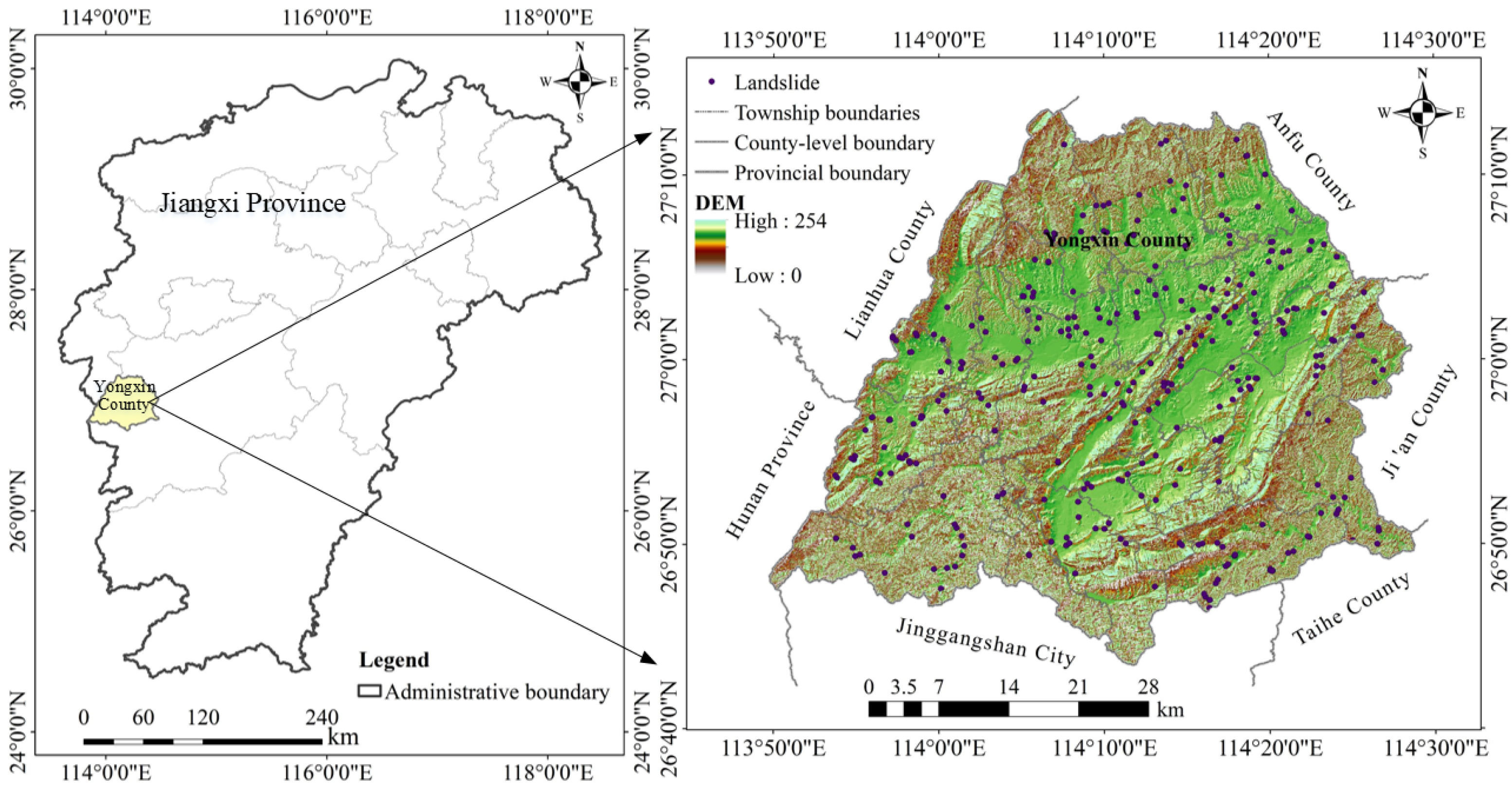
Figure 1. Study area location and spatial distribution map of landslide samples (DEM is SRTM3 Version 4).
Land 14 02059 g001
Figure 2. Landslide characteristic factors ((a) lithology, (b) distance from the fault, (c) elevation, (d) NDVI, (e) slope, (f) distance from the road, (g) distance from the river, (h) mean annual precipitation, (i) aspect, (j) landcover).
Land 14 02059 g002
Figure 3. The technical process for evaluating magnetic sensitivity based on different non-slide samples.
Land 14 02059 g003
Figure 4. The schematic diagram of the Random Forest algorithm. The blue circle symbols in the figure represent nodes.
Land 14 02059 g004
Figure 5. Selection of non-landslide sample points by different methods ((a) Random selection method, (b) Buffer selection method, (c) Rule selection method, (d) Frequency ratio selection, (e) Information selection method, (f) Determination coefficient selection method).
Land 14 02059 g005
Figure 6. Confusion matrix ((a) RF_SJ, (b) RF_HC, (c) RF_GZ, (d) RF_FR, (e) FR_IV, (f) RF_CF).
Land 14 02059 g006
Figure 7. Model evaluation indicators ((a) accuracy, (b) Precision, (c) Recall, (d) F1-score).
Land 14 02059 g007
Figure 8. ROC curve.
Land 14 02059 g008
Figure 9. SHAP of different non-landslide samples ((a) RF_SJ, (b) RF_HC, (c) RF_GZ, (d) RF_FR, (e) RF_IV, (f) RF_CF).
Land 14 02059 g009
Figure 10. Results of landslide susceptibility zoning based on different negative samples ((a) RF_SJ, (b) RF_HC, (c) RF_GZ, (d) RF_FR, (e) RF_IV, (f) RF_CF).
Land 14 02059 g010
Figure 11. Characteristic analysis of susceptibility results of different non-landslide sample models ((a) area percentage of susceptibility zones; (b) percentage of hidden landslide points in each zone).
Land 14 02059 g011
Figure 12. Cloud and rain maps based on the predicted values of landslide susceptibility using different sampling methods ((a) landslide sample sites; (b) non-landslide sample sites). The colors in the figure represent different classification models, while the points denote the predicted probability values for landslide and non-landslide samples, respectively.
Land 14 02059 g012
Figure 13. The box plot of the non-landslide sample is based on the slope normalization value and the NDVI normalization value ((a) NDVI; (b) Slope). The colors in the figure represent different classification models. The points indicate the values of non-landslide samples in the NDVI and slope spaces.
Land 14 02059 g013
Table 1. The main data used in this study.
NumberDataIntroductionSourcePurposeCoordinate System
1Sentinel-2 dataSentinel-2 Level-2A multispectral imagery (with a 10 m spatial resolution raster)European Space Agency website (https://earth.esa.int/eogateway/catalog)used for extracting NDVI data and constructing landslide characteristic factorsWorld Geodetic System 1984 (WGS84)
2Land use data10 m spatial resolution rasterAnalysis of landslide characteristic factors
3Meteorological data1 km spatial resolution rasterhttps://gpm.nasa.govUsed for extracting the characteristic factor of average annual rainfall
4LithologyPolygonal vector dataYongxin County Natural Resources BureauLandslide characteristic factorChina Geodetic Coordinate System 2000
51:50,000 Geological Hazard Risk Survey Results Text, VectorYongxin County Natural Resources BureauAnalyze the historical landslide characteristics of the study area
6Faultlinear vector dataYongxin County Natural Resources BureauConstruct landslide characteristic factors by converting to raster imagery through Euclidean distance calculation.
7Riverlinear vector dataYongxin County Natural Resources Bureau
8Roadlinear vector dataYongxin County Natural Resources Bureau
9DEM5 m spatial resolution rasterYongxin County Natural Resources BureauExtract landslide characteristic factors such as elevation, slope, and aspect.
Table 2. Confusion matrix.
//Prediction Result
Actual situationclassPositiveNegative
PositiveTPFN
NegativeFPTN
Table 3. Model evaluation index system.
NumberEvaluation SystemComputing Formula
1Accuracy A C C = T P + T N T P + T N + F P + F N
2Precision P R E = T P T P + F P
3Recall R E C = T P T P + F N
4F1-score f 1 = 2 × P R E × R E C P R E + R E C
Table 4. Statistical analysis results of susceptibility of each evaluation factor.
Evaluation FactorGrading IntervalNumber of LandslidesFRIVCF
lithologymetamorphic rock770.6806 −0.3848 −0.3186
carbonatite542.6100 0.9594 2.0793
clasolite1741.2714 0.2401 0.2560
magmatite280.4494 −0.8000 −0.6741
Fault distance
(m)
(0, 200]731.6140 0.4787 0.2838
(200, 400]431.0967 0.0923 0.6513
(400, 600]351.0281 0.0277 −0.0344
(600, 800]190.6419 −0.4434 −0.6041
(800, 1000]271.0949 0.0907 0.0998
>10001360.8486 −0.1641 −0.1354
Elevation (m)(0, 69]230.9598 −0.0411 −0.0949
(69, 117]390.9214 −0.0818 −0.0019
(117, 160]731.3954 0.3332 0.7391
(160, 204]1260.8404 −0.1739 −0.2004
(204, 254]721.1169 0.1105 −0.0972
Slope
(°)
(0, 14]130.1529 −1.8779 −0.8865
(14, 33]470.9222 −0.0810 −0.2071
(33, 52]1162.0657 0.7255 0.9495
(52, 69]1241.8448 0.6124 1.1963
(69, 88]330.4481 −0.8027 −0.6488
aspecthorizon00.0000 0.0000 −1.0000
north00.0000 0.0000 −1.0000
northeast40.1457 −1.9264 −0.9466
east300.7571 −0.2782 −0.5145
southeast631.2811 0.2477 0.2944
south1012.6549 0.9764 2.0951
southwest782.8607 1.0511 2.6100
west421.0997 0.0950 −0.2732
northwest150.3284 −1.1134 −0.8962
Annual rainfall
(mm)
(1488, 1526]2371.4638 0.3811 0.4430
(1526, 1570]640.7610 −0.2731 −0.1876
(1570, 1628]230.4509 −0.7965 −0.4684
(1628, 1708]70.2822 −1.2652 −0.8740
(1708, 1880]20.1789 −1.7210 −0.9157
River distance
(m)
(0, 200]421.9600 0.6730 1.0349
(200, 400]281.4682 0.3840 0.5975
(400, 600]281.3604 0.3078 1.0491
(600, 800]311.4584 0.3774 0.5194
(800, 1000]150.7119 −0.3398 −0.4167
>10001890.8232 −0.1946 −0.2498
NDVI(0, 0.22]312.4309 0.8883 4.1690
(0.22, 0.37]2209.3440 2.2347 8.3501
(0.37, 0.48]580.8229 −0.1949 −0.5237
(0.48, 0.57]230.1875 −1.6739 −0.8962
(0.57, 0.78]10.0097 −4.6402 −0.9933
Road distance
(m)
(0, 200]953.0577 1.1177 2.7311
(200, 400]341.2211 0.1998 0.6002
(400, 600]250.9852 −0.0149 −0.3121
(600, 800]301.2969 0.2600 0.2874
(800, 1000]170.8087 −0.2123 −0.1707
>10001320.6453 −0.4381 −0.4724
Land coverwoodland920.3918 −0.9370 −0.7857
bush00.0000 0.0000 −1.0000
water10.3625 −1.0149 −0.4500
herbaceous wetland00.0000 0.0000 −1.0000
grassland211.1928 0.1763 0.8575
cultivated land140.2530 −1.3744 −0.8391
built-up area151.4231 0.3528 −0.3006
bare land or sparse vegetation19016.3083 2.7917 18.9321
Table 5. Optimal parameter table for each model.
Modelmax_depthmin_samples_splitn_estimators
RF_SJ78150
RF_HC64200
RF_GZ68150
RF_FR84150
RF_IV98250
RF_CF84200
Table 6. Statistical table of landslide hazard zones in different non-landslide samples.
Non-Landslide SamplesSusceptibility ClassificationIndex RangeArea/km2Area ProportionNumber of LandslidesLandslide ProportionFrequency Ratio
RF_SJVery Low[0, 0.14]672.3131.17%10.30%0.01
Low(0.14, 0.24]600.8627.86%51.50%0.05
Moderate(0.24, 0.36]514.0423.84%257.51%0.31
High(0.36, 0.53]279.5912.96%5616.82%1.30
Very High(0.53, 0.97]89.794.16%24673.87%17.74
RF_HCVery Low[0, 0.12]701.8432.54%20.60%0.02
Low(0.12, 0.25]614.3128.49%20.60%0.02
Moderate(0.25, 0.40]442.1820.50%133.90%0.19
High(0.40, 0.59]265.9612.33%339.91%0.80
Very High(0.59, 1]132.296.13%28384.98%13.85
RF_GZVery Low[0, 0.12]691.2632.05%20.60%0.02
Low(0.12, 0.26]621.7028.83%20.60%0.02
Moderate(0.26, 0.4]421.4619.54%92.70%0.14
High(0.4, 0.58]287.6013.34%7522.52%1.69
Very High(0.58, 0.99]134.576.24%24573.57%11.79
RF_FRVery Low[0, 0.13]666.3630.90%00.00%0.00
Low(0.13, 0.24]741.2934.37%30.90%0.03
Moderate(0.24, 0.37]453.0721.01%72.10%0.10
High(0.37, 0.58]225.0710.44%3911.71%1.12
Very High(0.58, 0.99]70.803.28%28485.29%25.98
RF_IVVery Low[0, 0.14]645.8429.95%00.00%0.00
Low(0.14, 0.27]759.4535.22%00.00%0.00
Moderate(0.27, 0.42]471.0921.84%82.40%0.11
High(0.42, 0.65]183.048.49%309.01%1.06
Very High(0.65, 0.99]97.174.51%29588.59%19.66
RF_CFVery Low[0, 0.1]968.2144.90%00.00%0.00
Low(0.1, 0.22]679.4231.50%30.90%0.03
Moderate(0.22, 0.39]271.6412.60%113.30%0.26
High(0.39, 0.62]132.836.16%329.61%1.56
Very High(0.62, 1]104.494.85%28786.19%17.79
Table 7. Comparison of model prediction accuracy in different non-landslide point selection strategies (ROC).
SourceModelNon-Landslide SampleAUC
Dou et al. [42]Logistics regressionBuffer zone method (600 m)0.936
Buffer zone method (900 m)0.95
Buffer zone method (1200 m)0.954
Buffer zone method (1500 m)0.946
Condition factor method0.991
Information value model0.997
Artificial neural networksBuffer zone method (600 m)0.942
Buffer zone method (900 m)0.952
Buffer zone method (1200 m)0.956
Buffer zone method (1500 m)0.946
Condition factor method0.989
Information value model0.995
Zhu et al. [41]Random ForestDistrict-wide random selection method0.7483
Buffer method0.777
Frequency ratio method0.857
Analytic hierarchy process0.9164
XGBoostDistrict-wide random selection method0.7553
Buffer method0.7619
Frequency ratio method0.8668
Analytic hierarchy process0.9217
Trinh et al. [43]SVMFrequency ratio method0.969
Analytic hierarchy process0.963
BayesianFrequency ratio method0.87
Analytic hierarchy process0.817
KNNFrequency ratio method0.896
Analytic hierarchy process0.86
This studyRandom Forestrandom selection method0.9768
Buffer method0.978
Regular distribution method0.9708
Frequency ratio method0.9696
Information value method0.9878
Certainty factor method0.9857
Disclaimer/Publisher’s Note: The statements, opinions and data contained in all publications are solely those of the individual author(s) and contributor(s) and not of MDPI and/or the editor(s). MDPI and/or the editor(s) disclaim responsibility for any injury to people or property resulting from any ideas, methods, instructions or products referred to in the content.