Enhancing Drought Forecast Accuracy Through Informer Model Optimization

Abstract

As droughts become more frequent due to climate change and shifts in land use, enhancing the accuracy of drought prediction is becoming crucial for informed land and water resource management. This study employed the Informer model to forecast drought and conducted a comparative analysis with Autoregressive Integrated Moving Average (ARIMA), long short-term memory (LSTM), and Convolutional Neural Network (CNN) models. The findings indicate that the Informer model outperforms the other three models in terms of drought forecasting accuracy across all time scales. Nevertheless, the predictive capacity of the Informer model remains suboptimal when it comes to short-term intervals. Aiming at the problem of drought forecasting accuracy in a short time scale, this study proposed a drought forecasting model named VMD-JAYA-Informer based on Variational Mode Decomposition (VMD) and the JAVA optimization algorithm to improve the Informer model. This study conducted a comparative analysis of VMD-JAYA-ARIMA, VMD-JAYA-LSTM, VMD-JAYA-CNN, and VMD-JAYA-Informer drought prediction models. The performance of these models was evaluated using the root mean square error (RMSE), Nash–Sutcliffe efficiency coefficient (NSE), and Mean Absolute Error (MAE). The VMD-JAYA-Informer model’s forecast for the 1-month SPEI significantly surpasses that of alternative models and demonstrates a robust agreement with the actual data. Simultaneously, the model exhibits equally optimal forecasting performance across different time scales. In order to validate the VMD-JAYA-Informer model, four meteorological stations in the Songliao River Basin were chosen at random. The validation results demonstrate that VMD-JAYA-Informer outperforms the Informer model in terms of prediction accuracy on the 1-month time scale (NSE values of 0.8663, 0.8765, 0.8822, and 0.8416, respectively). Additionally, the model outperforms Informer in terms of prediction performance on other time scales, further demonstrating its generalizability and excellence in drought prediction on shorter time scales.

1. Introduction

Drought is a multifaceted meteorological phenomenon that has an impact on agriculture, economy, ecosystems, and various other aspects [1]. Over the past few decades, particularly since the 1990s, drought has become increasingly severe in most parts of the world. Central and northeastern regions have experienced noticeable drought trends, with some areas experiencing a yearly increase in drought coverage of 3.72%, surpassing the area of humid regions [2]. Mishra et al. 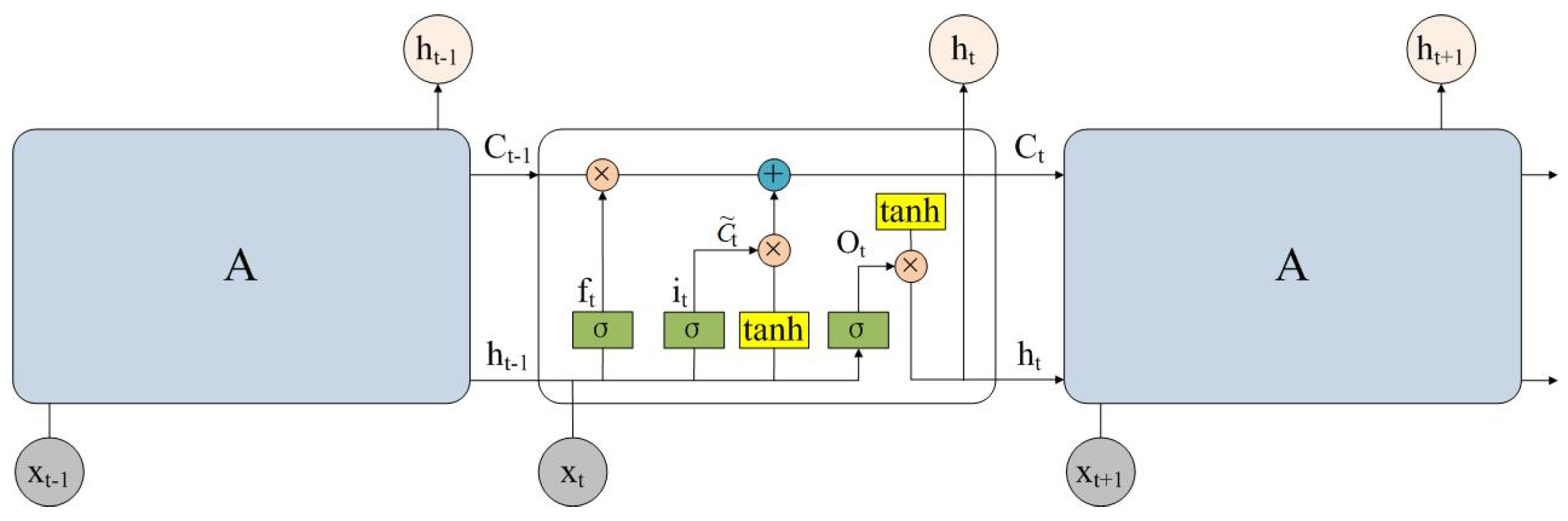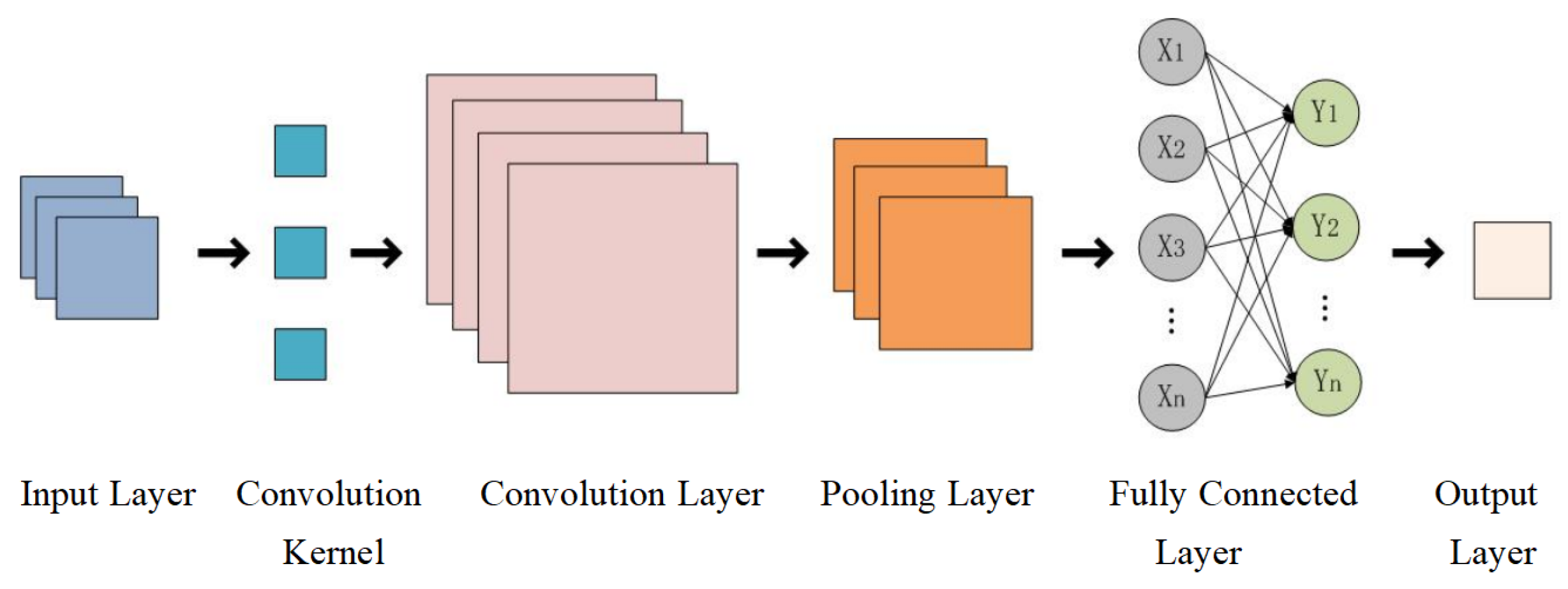identified four distinct drought categories: meteorological, agricultural, hydrological, and socio-economic [3,4]. Drought presents significant challenges to ecosystems, agriculture, and economies, necessitating research to concentrate on prediction, assessment, and risk management. Traditional forecasting methods, such as ARIMA and hydrometeorological models, leverage historical data to identify drought patterns; however, they often fail to accurately capture multidimensional non-linear data structures. The advent of artificial intelligence offers transformative advances for drought prediction, with deep learning models such as LSTM, CNN, and Informer adept at extracting intricate spatiotemporal features from diverse data sources, thus markedly improving predictive accuracy. Despite these advancements, AI-based forecasting faces critical challenges, including its reliance on extensive datasets, limitations in predicting short-term and extreme drought events, and the need for more effective multi-source data integration and model optimization. Addressing these limitations in future research is imperative to improve the accuracy of drought prediction and provide scientifically robust information to support disaster prevention and mitigation efforts. This research aims to predict drought using the Informer model, emphasizing reduction in data noise and errors to enhance prediction accuracy and efficiency. Through the refinement of the model architecture and parameter optimization, this study sought to enhance the model’s capacity to capture critical drought characteristics, ultimately providing a more precise and effective tool for drought early warning and risk management.

Prior studies typically have employed a drought index for the accurate measurement of regional drought. This index is extensively utilized for assessing and analyzing drought conditions or its spatiotemporal attributes [5,6,7]. Commonly utilized drought metrics used in studies are the Z index [8,9], Meteorological Drought Composite Index (CI), Palmer Drought Severity Index (PDSI), Standardized Precipitation Index (SPI), and Standardized Precipitation–Evapotranspiration Index (SPEI). The Palmer Drought Severity Index (PDSI) is a meteorological drought measure introduced by Palmer in 1965. It is used to analyze regional water balance by distinguishing between dry and wet periods [10]. Nevertheless, the PDSI calculation heavily relies on meteorological station data at a specific location, which greatly hampers its capacity to evaluate drought conditions across different areas. The index is inadequate for regionalizing drought and is ineffective in monitoring short-term drought across various climate regions [11]. The SPI utilizes long-term monthly precipitation data within a specific range and incorporates various time scales to measure the excess or deficiency in precipitation. This allows for the identification of drought and wet periods [12,13,14,15], as well as the determination of drought severity and duration in a particular region [1]. The SPI is determined by analyzing long-term precipitation data for a specific location. The calculation process is straightforward and can be applied to various climate conditions. However, it does not take into account the impact of temperature [16], wind speed, or other meteorological factors on evapotranspiration. Therefore, it is not suitable for analyzing the impact of climate change on evapotranspiration. The SPEI, a novel drought index introduced by Vicente-Serrano et al. in 2010, aims to overcome the constraints of the aforementioned drought indices [1]. SPEI data comprise time series information that displays various temporal scales. Hence, we used the SPEI drought index in this study.

Drought forecasting is crucial in meteorology and plays a pivotal role in preventing, mitigating, and monitoring drought risks [17]. Drought is a crucial concern in climate change and the management of water resources. Accurately predicting when and how droughts will occur is essential for agriculture, water resource planning, and disaster management [18]. Forecasting approaches for time series data play a crucial role in predicting droughts [19]. Drought forecasting methods utilize mathematical models to predict the occurrence and intensity of future droughts using historical data and meteorological indicators. There are two main types of drought forecasting methods: statistical methods and machine learning methods. Mi et al. employed an ARIMA model, LSTM model, improved LSTM model (ILSTM), and ILSTM model with additional convolutional layers (CLSTM) to forecast forthcoming drought conditions in eight specific areas of China. The findings indicated that the CLSTM reduces the root mean square error by 0.09∼0.33, making it more appropriate for short-term regional drought and climate prediction [20]. In their study on drought forecasting in the Talegan watershed, Tehran province, Iran, Nikbakht et al. discovered that the application of Support Vector Machines (SVMs) yielded more precise predictions during spring and fall [21]. Over the past decade, hybrid models have been utilized to forecast various types of droughts [22]. Ding et al. developed a Complementary Ensemble Empirical Mode Decomposition (CEEMD)-ARIMA model and a CEEMD-LSTM model to forecast drought in the Xinjiang region. The findings indicated that the CEEMD-ARIMA model achieved the highest accuracy in forecasting, and the hybrid model outperformed the individual models in accuracy across all time scales. However, there was still a lower accuracy in forecasting at shorter time scales [23]. Xu et al. integrated the advantages of ARIMA and CEEMD to predict regional droughts in China. They discovered that the combined model yielded superior results compared to using a single model. However, the accuracy of short-term predictions remained relatively poor [24]. Xu et al. conducted a comparative analysis of various forecasting models, including ARIMA, support vector regression (SVR), LSTM, ARIMA-SVR, least square SVR (LS-SVR), and ARIMA-LSTM, to predict the Standardized Precipitation–Evapotranspiration Index (SPEI) in China. The results indicated that the hybrid model had a higher accuracy in forecasting long-term SPEI, but a lower accuracy in forecasting short-term SPEI. Additionally, the ARIMA-LSTM model exhibited the highest accuracy in predicting the SPEI on the 6-, 12-, and 24-month scales, suggesting its suitability for long-term drought forecasting in China [25]. Zhang et al. employed various forecasting models, including ARIMA, random forest (RF), recurrent neural network (RNN), LSTM, and convolutional long short-term memory (ConvLSTM), to predict short-term meteorological droughts. The study revealed that ConvLSTM effectively captures spatiotemporal information and outperforms other models in short-term drought forecasting. 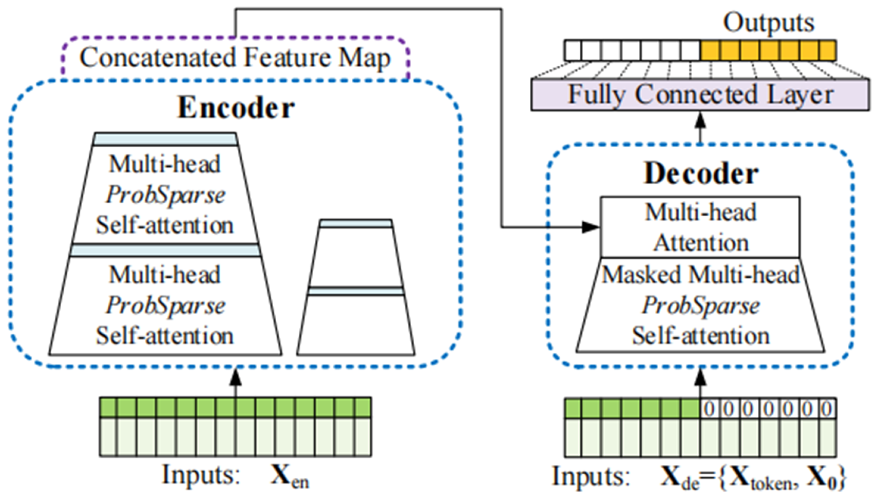Specifically, ConvLSTM exhibited high accuracy in forecasting droughts within a time frame of 1–5 days [26]. Shang et al. employed the Informer model to predict droughts in the Yangtze River Basin. The findings indicated that the Informer model outperforms LSTM and ARIMA in terms of forecasting accuracy. Nonetheless, despite some advancements in forecasting short-term droughts, the general precision of the predictions continues to be inadequate [27].

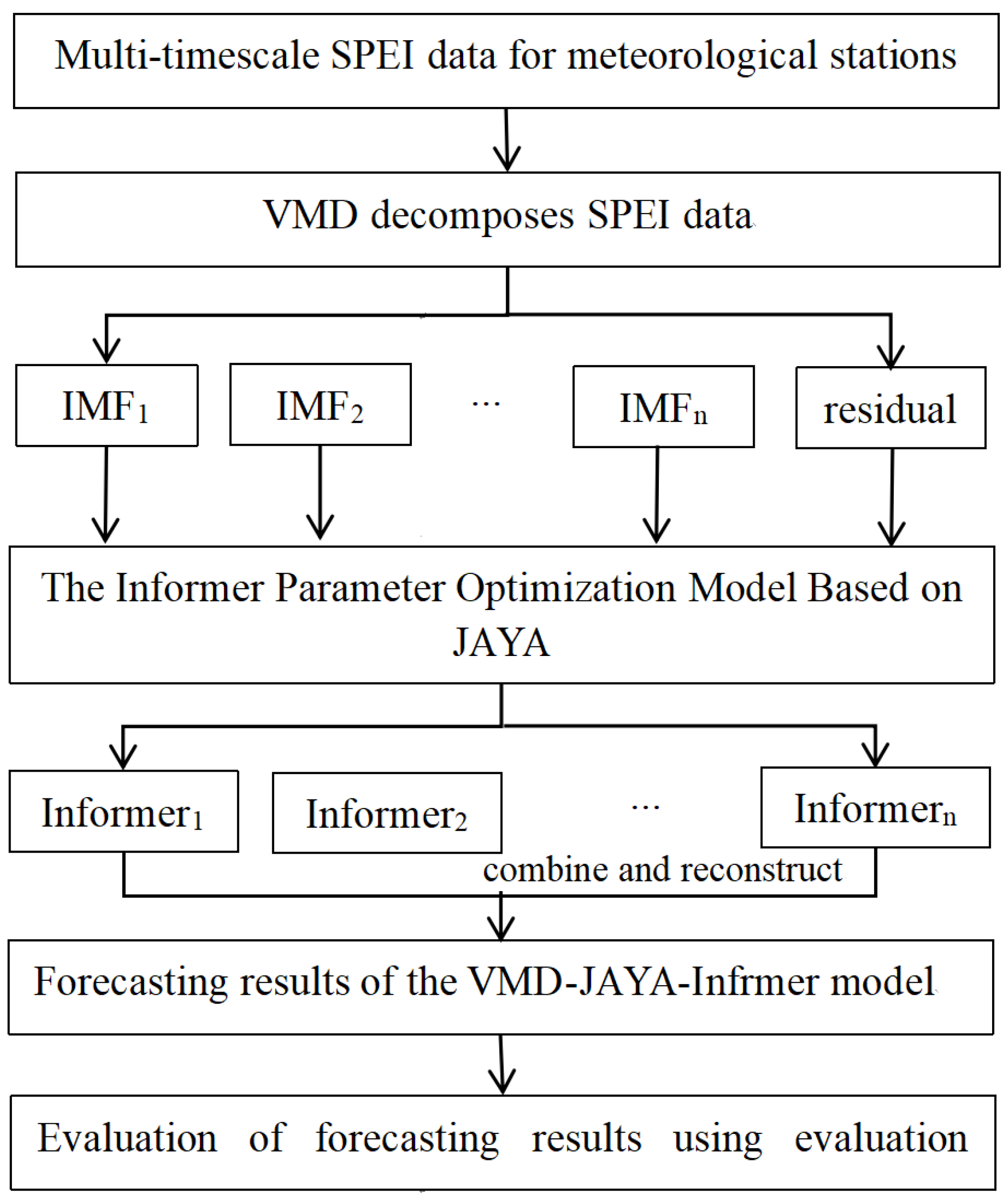
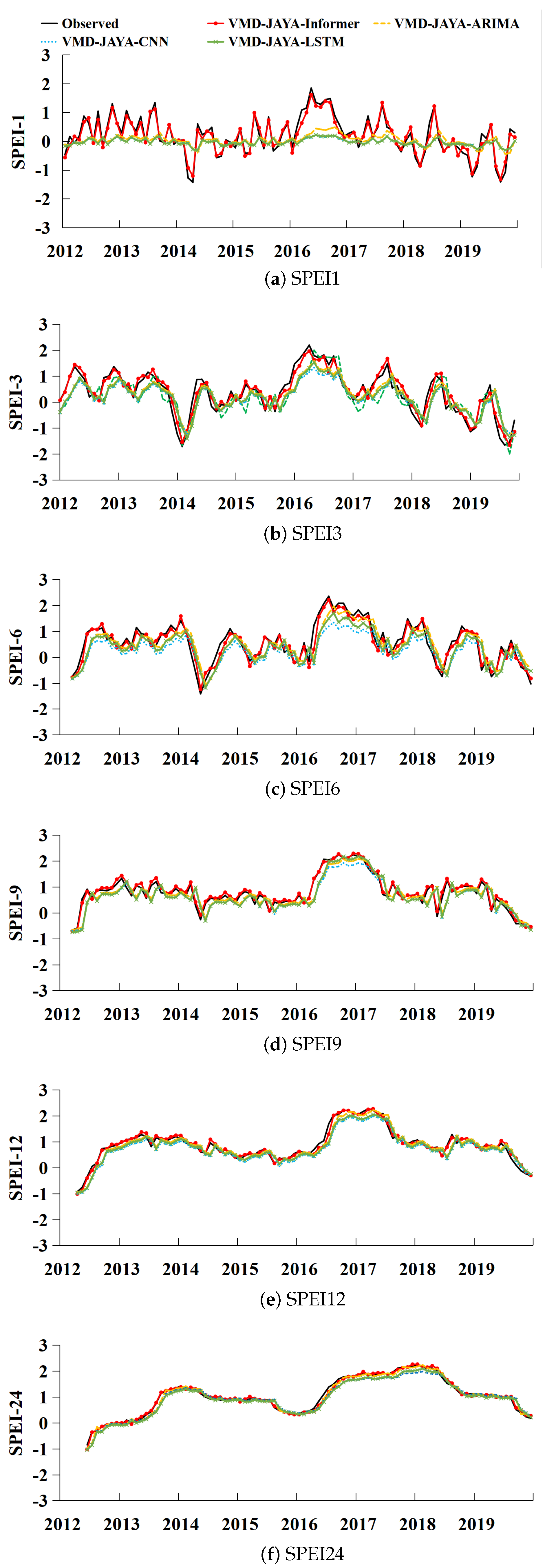
This work addresses the issue of low accuracy in predicting droughts on a short time scale, based on the scientific background provided above. While the Informer model excels at long-term forecasting, its accuracy in short-term forecasting can be influenced by factors such as excessive noise, seasonality, and periodicity. This study aims to enhance short-term forecasting by concentrating on the Songliao River Basin and integrating Variational Mode Decomposition (VMD) with the Jaya algorithm (JAYA) to improve the Informer model. The resulting model is referred to as VMD-JAYA-Informer. When comparing the predictions of VMD-JAYA-Informer with those of VMD-JAYA-LSTM, VMD-JAYA-ARIMA, and VMD-JAYA-CNN, the VMD-JAYA-Informer algorithm consistently exhibits superior accuracy in forecasting SPEI across all time scales. In this study, the SPEI data from four randomly chosen meteorological stations in the Songliao River Basin were verified.

2. Materials and Methods

2.1. Study Area

The Songliao River Basin is located in northeastern China. The basin’s climate is defined by its unique and varied topography, leading to a complex and diverse ecosystem. The spring and winter seasons are dry and cold, while the summer and fall are warm and rainy. There are noticeable variations in precipitation and temperature throughout the year, which are influenced by both seasonal changes and geographic factors. The Basin experiences an average annual temperature ranging from 1 to 5 °C. The map of the study area is shown in Figure 1.

2.2. Data Source

The meteorological data for 1980–2019 utilized in this work were obtained from the China Meteorological Science Data Sharing Service (https://www.data.cma.cn/) (accessed on 6 February 2023). In order to maintain the accuracy, consistency, and uniformity of the meteorological data, we omitted years and stations that had more than 5% of missing observations. The meteorological variables consisted of latitude, altitude (m), average wind speed (m/s), average precipitation (mm), sunshine hours (h), maximum temperature (°C), minimum temperature (°C), and average temperature (°C). The drought classification criteria of the SPEI are presented in

Table 1. Drought classification based on SPEI.

Level	Type	SPEI
1	No drought	$SPEI\ge -0.5$
2	Mild drought	$-1.0\le SPEI<-0.5$
3	Moderate drought	$-1.5\le SPEI<-1.0$
4	Severe drought	$-2.0\le SPEI<-1.5$
5	Extreme drought	$SPEI\le -2.0$

.

2.3. Methods

2.3.1. Informer

Vaswani et al. introduced the Transformer model, which utilizes a self-attention mechanism. The model is composed of an encoder–decoder structure that operates in a step-by-step manner. It incorporates a multi-head attention mechanism and a feed-forward neural network [28]. Zhou et al. introduced a model named Informer, which enhances the Transformer model [29]. Figure 2 illustrates the difference between the Informer and the self-attention mechanism in the Transformer network topology. The Informer encoder includes a multi-group multi-head, probabilistic sparse self-attention mechanism and a self-attention distilling operation [30]. The Informer’s encoder structure reduces the time dimension of the input data sequence for each layer by minimizing the cascade layers [31]. This method reduces the unnecessary computation and duplication of data storage, theoretically attaining O(LlogL). The idea is illustrated in Figure 3. The decoder architecture of the Informer produces outcomes in a single step, addressing the issue of delayed forecasting and thereby improving forecasting efficacy.

2.3.2. VMD

Dragomiretskiy and Zosso introduced VMD in 2014 as a novel variational technique for signal decomposition [32]. MD effectively decomposes the signal frequency range by taking into account the frequency domain features of the deconstructed signal, resulting in the generation of several Intrinsic Mode Functions (IMFs). The IMF is generally concentrated around its central frequency, with each IMF exhibiting an AM-FM signal [33]. The IMF formula is as follows:

$$u_k\left(t\right)=A_k\left(t\right)cos\left({\varphi }_k\left(t\right)\right),$$

(1)

where $A_k\left(t\right)$ denotes the instantaneous amplitude of $u_k\left(t\right)$, ${\varphi }_k\left(t\right)$ denotes the instantaneous phase of $u_k\left(t\right)$, and ${\varphi }_k\left(t\right)$ is a non-decreasing function.

VMD requires four parameters to be defined in advance: the modal number K, the modal bandwidth control parameter (or quadratic penalty term) $\alpha$, the noise tolerance $\tau$, and the convergence criteria tolerance $\epsilon$. The VMD method can effectively break down the signal into its primary frequency components by selecting an appropriate number of modal K [34]. Despite VMD having a strong theoretical basis and superior decomposition capabilities, parameters such as K and $\alpha$, which greatly impact VMD, are still determined based on empirical knowledge.

2.3.3. JAYA

JAYA is a population-based optimization technique, introduced by Rao in 2015 [35]. It is a very efficient algorithm specifically developed to address continuous optimization problems. It is both straightforward and robust, making it a formidable tool for achieving global optimization. The JAYA algorithm employs both optimal and worst solutions to derive a novel solution. A salient characteristic of the JAYA algorithm is its parameter-free nature, indicating that in its standard implementation, there is no requirement to establish conventional parameters (such as crossover rate, mutation rate, etc.). The fundamental idea of the JAYA algorithm is to directly guide the search process toward an optimal solution, adjusting the search direction based on the performance of the individuals [35].

2.3.4. VMD-JAYA-Informer

The VMD-JAYA-Informer model, which combines VMD, JAYA, and Informer, is introduced in this work. The principle framework of VMD-JAYA-Informer is shown in Figure 4 The JAYA method serves as an optimization engine for parameter optimization and the spatial search of the Informer model. The JAYA algorithm utilizes iterative optimization [35] to determine the optimal parameters that improve the forecasting accuracy of the Informer model on SPEI data. VMD-JAYA-Informer enhances the precision and consistency of time series data forecasting by leveraging the decomposition functionality of VMD, the optimization capabilities of JAYA, and the forecasting capabilities of the Informer. VMD-JAYA-Informer is a powerful tool that enhances the accuracy and stability of time series data forecasting. This model accomplishes this by integrating the decomposition abilities of VMD, the optimization proficiency of JAYA, and the forecasting capacity of Informer. This tool is particularly ideal for analyzing and forecasting complex time series.

Initially, the SPEI data are decomposed using VMD, a technique that breaks down the SPEI into several IMFs, where each IMF represents a distinct frequency pattern. Furthermore, the JAYA-Informer model is utilized to train and predict the deconstructed feature data from the VMD, resulting in an improved accuracy and dependability in forecasting SPEI time series. Ultimately, the modal components obtained from the forecasting process are reconfigured to restore the original state of the forecasted results.

The reconstructed data can closely approximate the original signal with a negligible margin of error. This means that the model successfully captures the distinctive features and patterns of the SPEI time series during the decomposition and forecasting procedure, suggesting the VMD-JAYA-Informer model’s high accuracy and forecasting power.

2.3.5. LSTM

In 1997, Hochrieter and Schmidhuber introduced a modified neural network model called LSTM, which is built upon the RNN [36]. The LSTM is a network model, depicted in Figure 5. It consists of four interconnected layers arranged in a chain structure. These layers are intended to influence and engage with one another via a logical function. The oblivion gate $f_t$, in the context of the hidden state $h_{t-1}$, determines which information should be reset based on the input time sequence $x_t$ at the current time t. It also determines which information should be stored in the cell. Afterward, the two-part input gate determines which new information should be added to the current cell using the sigmoid function. The tanh function is utilized to generate a fresh candidate state, in which the previous cell’s state $C_{t-1}$ is modified to the state $C_t$ in comparison to the candidate value $\widetilde{C_t}$. The blue rectangular box labeled “A” indicates an LSTM module or cell. The outcome derived from the past two procedures is utilized as the current state of the unit at the present moment in time. LSTM utilizes bidirectional information transfer and incorporates both forward and backward propagation.

2.3.6. ARIMA

ARIMA is frequently utilized to represent various time series models through parameter simplifications, thereby incorporating numerous exponential smoothing methods [37]. ARIMA is limited by the assumption of linear correlation between time series, making it unsuitable for analyzing non-linear data [38]. The modeling process necessitates numerous intrinsic parameters, resulting in computational complexity and prolonged computation period. This results in an inefficient forecasting process.

2.3.7. CNN

The CNN introduced by LeCun can be classified into 1D-CNN, 2D-CNN, and 3D-CNN based on the dimensions of the input data [39]. Convolution is a distinctive advantage of CNNs compared to traditional neural networks. It involves performing convolution operations on the input data during model training and error transfer. This process enables local connectivity and weight value sharing [40,41]. The schematic representation of its main structure can be seen in Figure 6.

2.3.8. Evaluation Metrics

This research utilizes the Nash–Sutcliffe efficiency coefficient (NSE), root mean square error (RMSE), and Mean Absolute Error (MAE) to assess the predictive capability of the model. As the value of the NSE approaches 1, it signifies a stronger alignment between the model and the data. The root mean square error (RMSE) is a numerical measure that falls within the range of ($-\infty$, 1). A smaller RMSE indicates a higher level of accuracy in the forecasting approach. The MAE is a metric that quantifies the average discrepancy between observed and anticipated values. The formulae utilized to compute the aforementioned metrics are displayed below:

$$\begin{array}{cc}\hfill & \mathrm{RMSE}=\sqrt{{\displaystyle \frac{1}{N}}\sum _{i=1}^N{(y_i-{\tilde{y}}_i)}^2}\hfill \end{array}$$

(2)

$$\begin{array}{cc}\hfill & \mathrm{NSE}=1-{\displaystyle \frac{{\sum }_{i=1}^N{(y_i-{\tilde{y}}_i)}^2}{{\sum }_{i=1}^N{(y_i-\overline{y})}^2}}\hfill \end{array}$$

(3)

$$\begin{array}{cc}\hfill & \mathrm{MAE}={\displaystyle \frac{1}{N}}\sum _{i=1}^N\left|y_i-{\tilde{y}}_i\right|\hfill \end{array}$$

(4)

where $y_i$ indicates the actual value; $\tilde{y}$ indicates the forecasted value; $\overline{y}$ represents the average value of $y_i$, and N indicates the total value of $y_i$.

2.3.9. Frequency of Drought

This study examined the Songliao River Basin’s drought frequency from 1980 to 2019 on annual and seasonal scales. The following is the formula for the drought frequency:

$$F_i={\displaystyle \frac{w}{W}}\times 100\%$$

(5)

where $F_i$ is drought frequency at station i (%), w is the number of droughts in the time series, and W is the total number of time series.

3. Results

3.1. Spatial Distribution of Drought Frequency

Figure 7 displays the geographical pattern of drought frequency in the Songliao River Basin, both on the annual basis and during different seasons. Figure 7e shows that the occurrence of drought on an annual scale varies between 30.78% and 35.85%. The regions with a higher drought frequency are mostly located in the western and southeastern parts of the Songliao River Basin. The analysis of drought frequency at the seasonal scale, as shown in Figure 7a–d, reveals that the occurrence of drought in spring ranges from 28.75% to 33.55%. The areas with a high drought frequency are mostly located in the western and northern regions of the Songliao River Basin. The occurrence of drought in summer is more frequent compared to in other seasons, primarily due to elevated temperatures, where the frequency of drought ranges from 31.60% to 36.30%, with areas experiencing high drought frequency in the western and eastern regions of the Songliao River Basin. In autumn, the frequency of drought varies from 27.11% to 33.90%, with a significant concentration of high-frequency droughts in the southwestern, southern, and eastern regions of the basin. The occurrence rate of drought during winter varies from 30.19% to 35.77%, with the region exhibiting the second highest frequency, surpassed only by autumn. This region is predominantly located in the southern and eastern sectors.

3.2. Evaluating Model’s Forecasting Performance

3.2.1. Drought Forecasting Based on Deep Learning Models

For the experiment, the main parameters involved in the model and their values are shown in

Table 2. LSTM, ARIMA, CNN and Informer Model parameters.

Model	Parameter	Parameter Value
LSTM	Epochs	50
	Batch Size	64
	Activation Function	RELU
	Loss Function	MSE
	Optimizer	Adma
ARIMA	Autoregressive Order (p)	1
	Differencing Order (d)	0
	Moving Average Order (q)	1
CNN	Convolution Kernel Size	1
	Number of Convolutional Layers	4
	Number of Pooling Layers	2
	Epochs	50
	Batch Size	64
	Activation Function	RELU
	Loss Function	MSE
	Optimizer	Adma
Informer	Input Sequence Length of Encoder (seq_len)	3
	Start Token Length of Decoder (Label_len)	1
	Encoder Input Size (enc_in)	16
	Decoder Input Size (dec_in)	8
	Dimension of Model (d_model)	512

. The parameter values were predominantly established according to the existing literature [11,12,13,15,29] and experimental results, whereas other parameters utilize the default values.

This study used the SPEI data from 1980 to 2011 at various time scales for the training set. We employed ARIMA, LSTM, CNN, and Informer to predict the SPEI values of the Songliao River Basin from 2012 to 2020. The forecasting results for each model are visualized in Figure 8. The Informer model exhibited enhanced accuracy in aligning predicted SPEI values with actual values and effectively capturing variations in SPEI values, surpassing the performance of the ARIMA, LSTM, and CNN models. The projected Standardized Precipitation–Evapotranspiration Index (SPEI) from the ARIMA, LSTM, and CNN models exhibited significant discrepancies from the actual values over a 1-month interval. Among these three models, the LSTM model demonstrated a notably weak predictive power. When predicting SPEI3, SPEI6, SPEI9, SPEI12, and SPEI24, the discrepancies between the forecasted and the actual SPEI values decreased as the time scales increased. The Informer model generates predicted SPEI values that are nearest to the actual values, succeeded by the ARIMA model. The LSTM and CNN models performed comparatively less accurately. Figure 8 clearly demonstrates that all four models performed poorly in predicting SPEI1 data. This can be attributed to the shorter time scale, frequent oscillations, rapid changes, and the significant influence of meteorological factors on SPEI values. Consequently, a more sophisticated model is required for accurately forecasting SPEI1.This research conducted a comparative analysis of the prediction performance of the ARIMA, LSTM, CNN, and Informer models using three assessment metrics: NSE, RMSE, and MAE. The results of this analysis are presented in

Table 3. The statistical criteria of the ARIMA, CNN, LSTM, and Informer models.

SPEI Series	Model	NSE	RMSE	MAE
SPEI1	ARIMA	−0.0181	0.9416	0.7468
	CNN	−0.0388	0.8927	0.7684
	LSTM	−0.1438	0.9846	0.7892
	Informer	0.1542	0.8583	0.6964
SPEI3	ARIMA	0.5086	0.7127	0.6024
	CNN	0.4217	0.6719	0.6494
	LSTM	0.4589	0.7443	0.6316
	Informer	0.5503	0.6818	0.5639
SPEI6	ARIMA	0.5180	0.6787	0.5335
	CNN	0.4351	0.6259	0.5236
	LSTM	0.4450	0.7043	0.5750
	Informer	0.5787	0.6216	0.4751
SPEI9	ARIMA	0.5718	0.5235	0.3503
	CNN	0.5309	0.4342	0.4149
	LSTM	0.4778	0.5339	0.3657
	Informer	0.6050	0.5053	0.3074
SPEI12	ARIMA	0.8325	0.2999	0.1979
	CNN	0.8200	0.2820	0.2257
	LSTM	0.8226	0.3111	0.2173
	Informer	0.8571	0.2785	0.1703
SPEI24	ARIMA	0.9276	0.1845	0.1140
	CNN	0.9009	0.1699	0.1356
	LSTM	0.8537	0.2948	0.2214
	Informer	0.9395	0.1690	0.1080

. For the ARIMA, LSTM, and CNN models, the NSE was negative, the RMSE was greater than 0.86, and the MAE was higher than 0.7 at the 1-month time period. In contrast, the Informer model had an NSE value of 0.1542, an RMSE of 0.8583, and an MAE of 0.6964. The RMSE and MAE of the ARIMA, LSTM, CNN, and Informer models decreased as the time scale increased. Conversely, the NSE exhibited the reverse tendency. This fact suggests that the forecasting accuracy of these four models improves as the time scale increases. Through a comparison of the experimental data, the Informer model demonstrates superior forecasting performance compared to ARIMA, LSTM, and CNN across all time scales. This suggests that the ARIMA, LSTM, and CNN models exhibit inferior prediction accuracy due to inherent limitations in their network structures. The Informer model markedly improves the predictive accuracy of the SPEI and adeptly resolves the challenge of insufficiently capturing the relationship between input and output time series data in long-term forecasts, a problem exacerbated by prolonged time scales.

3.2.2. Decomposition of VMD for SPEI

Constructing the VMD algorithm typically requires determining four parameters, namely, the Number of Modes (K), Penalization Factor ($\alpha$), Noise Tolerance ($\tau$), and Convergence Criterion Tolerance ($\epsilon$). Compared to K, $\alpha$, $\tau$, and $\epsilon$ have less impact on the decomposition effect of SPEI sequences and are usually using their default values [42]. When the K value is smaller, the VMD algorithm is in an under-decomposition state, and the main frequency signal contained in the SPEI series cannot be fully decomposed. Nevertheless, selecting a substantial value for K results in the central frequencies of neighboring modal components being closer together, potentially resulting in modal repetition or increased noise generation. Tang et al. calculated the IMFs’ central frequencies obtained for a given range of K values, which resulted in appropriate K values. This paper uses SPEI1 data as an example, and

Table 4. The center frequency corresponding to the IMF produced by different values of K.

K	Center Frequencies/Hz
	IMF1	IMF2	IMF3	IMF4	IMF5	IMF6	IMF7
4	69.9	11.4	6	3.3
5	243.9	47.2	22	12	9
6	322.6	62.9	29.6	20.7	15.2	11.5
7	163.9	33.3	16.1	11.4	8.2	6.8	5.8

shows the IMFs’ central frequencies generated with the K values within the established range.

From Table 4, when $K=7$, the central frequencies of IMF6 and IMF7 are similar, indicating that the decomposition of SPEI data by VMD might be in an over-decomposed state. Therefore, K is set to 6. In this paper, the default values are used for the other parameters of the VMD algorithm.

The results of the SPEI decomposition at 1-, 3-, 6-, 9-, 12-, and 24-month time scales are presented in Figure 9, Figure 10, Figure 11, Figure 12, Figure 13 and Figure 14. The figures demonstrate that the VMD algorithm decomposes the SPEI sequence across multiple time scales into six components with distinct frequencies. VMD, as an adaptive frequency decomposition method, decomposes the SPEI time series data into six SPEI components. This decomposition enhances comprehension of the frequency characteristics and periodic variations in SPEI data, facilitating the identification of notable frequency components and cycles across various temporal scales. The resulting sequences not only eliminate the noise interference but also more accurately capture the periodic oscillation trends in SPEI.

3.2.3. Drought Forecasting Based on VMD-JAYA-Informer

In this study, we employed the JAYA algorithm to optimize key parameters of the LSTM, ARIMA, CNN, and Informer models. The JAYA algorithm is a parameter-free optimization technique that updates parameter values by identifying the differences between the current solution and both the best and worst solutions to achieve global optimality. To ensure the optimal performance of the model, the key parameters optimized, their search spaces, and the optimal parameter values determined using the JAYA algorithm are presented in

Table 5. Parameter Optimization List.

Model	Parameter	Range of Parameter Optimization	Optimized Value
VMD-JAYA-LSTM	Epochs	10–200	100
	Batch Size	16–128	64
	Activation Function	Sigmoid, Tanh, ReLU, Leaky ReLU	RELU
	Loss Function	MSE, MAE, Huber Loss, Log–Cosh Loss	MSE
	Optimizer	Adma, SGD, RMSprop, Adagrad, Adadelta	Adma
VMD-JAYA-ARIMA	Autoregressive Order (p)	0–5	1
	Differencing Order (d)	0–2	0
	Moving Average Order (q)	0–2	1
VMD-JAYA-CNN	Convolution Kernel Size	1–7	3
	Number of Convolutional Layers	1–16	8
	Number of Pooling Layers	0–8	4
	Epochs	10–200	100
	Batch Size	16–128	64
	Activation Function	Sigmoid, Tanh, ReLU, Leaky ReLU	RELU
	Loss Function	MSE, MAE, Huber Loss, Log–Cosh Loss	64
	Optimizer	Adma, SGD, RMSprop, Adagrad, Adadelta	Adma
VMD-JAYA-Informer	start token length of decoder (Label_len)	1–64	4
	Start Token Length of Decoder (Label_len)	2–8	3
	Encoder Input Size (enc_in)	4–128	32
	Decoder Input Size (dec_in)	2–64	16
	Dimension of Model (d_model)	64–1028	512

.

VMD-JAYA-Informer was employed to predict the SPEI values of the Songliao River Basin from 2012 to 2020. The predictions were then compared with the outcomes of the VMD-JAYA-LSTM, VMD-JAYA-ARIMA, and VMD-JAYA-CNN models. The comparative findings are depicted in Figure 15. The SPEI values predicted using VMD-JAYA-ARIMA, VMD-JAYA-LSTM, and VMD-JAYA-CNN deviate substantially from the actual values when considering a 1-month time scale. However, the VMD-JAYA-Informer predictions closely approximate the actual values. The disparity between the projected and the observed values for the VMD-JAYA-ARIMA, VMD-JAYA-LSTM, and VMD-JAYA-CNN models diminishes quickly as the time scale increases. However, the projected values of the SPEI for the VMD-JAYA-Informer model remain in close proximity to the actual values. The VMD-JAYA-Informer model provides a more effective solution to the issue of erroneous forecasting of peaks and valleys in SPEI data within shorter time frames. Furthermore, its forecasting capability surpasses that of the Informer model to a large extent. VMD-JAYA-Informer addressed the issue of the Informer model’s limited accuracy in anticipating the SPEI in short time scales.

The performance of the VMD-JAYA-Informer model was assessed using three evaluation metrics: NSE, RMSE, and MAE. The model’s performance was compared to that of the VMD-JAYA-ARIMA, VMD-JAYA-LSTM, and VMD-JAYA-CNN models. The results, presented in

Table 6. VMD-JAYA-ARIMA, VMD-JAYA-CNN, VMD-JAYA-LSTM, and VMD-JAYA-Informer models’ accuracy assessment metrics.

SPEI Series	Model	NSE	RMSE	MAE
SPEI1	VMD-JAYA-ARIMA	0.1094	0.6384	0.5145
	VMD-JAYA-CNN	0.0068	0.5554	0.5391
	VMD-JAYA-LSTM	0.0194	0.6699	0.5370
	VMD-JAYA-Informer	0.9385	0.1186	0.0676
SPEI3	VMD-JAYA-ARIMA	0.6469	0.4969	0.4153
	VMD-JAYA-CNN	0.5866	0.5376	0.4549
	VMD-JAYA-LSTM	0.6291	0.5092	0.4290
	VMD-JAYA-Informer	0.9374	0.1478	0.0848
SPEI6	VMD-JAYA-ARIMA	0.5998	0.4844	0.3885
	VMD-JAYA-CNN	0.4249	0.4347	0.4905
	VMD-JAYA-LSTM	0.5686	0.5030	0.4186
	VMD-JAYA-Informer	0.9349	0.1381	0.0746
SPEI9	VMD-JAYA-ARIMA	0.6788	0.3625	0.2731
	VMD-JAYA-CNN	0.6341	0.3869	0.3018
	VMD-JAYA-LSTM	0.6449	0.3811	0.2902
	VMD-JAYA-Informer	0.9751	0.0712	0.0425
SPEI12	VMD-JAYA-ARIMA	0.8869	0.2120	0.1608
	VMD-JAYA-CNN	0.8247	0.2639	0.2145
	VMD-JAYA-LSTM	0.8654	0.2313	0.1844
	VMD-JAYA-Informer	0.9781	0.0659	0.0330
SPEI24	VMD-JAYA-ARIMA	0.9716	0.1175	0.0834
	VMD-JAYA-CNN	0.9463	0.1615	0.1238
	VMD-JAYA-LSTM	0.5686	0.5030	0.4186
	VMD-JAYA-Informer	0.9903	0.0485	0.0264

, indicate that the evaluation indicators of VMD-JAYA-ARIMA, VMD-JAYA-CNN, VMD-JAYA-LSTM, and VMD-JAYA-Informer are significantly better than those of the ARIMA, CNN, LSTM, and Informer models. This suggests that the improvement has significantly enhanced the predictive capabilities of these four models. At the 1-month time scale, the VMD-JAYA-ARIMA, VMD-JAYA-CNN, and VMD-JAYA-LSTM models exhibit an NSE marginally exceeding 0, an RMSE surpassing 0.55, and an MAE exceeding 0.51. On the other hand, for the VMD-JAYA-Informer model, the NSE, RMSE, and MAE values were 0.9385, 0.1186, and 0.0676, respectively. The results demonstrate that VMD-JAYA-Informer enhanced and streamlined the predictive accuracy of the SPEI at shorter time intervals. The RMSE and MAE of the VMD-JAYA-ARIMA, VMD-JAYA-CNN, VMD-JAYA-LSTM, and VMD-JAYA-Informer models decline as the time scales increase. However, the NSE exhibits the reverse tendency. These trends suggest that the forecasting accuracy of the four models improves as the time scales increase. At the 24-month time scale, the NSE values for the four models are 0.9716, 0.9464, 0.9489, and 0.9903, respectively. All of the models perform optimally for all time scales.

Overall, the VMD-JAYA-Informer has superior forecasting accuracy compared to the other three models across all time scales. This suggests that VMD-JAYA-Informer greatly improves the accuracy of SPEI forecasting. The predictive capability of VMD-JAYA-Informer is markedly enhanced compared to the Informer.

3.3. Model Validation and Analysis

For this investigation, we chose four meteorological stations, Nenjiang, Yilan, Kailu, and Pankou, randomly located along the Songliao River Basin. Our goal was to test the overall effectiveness of the VMD-JAYA-Informer model and to compare it with the SPEI prediction results of the Informer. Based on Figure 16, Figure 17, Figure 18 and Figure 19, there is a substantial discrepancy between the projected and the actual SPEI values from the Informer model at the 1-month time scale. The VMD-JAYA-Informer produced SPEI forecasting curves that exhibited a trend comparable to the actual value curves, yet demonstrated a higher degree of accuracy. Furthermore, the model’s fitting was found to be superior to that of the Informer model. As the time scale increases, Informer- and VMD-JAYA-Informer-forecasted value curves exhibit an increasingly accurate fit to the true value curves. Regardless of the time scale, VMD-JAYA-Informer consistently outperforms Informer in terms of prediction accuracy.

Table 7. The Informer and VMD-JAYA-Informer models’ accuracy assessment metrics.

Example Stations	SPEI Series	Model	NSE	RMSE	MAE
Nenjiang	SPEI1	Informer	0.0706	0.6047	0.6206
		VMD-JAYA-Informer	0.5445	0.0809	0.4840
	SPEI3	Informer	0.2519	0.4198	0.6063
		VMD-JAYA-Informer	0.6229	0.0668	0.3760
	SPEI6	Informer	0.2591	0.1264	0.3964
		VMD-JAYA-Informer	0.8150	0.0481	0.2488
	SPEI9	Informer	0.3717	0.1061	0.3346
		VMD-JAYA-Informer	0.8435	0.0470	0.1873
	SPEI12	Informer	0.8594	0.0693	0.1752
		VMD-JAYA-Informer	0.8925	0.0301	0.1579
	SPEI24	Informer	0.9622	0.0322	0.1150
		VMD-JAYA-Informer	0.9785	0.0264	0.1019
Yilan	SPEI1	Informer	0.1312	0.3059	0.5991
		VMD-JAYA-Informer	0.6194	0.0733	0.3845
	SPEI3	Informer	0.3963	0.1518	0.5665
		VMD-JAYA-Informer	0.8640	0.0483	0.2711
	SPEI6	Informer	0.7966	0.0964	0.3245
		VMD-JAYA-Informer	0.8650	0.0271	0.2364
	SPEI9	Informer	0.8330	0.0732	0.2488
		VMD-JAYA-Informer	0.8778	0.0121	0.1919
	SPEI12	Informer	0.8878	0.0453	0.2041
		VMD-JAYA-Informer	0.8942	0.0059	0.1790
	SPEI24	Informer	0.9548	0.0263	0.1259
		VMD-JAYA-Informer	0.9718	0.0018	0.1349
Kailu	SPEI1	Informer	0.2665	0.3707	0.5626
		VMD-JAYA-Informer	0.7261	0.0620	0.3354
	SPEI3	Informer	0.4440	0.1614	0.5437
		VMD-JAYA-Informer	0.7660	0.0390	0.3201
	SPEI6	Informer	0.5661	0.0934	0.3914
		VMD-JAYA-Informer	0.7955	0.0321	0.3159
	SPEI9	Informer	0.6638	0.0243	0.3602
		VMD-JAYA-Informer	0.9464	0.0321	0.1508
	SPEI12	Informer	0.9427	0.0131	0.1456
		VMD-JAYA-Informer	0.9709	0.0119	0.1004
	SPEI24	Informer	0.9473	0.0704	0.1367
		VMD-JAYA-Informer	0.9768	0.0095	0.0924
Panshi	SPEI1	Informer	0.3706	0.2817	0.5307
		VMD-JAYA-Informer	0.6975	0.1028	0.3352
	SPEI3	Informer	0.5110	0.1522	0.5152
		VMD-JAYA-Informer	0.8486	0.0837	0.2792
	SPEI6	Informer	0.7131	0.1121	0.3065
		VMD-JAYA-Informer	0.8612	0.0699	0.2452
	SPEI9	Informer	0.8749	0.0201	0.2216
		VMD-JAYA-Informer	0.8878	0.0187	0.1941
	SPEI12	Informer	0.9224	0.0195	0.1504
		VMD-JAYA-Informer	0.9626	0.0125	0.0997
	SPEI24	Informer	0.9698	0.0064	0.0896
		VMD-JAYA-Informer	0.9880	0.0027	0.0874

demonstrates that the prediction performance of the Informer and VMD-JAYA-Informer improves progressively as the time scale changes from 1 month to 24 months. Accordingly, the discrepancy between the SPEI prediction and the actual data diminishes gradually, and the change trend becomes increasingly aligned with the actual values. The NSE also increases gradually, approaching its optimal value of 1. Across all time scales, the VMD-JAYA-Informer prediction performance consistently surpasses that of the Informer model, with the difference being most evident at the 1-month time scale.

This research has confirmed the overall effectiveness of VMD-JAYA-Informer for predicting SPEI at multiple scales. The prediction was carried out for the Nenjiang, Yilan, Kailu, and Panshi stations. Compared to the Informer model, the optimized model has superior fitting and accuracy across all time scales. This difference is most obvious for the 1-month time scale, where the VMD-JAYA-Informer exhibits improved forecasting accuracy for both the peak and valley SPEI values.

4. Discussion

This study investigates the performance of SPEI prediction methods including the ARIMA, LSTM, CNN, and Informer models. To address the challenge of low prediction accuracy at shorter time scales, we proposed a VMD-JAYA-Informer model that integrates Variational Mode Decomposition (VMD) and JAYA optimization with the Informer model, effectively enhancing the Informer’s performance in drought prediction.

In this approach, VMD decomposes the SPEI time series into multiple temporal components. This approach reduces noise and captures SPEI’s oscillatory patterns with greater accuracy. The decomposed data are then predicted using the Informer model, further enhanced by the JAYA algorithm’s optimized parameter selection. This combination enables the model to attain enhanced predictive accuracy, particularly in short-term intervals and for extreme values, where it significantly outperforms the independent Informer model, especially in 1-month forecasts.

The enhanced precision of VMD-JAYA-Informer for short-term SPEI can be attributed to three main factors. First, the adaptive decomposition from VMD enables the breakdown of SPEI data into modal functions across varying frequencies, which reveals both local and global features across multiple time scales. This decomposition better represents SPEI’s periodic characteristics and provides a robust foundation for Informer to handle SPEI’s complex time series structure. Secondly, the JAYA optimization algorithm refines the Informer’s hyperparameters and weights, facilitating a more effective exploration of the parameter space and producing optimal parameter combinations that markedly enhance forecasting performance on SPEI data. Lastly, the Informer model’s multi-head self-attention mechanism effectively captures both short-term fluctuations and long-term dependencies in SPEI data. When optimized with VMD and JAYA, Informer utilizes the SPEI’s multi-scale information more effectively, resulting in enhanced prediction accuracy, especially for short-term and extreme values.

Our findings align with those of Ding et al. and Xu et al., who found that hybrid models generally outperform single models in drought prediction, particularly for shorter time intervals. Although the CEEMD-ARIMA model has demonstrated efficacy in drought forecasting, it continues to encounter challenges regarding short-term SPEI precision [24,25]. Similarly, Xu et al.’s ARIMA-LSTM hybrid model performs well for achieving long-term accuracy but faces limitations with short-term SPEI predictions [26]. Shang et al. noted enhancements in forecasting precision with the Informer; however, deficiencies in short-term SPEI accuracy persisted [28].

This study’s contributions are twofold. First, it applies the Informer model for drought prediction in the Songliao River Basin, and compares its performance with that of the ARIMA, LSTM, and CNN models. While all models exhibit reduced accuracy over shorter time scales, Informer consistently outperforms the others, demonstrating strong adaptability across different time frames. Second, by introducing the VMD-JAYA-Informer approach, this study addresses Informer’s short-term accuracy limitations and demonstrates its effectiveness in predicting extreme SPEI values, especially for 1-month forecasts.

This study indicates that VMD-JAYA-Informer improves SPEI forecasting accuracy for short time scales and implies that additional parameter optimization or data decomposition methods may further enhance its efficacy. Future research could explore the model’s applicability across various drought indices, potentially broadening its utility under diverse drought prediction scenarios.

5. Conclusions

This study estimated the Standardized Precipitation–Evapotranspiration Index (SPEI) using meteorological data from the Songliao River Basin spanning the years 1980 to 2020 at multiple time scales. Additionally, we made predictions based on these calculations. To improve the Informer’s accuracy for short-time-scale SPEI predictions, a drought forecasting approach called VMD-JAYA-Informer was developed. This was achieved by comparing and analyzing the performance of ARIMA, LSTM, CNN, and Informer in drought forecasting. The primary focuses of this study are outlined as follows:

(1) The experimental findings demonstrate that when the time scale diminished, the forecasting ability of ARIMA, LSTM, CNN, and Informer also declined. However, Informer consistently outperformed ARIMA, LSTM, and CNN. As the time scale increased, the forecasting performance of ARIMA, LSTM, CNN, and Informer improved steadily. The NSE also gradually increased and reached its optimal value of 1. The RMSE and MAE exhibited the inverse trends. All four models achieved an optimal predicting performance over the 24-month time period. The NSE values were obtained: 0.9276, 0.8537, 0.9009, and 0.9395.

(2) However, due to the influence of weather changes, the SPEI at short time scales experiences greater fluctuations and is more challenging to predict. Consequently, the Informer model’s forecasting accuracy at short time scales has not yet reached the desired level. This study introduces VMD-JAYA-Informer, a method for drought prediction that aims to fix the Informer’s poor performance in SPEI prediction at short time scales. The results show that when it comes to predicting the SPEI at the 1-month time scale, VMD-JAYA-Informer outperforms the Informer and aligns better with the real data. It demonstrates that VMD-JAYA-Informer is more effective in accurately predicting the SPEI in short time periods. It also outperforms the Informer model in other time periods.

(3) For this study, we chose four meteorological stations in the Songliao River Basin at random to test the accuracy of the VMD-JAYA-Informer. The results indicate that the VMD-JAYA-Informer outperforms the Informer significantly when it comes to forecasting at the 1-month time scale. The NSE values for the four weather stations were obtained: 0.8663, 0.8765, 0.8822, and 0.8416, respectively. The VMD-JAYA-Informer demonstrates a higher prediction performance compared with Informer across several time scales, highlighting its broad applicability and high accuracy in drought prediction.

References

1. Vicente-Serrano, S.M.; Beguería, S.; López-Moreno, J.I. A Multiscalar Drought Index Sensitive to Global Warming: The Standardized Precipitation Evapotranspiration Index. J. Clim. 2010, 23, 1696–1718. [Google Scholar] [CrossRef]
2. Mishra, A.; Singh, V. A review of drought concepts. J. Hydrol. 2010, 391, 202–216. [Google Scholar] [CrossRef]
3. Kamruzzaman, M.; Almazroui, M.; Salam, M.; Mondol, M.; Rahman, M.; Deb, L.; Kundu, P.; Zaman, M.; Islam, A. Spatiotemporal drought analysis in Bangladesh using the standardized precipitation index (SPI) and standardized precipitation evapotranspiration index (SPEI). Sci. Rep. 2022, 12, 20694. [Google Scholar] [CrossRef]
4. Wang, Q.; Zeng, J.; Qi, J.; Zhang, X.; Zeng, Y.; Shui, W.; Xu, Z.; Zhang, R.; Wu, X.; Cong, J. A multi-scale daily SPEI dataset for drought characterization at observation stations over mainland China from 1961 to 2018. Earth Syst. Sci. Data 2021, 13, 331–341. [Google Scholar] [CrossRef]
5. Li, Y.; Chang, J.; Fan, J.; Yu, B. Agricultural drought evolution characteristics and driving mechanisms in the Yellow River Basin under climate and land use changes. Trans. Chin. Soc. Agric. Eng. 2021, 37, 84–93. [Google Scholar]
6. Yang, R.; Geng, G.; Zhou, H.; Wang, T. Spatial-temporal Evolution of Meteorological Drought in the Wei River Basin Based on SPEI_PM. Chin. J. Agrometeorol. 2021, 42, 962–974. [Google Scholar]
7. Abbas, A.; Waseem, M.; Ahmad, R.; Khan, K.A.; Zhao, C.; Zhu, J. Sensitivity analysis of greenhouse gas emissions at farm level: Case study of grain and cash crops. Environ. Sci. Pollut. Res. 2022, 29, 82559–82573. [Google Scholar] [CrossRef] [PubMed]
8. Elahi, E.; Khalid, Z.; Zhang, Z. Understanding farmers’intention and willingness to install renewable energy technology: A solution to reduce the environmental emissions of agriculture. Appl. Energy 2022, 309, 118459. [Google Scholar] [CrossRef]
9. Chen, Q.; Gao, L.; Zhong, F.; Zuo, X.; Ma, M. Spatiotemporal Variations of Drought in the Yunnan-Guizhou Plateau, Southwest China, during 1960–2013 and Their Association with Large-Scale Circulations and Historical Records. Ecol. Indic. 2020, 112, 106041. [Google Scholar] [CrossRef]
10. Dehghan, S.; Salehnia, N.; Sayari, N.; Bakhtiari, B. Prediction of meteorological drought in arid and semi-arid regions using PDSI and SDSM: A case study in Fars Province, Iran. J. Arid. Land 2020, 12, 318–330. [Google Scholar] [CrossRef]
11. McKee, T.; Doesken, N.; Kleist, J. The relationship of drought frequency and duration to time scales. In Proceedings of the 8th Conference on Applied Climatology, Anaheim, CA, USA, 17–22 January 1993. [Google Scholar]
12. Poornima, S.; Pushpalatha, M. Drought Prediction Based on SPI and SPEI with Varying Timescales Using LSTM Recurrent Neural Network. Soft Comput. 2019, 23, 8399–8412. [Google Scholar] [CrossRef]
13. Ren, Y.; Liu, J.; Shalamzari, M.J.; Arshad, A.; Liu, S.; Liu, T.; Tao, H. Monitoring Recent Changes in Drought and Wetness in the Source Region of the Yellow River Basin, China. Water 2022, 14, 861. [Google Scholar] [CrossRef]
14. Alahacoon, N.; Edirisinghe, M. A comprehensive assessment of remote sensing and traditional based drought monitoring indices at global and regional scale. Geomat. Nat. Hazards Risk 2022, 13, 762–799. [Google Scholar] [CrossRef]
15. Saeed, S.; Mohammadi, G.M.; Saviz, S. Spatial and temporal analysis of drought in various climates across Iran using the Standardized Precipitation Index (SPI). Arab. J. Geosci. 2022, 15, 1279. [Google Scholar]
16. Palmer, W.C. Meteorological Drought; U.S. Department of Commerce Weather Bureau Research Paper; U.S. Department of Commerce: San Diego, CA, USA, 1965.
17. Narasimhan, B.; Srinivasan, R. Development and evaluation of Soil Moisture Deficit Index (SMDI) and Evapotranspiration Deficit Index (ETDI) for agricultural drought monitoring. Agric. For. Meteorol. 2005, 133, 69–88. [Google Scholar] [CrossRef]
18. Liu, J.; Ren, Y.; Tao, H.; Shalamzari, M. Spatial and Temporal Variation Characteristics of Heatwaves in Recent Decades over China. Remote Sens. 2021, 13, 3824. [Google Scholar] [CrossRef]
19. Stagge, J.; Tallaksen, L.; Xu, C.; Lanen, H. Standardized precipitation-evapotranspiration index (SPEI): Sensitivity to potential evapotranspiration model and parameters. In Proceedings of the 7th World Flow Regimes from International and Experimental Network Data-Water Conference, Montpellier, France, 7–10 October 2014. [Google Scholar]
20. Mi, Q.; Gao, X.; Li, Y.; Li, X.; Tang, Y.; Ren, C. Application of Deep Learning Method to Drought Prediction. J. Appl. Meteorol. Sci. 2022, 33, 104–114. [Google Scholar]
21. Nikbakht, S.; Zahraie, B.; Nasseri, M. Seasonal meteorological drought prediction using support vector machine. J. Water Wastewater 2012, 23, 73–85. [Google Scholar]
22. Fung, K.; Huang, Y.; Koo, C.; Soh, Y. Drought forecasting: A review of modelling approaches 2007–2017. J. Water Clim. Change 2019, 11, 771–799. [Google Scholar] [CrossRef]
23. Ding, Y.; Xu, D.; Cao, L.; Guan, X. Applicability of the LSTM and ARIMA model in drought prediction based on CEEMD: A case study of Xinjiang. Arid Zone Res. 2022, 39, 734–744. [Google Scholar]
24. Xu, D.; Ding, Y.; Liu, H.; Zhang, Q.; Zhang, D. Applicability of a CEEMD–ARIMA Combined Model for Drought Forecasting: A Case Study in the Ningxia Hui Autonomous Region. Atmosphere 2022, 13, 1109. [Google Scholar] [CrossRef]
25. Xu, D.; Zhang, Q.; Ding, Y.; Zhang, D. Application of a hybrid ARIMA-LSTM model based on the SPEI for drought forecasting. Environ. Sci. Pollut. Res. 2022, 29, 4128–4144. [Google Scholar] [CrossRef]
26. Zhang, Q.; Miao, C.; Gou, J.; Zheng, H. Spatiotemporal characteristics and forecasting of short-term meteorological drought in China. J. Hydrol. 2023, 624, 129924. [Google Scholar] [CrossRef]
27. Shang, J.; Zhao, B.; Hua, H.; Wei, J.; Oin, G.; Chen, G. Application of Informer Model Based on SPEI for Drought Forecasting. Atmosphere 2023, 14, 951. [Google Scholar] [CrossRef]
28. Vaswani, A.; Shazeer, N.; Parmar, N.; Uszkoreit, J.; Jones, L.; Gomez, A.; Kaiser, L.; Polosukhin, I. Attention Is All You Need. arXiv 2017, arXiv:1706.03762. [Google Scholar]
29. Zhou, H.; Zhang, S.; Peng, J.; Zhang, S.; Li, J.; Xiong, H.; Zhang, W. Informer: Beyond efficient transformer for long sequence time-series forecasting. Proc. AAAI Conf. Artif. Intell. 2021, 35, 11106–11115. [Google Scholar] [CrossRef]
30. Dong, H.; Sun, L.; Ouyang, F. Prediction of PM2.5 Concentration Based on Informer. Environ. Eng. 2022, 40, 48–54. [Google Scholar]
31. Yu, F.; Koltun, V.; Funkhouser, T. Dilated residual networks. In Proceedings of the IEEE Conference on Computer Vision and Pattern Recognition, Honolulu, HI, USA, 21–26 July 2017. [Google Scholar]
32. Dragomiretskiy, K.; Zosso, D. Variational Mode DecompositionV. IEEE Trans. Signal Process. 2014, 62, 531–544. [Google Scholar] [CrossRef]
33. Ding, J.; Xiao, D.; Li, X. Gear fault diagnosis based on genetic mutation particle swarm optimization VMD and probabilistic neural network algorithm. IEEE Access 2020, 8, 18456–18474. [Google Scholar] [CrossRef]
34. Zhang, X.; Miao, Q.; Zhang, H.; Wang, L. A parameter-adaptive VMD method based on grasshopper optimization algorithm to analyze vibration signals from rotating machinery. Mech. Syst. Signal Process. 2018, 108, 58–72. [Google Scholar] [CrossRef]
35. Rao, R.; Waghmare, G. A new optimization algorithm for solving complex constrained design optimization problems. Eng. Optim. 2017, 49, 60–83. [Google Scholar] [CrossRef]
36. Hochreiter, S.; Schmidhuber, J. Long Short-Term Memory. Neural Comput. 1997, 9, 1735–1780. [Google Scholar] [CrossRef] [PubMed]
37. Benvenuto, D.; Giovanetti, M.; Vassallo, L.; Angeletti, S.; Ciccozzi, M. Application of the ARIMA model on the COVID-2019 epidemic dataset. Data Brief 2020, 29, 105340. [Google Scholar] [CrossRef] [PubMed]
38. Zhang, G. Time series forecasting using a hybrid ARIMA and neural network model. Neurocomputing 2003, 50, 159–175. [Google Scholar] [CrossRef]
39. LeCun, Y.; Bottou, L.; Bengio, Y.; Haffner, P. Gradient-based learning applied to document recognition. Proc. IEEE 1998, 86, 2278–2324. [Google Scholar] [CrossRef]
40. Wu, J.M.T.; Li, Z.; Herencsar, N.; Vo, B.; Lin, C. A graph-based CNN-LSTM stock price prediction algorithm with leading indicators. Multimed. Syst. 2023, 29, 1751–1770. [Google Scholar] [CrossRef]
41. Abdulnabi, A.H.; Wang, G.; Lu, J.; Jia, L. Multi-task CNN model for attribute prediction. IEEE Trans. Multimed. 2015, 17, 1949–1959. [Google Scholar] [CrossRef]
42. Tang, G.J.; Wang, X.L. Variational mode decomposition method and its application on incipient fault diagnosis of rolling bearing. J. Vib. Eng. 2016, 29, 638–648. [Google Scholar]
Figure 1. Study area.
Land 14 00126 g001
Figure 2. Informer model principle.
Land 14 00126 g002
Figure 3. The principle of the encoder.
Land 14 00126 g003
Figure 4. The principle framework of VMD-JAYA-Informer.
Land 14 00126 g004
Figure 5. LSTM model structure.
Land 14 00126 g005
Figure 6. CNN model structure.
Land 14 00126 g006
Figure 7. Spatial distribution of drought frequency on the annual and seasonal scales in the Songliao River Basin.
Land 14 00126 g007
Figure 8. ARIMA, CNN, LSTM, and Informer models accuracy assessment metrics.
Land 14 00126 g008
Figure 9. VMD decomposition of SPEI1.
Land 14 00126 g009
Figure 10. VMD decomposition of SPEI3.
Land 14 00126 g010
Figure 11. VMD decomposition of SPEI6.
Land 14 00126 g011
Figure 12. VMD decomposition of SPEI9.
Land 14 00126 g012
Figure 13. VMD decomposition of SPEI12.
Land 14 00126 g013
Figure 14. VMD decomposition of SPEI24.
Land 14 00126 g014
Figure 15. Results of forecasting multi-timescale SPEI values of VMD-JAYA-ARIMA, VMD-JAYA-CNN, VMD-JAYA-LSTM, and VMD-JAYA-Informer.
Land 14 00126 g015
Figure 16. Comparing the results of VMD-JAYA-Informer and Informer in NenJiang.
Land 14 00126 g016
Figure 17. Comparing the results of VMD-JAYA-Informer and Informer in Yilan.
Land 14 00126 g017
Figure 18. Comparing the results of VMD-JAYA-Informer and Informer in Kailu.
Land 14 00126 g018
Figure 19. Comparing the results of VMD-JAYA-Informer and Informer in Panshi.
Land 14 00126 g019