The Trade-Offs and Constraints of Watershed Ecosystem Services: A Case Study of the West Liao River Basin in China

Abstract

Clarifying the spatiotemporal trade-offs between the supply and demand of ecosystem services is critical for regional ecological security and sustainable development. This paper focused on the West Liao River Basin, a crucial ecological barrier in Inner Mongolia, and quantified the supply and demand of ecosystem services by utilizing the InVEST model. A coupled coordination model is established to evaluate the supply–demand trade-offs, while a decoupling index model is used to analyze the dynamic changes in coordination. The influencing factors on the supply–demand relationship are also explored by using a geographically and temporally weighted regression (GTWR) model. The results from 2005 to 2020 indicated a decrease in carbon storage and an increase in carbon emissions. Water yield, food, and meat supply increased, while their demand decreased. Soil retention supply and demand both increased. Basin-scale coordination improved from low to moderate levels, with significant gains in both coordination and matching degrees. Decoupling indices fluctuated, with the central region showing a significantly higher decoupling index. The GTWR model showed that the spatial and temporal impacts of eight driving factors, including land use, on CD differed significantly, with precipitation having the most significant impact. The research results provided a theoretical basis for the future development of regional ecological restoration and sustainable development policies.

1. Introduction

The ecological system supply encompasses the products and services ecosystems provide to human society, while Ecological System (ES)demand refers to the consumption and utilization of these ecosystem services [1,2]. Human well-being and socio-economic growth are dependent on the ecosystem’s ability to provide necessary products and services [3,4]. However, with the ongoing socio-economic development and rapid urbanization, human demand for ecosystem services such as food, raw materials, and energy has gradually increased [5]. In such a case, human activities triggered ecological problems, threatening the region’s sustainable development. For example, the increasing demand for ES changes the pattern of land use, thereby altering the structure, process, and functioning of regional ecosystems, which influences their capacity to generate products and services for humans, ultimately leading to the shortage of natural resources [6]. Human disturbances gradually altered the ability of natural ecosystems to provide products and services [7]. Thus, the ecological environment faces enormous socio-economic pressure, strengthening the relationship between human production activities and the ecological environment [8]. However, the increasing demand for ES does not always influence the ecological environment negatively. For instance, population growth leads to increased demand for ecological products and services, stimulates economic development, and improves the ecosystem through investment in ecological restoration projects so that it can provide more services. There is a symbiotic relationship of coupling coordination between them. Thus, conducting a comprehensive study regarding the interaction and alignment between the ecosystem service provision and requirements is necessary, which are significant for restoring natural ecosystems and sustainable development.

Recent research emphasized the interaction and alignment between the ecosystem service provision and demand using the coupling coordination degree to measure their relationship. Wang et al. found the spatial pattern of the mismatch between the ES supply and demand in mountainous areas in northwestern Yunnan, China [9]. The research by Li et al. focused on the urban agglomeration along the middle and lower Yangtze River, analyzing the trade-offs, synergies, and spatial mismatches between the supply and demand of ecosystem services in the face of rapid urbanization and climate change [10]. Marinelli et al. presented analytical proposals to ensure the combination of sustainable development and economic efficiency in the food supply in central Córdoba, Argentina [11]. Du Wenpeng et al. divided the sustainable development of global ecosystem from the perspective of supply and demand [12]. Ketema et al. analyzed the linkages between ecosystem services and farm household well-being in the East African Rift Valley through six food supplies and soil erosion [13]. Despite the potential of the above-mentioned research on ES supply and demand coupling coordination to serve as a scientific reference for future work, there are limited studies addressing the direct causes of changes in this coordination. For example, an effective evaluation of the coupling coordination degree of two or more subsystems can be achieved through coupling coordination analysis, which does not measure the specific dynamics of state changes or determine if the subsystems are antagonistic or mutually beneficial. If the ES supply and demand improve simultaneously, it will promote the coupling coordination; however, when one decreases and the other increases beyond a certain threshold, the coupling coordination will also increase, resulting in the same coupling coordination degree for various levels of ES supply and demand. Consequently, it is essential to quantify the direct causes of changes in coupling coordination degree, analyze the relative changes in the ES supply and demand, and avoid the “decline trap” of some subsystems with high coupling coordination degree [14]. In this regard, the decoupling index is uniquely beneficial to solving the above problems, which is widely used to assess the relative development state of carbon emissions and economic development and describe the intricate dynamics between ES supply and demand throughout various stages of coordinated development [15,16,17].

Moreover, there is a scarcity of research on how the coupling coordination degree between ES supply and demand affects outcomes. Examining the elements influencing the level of coupling coordination aids in improving the connection between socio-economic growth and ecosystem services, which is crucial for attaining sustainable development. Although spatial autocorrelation regression models and mixed effect models are used to analyze the spatial heterogeneity impact of elements impacting the relationship between ES supply and demand coordination [18,19], temporal autocorrelation should also be emphasized. The geographically and temporally weighted regression (GTWR) model in this context merges spatiotemporal distance details and assesses the influence of spatiotemporal heterogeneity on the coupling coordination of influencing factors [20,21,22].

The West Liao River Basin serves as an ecological barrier to the north of the Beijing–Tianjin–Hebei region, boasting a variety of environmental resources, including mountains, water, forests, fields, lakes, grasslands, and deserts, which together create a unique and diverse ecosystem. As an important grain and meat production base in northern China, this study focused on the West Liao River Basin, as a case study to explore the relationship between its ES supply and demand. Notably, the region makes up just 12% of the Inner Mongolia Autonomous Region’s total area, yet it houses 28% of its population. In recent years, as the population has increased and the economy has developed, the ES supply and demand became imbalanced in many areas of the West Liao River Basin, leading to ecological and environmental problems [23]. For example, rapid urbanization has destroyed the structural and physico-chemical characteristics of soils and further affected soil conservation [24]. Food production in the region declined significantly in 2016, and its growth rate has been decreasing annually since then [25]. Due to factors such as the interception of upstream reservoirs and water shortage, the Xiliao River section in Tongliao has been experiencing a flow cutoff and drought for over 20 years, leading to excessive groundwater extraction, declining water levels, and a significant reduction in lakes, wetlands, and grasslands, posing a threat to the ecological environment and ecological security of the Tongliao region. Thus, it is essential to examine the supply and demand patterns of ecosystem services and the mechanisms influencing them across multiple scales. Quantifying ecosystem service supply and demand allows for a deeper understanding of how land use changes affect human ecosystem services, providing a scientific foundation for policymakers to develop more sustainable strategies, which not only helps to protect and restore the ecosystem of the basin but also provides an essential reference for ensuring regional and even global ecological security and achieving sustainable development.

This research explored the coupling coordination mechanism of the ES supply and demand and its performance characteristics at different temporal and spatial scales. It focused on the following aspects: (1) the quantitative analysis of the supply, demand, and supply–demand ratio of grain, meat, water resources, carbon resources, and soil conservation in the West Liao River Basin from 2005 to 2020; (2) the development of a coupling coordination degree (CD) model and a matching degree (MD) model for the ES supply and demand; (3) the establishment of a decoupling index model based on the spatiotemporal patterns of the coupling coordination degree to analyze the dynamic changes in the coupling coordination degree between ecosystem services (ES) supply and demand; (4) the analysis of the heterogeneity in the effects of key influencing factors on the supply–demand relationship by using a geographically and temporally weighted regression (GTWR) model.

2. Materials and Methods

2.1. Study Area

The West Liao River Basin is situated in the western part of Northeast China, spanning longitudes 117° E to 123° E and latitudes 41° N to 45° N. It lies on the transitional slope from the Mongolian Plateau to the Liaohe Plain. The basin, covering an area of 136,000 square kilometers and supporting a population of 6.9 million, features diverse landscapes, including plains, floodplains, terraces, sand dunes, and sandy land. Predominantly located in arid and semi-arid regions, the basin has an average annual temperature ranging from 5 °C to 6.5 °C, receives 2800 to 3100 h of sunshine annually, and experiences an average annual precipitation of 375.3 mm (Figure 1).

The socio-economic growth and urbanization in the basin from 2005 to 2020 have significantly altered the ecosystem’s structure, disrupting the supply–demand relationship of ecosystem services (ESs). This disruption has impacted residents’ well-being and regional ecological stability. Analyzing these changes from 2005 to 2020 allows for a deeper understanding of the supply–demand dynamics and their implications for sustainable development.

2.2. Data Source

This study utilized diverse datasets from 2005, 2010, 2015, and 2020. Land use and normalized difference vegetation index (NDVI) data were obtained from the Resource and Environmental Science Data Center of the Chinese Academy of Sciences (https://www.resdc.cn/, accessed on 10 November 2023). Soil data were sourced from the China Soil Dataset (V1.1) at the National Tibetan Plateau Data Center (https://data.tpdc.ac.cn/, accessed on 8 March 2024), while meteorological data came from the China Meteorological Data Network (http://data.cma.cn/, accessed on 20 March 2024). Population and socio-economic statistics were extracted from the Chifeng and Tongliao city yearbooks and the Inner Mongolia Yearbook. Digital elevation model (DEM) data, with a 30 × 30-m resolution, were derived from Geospatial Data Cloud.

2.3. Selection of Ecosystem Service Indicators

The primary land use types in the West Liao River Basin include grasslands, forests, and agricultural areas. As an essential base of animal husbandry and mining development zone in China, the availability of grain, meat, and water resources in the West Liao River Basin has a direct impact on the well-being and living standards of its population. Meanwhile, with rapid urbanization and industrialization, the supply–demand of soil conservation and carbon storage should be considered [26]. This study focused on five key indicators for ES supply: carbon storage, water production, grain yield, meat production, and soil conservation. Corresponding demand indicators were developed to measure human reliance on these services. Data were analyzed at the county and watershed levels for 2005, 2010, 2015, and 2020.

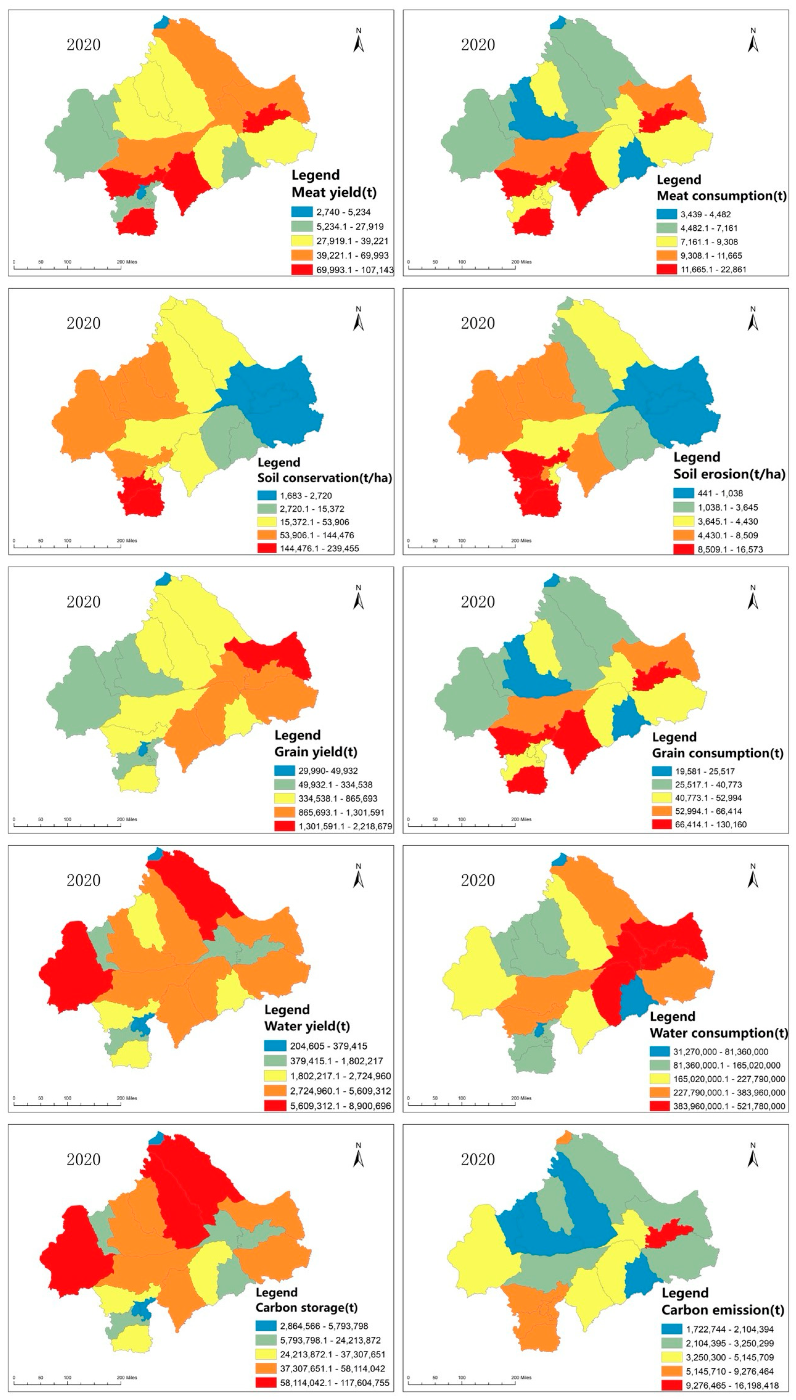
2.4. Carbon Storage and Carbon Emission

The carbon module in the InVEST model (3.14.0) was adopted to evaluate and calculate the supply of carbon storage [27], including above-ground biochar, below-ground biochar, soil organic carbon, and dead organic matter. The supply calculation formula is as follows:

$$C_{ct}=C_{above}+C_{below}+C_{soil}+C_{dead}$$

(1)

where $C_{ct}$ refers to the total carbon storage within the study area of each county, and $C_{above}$, $C_{below}$, $C_{soil}$, and $C_{dead}$ represent the above-ground biochar, below-ground biochar, soil organic carbon, and dead organic matter in the county, respectively.

Demand: Carbon emission is selected as a demand index for carbon storage [28]. The demand calculation formula is as follows:

$$C_{PC}=\frac{{\sum }_{i=1}^n{C}_i\times {EF}_i}{{POP}_y}$$

(2)

$$C_{cd}=C_{PC}\times C_{POP}$$

(3)

where $C_{cd}$ is the carbon emission of the study area in each county (tons), $C_{PC}$ is the per capita carbon emission (tons), $C_{POP}$ is the total population of each county, $C_i$ is the $i$-th type of energy consumption, $n$ is the type of energy consumption, ${EF}_i$ is the carbon emission factor of the $i$-th type of energy, and ${POP}_y$ is the total population in year $y$.

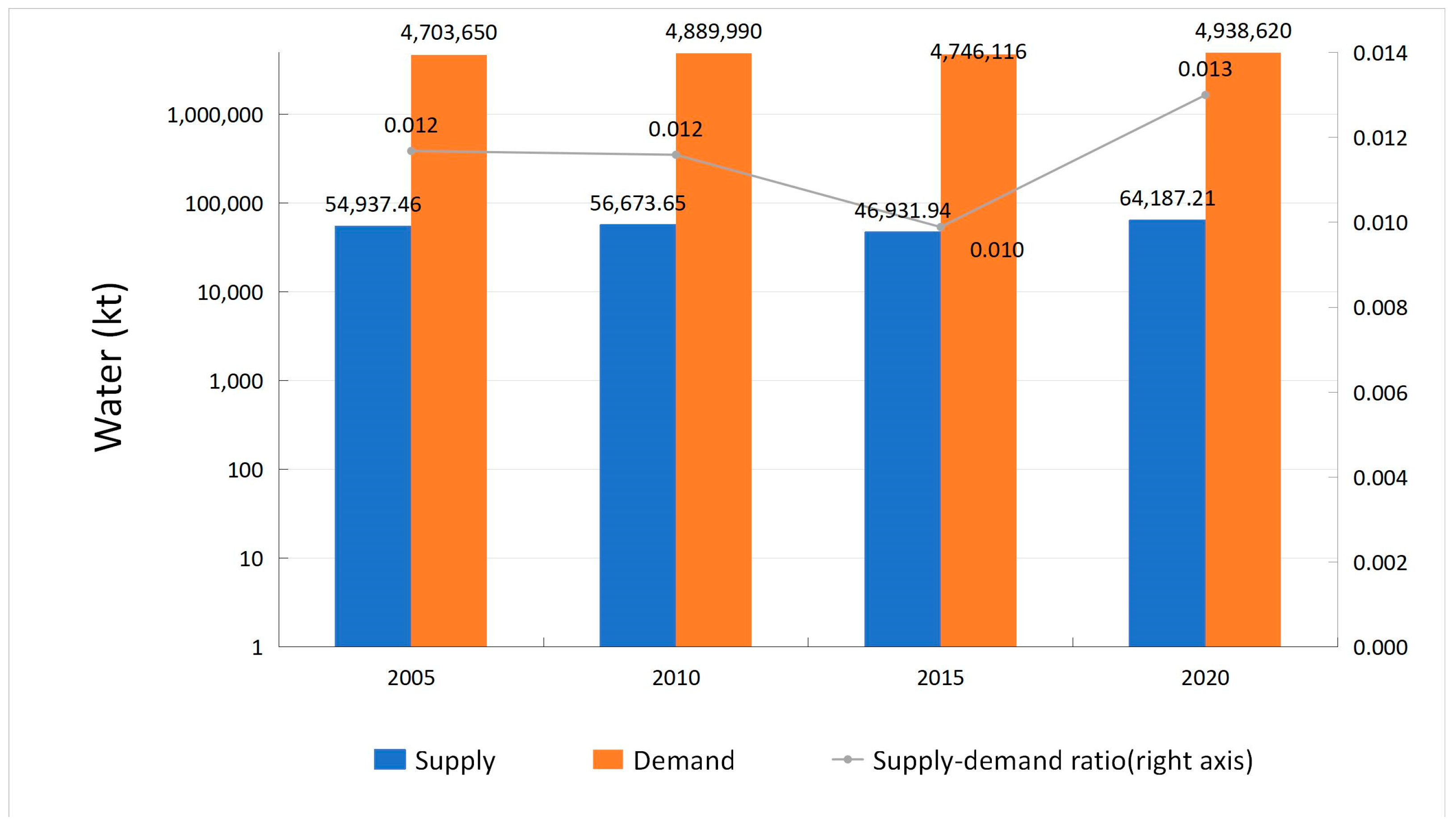
2.5. Water Yield and Water Use

Since most of the West Liao River Basin is in arid and semi-arid areas where evaporation exceeds precipitation, water resources are essential for sustainable development in the region. This study used the water yield module in the InVEST model (3.14.0) to calculate water production as supply [29]. The supply calculation formula is as follows:

$$W_{ct}=\left(1-\frac{{AET}_{cT}}{P_{ra}}\right)\times P_{ra}$$

(4)

where $W_{ct}$ is the annual water yield of the study area in each county (mm), ${AET}_{cT}$ is the actual yearly evaporation of the study area in each county (mm), and $P_{ra}$ is the total annual precipitation in the West Liao River Basin (mm).

Demand: The sum of domestic water, agricultural water, and industrial water at the county level in Chifeng City Water Resources Bulletin [30] and Tongliao City Water Resources Bulletin [31] is used to represent water demand. The demand calculation formula is as follows:

$$W_t=DW+IW+AW$$

(5)

where $W_t$ indicates the total water usage for each county (in tons), $DW$ represents the domestic water consumption (tons), $IW$ represents the industrial water consumption (tons), and $AW$ represents the agricultural water consumption (tons).

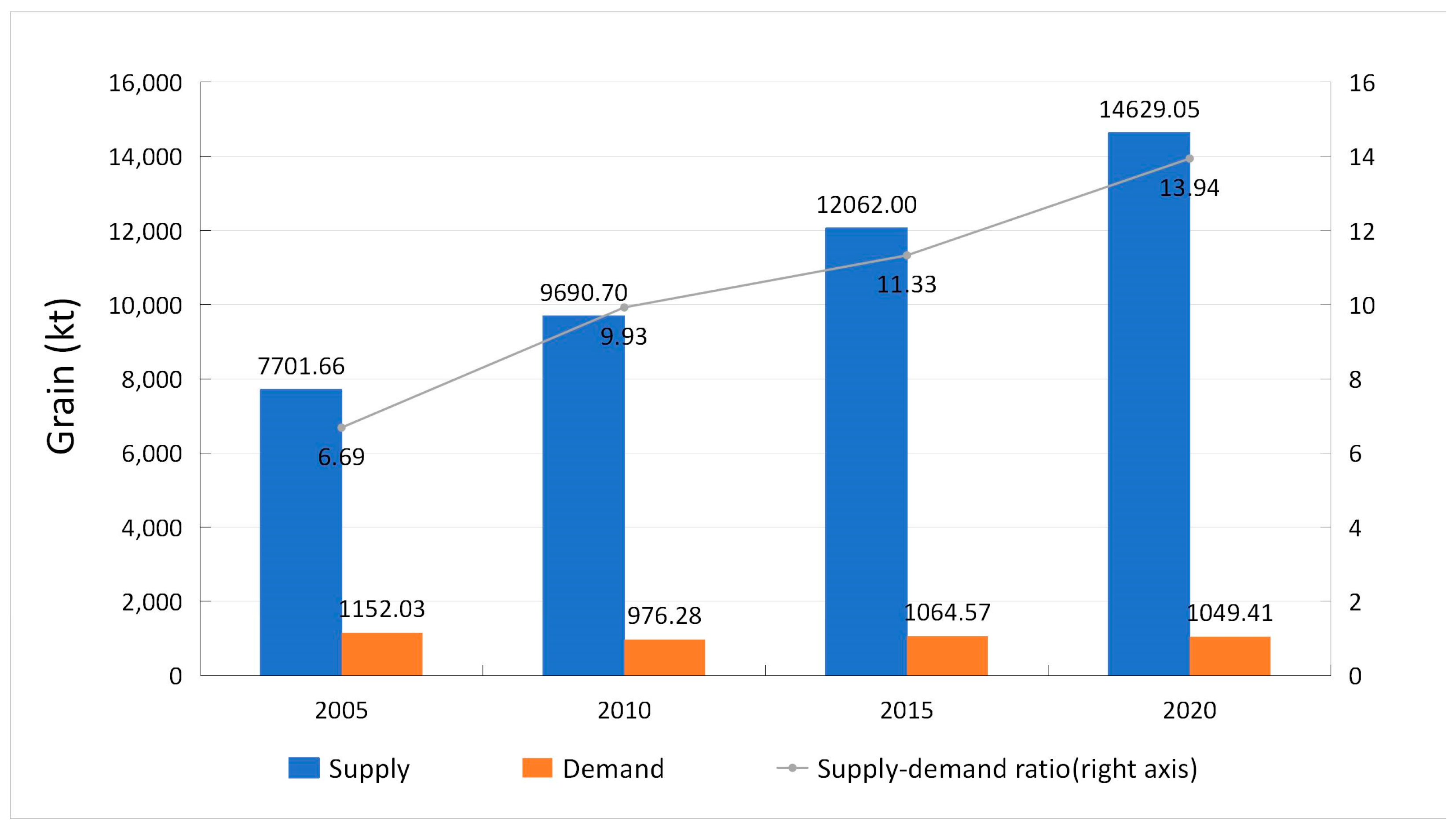
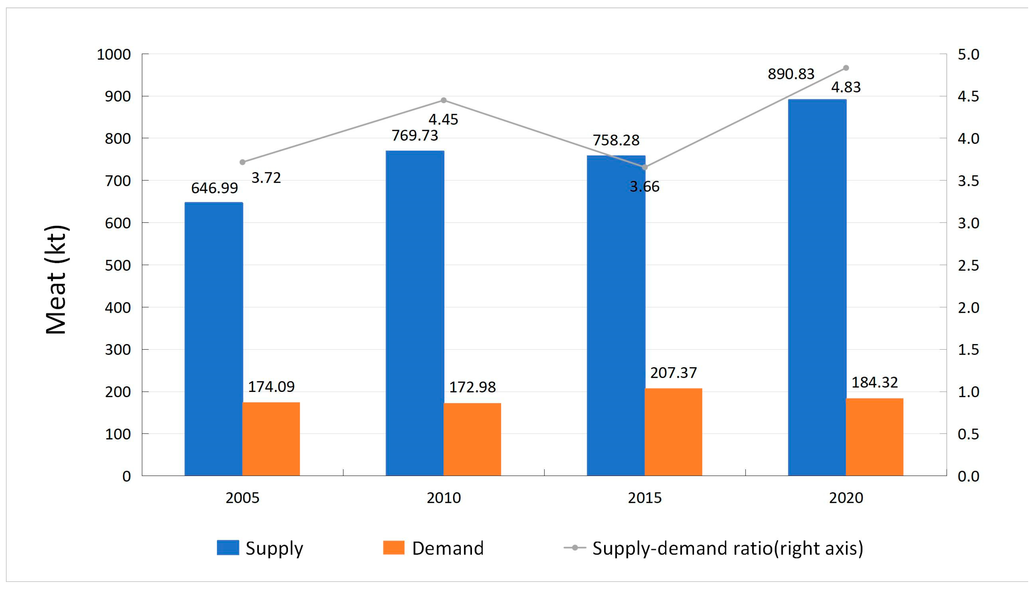
2.6. Meat and Grain Production

Food and meat are living necessities for residents, and they are mainly offered by the ES system. Given the strong linear correlation between crop yield and NDVI [32], this paper calculated grain or meat production based on the ratio of the NDVI of the grid in the study area to the NDVI of grassland or agricultural land [33], determined the grain supply capacity of each grid, and estimated the grain supply in the study area. Grain and meat production includes wheat, corn, millet, soybeans, pork, beef, and mutton. The supply calculation formula is as follows:

$$F_{tx}=F_{sum}\times \frac{{NDVI}_x}{{NDVI}_{SUM}}$$

(6)

where $F_{tx}$ represents the total grain or meat production (tons) of the study area in each county, $F_{sum}$ represents the total grain or meat production of the West Liao River Basin, ${NDVI}_x$ represents the $NDVI$ of grid $x$, and ${NDVI}_{SUM}$ represents the total $NDVI$ of grassland or agricultural land in the study area.

Demand: In this study, the demand for grain or meat was calculated by multiplying per capita consumption with the population of each study area [34]. The demand calculation formula is as follows.

$$D_{ra}=D_{PC}\times D_{pop}$$

(7)

where $D_{ra}$ is the demand for grain or meat in the study area of each county (tons), $D_{PC}$ is the per capita consumption of grain or meat in Inner Mongolia (tons), and $D_{pop}$ is the total population of each study area.

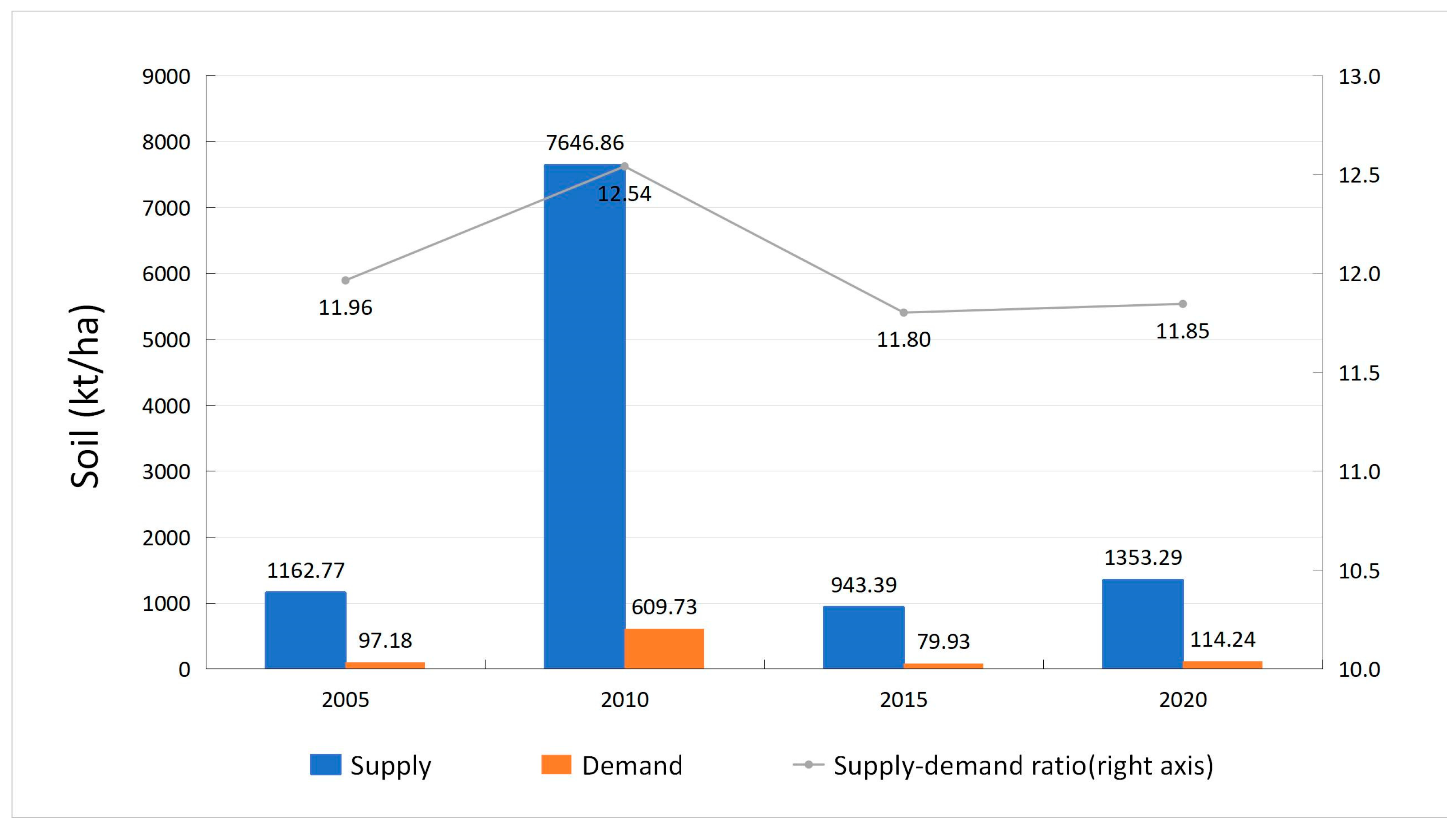
2.7. Soil Conservation

The SDR module in the InVEST model (3.14.0) was adopted to evaluate and calculate the amount of soil conservation [35]. The supply calculation formula is as follows:

$$S_{ct}={SPE}_{ct}-{SAE}_{ct}$$

(8)

where $S_{ct}$ is each county’s soil conservation amount, ${SPE}_{ct}$ is each county’s potential soil erosion, and ${SAE}_{ct}$ is the actual soil erosion.

Demand refers to the amount of soil erosion that humans expect to be controlled through human intervention. The demand calculation formula is as follows:

$${SAE}_{ct}=P\times C\times K\times LS\times R$$

(9)

where $P$ is the factor of soil conservation, $C$ is the factor of vegetation cover, $K$ is the factor of soil erosion, $R$ is the factor of rainfall erosion, and $LS$ is the factor of slope.

2.8. ES Supply–Demand Ratio

The ES supply–demand ratio is an essential index for intuitively understanding the balance between supply and demand. In contrast, the spatiotemporal variation trend of the supply–demand ratio is significant for achieving sustainable regional development [36]. The supply calculation formula is as follows:

$$E_r=\frac{E_s}{E_d}$$

(10)

where $E_r$ is the ES supply–demand ratio of the ES index, $E_s$ is the index’s supply, and $E_d$ is the index’s demand.

2.9. Construction of Coupling Coordination Model

According to the actual situation of the West Liao River Basin, we selected water yield, carbon storage, water quality purification, grain and meat production as supply and demand indexes to construct an evaluation index system, adopted the entropy weight method to calculate the weight of each index, and used the coupling coordination model for calculation. The calculation method is as follows:

2.9.1. Dimensionless Index

$$X_{cs}=\frac{X_{sd}-X_{min}}{X_{max}-X_{min}}$$

(11)

In the formula, $X_{cs}$ is the standardized value of index S in County C, $X_{sd}$ is the supply or demand value, and $X_{max}$ is the maximum value of supply or demand. At the same time, $X_{min}$ is the minimum value of supply or demand.

2.9.2. Use the Entropy Weight Method to Calculate the Weight of Each Index

The calculation method is as follows:

$${PR}_{cs}=\frac{0.0001+X_{CS}}{{\sum }_{c=1}^n{\sum }_{s=1}^n\left(0.001+X_{cs}\right)}$$

(12)

$$E_s=-\frac{1}{\mathit{ln}\left(n\right)}\sum _{c=1}^n{PR}_{cs}\times \mathit{ln}\left({PR}_{cs}\right)$$

(13)

$$G_s=1-E_s$$

(14)

$$W_s=\frac{G_s}{{\sum }_{s=1}^n{G}_s}$$

(15)

where ${PR}_{cs}$ is the proportion of index S in County $C$, $E_s$ is the S entropy index, $G_s$ is the S difference coefficient, and $W_s$ is the weight of $S$ [37].

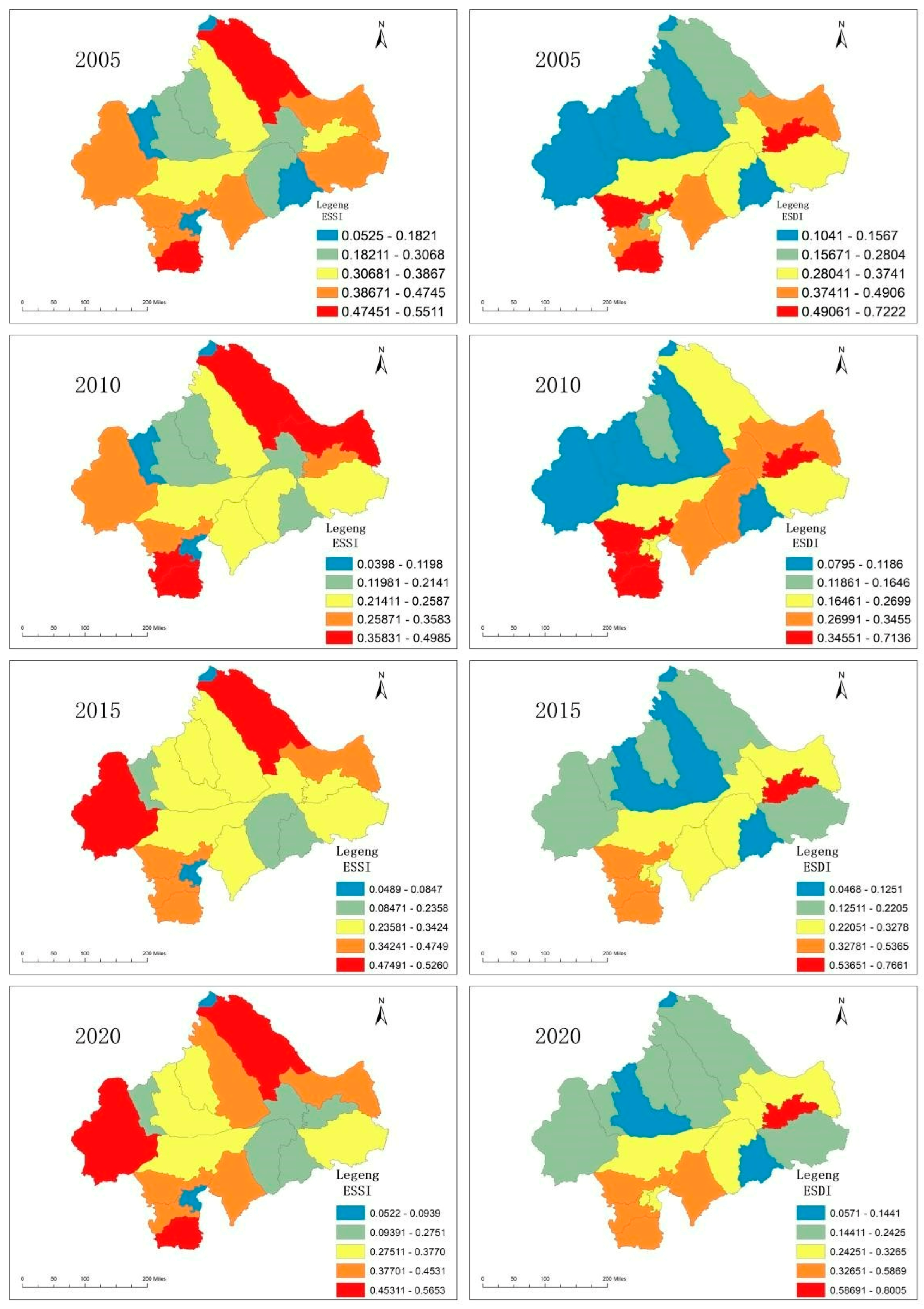
2.9.3. Calculate the ES Supply Index (ESSI) and ES Demand Index (ESDI)

The calculation method is as follows:

$$ESSI or ESDI=\sum _{s=1}^n{W}_s\times {PR}_{cs}$$

(16)

where $ESSI$ and $ESDI$ are the ES supply-synthesized coefficient and demand-synthesized coefficient, respectively. The $ESSI$ and $ESDI$ reflect the changes in the ES supply–demand in the West Liao River Basin from 2005 to 2020 [38].

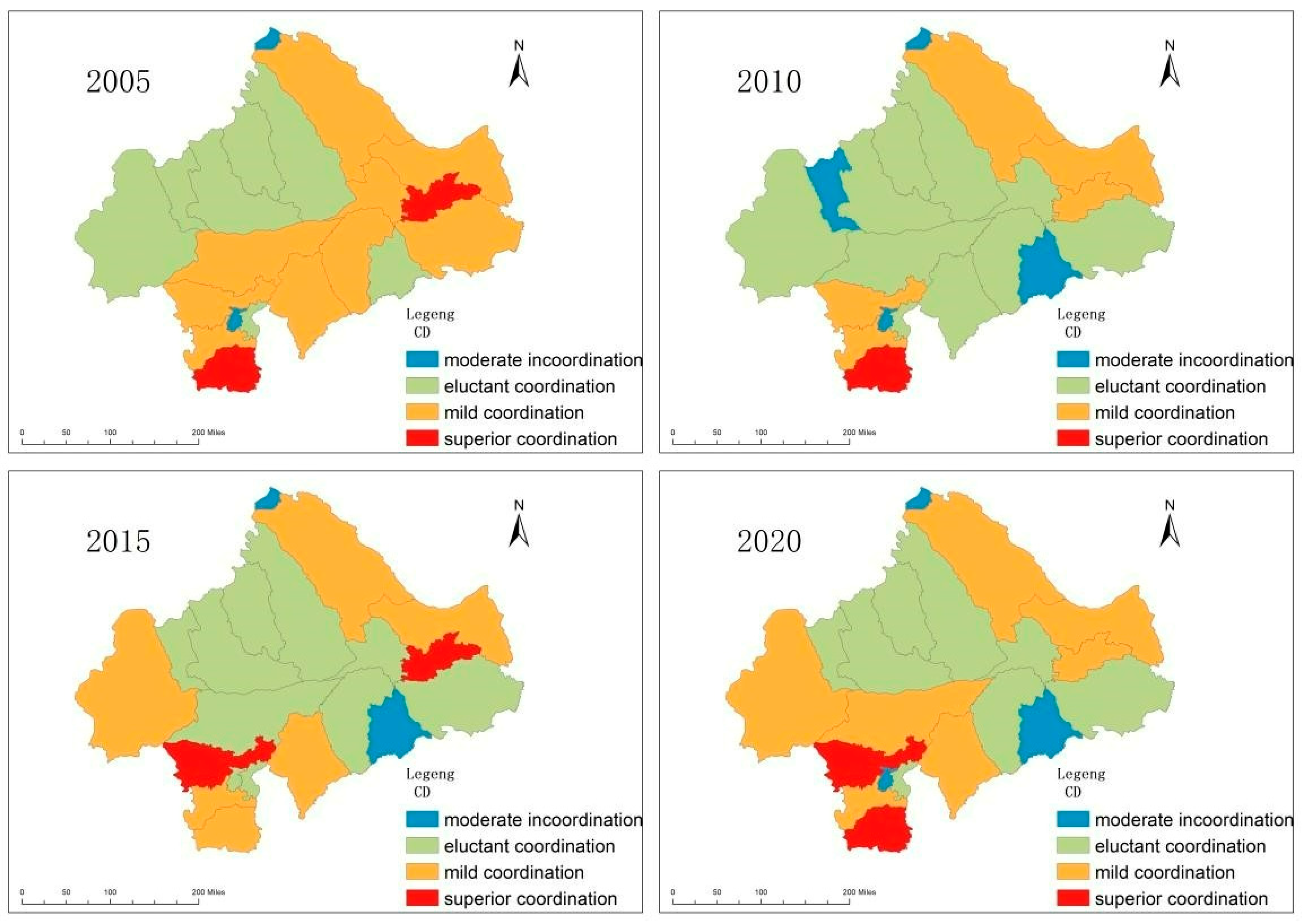
2.9.4. Construction of Coupling Coordination Degree Model

Based on the ESSI and ESDI, the coupling coordination degree model is adopted to explore the ES supply–demand relationship. The calculation method is as follows:

$$C=2{\left[\frac{(ESSI\times ESDI)}{\left(ESSI+ESDI\right)2}\right]}^{1/2}$$

(17)

$$T=\alpha \times ESSI+\beta \times ESDI$$

(18)

$$CD=\sqrt{C\times T}$$

(19)

where $C$ is the coupling degree between supply and demand, $T$ is the comprehensive development index of the ES supply and demand, $\alpha$ and $\beta$ are the weights of $ESSI$ and $ESDI$, respectively, and the ES supply and demand are equally important. Therefore, $\alpha$ = $\beta$ = 0.5. The $CD$ is the coupling coordination degree at the county level. According to previous research, $CD$ can be divided into five stages, as shown in

Table 1. Classification of coupling coordination degree.

Coupling Value	Coupling State
0 ≤ CD ≤ 0.20	extreme incoordination
0.20 ≤ CD ≤ 0.35	moderate incoordination
0.35 ≤ CD ≤ 0.55	basic coordination
0.55 ≤ CD ≤ 0.70	mild coordination
0.70 ≤ CD ≤ 1	superior coordination

[39].

2.9.5. Construction of Supply and Demand Matching Model

To further clarify the relationship between ESSI and ESDI, a supply and demand matching model (MD) is built. When $MD$ > 1, the supply exceeds the demand. When $MD$ < 1, the supply fails to meet the demand. The calculation method is as follows:

$$MD=\frac{ESSI}{ESDI}$$

(20)

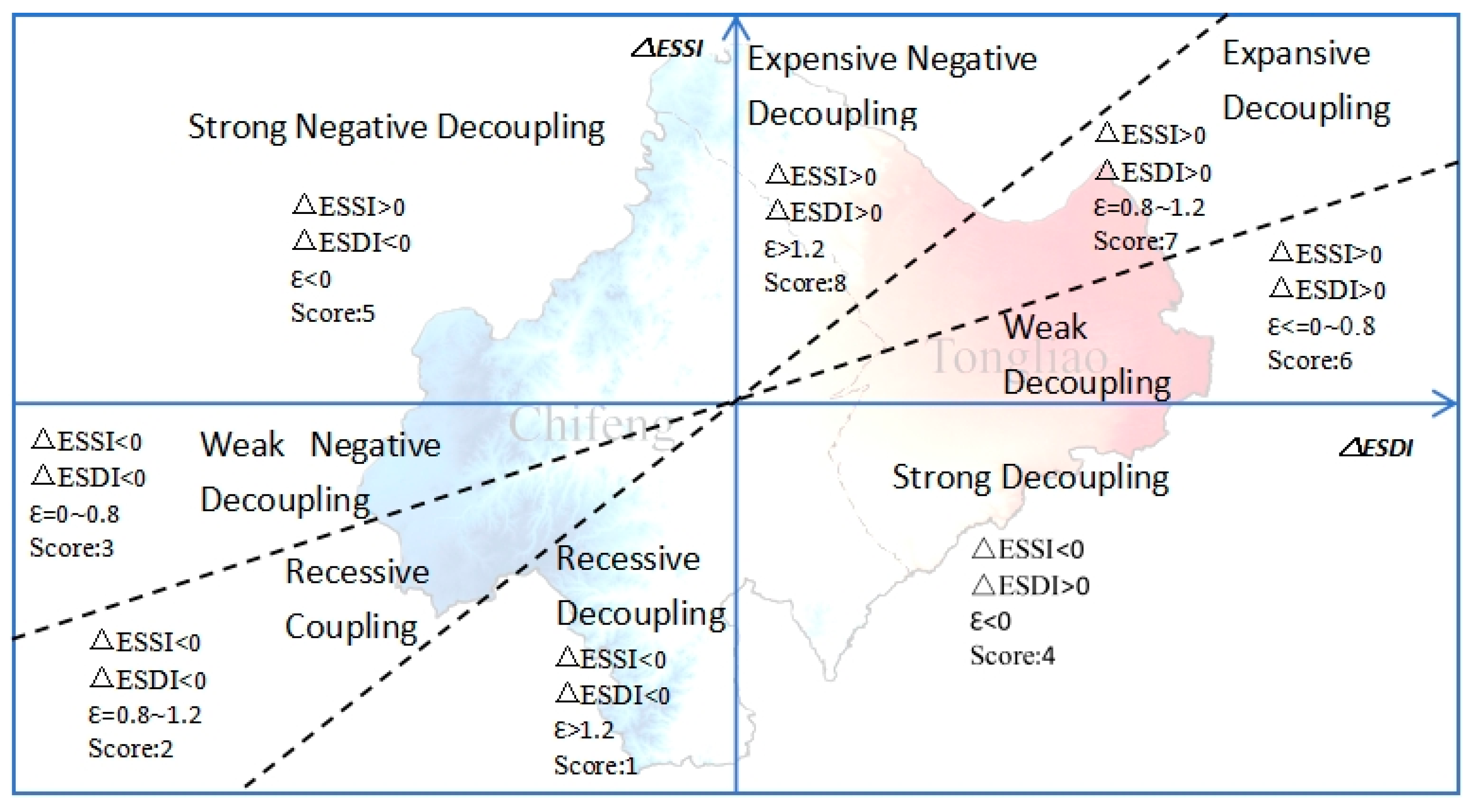
2.9.6. Decoupling Model

To gain a deeper understanding of the dynamic relationship and changes between the ES supply and demand at the county level, this paper assigned the ratio of the change rate of $ESSI$ (ΔS) to that of $ESDI$ (ΔD) to a decoupling model to calculate the decoupling index, thus evaluating their inter-relationships. The decoupling calculation method is as follows:

$${\epsilon }_t=\frac{({ESSI}_t-{ESSI}_{t-1})/{ESSI}_{t-1}}{({ESDI}_t-{ESDI}_{t-1})/{ESDI}_{t-1}}$$

(21)

where ${ESSI}_t$ and ${ESSI}_{t-1}$ are the ES supply indexes in year $t$ and year $t-1$, respectively; ${ESDI}_t$ and ${ESDI}_{t-1}$ represent the ES demand indexes in year $t$ and year $t-1$, and εt is the decoupling index in year $t$. In the scoring system, a score of 8 represents the most ideal decoupling state, while 1 represents the least ideal decoupling state (Figure 2). Based on the decoupling index, the corresponding score is assigned according to previous studies to reflect the quality of the relationship between ES supply and demand [40].

2.10. Geographically and Temporally Weighted Regression (GTWR)

The GTWR model is an extension of the traditional geographically weighted regression (GWR) model, retaining the GWR’s ability to analyze the nonstationary relationships between variables in the spatial dimension. However, since there is also heterogeneity in the temporal dimension of ecosystem services, this model can explore the impact of explanatory variables on dependent variables across both time and space [41,42]. This study employed eight indicators (cropland area, forest area, grassland area, unused land area, GDP, population, NDVI, and water yield) as variables to analyze their spatiotemporal heterogeneity and impact on the coupling coordination degree in the West Liao River Basin. The selected variables directly or indirectly drive or are correlated with the ES. Normalization with z-score allows the dimensions between drivers to be kept at the same level. The drivers included annual precipitation, normalized vegetation difference index, population, GDP, cropland area, forest area, grassland area, water area, and unused land area. Finally, stepwise regression analysis was used to select significant variables and eliminate multicollinearity between variables, and a 5% significance level was used to select significant variables. The calculation method is as follows:

$$y_{in}={\beta }_0\left(m_i{n}_i\right)+\sum _{i=1}^k {\beta }_j \left(m_i{n}_i\right)x_{in}+{\rho }_{in}$$

(22)

where $y_{in}$ represents the dependent variable of the $i$-th sample point in the study area during period $n$, ${\beta }_j \left(m_i{n}_i\right)$ is the spatial geographic location coordinates of the $i$-th sample point in the study area, $x_{in}$ represents the independent variable of the $i$-th sample point in the study area during period n, and ${\rho }_{in}$ represents the random error term of the study area.

3. Results

3.1. Characteristics of Spatial and Temporal Variations in Supply, Demand, and Supply–Demand Ratios

Based on the InVEST model, Arcgis and statistical yearbook data, ecosystem services such as carbon storage, water production, grain production, meat production, and soil and water conservation in the West Liao River Basin were quantitatively analyzed in 2005, 2010, 2015, and 2020. The spatiotemporal quantitative mapping of supply, demand, and supply–demand ratios was conducted (Figure 3, Figure 4, Figure 5, Figure 6, Figure 7 and Figure 8), and quantitative maps were plotted for the year 2020 as an example.

On the time scale, carbon stocks in most areas showed a fluctuating decreasing trend from 2005 to 2020, but the percentage of decrease is small, and the percentage of decrease in carbon stocks in the Red Mountain area is larger at 5.63%. Carbon emissions all increased in the study area. Hongshan District, Horqin District, and Songshan District, as major industrial and economic centers, have significantly higher carbon emissions than other areas. The average growth ratio of carbon emission in the watershed was 135.93%.

Water production in the West Liao River Basin decreased by more than 16% from 2005 to 2015 but increased by 27% from 2015 to 2020, with a general upward trend. Bahrain Right Banner had the highest water yield and the fastest growth rate of 81%, while water yield in Linxi County decreased by 54%. Water consumption in the study area showed an upward trend, with Yuanbaoshan District showing a significant increase in water consumption growing to 44.55%. Other areas showed less fluctuation.

From 2005 to 2020, grain production in the study area showed a fluctuating increasing trend with an average growth rate of 7.47%. Yuanbaoshan District had the fastest growth rate of 80.85%. Production in Hongshan District and Huolinguole City was significantly lower than most other areas. Due to the decrease in population from 2005 to 2020, most of the areas showed a decreasing trend in food consumption, except for a few areas that showed a slight increase in 2020 compared to 2005.

Meat production exhibited an upward trend, with an average growth rate of 9.24%, mainly concentrated in the central and eastern parts of the basin, such as Horqin Left Middle Banner, from 2005 to 2020. Meat consumption increased in most of the districts and demonstrated a decreasing trend after consumption peaked in 2015. The areas with higher demand for soil conservation were Ningcheng County, Songshan District, and Harqin Banner, while the lower demand was in the central and eastern parts of Tongliao City.

According to the supply–demand ratio, the supply–demand ratios of grain production and soil and water conservation were found to be always greater than 1, the supply–demand ratios of carbon resources in seven counties were less than 1, and the supply–demand ratios of other regions were greater than 1. The supply–demand ratios of carbon resources and soil and water conservation stabilized since 2010, while the supply–demand ratios of grain and meat increased year by year. The supply–demand ratios of water resources showed an increasing and then decreasing trend.

The West Liao River Basin is a typical semi-arid agricultural and pastoral zone in northern China, characterized by animal husbandry and agricultural development. The study area plays a crucial role in providing ecological services, with the supply of all ecosystem services in the region—except for water resources—substantially exceeding demand. This is consistent with results from neighboring areas studied by Zhang et al. [43]. This suggests that the ecosystem services offered by the West Liao River Basin significantly support the development of the area.

3.2. Spatial and Temporal Dynamics of ESSI and ESDI

The significant changes in the ESSI in the West Liaohe River Basin from 2005 to 2020 are shown in Figure 9. The ESSI showed a downward trend averaging 6.9% from 2005 to 2010. The ESSI increased slowly from 2015 to 2020 in a “U”-shaped trend. From 2005 to 2020, most of the regions show an upward trend in ESSI, indicating an increase in overall demand. The northern and central parts of the study area have lower ESSI indexes due to underdeveloped agriculture and industry, among other reasons. Jarud Banner and Horqin Left Middle Banner in the northeast, as well as Ningcheng County, Songshan District, and Harqin Banner in the southwest, have higher ESSI indexes due to superior original ecological resources. Meanwhile, the ESDI index in the southern region was significantly larger than that in the northern region.

ES supply is based on the carrying capacity of the ecosystem and the degree of human utilization of the ecological service system. Supply is divided into potential supply and actual supply, where potential supply is the capacity of the ecological service system that can provide services sustainably in the long term, and actual supply is the ecological process consumed or utilized by human beings, and ES demand is the actual supply. The relationship between supply and demand is interdependent and interactive; when the supply is greater than the demand can ensure normal social relations, on the contrary, it indicates that human utilization of natural resources in the region has exceeded the carrying capacity of the ecosystems in the region, which often causes problems such as ecological degradation and damage to human well-being. This situation can be assessed at multiple levels in order to understand the trend of change between the supply of and demand for ES.

3.3. Spatiotemporal Influence of CD and MD

The CD of the West Liao River Basin in 2005–2020 is shown in Figure 10. The CD values are higher in the northeastern and southwestern areas, while they are lower in the central region. Although the CD value decreased by 11% from 2005 to 2010, the CD value showed an increasing trend from 2010 to 2020, with an increase of more than 10%. The overall CD reached 0.54, close to mild harmonization, and the overall trend is “U” shaped. It indicated that ES sustainability improved in the study area from 2005 to 2020. Both showed spatial heterogeneity. The results showed that the overall trend in Horqin was decreasing, changing from excellent coordination (0.72) to moderate disharmony (0.68). The CD of Songshan District increased year by year, reaching (0.71) excellent coordination. The change in CD value in other areas showed a decreasing and then increasing trend, indicating that some achievements were made in resource utilization and environmental protection, but further optimization is still needed.

Figure 11 shows the trend in MD value in the study area from 2005 to 2020, with overall values elevated in the north and reduced in the south, steadily increasing during 2005–2015 and stabilizing in 2015–2020, with the overall value being greater than 1, indicating that the overall supply is greater than demand. The MD index of Horqin District, Xilingol League, and Hongshan District shows a decreasing trend and is always less than 1, indicating an imbalance between supply and demand, with supply less than demand. Yuanbaoshan District, Naiman Banner, and Songshan District show an increasing trend although the MD index is less than 1. The other areas have a small increase or decrease but generally remain greater than 1.

The sustainability indicator quantifies the degree of sustainability of the ES and reflects the degree of deviation of the ESCI and ESDI relative to the two mean values based on the concept of deviation. The smaller the deviation, the higher the CD and ES sustainability values. To analyze the interdependence between ES supply and demand subsystems, a natural resource system model based on the coupled coordination framework was developed. MD solves the practical problem of the ES carrying degree, which is affected by both the ecosystem supply capacity and human consumption behavior.

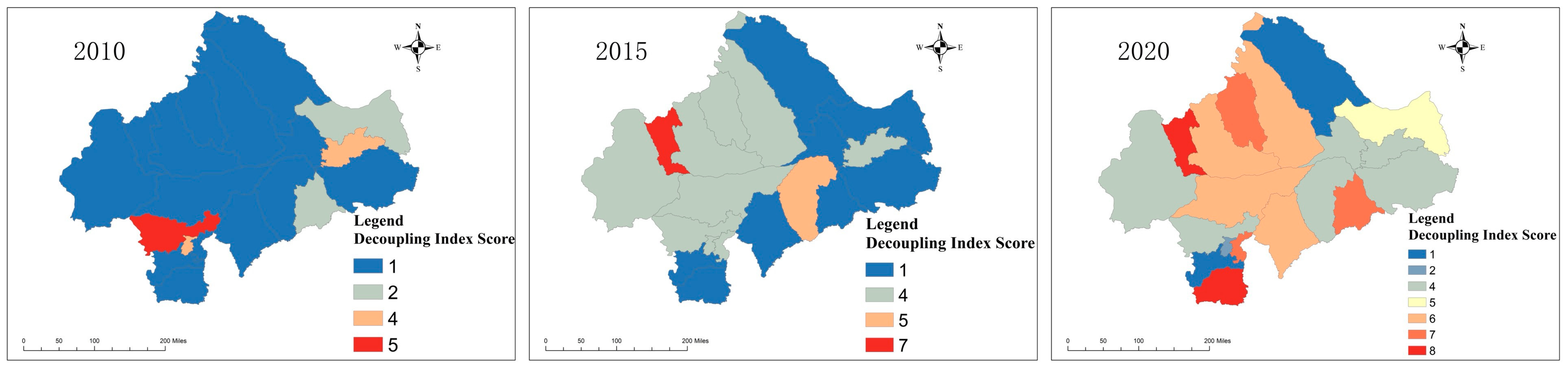
3.4. Spatial and Temporal Variation in Decoupling Indices

After examining the temporal pattern of coupling coordination degree, the decoupling index model was constructed with the aim of exploring the dynamic evolution of the coupling coordination degree between ecosystem service supply and demand. The decoupling index score of the West Liao River Basin showed a large upward fluctuation during 2005–2020, as shown in Figure 12, and the coupling coordination degree declined in most areas during 2005–2010, and the decoupling index scores of the 17 counties with a declining trend were mostly 1, which indicated that there was a double decline in supply and demand. Ten counties had a decoupling index score of 4 during 2010–2015, which indicated that supply declined but demand increased. During the period of 2010–2015, 10 counties had a decoupling index score of 4, indicating a decline in supply but a rise in demand, at which time the supply and demand for ecosystem services were in a state of mutual antagonism; 8 counties had a decoupling index score of 1; and only 2 counties had a score of more than 5. During the period of 2015–2020, 10 counties had a decoupling index score of more than 6, indicating that there was a both rise in the supply and demand for these counties. Horqin District, the central area of Tongliao City, had a decoupling index of 4 for 15 years, indicating that its supply decreased while demand increased. The decoupling index of Hongshan District, the central urban area of Chifeng City, showed a downward trend in the past 15 years, indicating that its supply–demand relationship shifted from mutual antagonism in 2015 to a double decline. Songshan District was developed into a new main urban area to meet the demand for urban development, resulting in a shift from increased supply and decreased demand to decreased supply and increased demand. Most of the county with low scores double-declined in 2010 into mutual antagonism in 2015 before finally increasing to high scores of the year 2020, demonstrating a strong decoupling state. It showed that the coupled and coordinated relationship between the supply and demand of ecosystem services in the study area was further improved.

3.5. GWTR

In this study, stepwise regression was utilized to identify significant variables, thereby circumventing multicollinearity between variables (p < 0.05, variance inflation factor < 7.5) (

Table 2. Results of the stepwise regression.

Variables	p Value	Variance Inflation Factor
Population	<0.01	4.28
GDP	0.03	6.83
NDVI	<0.01	5.78
Precipitation	<0.0001	4.47
Cropland	0.02	6.42
Forest land	<0.001	5.61
Grasslands	0.02	5.92
Unused land	<0.0001	3.43

). The range of values is −1~1. If the value is between 0 and 1, it means that the variables are generally positively correlated with each other; if the value is less than 0, it means that the spatial variables are generally negatively correlated with each other. Figure 13, Figure 14, Figure 15, Figure 16, Figure 17, Figure 18, Figure 19 and Figure 20 show the spatial and temporal heterogeneity of the factors influencing the degree of coupling coordination.

(1)

population declines in Horqin District, Horqin Left Rear Banner, Hure Banner, Bairin Left Banner, Kailu County, Naiman Banner, Horqin Left Middle Banner, and Aohan Banner exerted a positive impact on the coupling coordination degree. In contrast, the population change in other regions negatively influenced the degree of coupling coordination. The average impact coefficients were 0.0005, 0.0007, 0.0013, and 0.0029, respectively, showing a rising trend, which demonstrates that the impact of population on the relationship between supply and demand for ES is gradually increasing.

(2)

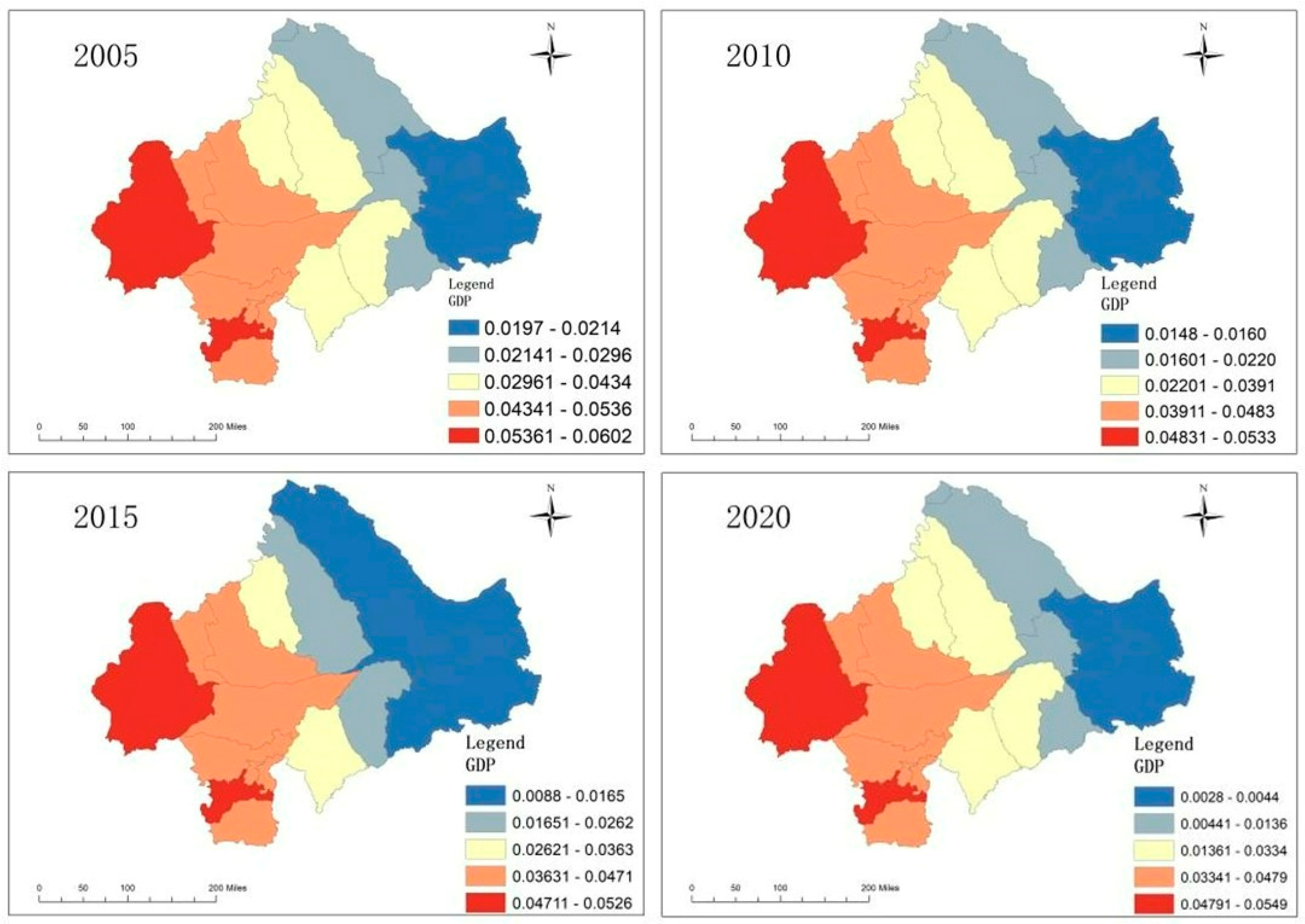
The influence coefficients of GDP per capita in all counties were all greater than 0, indicating that GDP per capita has a positive influence on the coupling coordination degree from 2005 to 2020. The average influence coefficients were 0.0399, 0.0346, 0.0314, and 0.0292, respectively, showing a decreasing trend, indicating that the influence of GDP on ES supply and demand relationship is gradually decreasing.

(3)

From 2005 to 2010, the NDVI coefficients of the seven counties were all negative, indicating that they had a negative impact on the coupling coordination degree. The NDVI coefficients were all greater than 0, indicating that NDVI had a positive influence on the coupling coordination degree. The average influence coefficients were 0.0099, 0.0188, 0.0277, and 0.0331 respectively, showing an increasing trend, which indicates that the influence of NDVI on ES supply and demand relationship is gradually increasing.

(4)

From 2005 to 2020, the coefficient of annual rainfall, one of the influencing factors, was greater than 0, indicating that rainfall has a positive influence on the coupling coordination degree. The average influence coefficients were 0.0625, 0.0634, 0.0652, and 0.0671, respectively, and the positive influence of precipitation on the degree of coupling coordination gradually increases, indicating that the influence of precipitation on the relationship between supply and demand of ES gradually increases.

(5)

During the period from 2005 to 2020, the coefficient value of the influence factor of cultivated land area was greater than 0, indicating that cultivated land area has a positive influence on the coupling coordination degree. The average influence coefficients of 0.0964, 0.0988, 0.1003, and 0.1006 proved that the positive influence of cultivated land area on the degree of coupling coordination shows a gradual upward trend.

(6)

From 2005 to 2020, the coefficient of forest, one of the influence factors, was greater than 0, indicating its positive influence on the degree of coupling coordination. The average influence coefficients were 0.509, 0.5038, 0.4941, and 0.4859, respectively, indicating that the positive influence of forests on the degree of coupling coordination weakened during this period.

(7)

From 2005 to 2020, the coefficients of the grass influence factor were all greater than 0, indicating that grass has a positive influence on the degree of coupling coordination. The average influence factor coefficients were 0.3531, 0.3467, 0.3402, and 0.3368 respectively, indicating that the positive influence of grassland on the coupling coordination degree weakened during this period.

(8)

From 2005 to 2020, the coefficient of unused land, which is one of the influencing factors, was less than 0, indicating its negative influence on the coupling coordination degree. The average influence coefficients were −0.1820, −0.1808, −0.1661, and −0.1494, respectively, indicating that the negative influence of unutilized land on the degree of coordination of the coupling weakened during this period.

According to the results of GTWR, the population coefficient was high in the eastern region and low in the western region; the GDP coefficient was high in the Hexigten Banner and Harqin Banner and low in the eastern region; the precipitation coefficient was high in the southern flags and counties of Chifeng and low in the northeastern part; the NDVI coefficient was high in the eastern region and low in the western region; the grassland coefficient was high in the southern region and low in the northern region; the forest coefficient was higher in the western region and lower in the eastern region, while the unutilized land coefficient was higher in the east and lower in the central and western regions. Overall, there were clear spatial variations in the coefficients at the county level.

4. Discussion

4.1. Understanding the Spatial and Temporal Dynamics of ES Supply and Demand Relationships

This paper presented a detailed analysis of the spatial and temporal variations in the supply and demand of five ecosystem services (ES) in the West Liao River Basin from 2005 to 2020. It introduced the decoupling model and geographically weighted regression (GTWR) to examine the associated constraints. Our findings revealed that the supply of most ecosystem services exhibited a fluctuating upward trend, except for soil retention, which showed a fluctuating downward trajectory. As a vital grain production base in northern China and a key ecological security zone, the West Liao River Basin primarily focuses on grain production and maintaining ecological and environmental stability, aligning with the conclusions of this study.

The spatial and temporal dynamics of ES supply and demand were influenced by policy implementation and changes in vegetation coverage within the study area. The decline in the Ecosystem Services Supply Index (ESSI) between 2005 and 2010 was primarily due to the conversion of farmland, forests, and grasslands into urban and industrial areas. However, a range of policies—such as the construction of high-standard farmland, adoption of modern agricultural technologies, and the “Three Rural Development” initiative—enabled an increase in ESSI from 2010 to 2020. These measures improved the previously degraded ecosystem, maintaining the West Liao River Basin’s ES supply at a high level. Significant regional disparities in ESSI levels were observed, with eastern and southern counties outperforming central ones due to their abundant natural resources, consistent with the findings of Wei et al. [44].

In 2010–2020, the level of ESSI in the counties of the West Liao River Basin continued to increase. According to the entropy weighting results, soil retention accounted for the largest share (0.29) of this change, but this value decreased in 2010, indicating a downward trend in its weighting index. Meanwhile, the share of water production increased year by year, reaching 0.19, which has a significant contribution to the development of ESSI. The counties ESDI showed a decreasing trend, and according to the entropy weighting results carbon emissions accounted for the largest share (0.28). Overall, the relationship between the supply and demand of ES was synergistic with the population density, and the demand of the more populated counties was significantly higher than the other areas. These results are consistent with the results of Wen et al. [45].

4.2. Temporal Dynamics of CD and Decoupling Index Scores

The coupled coordination degree (CD) of ecosystem services (ES) reflects a region’s carrying capacity and potential for sustainable development. To analyze this, a resource supply-and-demand relationship model was constructed using the coupled coordination framework. This study incorporated the measures of mismatch degree (MD) and CD to investigate the spatial and temporal patterns of the ES supply–demand ratio and their coordination dynamics. Overall, CD at the watershed scale exhibited a decline followed by a recovery, while MD consistently remained greater than 1.

Despite the West Liao River Basin’s resource abundance, rapid economic growth in China and higher population density in this region compared to the rest of Inner Mongolia have led to heightened demand for ES. In some areas, the supply wad insufficient to meet this demand, causing the overconsumption of natural resources in certain counties. This imbalance, coupled with increasing natural resource constraints, hampered the sustainable development of affected areas. As ES supply diminishes and demand growth rates slow down, many counties struggle to achieve sustainable progress. To address these challenges, local governments must implement targeted policies to enhance ES supply and address mismatches in coordination, ultimately fostering sustainable development goals.

Based on this coupled spatial and temporal pattern of coordination degree, this paper established a decoupling index model to analyze the dynamic changes in the coordination degree of ecosystem service’s supply and demand relationship. The decoupling index score of the West Liao River Basin showed fluctuating changes from 2005 to 2020. The rapid expansion of urban construction land, serious shrinkage of grassland area, and degradation of farmland in the West Liao River Basin during 2005–2010 were serious threats to the sustainability of the ES, explaining why both the CD and the decoupling index scores showed a downward trend in 2010. In addition, it is important to note that the decoupling index score will stay at 5 (ΔESSI > 0, ΔESDI < 0) if we want the ES and CD to improve again in the future.

Based on the above results, and considering the significant strong coupling coordination between ES supply and demand, we found that the constraint of diminishing urbanization constrained the development of the ecosystem. In addition, we found that the spatial patterns of CD and ESSI were highly consistent. High CD usually occurred in areas with high ESSI. The reason for their high CD is that their rich natural resources have a high supply capacity. On the contrary, the deterioration of soil conditions and the increase in water evaporation due to the more rapid urbanization and arid climates in some areas constrain the development of ESSI, which, in turn, constrains the development of CD. This suggests that improvements in the natural environment can promote the development of ecosystem services. Although the West Liao River Basin achieved remarkable results in improving CD between 2005 and 2020, more efforts are needed to ensure the simultaneous improvement in ES supply and demand.

4.3. Spatial and Temporal Dynamics of Impact Factors

According to the ecological economics theory, economic development and the natural environment are closely inter-related, with each capable of either constraining or enhancing the other [46]. To better understand the spatial and temporal influences of key factors affecting the relationship between the supply and demand of ecosystem services (ESs) on the coupled coordination degree (CD) [47], this study employed the geographically and temporally weighted regression (GTWR) model. This approach identified the primary drivers of CD variations, offering a robust scientific foundation and practical guidance for ecological conservation decision making.

With a rainfall coefficient greater than 1, the West Liao River Basin experiences a dry climate. Rainfall not only enhances the natural environment but also strengthens the relationship between ecosystem service supply and demand. This conclusion is the same as that of Liu et al. [48]. The coefficient value of forest land is greater than 1 and remains stable, indicating that forest land has a large and stable influence on the relationship between ES supply and demand, and this phenomenon indicates the effectiveness of the policy of returning farmland to forest, which is consistent with the findings of [49,50]. The NDVI coefficient and GDP coefficient are both positive. Many studies proved that precipitation is conducive to improving CD; our results also confirmed this conclusion [48]. Although the values of the coefficients of cultivated land are all greater than 1, their impact indexes are decreasing, indicating that the positive impact of cultivated land on ES supply and demand is weakening. Excessive cultivation will not only lead to soil structure destruction and fertility decline but also increase the demand for irrigation and thus aggravate the over-exploitation of groundwater, leading to water shortage and water quality deterioration [51]. According to Wolfram et al. calculations, the global biomass production potential exceeds the expected future demand without the need to expand the area of arable land [52].

5. Conclusions and Policy Recommendations

5.1. Policy Recommendations

Between 2005 and 2020, forest area in the study area increased by more than 700,000 hectares, but grassland area decreased by more than 1.82 million hectares. In addition, the area of agricultural land rapidly expanded by 1.2 million hectares. In this case, the expansion of cropland area stimulated evaporation, leading to a continuous decline in the water supply/demand ratio in some areas. As a result of the significant expansion of farmland, the use of fertilizers increased, leading to an increase in groundwater pollution and a decline in the supply of agricultural soil retention. In conclusion, water scarcity and grassland degradation are major ecological problems in the West Liao River Basin. Returning farmland to forests can help to improve water resource production in arid areas. Therefore, the West Liao River Basin should further implement the strategies of “returning farmland to forests” and “integrated restoration of mountains, waters, forests, fields, lakes, grasslands and sands” and introduce corresponding water conservation policies to bridge the gap between the water supply and demand in the study area. From a county perspective, the supply in the northeast and southwest is significantly higher than in other regions, so it is recommended to continue maintaining a high level of supply to sustain ecological stability and food security in the West Liao River region. In the southern region, although the supply is higher, the demand is also greater and more sensitive to population changes, so it is necessary to further implement the construction of high-standard farmland to meet the needs of the local population.

5.2. Conclusions

Correct understanding of ES supply and demand is important for promoting regional ecological management and sustainable development. In this paper, the spatial and temporal patterns of supply, demand, supply–demand ratio, matching degree, and coordination degree of five ESs from 2005 to 2020 were analyzed at county and watershed levels with the West Liao River Basin as the object of study, and a decoupling index model was established on this basis to analyze the dynamic changes in the coupling coordination degree of ecosystem service supply and demand. Combined with the GTWR model, we explored the spatiotemporal heterogeneity of CD’s response to different drivers, with a aim of providing a reference for promoting the sustainable development of the West Liao River Basin. The results indicated that carbon stocks showed a decreasing trend from 2005 to 2020. Carbon emissions increased year by year. The supply of water production, grain yield, and meat production showed an upward trend, while the demand declined. Soil conservation supply and demand are both on the rise. The coupling coordination degree at the basin scale improved from mild coordination to superior coordination, with significant increases in both the coupling coordination degree and matching degree. The scores of Ecological System Supply Index and Ecological System Demand Index, as well as decoupling indexes, show a fluctuating trend, and the decoupling indexes of the central part of the basin are significantly higher than the other areas in the last 15 years. The fluctuating trend of the GTWR model shows that the spatial and temporal impacts of the drivers such as annual precipitation, GDP, NDVI, farmland, grassland, forest, and undeveloped land on CD are significantly different, with precipitation having the most significant impact.

The results of the above study can provide a reference for the management of ESSI. At the same time, there are some limitations; for example, the water production did not consider other water sources except rainfall, which may not be accurate enough in evaluating ESSI, reducing the CD and MD values. Another issue is that although we selected five key indicators of ES supply and demand that are crucial to human life, the indicators representing ES supply and demand should be richer and more diverse according to the actual situation to maximize the comprehensiveness of the study; additionally, the weights of the indicators in the calculation of entropy will change with the increase in the number of indicators. In the calculation of ecosystems using the INVEST model, solely the results of the six primary classifications were utilized for the land use data. This is less accurate than the secondary classifications. Furthermore, in the creation of the biophysical coefficients table, the main reference was to articles from the same region, which may also have limited the accuracy of the data. Furthermore, when examining the ES demand calculation methodology, it is necessary to be more detailed and prudent. Currently, estimates of food, meat, and carbon emissions are usually based on per-capita consumption levels; however, this approach may not fully reflect society’s actual demand for ecosystem services.

Therefore, more diversified and representative indicators should be collected and introduced in future research to facilitate a more precise analysis and discussion of the complex relationship between ES supply and demand. In addition, further early-warning research on the balance of ES supply and demand in the study area is needed, along with an investigation into the dynamic changes in the ES supply and demand under different scenarios. Based on the above results, some effective scientific policy recommendations for local governments to improve the relationship between the supply and demand of ecosystem services are proposed.

References

1. Wolff, S.; Schulp, C.J.E.; Verburg, P.H. Mapping ecosystem services demand: A review of current research and future perspectives. Ecol. Indic. 2015, 55, 159–171. [Google Scholar] [CrossRef]
2. Ma, L.; Liu, H.; Peng, J.; Wu, J. A review of ecosystem services supply and demand. Acta Geogr. Sin. 2017, 72, 1277–1289. [Google Scholar] [CrossRef]
3. Costanza, R.; de Groot, R.; Farber, S.; Grasso, M.; Hannon, B.; Limburg, K.; Naeem, S.; Paruelo, J.; Raskin, R.G.; Sutton, P. The value of the world’s ecosystem services and natural capital. Ecol. Econ. 1998, 25, 3–15. [Google Scholar] [CrossRef]
4. Wood, S.L.R.; Jones, S.K.; Johnson, J.A.; Brauman, K.A.; Chaplin-Kramer, R.; Fremier, A.; Girvetz, E.; Gordon, L.J.; Kappel, C.V.; Mandle, L.; et al. Distilling the role of ecosystem services in the Sustainable Development Goals. Ecosyst. Serv. 2018, 29, 70–82. [Google Scholar] [CrossRef]
5. Ahmed, A.; Mahmud, H.; Sohel, M.S.I. DPSIR framework to analyze anthropogenic factors influence on provisioning and cultural ecosystem services of Sundarbans East Reserve Forest, Bangladesh. Reg. Stud. Mar. Sci. 2021, 48, 102042. [Google Scholar] [CrossRef]
6. Su, S.; Li, D.; Hu, Y.; Xiao, R.; Zhang, Y. Spatially non-stationary response of ecosystem service value changes to urbanization in Shanghai, China. Ecol. Indic. 2014, 45, 332–339. [Google Scholar] [CrossRef]
7. Wang, C.; Zhan, J.; Chu, X.; Liu, W.; Zhang, F. Variation in ecosystem services with rapid urbanization: A study of carbon sequestration in the Beijing–Tianjin–Hebei region, China. Phys. Chem. Earth 2019, 110, 195–202. [Google Scholar] [CrossRef]
8. Xiao, R.; Lin, M.; Fei, X.; Li, Y.; Zhang, Z.; Meng, Q. Exploring the interactive coercing relationship between urbanization and ecosystem service value in the Shanghai–Hangzhou Bay Metropolitan Region. J. Clean. Prod. 2020, 253, 119803. [Google Scholar] [CrossRef]
9. Wang, X.; Zhao, X.; Xu, Y.; Ran, Y.; Ye, X.; Zhou, Y.; Wu, B.; Chu, B. Quantifying the supply-demand relationship of ecosystem services to identify ecological management zoning: A case study in mountainous areas of northwest Yunnan, China. Heliyon 2024, 10, e32006. [Google Scholar] [CrossRef]
10. Li, X.; Chen, D.S.; Zhang, B.B.; Cao, J.R. Spatio-temporal Evolution and Trade-off/Synergy Analysis of Ecosystem Services in Regions of Rapid Urbanization: A Case Study of the Lower Yellow River Region. Environ. Sci. 2024, 45, 5372–5384. [Google Scholar] [CrossRef]
11. Du, W.; Yan, H.; Feng, Z.; Liu, G.; Li, K.; Peng, L.; Xiang, X.; Yang, Y. Zoning for the sustainable development mode of global social-ecological systems: From the supply-production-demand perspective. Resour. Conserv. Recycl. 2024, 203, 107447. [Google Scholar] [CrossRef]
12. Wang, H.; Wang, L.; Yang, Q.; Fu, X.; Guo, M.; Zhang, S.; Wu, D.; Zhu, Y.; Wu, G. Interaction between ecosystem service supply and urbanization in northern China. Ecol. Indic. 2023, 147, 109923. [Google Scholar] [CrossRef]
13. Wu, Y.; Yuan, C.; Liu, Z.; Wu, H.; Wei, X. Decoupling relationship between the non-grain production and intensification of cultivated land in China based on Tapio decoupling model. J. Clean. Prod. 2023, 424, 138800. [Google Scholar] [CrossRef]
14. Li, L.; Raza, M.Y.; Cucculelli, M. Electricity generation and CO2 emissions in China using index decomposition and decoupling approach. Energy Strategy Rev. 2024, 51, 101304. [Google Scholar] [CrossRef]
15. Zheng, J.; Wu, S.; Li, S.; Li, L.; Li, Q. Impact of global value chain embedding on decoupling between China’s CO2 emissions and economic growth: Based on Tapio decoupling and structural decomposition. Sci. Total Environ. 2024, 918, 170172. [Google Scholar] [CrossRef] [PubMed]
16. Wang, H.; Wang, L.; Fu, X.; Yang, Q.; Wu, G.; Guo, M.; Zhang, S.; Wu, D.; Zhu, Y.; Deng, H. Spatial-temporal pattern of ecosystem service supply-demand and coordination in the Ulansuhai Basin, China. Ecol. Indic. 2022, 143, 109406. [Google Scholar] [CrossRef]
17. Yang, M.; Zhao, X.; Wu, P.; Hu, P.; Gao, X. Quantification and spatially explicit driving forces of the incoordination between ecosystem service supply and social demand at a regional scale. Ecol. Indic. 2022, 137, 108764. [Google Scholar] [CrossRef]
18. Yang, Z.; Zhan, J.; Wang, C.; Twumasi-Ankrah, M.J. Coupling coordination analysis and spatiotemporal heterogeneity between sustainable development and ecosystem services in Shanxi Province, China. Sci. Total Environ. 2022, 836, 155625. [Google Scholar] [CrossRef]
19. Wang, H.; Zhao, M.; Huang, X.; Song, X.; Cai, B.; Tang, R.; Sun, J.; Han, Z.; Yang, J.; Liu, Y.; et al. Improving prediction of soil heavy metal(loid) concentration by developing a combined Co-kriging and geographically and temporally weighted regression (GTWR) model. J. Hazard. Mater. 2024, 468, 133745. [Google Scholar] [CrossRef]
20. Zhu, L.; Sun, S.; Li, Y.; Liu, X.; Hu, K. Effects of climate change and anthropogenic activity on the vegetation greening in the Liaohe River Basin of northeastern China. Ecol. Indic. 2023, 148, 110105. [Google Scholar] [CrossRef]
21. Yang, X. Evaluation of Water Production and Water Quality Purification Services in the Arid Regions of Northwest China Under the Background of Climate and Land Use Changes. Ph.D. Thesis, East China Normal University, Shanghai, China, 2020. [Google Scholar]
22. Panek, E.; Gozdowski, D. Analysis of relationship between cereal yield and NDVI for selected regions of Central Europe based on MODIS satellite data. Remote Sens. Appl. 2020, 17, 100286. [Google Scholar] [CrossRef]
23. Cui, F.; Tang, H.; Zhang, Q.; Wang, B.; Dai, L. Integrating ecosystem services supply and demand into optimized management at different scales: A case study in Hulunbuir, China. Ecosyst. Serv. 2019, 39, 100984. [Google Scholar] [CrossRef]
24. Li, W.; Wang, Y.; Xie, S.; Cheng, X. Coupling coordination analysis and spatiotemporal heterogeneity between urbanization and ecosystem health in Chongqing municipality, China. Sci. Total Environ. 2021, 791, 148311. [Google Scholar] [CrossRef] [PubMed]
25. Tapio, P. Towards a theory of decoupling: Degrees of decoupling in the EU and the case of road traffic in Finland between 1970 and 2001. Transp. Policy 2005, 12, 137–151. [Google Scholar] [CrossRef]
26. Li, W.; Ji, Z.; Dong, F. Spatio-temporal evolution relationships between provincial CO2 emissions and driving factors using geographically and temporally weighted regression model. Sustain. Cities Soc. 2022, 81, 103836. [Google Scholar] [CrossRef]
27. Huang, B.; Wu, B.; Barry, M. Geographically and temporally weighted regression for modeling spatio-temporal variation in house prices. Int. J. Geog. Inf. Sci. 2010, 24, 383–401. [Google Scholar] [CrossRef]
28. Zhang, J.; Dong, Z. Assessment of coupling coordination degree and water resources carrying capacity of Hebei Province (China) based on WRESP2D2P framework and GTWR approach. Sustain. Cities Soc. 2022, 82, 103862. [Google Scholar] [CrossRef]
29. Sun, Y.; Li, H. Data mining for evaluating the ecological compensation, static and dynamic benefits of returning farmland to forest. Environ. Res. 2021, 201, 111524. [Google Scholar] [CrossRef]
30. Zinda, J.A.; Trac, C.J.; Zhai, D.; Harrell, S. Dual-function forests in the returning farmland to forest program and the flexibility of environmental policy in China. Geoforum 2017, 78, 119–132. [Google Scholar] [CrossRef]
31. Li, D.; Wu, S.; Liang, Z.; Li, S. The impacts of urbanization and climate change on urban vegetation dynamics in China. Urban For. Urban Green. 2020, 54, 126764. [Google Scholar] [CrossRef]
32. Wang, Z.; Liu, D.; Wang, M. Mapping Main Grain Crops and Change Analysis in the West Liaohe River Basin with Limited Samples Based on Google Earth Engine. Remote Sens. 2023, 15, 5515. [Google Scholar] [CrossRef]
33. Wang, Q.; Zhang, W.; Xia, J.; Ou, D.; Tian, Z.; Gao, X. Multi-Scenario Simulation of Land-Use/Land-Cover Changes and Carbon Storage Prediction Coupled with the SD-PLUS-InVEST Model: A Case Study of the Tuojiang River Basin, China. Land 2024, 13, 1518. [Google Scholar] [CrossRef]
34. Zhai, T.; Zhang, D.; Zhao, C. How to optimize ecological compensation to alleviate environmental injustice in different cities in the Yellow River Basin? A case of integrating ecosystem service supply, demand and flow. Sustain. Cities Soc. 2021, 75, 103341. [Google Scholar] [CrossRef]
35. Natural Capital Project InVEST 3.14.2 User’s Guide. Stanford University, University of Minnesota, Chinese Academy of Sciences, The Nature Conservancy, World Wildlife Fund, and Stockholm Resilience Centre. Available online: https://storage.googleapis.com/releases.naturalcapitalproject.org/invest-userguide/latest/zh/index.html (accessed on 4 August 2024).
36. Chifeng Water Resources Bulletin. Available online: http://slj.chifeng.gov.cn/ (accessed on 5 March 2024).
37. Tongliao City Water Resources Bulletin. Available online: https://zwfw.nmg.gov.cn/ (accessed on 5 March 2024).
38. Ma, L.; Cheong, K.-P.; Yang, M.; Yuan, C. On the Quantification of Boundary Layer Effects on Flame Temperature Measurements Using Line-of-sight Absorption Spectroscopy. Combust. Sci. Technol. 2022, 194, 3259–3276. [Google Scholar] [CrossRef]
39. Hamel, P.; Chaplin-Kramer, R.; Sim, S.; Mueller, C. A new approach to modeling the sediment retention service (InVEST 3.0): Case study of the Cape Fear catchment, North Carolina, USA. Sci. Total Environ. 2015, 524, 166–177. [Google Scholar] [CrossRef]
40. Baró, F.; Haase, D.; Gómez-Baggethun, E.; Frantzeskaki, N. Mismatches between ecosystem services supply and demand in urban areas: A quantitative assessment in five European cities. Ecol. Indic. 2015, 55, 146–158. [Google Scholar] [CrossRef]
41. Sheng, Y.; Liu, W.; Xu, H. Study on Spatial Differentiation Characteristics and Driving Mechanism of Sustainable Utilization of Cultivated Land in Tarim River Basin. Land 2024, 13, 2122. [Google Scholar] [CrossRef]
42. Wang, P.; Huang, G.; Chen, L.; Zhao, J.; Fan, X.; Gao, S.; Wang, W.; Yan, J.; Li, K. Spatio-Temporal Variations of Soil Conservation Service Supply–Demand Balance in the Qinling Mountains, China. Land 2024, 13, 1667. [Google Scholar] [CrossRef]
43. Marinelli, M.V.; Argüello Caro, E.B.; Petrosillo, I.; Kurina, F.G.; Giobellina, B.L.; Scavuzzo, C.M.; Valente, D. Sustainable Food Supply by Peri-Urban Diversified Farms of the Agri-Food Region of Central Córdoba, Argentina. Land 2023, 12, 101. [Google Scholar] [CrossRef]
44. Ketema, H.; Wei, W.; Legesse, A.; Wolde, Z.; Endalamaw, T. Quantifying ecosystem service supply-demand relationship and its link with smallholder farmers’ well-being in contrasting agro-ecological zones of the East African Rift. Glob. Ecol. Conserv. 2021, 31, e01829. [Google Scholar] [CrossRef]
45. Jiang, W.; Fu, B.; Gao, G.; Lv, Y.; Wang, C.; Sun, S.; Wang, K.; Schüler, S.; Shu, Z. Exploring spatial-temporal driving factors for changes in multiple ecosystem services and their relationships in West Liao River Basin, China. Sci. Total Environ. 2023, 904, 166716. [Google Scholar] [CrossRef] [PubMed]
46. Missemer, A. Natural Capital as an Economic Concept, History and Contemporary Issues. Ecol. Econ. 2018, 143, 90–96. [Google Scholar] [CrossRef]
47. Liu, C.; Yang, M.; Hou, Y.; Xue, X. Ecosystem service multifunctionality assessment and coupling coordination analysis with land use and land cover change in China’s coastal zones. Sci. Total Environ. 2021, 797, 149033. [Google Scholar] [CrossRef]
48. Li, T.; Wang, H.; Fang, Z.; Liu, G.; Zhang, F.; Zhang, H.; Li, X. Integrating river health into the supply and demand management framework for river basin ecosystem services. Sustain. Prod. Consum. 2022, 33, 189–202. [Google Scholar] [CrossRef]
49. Wen, Y.; Li, M.; Chen, Z.; Li, W. Changes in ecosystem services supply–demand and key drivers in Jiangsu Province, China, from 2000 to 2020. Land Degrad. Dev. 2024, 35, 4666–4681. [Google Scholar] [CrossRef]
50. Zhang, X.; Li, X.; Wang, Z.; Liu, Y.; Yao, L. A study on matching supply and demand of ecosystem services in the Hexi region of China based on multi-source data. Sci. Rep. 2024, 14, 1332. [Google Scholar] [CrossRef] [PubMed]
51. Kong, L.; Wu, T.; Xiao, Y.; Xu, W.; Zhang, X.; Daily, G.C.; Ouyang, Z. Natural capital investments in China undermined by reclamation for cropland. Nat. Ecol. Evol. 2023, 7, 1771–1777. [Google Scholar] [CrossRef] [PubMed]
52. Mauser, W.; Klepper, G.; Zabel, F.; Delzeit, R.; Hank, T.; Putzenlechner, B.; Calzadilla, A. Global biomass production potentials exceed expected future demand without the need for cropland expansion. Nat. Commun. 2015, 6, 8946. [Google Scholar] [CrossRef]
Figure 1. Location map and digital elevation model (DEM) of West Liao River Basin in 2020.
Land 14 00119 g001
Figure 2. Classification standard and score of decoupling state.
Land 14 00119 g002
Figure 3. Carbon supply, demand, and supply–demand ratio in West Liao River Basin from 2005 to 2020.
Land 14 00119 g003
Figure 4. Water resource supply, demand, and supply–demand ratio in West Liao River Basin from 2005 to 2020.
Land 14 00119 g004
Figure 5. Grain supply, demand, and supply–demand ratio in the West Liao River Basin from 2005 to 2020.
Land 14 00119 g005
Figure 6. Meat supply, demand, and supply–demand ratio in the West Liao River Basin from 2005 to 2020.
Land 14 00119 g006
Figure 7. Soil conservation supply, demand, and supply–demand ratio in the West Liao River Basin from 2005 to 2020.
Land 14 00119 g007
Figure 8. Spatial distribution of the ES supply–demand in 2020.
Land 14 00119 g008
Figure 9. Spatiotemporal heterogeneity of ESSI and ESDI at the county level.
Land 14 00119 g009
Figure 10. Spatiotemporal heterogeneity of CD at the county level.
Land 14 00119 g010
Figure 11. Spatiotemporal heterogeneity of MD at the county level.
Land 14 00119 g011
Figure 12. Spatiotemporal trend of decoupling indexes of ESSI and ESDI from 2005 to 2020.
Land 14 00119 g012
Figure 13. Temporal pattern of population coefficient in the West Liao River Basin.
Land 14 00119 g013
Figure 14. Temporal pattern of GDP coefficient in the West Liao River Basin.
Land 14 00119 g014
Figure 15. Temporal pattern of NVDI coefficient in the West Liao River Basin.
Land 14 00119 g015
Figure 16. Temporal pattern of rainfall coefficient in the West Liao River Basin.
Land 14 00119 g016
Figure 17. Temporal pattern of cultivated land coefficient in the West Liao River Basin.
Land 14 00119 g017
Figure 18. Temporal pattern of grassland coefficient in the West Liao River Basin.
Land 14 00119 g018
Figure 19. Temporal pattern of forest land coefficient in the West Liao River Basin.
Land 14 00119 g019
Figure 20. Temporal pattern of unused land coefficient in the West Liao River Basin.
Land 14 00119 g020