Habitat Protection in Urban–Rural Fringes through Coordinated Ecological Network Construction and Territorial Planning

Abstract

Urban–rural fringes (URFs) are crucial for biodiversity yet often neglected in conservation efforts. This study refines URF habitat evaluation and integrates it into a coordinated ecological network (EN) and territorial planning framework. Using Qingpu District, Shanghai as a case study, we defined its URF via k-means clustering of night-time light data and applied the InVEST model, MSPA, Integrated Habitat Value, Patch Importance, and Betweenness Centrality analyses to identify high-value URF habitats. Furthermore, we constructed the EN using circuit theory and evaluated the impact of URF sources on network connectivity and construction costs. Our findings reveal that integrating URF sources increased connectivity indices significantly (α by 127.18%, β by 47.00%, and γ by 33.4%) and decreased construction costs (CR index by 0.07). Despite these benefits, under China’s “Three Zones and Three Lines” policy, 78.18% of Qingpu’s URF sources remain unprotected, with 56.78% at risk of conversion to construction land. Our study proposes a comprehensive evaluation system for URF habitats and strategic recommendations for their incorporation into regional ENs, thus informing policy making and planning for more inclusive ecological conservation.

1. Introduction

The urbanization process significantly impacts urban–rural fringes (URFs), resulting in their continuous erosion by expanding urban areas. These URFs represent dynamically changing transitional zones that blur and integrate into the surrounding urban and rural landscapes [1]. URF habitats, subject to the influences of urban expansion and rural dynamics, exhibit significant species richness, support urban–rural ecological processes, and offer a diverse array of ecosystem services [2,3,4,5]. However, despite their critical ecological value, the prevailing over-exploitation, alongside the isolation caused by urbanization and intensive agriculture [6], disrupts essential corridors for species dispersal between urban and rural areas [7,8,9]. Addressing this, the protection of URF habitats emerges as a vital strategy to restore urban–rural ecological process continuity and counteract the adverse effects of urban expansion and agricultural intensification [10,11].

URF habitats, typically small, scattered, and diverse, include both remnants of natural elements like woodlands, wetlands, rivers, and lakes, and semi-natural areas reliant on human activities, such as low-intensity agriculture [5,11,12]. These habitats provide critical refuges for species with short-dispersal distances [13,14] and serve as stepping stones for those with long-distance dispersal capabilities [13,15,16,17]. However, conventional protection measures often overlook these habitats in favor of larger, more connected areas or those supporting specific species, such as rare or endangered species [18,19,20]. This oversight renders URF habitats susceptible to challenges stemming from their modest size, scattered distribution, intricate land ownership, and dynamics [11,21]. Policies like China’s “Three Zones and Three Lines” exemplify this by favoring expansive farmlands (potential for intensification) and isolated natural reserves, sidelining URF habitats despite their ecological value, thus revealing a gap in China’s current territorial planning framework [8,22,23].

This neglect extends to Ecological Networks (ENs), designed to enhance landscape connectivity [24] and support land use and landscape planning [25,26] by integrating ecological sources and corridors. Despite their potential, the widely employed methodology “source identification, resistance surface design, and corridor extraction,” [27,28,29] struggles to identify high-value URF habitats. Defining research areas by administrative or urban development boundaries fragments these habitats, limiting their recognition [30,31]. Similarly, prevalent ecological source identification tools—such as the Integrated Valuation of Ecosystem Services and Tradeoffs (InVEST) model [24,32,33], Morphological Spatial Pattern Analysis (MSPA) [34,35], and landscape connectivity assessments [36,37]—along with associated metrics like habitat quality [38,39], patch size [34,35], and patch connectivity [40], often overlook URF habitats in favor of larger, higher quality habitats [18,19]. Furthermore, conventional metrics for designing resistance surfaces like land use, slope, elevation, and the Normalized Difference Vegetation Index (NDVI) fail to accurately represent URFs’ complex environments, overlooking factors affecting species dispersal [24,41,42].

To address these gaps, our study in Qingpu District, Shanghai—where urban growth conflicts with ecological conservation—aims to refine URF habitat evaluation and protection within a coordinated EN construction and territorial planning framework. We identified critical URF habitats for conservation, integrated them into an initial EN, assessed their contribution to the cost-effectiveness of the optimized EN, and devised tiered protection strategies aligned with China’s territorial planning policies. Our methodological advancements include the following: (1) expanding the study area and employing the k-means clustering algorithm to analyze the night-time light data for precise definition of Qingpu’s URF to ensure its habitat integrity; (2) developing a comprehensive evaluation system for identifying URF habitats with significant ecological value; and (3) incorporating resistance factors tailored to the unique challenges of dynamic URF landscapes and their impact on species dispersal. Our results highlight the crucial role of protecting URF habitats in strengthening ENs, providing evidence-based guidance for crafting URF habitat protection strategies within territorial planning frameworks.

2. Study Area and Data Source

2.1. Study Area

Qingpu District is in the west of Shanghai, downstream of Lake Taihu and upstream of the Huangpu River (120°53’–121°17’ E, 30°59’–31°16’ N), boasting a high-quality ecological space characterized by crisscrossing rivers and lakes and scattered forests. Given that defining the study area through administrative or urban development boundaries may lead to fragmentation of URF habitats across these boundaries, we expanded to include Qingpu District and its five surrounding districts: Jiading, Jinshan, Minhang, Songjiang of Shanghai City, and Kunshan of Suzhou City (Figure 1a). Qingpu District covers an area of 668.49 km², with an urbanization rate of 74.45% and a population of approximately 1.27 million. Since 2019, the launch of territorial planning for the Ecological Green Integration Demonstration Zone and Qinpu’s ”Three Zones and Three Lines” has triggered conflicts between ecological protection and urban expansion.

2.2. Data Source

This study utilized multiple datasets from 2020, employing the ESA WorldCover data (https://esa-worldcover.org/en, accessed on 17 March 2023) with 10 m resolution as a base map. We compared this dataset with three other widely used land use/land cover (LULC) datasets (Figure 1b): CAS LUCC30 (http://www.resdc.cn/data.aspx?DATAID=335, accessed on 26 March 2023), ESRI land cover (https://viewer.esa-worldcover.org/worldcover, accessed on 27 March 2023), and FROM-GLC10 (http://data.ess.tsinghua.edu.cn/fromglc10_2017v01.html, accessed on 1 April 2023). Unlike ESA WorldCover, these datasets failed to accurately depict the fragmented farmlands and forests, critical habitats within Qingpu’s URF. Moreover, to enhance the base map, several datasets were incorporated including pond, wetland, and dry land data from the CAS LUCC30 (http://www.resdc.cn/data.aspx?DATAID=335, accessed on 26 March 2023), river data from Amap (https://ditu.amap.com/, accessed on 30 March 2023), road and construction land data from Open Street Map (https://www.openstreetmap.org/, accessed on 9 April 2023), and forest data from the 2021–2035 territorial planning for the Ecological Green Integration Demonstration Zone (https://zrzyt.zj.gov.cn/art/2023/2/21/art_1289955_59014874.html, accessed on 11 April 2023). The revised LULC map was categorized into 11 classes (Figure 1a), including forest, bush, grass, paddy field, dry land, lake, river, pond, wetland, construction land, and bare land.

Furthermore, we utilized NPP/VIIRS night-time light data provided by the Earth Observation Group (https://eogdata.mines.edu/products/vnl/, accessed on 16 May 2023) with an original resolution of 500 m, enhanced to 100 m through bilinear interpolation resampling, and a 3 m resolution Normalized Difference Vegetation Index (NDVI), Digital Elevation Model (DEM), and slope data supplied by the Institute of Mountain Hazards and Environment, Chinese Academy of Sciences (http://english.imde.cas.cn/, accessed on 24 March 2023). Leveraging Python web scraping, location data for 2802 polluting factories were extracted from the Baidu Map API (http://lbsyun.baidu.com/, accessed on 12 April 2023). The dataset encompasses 18 types of factories, such as textile, material, steel, electromechanical, machinery, mold, dyeing and printing, and chemical, among others.

3. Methods

Our methodological framework encompasses four phases, as illustrated in Figure 2. Initially, we delineated the urban–rural fringe (URF) using k-means clustering of night-time light data. Subsequently, we identified both high-value habitats within six districts and URF habitats of significant ecological value in Qingpu district, employing the InVEST model and MSPA alongside metrics such as Integrated Habitat Value (Q), Patch Importance Index (dPC), and Betweenness Centrality Index (BC). In the third step, we created a resistance surface incorporating eight types of resistance factors, refined further with night-time light brightness data to accurately capture the heterogeneity of the URF. Finally, the initial and optimized ecological networks (ENs) were formed using the circuit theory model and their performance was accessed by evaluating network connectivity and the cost ratio.

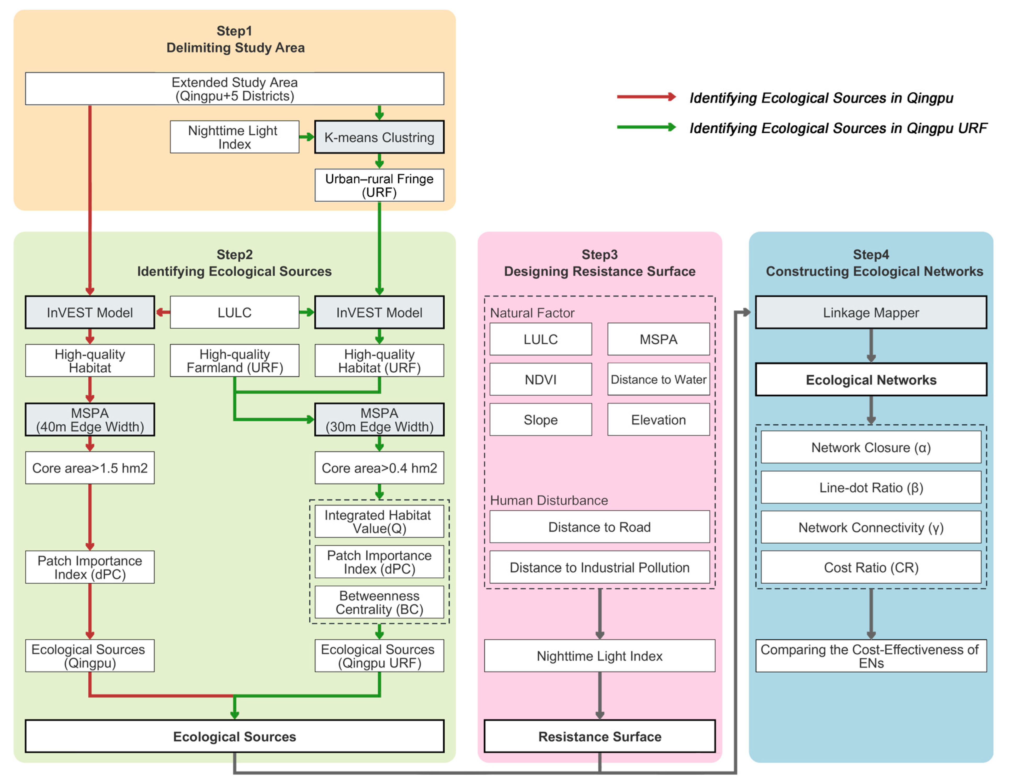
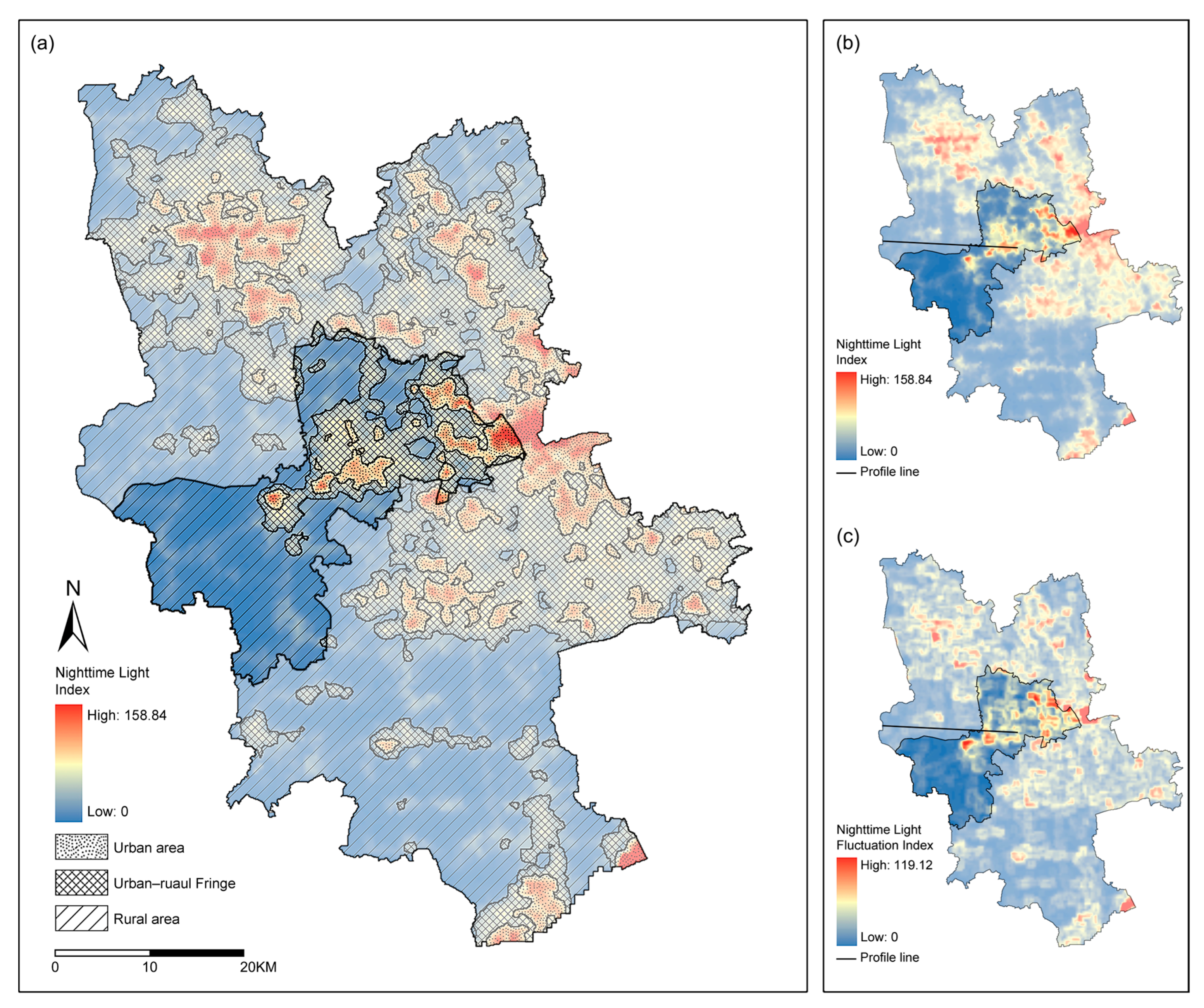
3.1. Delimiting the URF

The night-time light brightness index (DN) and variation index (DN_FI) indicate the intensity of human activity and correlates positively with a region’s urbanization level and population density [43]. We extracted the DN and DN_FI using the Spatial Analysis tool of ArcGIS. The DN_FI can be calculated using Equation (1):

$${DN}_{FI}={DN}_{max}-{DN}_{min},$$

(1)

where ${DN}_{FI}$ represents the degree of change in light brightness, ${DN}_{max}$ and ${DN}_{min},$ respectively, represent the maximum and minimum values of night-time light brightness within a 3 × 3-pixel adjacent area.

By delineating a rural–URF–urban profile line, we analyzed 175 sample points, capturing the transitional fluctuation of brightness and variation (Appendix A, Figure A1). This analysis revealed that rural areas exhibited low brightness and variation, urban areas showed high brightness and low variation, while URFs displayed medium brightness and high variation. Thus, the differentiation in night-time light characteristics proved crucial for identifying URFs [44]. To precisely identify URFs through clustering results based on these characteristics (Figure 3), we employed k-means clustering to maximize intra-group similarity and minimize inter-group differences [45,46]. Consequently, this approach allowed us to accurately delineate the total areas for rural, URF, and urban segments, which were calculated as 1774.13 km², 1333.59 km², and 527.09 km², constituting 48.81%, 36.69%, and 14.50% of the study area, respectively (Appendix A,

Table A1. Clustering results of night-time light indices across rural, urban–rural fringe, and urban areas.

Clustering Results	Urban	Urban–Rural Fringe	Rural
Cluster center of DN	39.01	21.30	5.75
Max DN	158.84	35.94	17.47
Min DN	13.37	4.80	0
Cluster center of DNFI	15.12	22.82	5.64
Max DNFI	56.87	119.12	24.56
Min DNFI	2.27	3.80	0
Number of Samples	53,049	132,931	177,501
Area (km2)	527.09	1333.59	1774.13
Percentage	14.50%	36.69%	48.81%

).

3.2. Identifying Ecological Sources

3.2.1. Identification of High-Value Habitats in Six Districts

(1)

Habitat Quality Assessment Using the InVEST Model

Our study used the Habitat Quality module of the InVEST model to assess habitat quality, which indicates an ecosystem’s ability to support organism survival and biodiversity [47,48]. This module establishes habitat suitability parameters for various land uses and quantifies the impact of anthropogenic threats on habitat degradation. Roads and construction land are identified as the main threat factors. According to the InVEST model user manual [49,50], we set the parameters for these threat factors (

Table 1. Threat factors’ parameter table.

Threat Factors		Influence Distances/km	Weights	Decay
Road	Expressway	3	1	Linear
	Main road	1	0.7	Linear
	Secondary main road	0.5	0.3	Linear
Construction land	Industrial land	10	0.8	Exponential
	Residential land	5	0.6	Exponential
	Other construction land	3	0.5	Exponential

). Higher-grade roads have a broader and more significant impact on habitat quality, with influence distances decreasing from 3 to 0.5 and corresponding weights from 1 to 0.3 [49]. Similarly, the impact of industrial, residential, and other construction land varies, reflected in the decreasing influence distances and weights.

We adjusted suitability values and sensitivity to threat factors (

Table 2. Habitat suitability and its sensitivity to threat factors.

Land Use/Land Cover	Habitat Suitability	Threat Factors
		Road			Construction Land
		Expressway	Main Road	Secondary Main Road	Industrial Land	Residential Land	Other Construction Land
Forest	1	0.5	0.3	0.1	1	0.2	0.2
Bush	0.7	0.6	0.5	0.3	1	0.2	0.2
Grass	0.5	0.8	0.7	0.5	1	0.2	0.2
Paddy field	0.6	0.6	0.5	0.1	1	0.2	0.1
Dry land	0.3	0.3	0.2	0.1	1	0.2	0.1
River	0.8	0.5	0.3	0.2	0.9	0.5	0.3
Lake	1	0.4	0.3	0.2	0.9	0.5	0.3
Pond	0.7	0.4	0.3	0.2	0.8	0.5	0.3
Wetland	0.9	0.6	0.4	0.3	0.9	0.5	0.3
Other Construction land	0	0	0	0	0	0	0
Bare land	0.1	0	0	0	0.3	0	0

), scaled from 0 to 1, to reflect each LULC type’s ecological contribution, based on findings from existing research [51,52]. For paddy fields, a primary habitat type for species in the study region, we set higher habitat suitability at 0.6 and greater sensitivity to expressway and main roads compared to dry land. The assessment results were classified into five levels using the natural breaks method, with the top two levels designated as MSPA foreground [53,54,55].

(2)

Core Areas Extraction Using MSPA

MSPA, based on mathematical morphology principles, is a method for measuring and segmenting image spatial patterns [56,57], capable of identifying seven non-overlapping landscape types at the pixel level, namely core, islet, perforation, edge, bridge, loop, and branch, among which core areas are a key indicator for identifying ecological sources [58].

In MSPA analysis, core areas’ size and number are significantly influenced by the selection of edge width [59]. Thus, we analyzed the impact of different edge widths on landscape segmentation. A 20 m edge width revealed extensive core area distribution but lacked landscape type diversity, while a 60 m edge width fragmented the habitat excessively. A balance was achieved with a 40 m edge width, enabling an optimal representation of landscape types and ensuring connectivity, which met this study’s requirements (Appendix A, Figure A2).

This study established a 1.5 hm² minimum area threshold for core areas after analyzing how increasing thresholds affected the number of core patches. Beyond this threshold, reductions in patch numbers became marginal. Patches under 1.5 hm² constituted only 4.02% of total core area, justifying their exclusion to avoid fragmented patches.

(3)

High-Value Habitat Identification through Patch Connectivity Analysis

Finally, core areas were assessed using the Patch Importance Index, specifically the Potential Connectivity Index (PC) and the Patch Importance Index (dPC), to identify high-value habitats. These indices measure a habitat’s contribution to ecosystem connectivity and integrity [60,61,62]. Based on relevant research [24,63], we set an interconnection threshold of 2500 m and a connectivity probability of 0.5. For patches with dPC values below 4, reductions in patch numbers are marginal. Consequently, core patches with dPC values over 4, which constitute only 1.16% of the total core area, were classified as high-value habitats due to their scarcity.

$$PC=\frac{{\sum }_{i=1}^n{\sum }_{j=1}^n{a}_i{a}_j{p}_{ij}^{\mathrm{*}}}{A_L^2},$$

(2)

$$dPC\left(\mathrm{\%}\right)=\frac{PC-P{C}^{\prime }}{PC}\times 100,$$

(3)

In the formulas, $n$ represents the total number of patches within the study area; $a_i$ and $a_j$, respectively, denote the areas of patch $i$ and patch $j$; $A_L$ is the total area of the study patches; $p_{ij}^{\mathrm{*}}$ is the maximum connectivity probability between patch $i$ and patch $j$; $PC$ is the Potential Connectivity Index of the entire ecological network; and $P{C}^{\prime }$ is the index value after the removal of that patch.

3.2.2. Identification of High-Value URF Habitats in Qingpu District

(1)

Core Areas Extraction Using MSPA

In the URF, farmlands, ponds, and scattered woodlands play a crucial role in biodiversity and ecosystem services provision [11,64]. However, the high- and moderately high-quality habitats identified by the InVEST model within the URF are primarily rivers and woodlands, with farmlands largely overlooked. To address this oversight, we incorporated Dong’s evaluation of Qingpu’s farmland quality, which considers ecological, production, and recreational functions [65], into the MSPA foreground.

Given the influence of edge width on core area extraction, as discussed in Section 3.2.1, we assessed MSPA results under various edge widths (Appendix A, Figure A3). With a 30 m edge width, rivers primarily functioned as bridge areas, enhancing connectivity between URF habitats. Core area patches in the highly urbanized eastern and northern regions showed minimal fragmentation and maintained favorable shapes. Additionally, we established a minimum area threshold of 0.4 hm² for core area patches. Beyond this threshold, the reduction in the number of core patches stabilized, with patches smaller than 0.4 hm² contributing only 1.23% to the total core area.

(2)

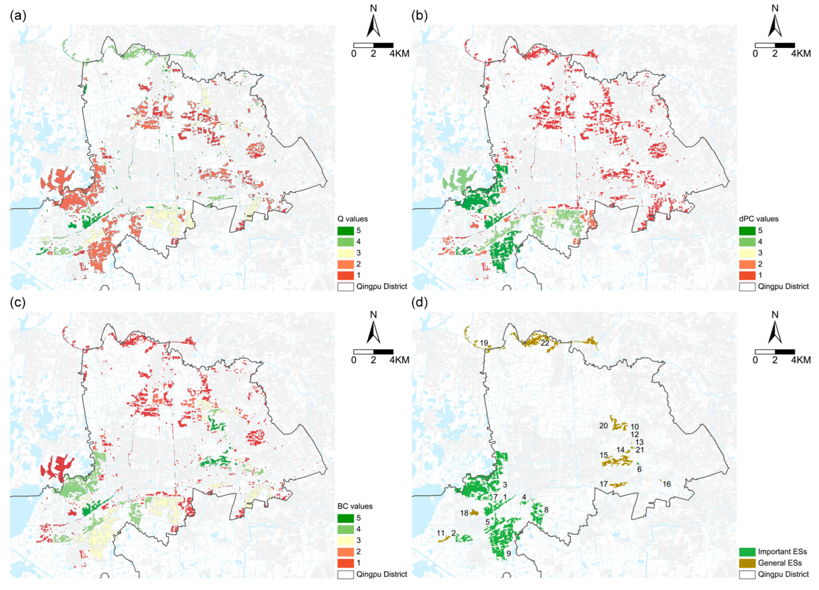
High-Value URF Habitats Identification Based on a Comprehensive Evaluation System

To shelter high-value URF habitats from the core areas, we established a comprehensive evaluation system. This system integrates key metrics such as Integrated Habitat Value (Q), Patch Importance Index (dPC), and Betweenness Centrality Index (BC), reflecting the dual principal functions of URF habitats.

The integrated habitat value (Q) (Appendix A, Figure A4d) for each patch was evaluated using three factors: ecosystem service value (Q1), NDVI (Q2), and habitat quality (Q3). Q was obtained via a grid product operation, with Q1 as the base and Q2 and Q3 as coefficients [24]. The Q can be calculated using Equation (4):

$$Q=Q_1\times Q_2\times Q_3,$$

(4)

Q1 quantifies the annual average value of various ecosystem services per unit area [66]. Our study calculated biodiversity support services provided by different LULC types using the standard equivalence factors defined by Xie et al. (2015) [67] (Appendix A,

Table A2. Biodiversity support service value per unit area for each Land Use/Land Cover.

Land Use/Land Cover	Equivalent Value per Unit Area/1012 Yuan
Forest	2.60
Bush	1.57
Grass	1.27
Paddy field	0.21
Dry land	0.13
Lake	2.55
River	2.55
Pond	2.00
Wetland	7.87
Construction Land	0
Bare Land	0.02

, Figure A4a). Q2, scaled from 0 to 1, evaluates vegetation dynamics including cover, growth, biomass, and net primary productivity, serving as a key indicator for analyzing habitat quality (Figure A4b) [68]. Q3, derived from the InVEST model, assesses habitat quality by considering biodiversity threat factors. This value also ranges from 0 to 1, with higher scores indicating better habitat quality (Figure A4c).

The dPC was utilized to assess the significance of patches to the EN connectivity, while the BC quantifies the role of a specific patch in acting as a stepping stone for the movement of species between neighboring patches [42,62,63,64]. The BC can be calculated using Equation (5):

$$BC(k)={\sum }_i{\sum }_j\frac{p(i,k,j)}{p(i,j)}(i\ne k\ne j),$$

(5)

where $i$ and $j$ represent any two different patches in the network; $p(i,j)$ is the total number of shortest paths between patch $i$ and patch $j$; and $p(i,k,j)$ represents the number of the shortest paths between patch $i$ and patch $j$ that pass-through patch $k$.

Using the natural breaks method, Q, dPC, and BC results were categorized into five levels: low, moderately low, medium, moderately high, and high, with scores ranging from 1 to 5, respectively (Appendix A, Figure A5a–c). These scores for Q, dPC, and BC were then equally weighted and summed to calculate the cumulative score for identifying high-value URF habitats.

Given the complexity of URF habitats fulfilling both biodiversity maintenance and network connectivity enhancement functions, habitats exhibiting either function were deemed essential for ecological conservation. Thus, the criteria for selecting high-value URF habitats were delineated as follows:

① Patches must be over 20 hm² to qualify as high-quality habitats, necessary for local species populations [69,70], and should exhibit high or moderately high Q values;

② Patches that significantly enhance connectivity should display high dPC or BC values;

③ Patches functioning as stepping stones should not surpass 20 hm² and must exhibit high or moderately high BC. According to relevant research [13,71], the sizes of stepping stones range from 5 to 20 hm².

Additionally, patches with cumulative scores above 10 were designated as important ecological sources, while those with lower scores were classified as general (Appendix A, Figure A5d). The score of 10 was chosen to balance the proportion of important ecological sources with general ones, as high-value URF habitat scores range from 7 to 15.

3.3. Designing the Resistance Surface

This study selected resistance factors based on the dual influences of natural environments and human activities (

Table 3. Evaluation system of the resistance surface.

Resistance Factors	Classification	Resistance Values	Weights
Land Use/Land Cover	Forest	1	0.25
	Wetland	1
	River	10
	Lake	10
	Pond	20
	Bush	40
	Grass	50
	Paddy field	50
	Dry land	70
	Bare land	90
	Construction land	100
MSPA landscape types	Core	5	0.15
	Bridge	10
	Loop	20
	Branch	30
	Islet	50
	Edge	60
	Perforation	70
Normalized Difference Vegetation Index	>0.7	1	0.10
	0.5–0.7	20
	0.3–0.5	60
	0.1–0.3	80
	<0.1	100
Distances to water	0–50 m	1	0.10
	50–300 m	30
	300–500 m	60
	>500 m	100
Slope	<8°	1	0.05
	8–15°	25
	15–20	50
	25–35°	75
	>35°	100
Elevation	0–20 m	1	0.05
	20–40 m	20
	40–60 m	30
	60–80 m	40
	>80 m	50
Distances to expressways	>2000 m	1	0.10
	1600–2000 m	20
	1200–1600 m	40
	800–1200 m	60
	400–800 m	80
	0–400 m	100
Distances to main roads	>1000 m	1
	800–1000 m	20
	600–800 m	40
	400–600 m	60
	200–400 m	80
	0–200 m	100
Distances to secondary main roads	>400 m	1
	300–400 m	25
	200–300 m	50
	100–200 m	75
	0–100 m	100
Distances to industrial pollution	>1500 m	1	0.10
	1000–1500 m	25
	500–1000 m	50
	100–500 m	75
	<100 m	100

), tailored to the characteristics of highly urbanized areas, particularly URF areas. For natural environments, factors included LULC, MSPA landscape types, NDVI, distance to water bodies, slope, and elevation [27,72]. Specifically, MSPA landscape types were incorporated to refine connectivity assessments: core areas and bridge areas were allocated minimal resistance values of 5 and 10 to aid species migration, while isolated landscape types such as loops, branches, and edges were assigned values up to 100 [34,35].

To address anthropogenic impacts on habitat quality, resistance factors included the distance to graded roads and proximity to industrial pollution. Using Python, data on polluting factories within the study area were processed to determine resistance values based on proximity to these sources [73].

Furthermore, night-time light brightness, representing the intensity of human activities were utilized to calibrate the resistance surface $R_0$ generated by weighting the sum of the eight resistance factors.

$$R^{\mathrm{*}}=\frac{TL{I}_i}{TL{I}_n}\times R_0,$$

(6)

Formula: $R^{*}$ represents the calibrated resistance value; ${TLI}_i$ denotes the night-time light brightness $DN$ value of grid $i$; ${TLI}_n$ is the average night-time light brightness $DN$ value of land use type $n$; and $R_0$ is the resistance value calculated using the resistance surface evaluation system.

3.4. Constructing and Evaluating ENs

Circuit theory has been widely applied in recent years to simulate the movement patterns of species dispersion [74]. The principle involves treating the grid as a conductive surface, and by inputting ecological sources and resistance surfaces, simulating cumulative electrical current values to represent the probability of species dispersing along a specific path. This study utilized the circuit model to generate ecological corridors, thereby constructing an EN.

Furthermore, we adopted indices including the network closure index (α), line–node ratio index (β), network connectivity index (γ), and cost ratio index (CR) (

Table 4. Evaluation indices for ecological networks.

Indexes	Formulas	Meanings
α	$\alpha =\frac{L-V+1}{2V-5}$	The α index calculates the ratio of the actual number of loops to the maximum possible number of loops within the EN, characterizing the degree to which loops are present for species dispersal.
β	$\beta =\frac{L}{V}$	The β index calculates the ratio of the number of corridors to the number of source locations in the EN, measuring the network’s connectivity.
γ	$\gamma =\frac{L}{3(V-2)}$	The γ index calculates the ratio of the number of corridors to the maximum possible number of corridors within the EN, assessing the connectivity of source locations.
CR	$CR=1-\frac{L}{C}$	The CR index describes the cost of corridor construction within the EN.

) to evaluate the initial and optimized ENs [17,75]. Comparing these indices between the two ENs allows us to discern the impact of URF habitats on the cost-effectiveness of ENs [54,76]. Here, L represents the number of corridors, V the number of sources, and C the length of the corridors within the EN [77].

4. Results

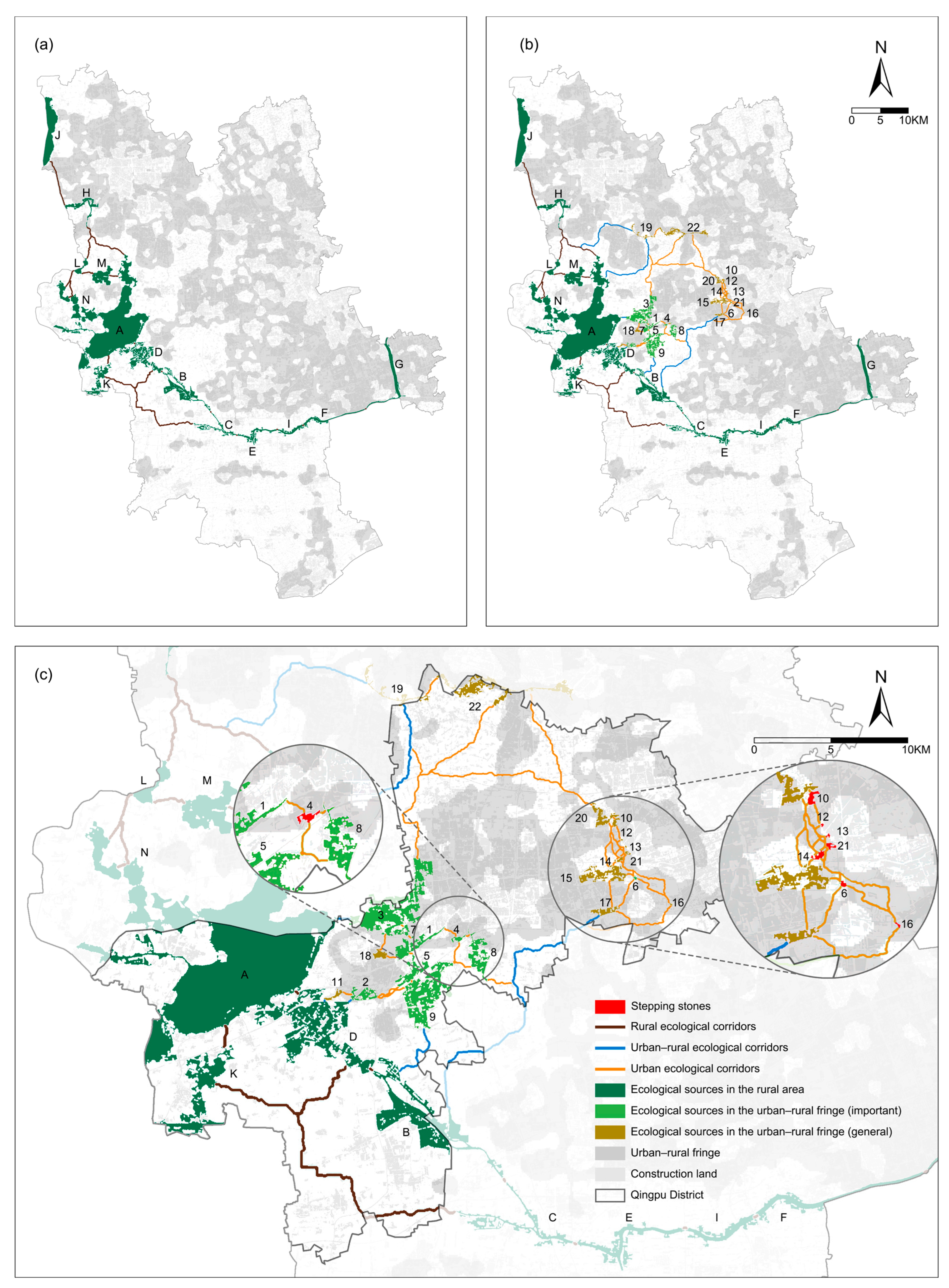
4.1. Results of EN Construction

4.1.1. The Initial EN

Employing the standard method, we identified the initial EN, comprising 14 high-value ecological sources across the study area of six districts (Figure 4a), with sizes ranging from 297.51 to 8276.39 hm² (Appendix A,

Table A3. Land Use/Land Cover areas and percentages of 14 high-value habitats in six districts.

Source	Total Area (hm2)	Area and Percentages of Each LULC (hm2)
		Lake	Pond	River	Bush	Wetland	Forest
A	8276.39	7125.07 (86.09%)	927.82 (11.21%)	87.64 (1.06%)	0.85 (0.01%)	2.04 (0.02%)	133.09 (1.61%)
B	956.46		172.67 (18.05%)	340.71 (35.62%)		2.8 (0.29%)	440.27 (46.03%)
C	306.84			163.43 (53.26%)	0.21 (0.07%)		143.2 (46.67%)
D	1022.20	84.77 (8.29%)	118.8 (11.62%)	116.1 (11.36%)	1.04 (0.1%)	0.22 (0.02%)	701.27 (68.6%)
E	353.68			214.78 (60.73%)	0.04 (0.01%)	0.2 (0.06%)	138.66 (39.2%)
F	353.01			292.63 (82.9%)			60.38 (17.1%)
G	676.46			651.01 (96.24%)			25.45 (3.76%)
H	425.39		179.87 (42.28%)	243.12 (57.15%)			2.4 (0.56%)
I	230.87			155.5 (67.35%)			75.37 (32.65%)
J	1556.10	1509.61 (97.01%)	36.24 (2.33%)	1.39 (0.09%)		0.09 (0.01%)	8.77 (0.56%)
K	580.87	223.95 (38.55%)	148.25 (25.52%)	83.47 (14.37%)			125.2 (21.55%)
L	183.30	94.77 (51.34%)	85.32 (46.22%)	4.5 (2.44%)
M	613.14	407.29 (66.15%)	199.64 (32.42%)	7.87 (1.28%)		0.23 (0.04%)	0.69 (0.11%)
N	297.51	249.18 (83.76%)	48.33 (16.24%)

). In Qingpu District, ecological sources covered a total of 8427.76 hm², representing 27.40% of the district’s total area. The main land use types within these sources are lakes (9694.64 hm², 61.22%), rivers (2362.15 hm², 14.92%), ponds (1916.94 hm², 12.10%), and forests (1854.75 hm², 11.71%), primarily located in the western and central-southern rural areas (Appendix A, Table A3). Notably, no habitats within the URF were classified as high value. Additionally, 18 rural corridors were identified, with 15 located in the western rural areas. Only three corridors, A-H, H-J, and H-L, cross the URF.

4.1.2. The Optimized EN

In addition to the initial EN, this study has developed an optimized method for integrating high-value URF habitats into EN planning. Within the Qingpu’ URF, our integrated habitat value assessment identified 22 high-value sources and subsequently ranked their importance (Figure 4c). We classified 9 sources as important (40.91%) and 13 sources as general (59.09%), as outlined in

Table 5. Comprehensive evaluation and importance grading of the URF sources in Qingpu District.

Source Types	Source Numbers	Area (hm2)	Q	dPC (%)	BC	Q Scores	dPC Scores	BC Scores	Summed Scores
Important sources	1	131.27	1.56	8.02	0.037	5	5	5	15
	2	66.04	1.06	4.69	0.022	4	5	4	13
	3	669.97	0.63	7.00	0.026	2	5	4	11
	4	16.87	0.52	3.62	0.031	2	5	4	11
	5	101.90	0.96	2.59	0.022	3	4	4	11
	6	4.43	1.07	0.00	0.035	4	1	5	10
	7	28.39	1.17	0.82	0.012	4	3	3	10
	8	144.89	0.65	2.06	0.023	2	4	4	10
	9	492.43	0.42	4.65	0.014	2	5	3	10
General sources	10	13.67	0.99	0.02	0.038	3	1	5	9
	11	21.47	1.59	0.37	0.001	5	3	1	9
	12	0.67	0.57	0.00	0.040	2	1	5	8
	13	1.49	0.56	0.03	0.055	2	1	5	8
	14	9.50	0.64	0.03	0.056	2	1	5	8
	15	132.59	0.53	0.06	0.041	2	1	5	8
	16	1.98	0.37	0.02	0.038	2	1	5	8
	17	40.85	1.17	0.01	0.015	4	1	3	8
	18	32.87	2.30	0.13	0.001	5	2	1	8
	19	76.55	1.40	0.02	0.000	5	1	1	7
	20	65.98	0.11	0.06	0.050	1	1	5	7
	21	5.49	0.20	0.03	0.056	1	1	5	7
	22	267.15	1.06	0.08	0.002	4	1	1	6

. Among these 22 sources, 8, including Sources 1, 2, 7, 11, 17, 18, 19, and 22, are characterized as high-quality habitats with an average size of 83.07 hm². Furthermore, eight sources (4, 6, 10, 12, 13, 14, 16, and 21), categorized as having high or moderately high BC value, serve as critical stepping stones with sizes ranging from 0.67 hm² to 16.87 hm² (Table 5; Figure 4c). Notably, the majority of these stepping stones are situated in the highly urbanized areas of northeast Qingpu, facilitating connectivity between rural sources and high-quality URF habitats in the northern and central regions of Qingpu.

Including both rural and URF sources, the optimized EN (Figure 4b) introduced 50 new corridors to the original 18, which includes 7 rural–urban corridors and 43 urban corridors. These corridors, with lengths ranging from 0.11 to 23.67 km and totaling 278.76 km, extend from the rural southwest to central urban areas, forming multiple closed-loop paths around Qingpu New Town (Figure 4c).

4.2. Evaluation of the Cost-Effectiveness of ENs

The structural changes in the initial and optimized ENs in six districts are detailed in

Table 6. Comparison of the initial and optimized ecological network indices.

Indicator	Initial EN	Optimized EN	Change Value
L	18	68	+50
V	14	36	+22
C	80.62	278.76	+198.14
α	0.217	0.493	+0.276
β	1.285	1.889	+0.604
γ	0.500	0.667	+0.167
CR	0.826	0.756	−0.070

. The α and β indices of the optimized EN increased by 127.18% and 47.00%, respectively, compared to the initial EN. This indicates more closed-loop paths have been formed between urban and rural areas, resulting in a more intricate network structure. Additionally, the γ index increased from 0.500 to 0.667, signifying enhanced connectivity between ecological sources. The CR index also showed a slight reduction from 0.826 to 0.756, reflecting a lower construction cost per corridor.

5. Discussion

5.1. A Tailored Method for Identifying High-Value UFR Habitats

URF habitats are crucial for sustaining biodiversity and enhancing connectivity across urban–rural gradients. However, urban expansion fragments these habitats, disrupts ecological processes, isolates corridors [7,9,78], and increases risks of phenomena such as urban heat islands and biodiversity loss [41]. These issues highlight the need for strategic EN planning to mitigate urban expansion impacts and preserve URF habitat functions [10]. Despite their importance, current research often focuses on large-scale rural habitats in rural settings [40,79], overlooking the unique challenges of identifying and evaluating URF habitats [4,11].

Only a few studies have discussed the ecological importance of URF habitats and approaches for their identification, such as the cases in Xiamen city [41], Licheng District in Jinan city [69], and Minhang District in Shanghai [29]. However, these studies have limitations, including ignoring URF habitats’ integrity, neglecting small but high-value habitats, and overlooking their function as stepping stones. These findings underscore the need for a more nuanced approach to URF habitat evaluation that considers both size and functional importance. In response to these challenges, our study developed a tailored method for ensuring the integrity of and assessing high-value URF habitats, thereby making a substantial contribution to EN research.

Accurate delineation of URF boundaries is essential for maintaining the integrity of URF habitats. Traditional methods commonly use criteria such as the proportion of construction land [41] or buffer zones of certain widths [69] to define URFs. However, these methods often overlook the dynamic nature, mixed habitat composition, and land use heterogeneity of URFs, disregarding their actual patterns. In contrast, night-time light data effectively represent urbanization intensity and land use patterns [78,80,81]. Our study demonstrated that differentiating night-time light characteristics, specifically medium brightness and high variation, is crucial for identifying URFs, as evident in Figure A1 in Appendix A. Using k-means clustering, we accurately delineated rural, URF, and urban segments, ensuring a comprehensive and precise identification process.

To further address these challenges, our study introduced an integrated habitat value index (Q) that evaluates URF habitat quality through ecological potential, vegetation coverage, and human disturbance intensity. Enhanced by integrating Betweenness Centrality (BC) [42,82,83] with the Patch Importance Index (dPC), our approach improves connectivity analysis and identifies critical habitats serving as stepping stones. This comprehensive framework addresses previous study limitations by accommodating land use heterogeneity and the specific ecological roles of URF habitats.

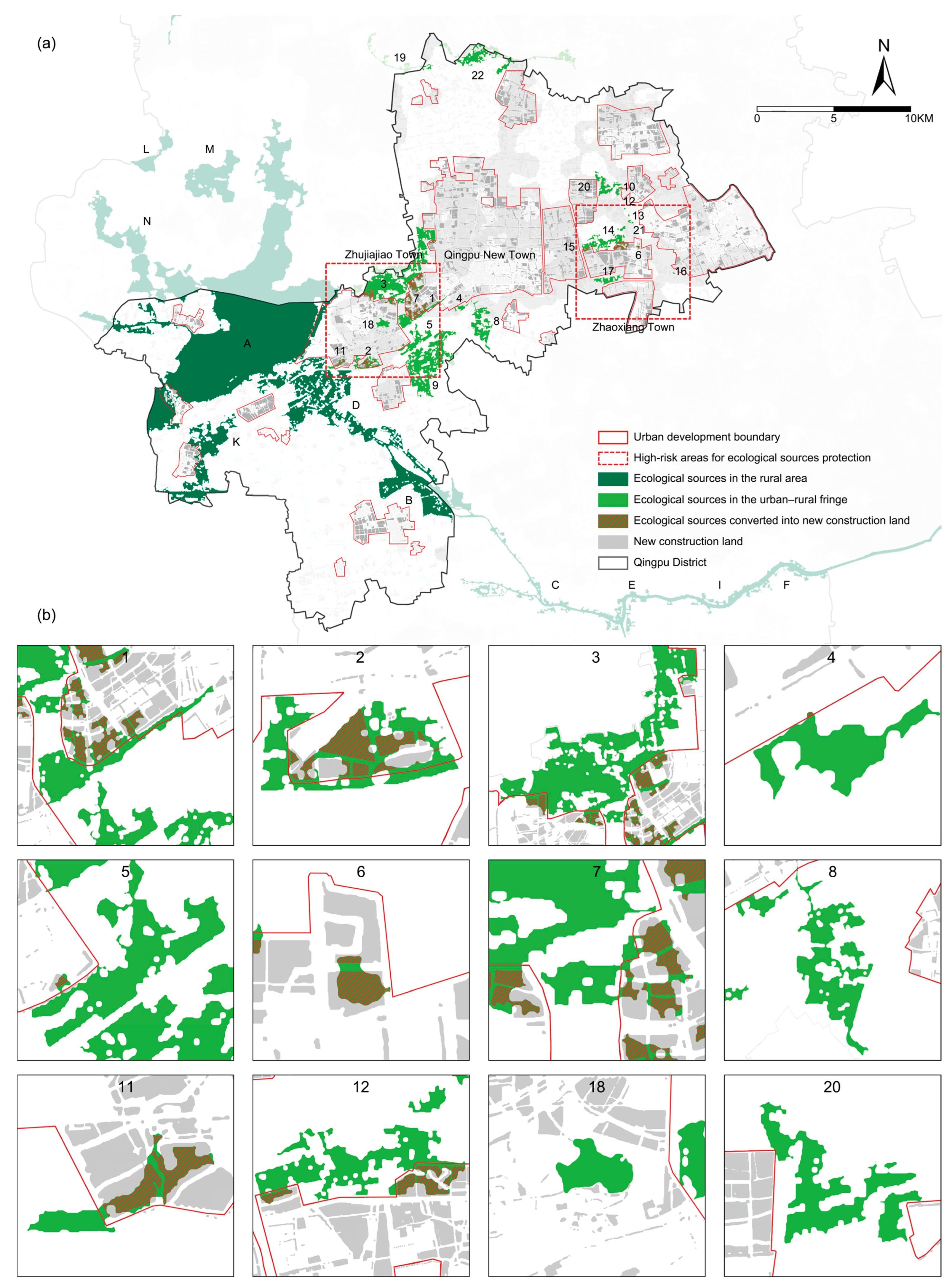
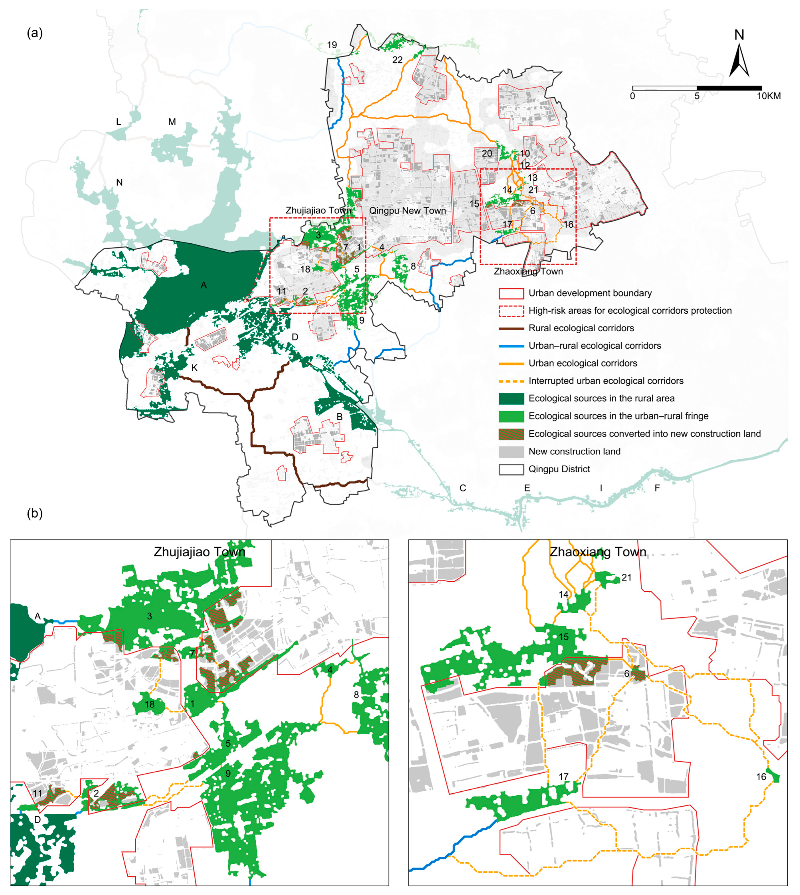
5.2. URF Habitat Protection through Coordinated EN Construction and Territorial Planning

URF habitats, often overlooked due to their abundance and fragmented nature, face significant challenges in territorial protection [84,85]. However, the European Union’s integration of High Nature Value farmland conservation into its rural development assessment framework has effectively protected High Nature Value farmlands and adjacent vegetation within URFs [12,86]. Drawing inspiration from such international practices, this study evaluated the effectiveness of China’s “Three Zones and Three Lines” territorial planning in protecting URF habitats in Qingpu District. Alarmingly, only 21.82% of identified high-value URF habitats are covered by the ecological and permanent basic farmland protection red lines (Figure 5), highlighting a major gap in the legal safeguarding of URF habitats.

The analysis of future urban land use plans within urban development boundaries indicates a significant trend towards converting URF habitats into construction land. Specifically, 12 URF sources, constituting 56.78% of the total, which cover an area of 277.90 hm², are slated for conversion (Figure 6b, marked in hatch brown). This conversion predominantly occurs in Zhujiajiao Town and Zhaoxiang Town, identifying these locations as high-risk areas for habitat loss (Figure 6a). Such conversion threatens the integrity of associated corridors, with 37.21% of urban and 28.57% of urban–rural corridors at high risk of interruption (Figure 7a). The disruption will significantly disrupt ecological connectivity between the northern and central regions of Qingpu.

Notably, in Zhujiajiao Town, over half of the area of the critical habitats, such as sources 1, 2, 7, and 11, which consist of forests and paddy fields vital for local species, are slated for urban development (Figure 6b). This jeopardizes critical urban corridors like 1–4, 1–7, 1–18, 2–5, 2–9, and 2–11 and significantly affects urban–rural corridors like 2-D and 11-D. In Zhaoxiang Town, the near-total conversion of the stepping stone source 6 will disrupt five urban corridors: 6–14, 6–15, 6–16, 6–17, and 6–21 (Figure 7b). Proactive measures are necessary to mitigate these impacts. Restoring source 6 and its five connected corridors, protecting sources 1 and 7 across development boundaries, and preserving sources 2 and 11 adjacent to the high-quality source D are essential steps to sustain urban–rural connectivity and maintain ecological stability.

5.3. Limitations and Future Research Directions

This study encountered several limitations regarding the selection of indicators for identifying high-value URF habitats, integrating URF habitat protection into statutory planning, and targeting focal species in EN construction.

(1)

Indicator Selection

Our analysis primarily utilized habitat area, quality, and connectivity to identify high-value URF habitats. However, future research should expand these criteria to include patch shape complexity [87], dispersal capabilities of focal species [13,88], and the quality of adjacent habitats, such as natural vegetation coverage and land use intensity [84]. These expanded indicators are essential for a more comprehensive evaluation of URF habitat’s integrity and ecological value;

(2)

Integration into Territorial Planning

To effectively integrate URF habitat protection into China’s territorial planning, conducting robustness analyses is recommended. These analyses are crucial for assessing the impacts of URF habitat removal on the stability of ENs and provide a clear visualization of the consequences of habitat encroachment, highlighting areas for urgent policy intervention and management [82,89]. Furthermore, effective integration should also focus on enhancing the connections between high-value URF habitats and the broader network of high-value rural and urban habitats [11]. Future research should identify strategic locations within the URF that could be transformed into ecological sources, significantly enhancing the connectivity of the overall network and optimizing the regional ecological protection pattern, thus facilitating a seamless integration of urban and rural environments [41,90,91].

(3)

Species-Specific Focus

The general approach of our study led to broad threshold settings due to a lack of species-specific focus. Concentrating on particular species would enable a more precise analysis of LULC-based habitat quality assessment [42,83] and allow for consideration of species-specific permeability when setting resistance values. This focus will align conservation efforts more closely with ecological needs, resulting in more effective habitat management.

6. Conclusions

Aiming to protect URF habitats in the face of rapid urbanization, this study aimed to integrate ecologically valuable URF habitats into EN construction and territorial planning for coordinated protection. Employing Shanghai’s Qingpu District as a case study, we devised a methodology to identify high-value URF habitats and connect them with large-scale, high-quality habitats in rural settings within an EN, thereby enhancing species movement across urban and rural environments. Our findings reveal that:

(1) The initial EN recognized only 14 sources and 18 corridors predominantly in rural areas, with no URF habitats classified as high value. Overlooking the ecological contributions of URF habitats has led to a lack of ecological sources and corridors in the highly urbanized northeastern areas, significantly limiting species dispersal between urban and rural areas;

(2) Our optimized approach highlighted the unique characteristics and ecological value of URF habitats. We identified 22 URF sources and added 50 new urban and urban–rural corridors, extending from the southwestern rural areas to the central urban regions. This expansion created multiple closed-loop paths around Qingpu New Town, effectively facilitating species dispersal and reconnecting disrupted ecological processes;

(3) The optimized EN demonstrated increased cost-effectiveness, significantly improving connectivity indices (α by 127.18%, β by 47.00%, and γ by 33.4%) while decreasing construction costs (CR index by 0.07). These results highlight that integrating URF habitats into the ecological conservation framework enhanced connectivity at a reduced cost;

(4) The existing “Three Zones and Three Lines” policy has failed to safeguard URF habitats, endangering 56.78% of high-quality habitats and crucial stepping stones. This failure threatens 37.21% of urban and 28.57% of urban–rural corridors, disrupting ecological connectivity between northern and central Qingpu. Proactive measures are necessary to restore source 1, 2, 6, 7, and 11 and their connected 13 corridors to sustain urban–rural connectivity.

In conclusion, this study highlights the significance of URF habitats within ENs and advances EN construction methodologies. It delivers empirical support and offers policy recommendations for safeguarding these habitats under Qingpu District’s territorial planning framework, serving as a pertinent model for regions undergoing similar urbanization.

References

1. Allen, A. Environmental planning and management of the peri-urban interface: Perspectives on an emerging field. Environ. Urban. 2003, 15, 135–148. [Google Scholar] [CrossRef]
2. González, C. Evolution of the concept of ecological integrity and its study through networks. Ecol. Model. 2023, 476, 110224. [Google Scholar] [CrossRef]
3. Li, J.; Gao, J.; Zhang, X.; Zheng, X. Effects of urbanization on biodiversity: A review. Chin. J. Ecol. 2005, 24, 953–957. [Google Scholar] [CrossRef]
4. Tang, X.; Xing, Z. Research on Construction of Greenbelt Around a City Integrating Protection of Semi-natural Habitats in Urban Fringe. Landsc. Archit. 2021, 28, 90–95. [Google Scholar] [CrossRef]
5. Zerbe, S.; Maurer, U.; Schmitz, S.; Sukopp, H. Biodiversity in Berlin and its potential for nature conservation. Landsc. Urban Plan. 2003, 62, 139–148. [Google Scholar] [CrossRef]
6. Haregeweyn, N.; Fikadu, G.; Tsunekawa, A.; Tsubo, M.; Meshesha, D.T. The dynamics of urban expansion and its impacts on land use/land cover change and small-scale farmers living near the urban fringe: A case study of Bahir Dar, Ethiopa. Landsc. Urban Plan. 2012, 106, 149–157. [Google Scholar] [CrossRef]
7. Allan, J.R.; Possingham, H.P.; Atkinson, S.C.; Waldron, A.; Di Marco, M.; Butchart, S.H.M.; Adams, V.M.; Kissling, W.D.; Worsdell, T.; Sandbrook, C.; et al. The minimum land area requiring conservation attention to safeguard biodiversity. Science 2022, 376, 1094–1101. [Google Scholar] [CrossRef] [PubMed]
8. Ma, W.; Jiang, G.; Chen, Y.; Qu, Y.; Zhou, T.; Li, W. How feasible is regional integration for reconciling land use conflicts across the urban–rural interface? Evidence from Beijing–Tianjin–Hebei metropolitan region in China. Land Use Policy 2020, 92, 104433. [Google Scholar] [CrossRef]
9. Wang, S.; Wu, M.; Hu, M.; Fan, C.; Wang, T.; Xia, B. Promoting landscape connectivity of highly urbanized area: An ecological network approach. Ecol. Indic. 2021, 125, 107487. [Google Scholar] [CrossRef]
10. Shen, J.; Zhu, W.; Peng, Z.; Wang, Y. Improving landscape ecological network connectivity in urbanizing areas from dual dimensions of structure and function. Ecol. Model. 2023, 482, 110380. [Google Scholar] [CrossRef]
11. Tang, X. The Protection Planning of Small and Micro Habitats in Urban Fringe Areas: Enlightenment from the Management of High Natural Value Farmland in the EU to the Maintenance of Biodiversity in Urban Areas in China. Urban Plan. Int. 2021, 36, 74–116. [Google Scholar] [CrossRef]
12. Schmitz, M.F.; Arnaiz-Schmitz, C.; Sarmiento-Mateos, P. High Nature Value Farming Systems and Protected Areas: Conservation Opportunities or Land Abandonment? A Study Case in the Madrid Region (Spain). Land 2021, 10, 721. [Google Scholar] [CrossRef]
13. Han, L.; Wang, Z.; Wei, M.; Wang, M.; Shi, H.; Ruckstuhl, K.; Yang, W.; Alves, J. Small patches play a critical role in the connectivity of the Western Tianshan landscape, Xinjiang, China. Ecol. Indic. 2022, 144, 109542. [Google Scholar] [CrossRef]
14. McGarigal, K.; Cushman, S.A. Comparative Evaluation of Experimental Approaches To the Study of Habitat Fragmentation Effects. Ecol. Appl. 2002, 12, 335–345. [Google Scholar] [CrossRef]
15. Saura, S.; Estreguil, C.; Mouton, C.; Rodríguez-Freire, M. Network analysis to assess landscape connectivity trends: Application to European forests (1990–2000). Ecol. Indic. 2011, 11, 407–416. [Google Scholar] [CrossRef]
16. Szangolies, L.; Rohwäder, M.-S.; Jeltsch, F. Single large AND several small habitat patches: A community perspective on their importance for biodiversity. Basic Appl. Ecol. 2022, 65, 16–27. [Google Scholar] [CrossRef]
17. Wang, H.; Gao, Y.; Li, Y.; Li, N.; Grueter, C.C.; Xu, H.; Huang, Z.; Cui, L.; Xiao, W. Stepping Stone Strategy: A Cost-Effective Way to Address Habitat Fragmentation of Endangered Wildlife in Montane Forest. Ecosyst. Health Sustain. 2023, 9, 0073. [Google Scholar] [CrossRef]
18. Fletcher, R.J.; Didham, R.K.; Banks-Leite, C.; Barlow, J.; Ewers, R.M.; Rosindell, J.; Holt, R.D.; Gonzalez, A.; Pardini, R.; Damschen, E.I.; et al. Is habitat fragmentation good for biodiversity? Biol. Conserv. 2018, 226, 9–15. [Google Scholar] [CrossRef]
19. Leroux, S.J.; Schmiegelow, F.K.A.; Lessard, R.B.; Cumming, S.G. Minimum dynamic reserves: A framework for determining reserve size in ecosystems structured by large disturbances. Biol. Conserv. 2007, 138, 464–473. [Google Scholar] [CrossRef]
20. Li, F.; Ye, Y.; Song, B.; Wang, R. Evaluation of urban suitable ecological land based on the minimum cumulative resistance model: A case study from Changzhou, China. Ecol. Model. 2015, 318, 194–203. [Google Scholar] [CrossRef]
21. Griffiths, M.B. Lamb Buddha’s Migrant Workers: Self-Assertion on China’s Urban Fringe. J. Curr. Chin. Aff. 2010, 39, 3–37. [Google Scholar] [CrossRef]
22. Liu, X.; Li, X.; Zhang, Y.; Wang, Y.; Chen, J.; Geng, Y. Spatiotemporal evolution and relationship between construction land expansion and territorial space conflicts at the county level in Jiangsu Province. Ecol. Indic. 2023, 154, 110662. [Google Scholar] [CrossRef]
23. Zhang, J.; Chen, Y.; Zhu, C.; Huang, B.; Gan, M. Identification of Potential Land-Use Conflicts between Agricultural and Ecological Space in an Ecologically Fragile Area of Southeastern China. Land 2021, 10, 1011. [Google Scholar] [CrossRef]
24. Zhang, R.; Zhang, Q.; Zhang, L.; Zhong, Q.; Liu, J.; Wang, Z. Identification and extraction of a current urban ecological network in Minhang District of Shanghai based on an optimization method. Ecol. Indic. 2022, 136, 108647. [Google Scholar] [CrossRef]
25. Ignatieva, M.; Stewart, G.H.; Meurk, C. Planning and design of ecological networks in urban areas. Landsc. Ecol. Eng. 2010, 7, 17–25. [Google Scholar] [CrossRef]
26. Jongman, R.H.; Külvik, M.; Kristiansen, I. European ecological networks and greenways. Landsc. Urban Plan. 2004, 68, 305–319. [Google Scholar] [CrossRef]
27. Huang, L.; Wang, J.; Fang, Y.; Zhai, T.; Cheng, H. An integrated approach towards spatial identification of restored and conserved priority areas of ecological network for implementation planning in metropolitan region. Sustain. Cities Soc. 2021, 69, 102865. [Google Scholar] [CrossRef]
28. Xu, A.; Hu, M.; Shi, J.; Bai, Q.; Li, X. Construction and optimization of ecological network in inland river basin based on circuit theory, complex network and ecological sensitivity: A case study of Gansu section of Heihe River Basin. Ecol. Model. 2024, 488, 110578. [Google Scholar] [CrossRef]
29. Zhang, R.; Zhang, L.; Zhong, Q.; Zhang, Q.; Ji, Y.; Song, P.; Wang, Q. An optimized evaluation method of an urban ecological network: The case of the Minhang District of Shanghai. Urban For. Urban Green. 2021, 62, 127158. [Google Scholar] [CrossRef]
30. Aslan, C.E.; Brunson, M.W.; Sikes, B.A.; Epanchin-Niell, R.S.; Veloz, S.; Theobald, D.M.; Dickson, B.G. Coupled ecological and management connectivity across administrative boundaries in undeveloped landscapes. Ecosphere 2021, 12, e03329. [Google Scholar] [CrossRef]
31. Liu, X.; Li, X.; Yang, J.; Fan, H.; Zhang, J.; Zhang, Y. How to resolve the conflicts of urban functional space in planning: A perspective of urban moderate boundary. Ecol. Indic. 2022, 144, 109495. [Google Scholar] [CrossRef]
32. Liu, H.; Niu, T.; Yu, Q.; Yang, L.; Ma, J.; Qiu, S.; Wang, R.; Liu, W.; Li, J. Spatial and temporal variations in the relationship between the topological structure of eco-spatial network and biodiversity maintenance function in China. Ecol. Indic. 2022, 139, 108919. [Google Scholar] [CrossRef]
33. Zhao, H.; He, J.; Liu, D.; Han, Y.; Zhou, Z.; Niu, J. Incorporating ecological connectivity into ecological functional zoning: A case study in the middle reaches of Yangtze River urban agglomeration. Ecol. Inform. 2023, 75, 102098. [Google Scholar] [CrossRef]
34. Wang, Y.; Qu, Z.; Zhong, Q.; Zhang, Q.; Zhang, L.; Zhang, R.; Yi, Y.; Zhang, G.; Li, X.; Liu, J. Delimitation of ecological corridors in a highly urbanizing region based on circuit theory and MSPA. Ecol. Indic. 2022, 142, 109258. [Google Scholar] [CrossRef]
35. Wei, Q.; Halike, A.; Yao, K.; Chen, L.; Balati, M. Construction and optimization of ecological security pattern in Ebinur Lake Basin based on MSPA-MCR models. Ecol. Indic. 2022, 138, 108857. [Google Scholar] [CrossRef]
36. Donati, G.F.; Bolliger, J.; Psomas, A.; Maurer, M.; Bach, P.M. Reconciling cities with nature: Identifying local Blue-Green Infrastructure interventions for regional biodiversity enhancement. J. Environ. Manag. 2022, 316, 115254. [Google Scholar] [CrossRef]
37. Reza, M.I.H.; Rafaai, N.H.; Abdullah, S.A. Application of graph-based indices to map and develop a connectivity importance index for large mammal conservation in a tropical region: A case study in Selangor State, Peninsular Malaysia. Ecol. Indic. 2022, 140, 109008. [Google Scholar] [CrossRef]
38. Chen, H.; Yan, W.; Li, Z.; Wende, W.; Xiao, S.; Wan, S.; Li, S. Spatial patterns of associations among ecosystem services across different spatial scales in metropolitan areas: A case study of Shanghai, China. Ecol. Indic. 2022, 136, 108682. [Google Scholar] [CrossRef]
39. Huang, Z.; Qian, L.; Cao, W. Developing a Novel Approach Integrating Ecosystem Services and Biodiversity for Identifying Priority Ecological Reserves. Resour. Conserv. Recycl. 2021, 179, 106128. [Google Scholar] [CrossRef]
40. Yang, Y.; Feng, Z.; Wu, K.; Lin, Q. How to construct a coordinated ecological network at different levels: A case from Ningbo city, China. Ecol. Inform. 2022, 70, 101742. [Google Scholar] [CrossRef]
41. Liang, C.; Zeng, J.; Zhang, R.-C.; Wang, Q.-W. Connecting urban area with rural hinterland: A stepwise ecological security network construction approach in the urban-rural fringe. Ecol. Indic. 2022, 138, 108794. [Google Scholar] [CrossRef]
42. Lumia, G.; Praticò, S.; Di Fazio, S.; Cushman, S.; Modica, G. Combined use of urban Atlas and Corine land cover datasets for the implementation of an ecological network using graph theory within a multi-species approach. Ecol. Indic. 2023, 148, 110150. [Google Scholar] [CrossRef]
43. Li, X.; Zhou, Y. Urban mapping using DMSP/OLS stable night-time light: A review. Int. J. Remote Sens. 2017, 38, 6030–6046. [Google Scholar] [CrossRef]
44. Feng, Z.; Peng, J.; Wu, J. Using DMSP/OLS nighttime light data and K–means method to identify urban–rural fringe of megacities. Habitat Int. 2020, 103, 102227. [Google Scholar] [CrossRef]
45. Small, C.; Pozzi, F.; Elvidge, C. Spatial analysis of global urban extent from DMSP-OLS night lights. Remote Sens. Environ. 2005, 96, 277–291. [Google Scholar] [CrossRef]
46. Ding, W.; Chen, H. Urban-rural fringe identification and spatial form transformation during rapid urbanization: A case study in Wuhan, China. Build. Environ. 2022, 226, 109697. [Google Scholar] [CrossRef]
47. Peng, J.; Pan, Y.; Liu, Y.; Zhao, H.; Wang, Y. Linking ecological degradation risk to identify ecological security patterns in a rapidly urbanizing landscape. Habitat Int. 2018, 71, 110–124. [Google Scholar] [CrossRef]
48. Terrado, M.; Sabater, S.; Chaplin-Kramer, B.; Mandle, L.; Ziv, G.; Acuña, V. Model development for the assessment of terrestrial and aquatic habitat quality in conservation planning. Sci. Total. Environ. 2016, 540, 63–70. [Google Scholar] [CrossRef] [PubMed]
49. Tang, Y.; Gao, C.; Wu, X. Urban Ecological Corridor Network Construction: An Integration of the Least Cost Path Model and the InVEST Model. ISPRS Int. J. Geo-Inf. 2020, 9, 33. [Google Scholar] [CrossRef]
50. Riitters, K.H.; Vogt, P.; Soille, P.; Kozak, J.; Estreguil, C. Neutral model analysis of landscape patterns from mathematical morphology. Landsc. Ecol. 2007, 22, 1033–1043. [Google Scholar] [CrossRef]
51. Goldstein, J.H.; Caldarone, G.; Duarte, T.K.; Ennaanay, D.; Hannahs, N.; Mendoza, G.; Polasky, S.; Wolny, S.; Daily, G.C. Integrating ecosystem-service tradeoffs into land-use decisions. Proc. Natl. Acad. Sci. USA 2012, 109, 7565–7570. [Google Scholar] [CrossRef] [PubMed]
52. Nelson, E.; Mendoza, G.; Regetz, J.; Polasky, S.; Tallis, H.; Cameron, D.; Chan, K.M.A.; Daily, G.C.; Goldstein, J.; Kareiva, P.M.; et al. Modeling multiple ecosystem services, biodiversity conservation, commodity production, and tradeoffs at landscape scales. Front. Ecol. Environ. 2009, 7, 4–11. [Google Scholar] [CrossRef]
53. Sun, H.; Wei, J.; Han, Q. Assessing land-use change and landscape connectivity under multiple green infrastructure conservation scenarios. Ecol. Indic. 2022, 142, 109236. [Google Scholar] [CrossRef]
54. Huang, X.; Wang, H.; Shan, L.; Xiao, F. Constructing and optimizing urban ecological network in the context of rapid urbanization for improving landscape connectivity. Ecol. Indic. 2021, 132, 108319. [Google Scholar] [CrossRef]
55. Zhai, T.; Huang, L. Linking MSPA and Circuit Theory to Identify the Spatial Range of Ecological Networks and Its Priority Areas for Conservation and Restoration in Urban Agglomeration. Front. Ecol. Evol. 2022, 10, 828979. [Google Scholar] [CrossRef]
56. Soille, P.; Vogt, P. Morphological segmentation of binary patterns. Pattern Recognit. Lett. 2008, 30, 456–459. [Google Scholar] [CrossRef]
57. Vogt, P.; Riitters, K. GuidosToolbox: Universal digital image object analysis. Eur. J. Remote Sens. 2017, 50, 352–361. [Google Scholar] [CrossRef]
58. Li, Y.-Y.; Zhang, Y.-Z.; Jiang, Z.-Y.; Guo, C.-X.; Zhao, M.-Y.; Yang, Z.-G.; Guo, M.-Y.; Wu, B.-Y.; Chen, Q.-L. Integrating morphological spatial pattern analysis and the minimal cumulative resistance model to optimize urban ecological networks: A case study in Shenzhen City, China. Ecol. Process. 2021, 10, 63. [Google Scholar] [CrossRef]
59. Zhou, Q.; Bosch, C.C.K.v.D.; Chen, J.; Zhang, W.; Dong, J. Identification of ecological networks and nodes in Fujian province based on green and blue corridors. Sci. Rep. 2021, 11, 20872. [Google Scholar] [CrossRef]
60. Keeley, A.T.; Beier, P.; Jenness, J.S. Connectivity metrics for conservation planning and monitoring. Biol. Conserv. 2021, 255, 109008. [Google Scholar] [CrossRef]
61. Lim, C.H. Establishing an Ecological Network to Enhance Forest Connectivity in South Korea’s Demilitarized Zone. Land 2024, 13, 106. [Google Scholar] [CrossRef]
62. Saura, S.; Pascual-Hortal, L. A new habitat availability index to integrate connectivity in landscape conservation planning: Comparison with existing indices and application to a case study. Landsc. Urban Plan. 2007, 83, 91–103. [Google Scholar] [CrossRef]
63. Zhang, X.; Wang, X.; Zhang, C.; Zhai, J. Development of a cross-scale landscape infrastructure network guided by the new Jiangnan watertown urbanism: A case study of the ecological green integration demonstration zone in the Yangtze River Delta, China. Ecol. Indic. 2022, 143, 109317. [Google Scholar] [CrossRef]
64. Panzacchi, M.; Linnell, J.D.C.; Melis, C.; Odden, M.; Odden, J.; Gorini, L.; Andersen, R. Effect of land-use on small mammal abundance and diversity in a forest–farmland mosaic landscape in south-eastern Norway. For. Ecol. Manag. 2010, 259, 1536–1545. [Google Scholar] [CrossRef]
65. Dong, Y.; Zhao, H. Study on Trade-off and Synergy Relationship of Cultivated Land Multifunction: A Case of Qingpu District, Shanghai. Resour. Environ. Yangtze Basin 2019, 28, 368–375. [Google Scholar]
66. Xie, G.D.; Lu, C.X.; Leng, Y.F.; Zheng, D.U.; Li, S.C. Ecological assets valuation of the Tibetan Plateau. J. Nat. Resour. 2003, 18, 189–196. [Google Scholar]
67. Xie, G.; Zhang, C.; Zhang, L.; Chen, W.; Li, S. Improvement of the Evaluation Method for Ecosystem Service Value Based on Per Unit Area. J. Nat. Resour. 2015, 30, 1243–1254. [Google Scholar] [CrossRef]
68. Wang, Z.; Liu, Z.; Huang, M. NDVI joint process-based models drive a learning ensemble model for accurately estimating cropland net primary productivity (NPP). Front. Environ. Sci. 2024, 11, 1304400. [Google Scholar] [CrossRef]
69. Fan, J.; Wang, Q.; Ji, M.; Sun, Y.; Feng, Y.; Yang, F.; Zhang, Z. Ecological network construction and gradient zoning optimization strategy in urban-rural fringe: A case study of Licheng District, Jinan City, China. Ecol. Indic. 2023, 150, 110251. [Google Scholar] [CrossRef]
70. Mimet, A.; Clauzel, C.; Foltête, J.-C. Locating wildlife crossings for multispecies connectivity across linear infrastructures. Landsc. Ecol. 2016, 31, 1955–1973. [Google Scholar] [CrossRef]
71. Luo, Y.; Wu, J.; Wang, X.; Peng, J. Using stepping-stone theory to evaluate the maintenance of landscape connectivity under China’s ecological control line policy. J. Clean. Prod. 2021, 296, 126356. [Google Scholar] [CrossRef]
72. Dong, J.; Guo, F.; Lin, M.; Zhang, H.; Zhu, P. Optimization of green infrastructure networks based on potential green roof integration in a high-density urban area—A case study of Beijing, China. Sci. Total. Environ. 2022, 834, 155307. [Google Scholar] [CrossRef] [PubMed]
73. Huang, M.-Y.; Yue, W.-Z.; Feng, S.-R.; Cai, J.-J. Analysis of spatial heterogeneity of ecological security based on MCR model and ecological pattern optimization in the Yuexi county of the Dabie Mountain Area. J. Nat. Resour. 2019, 34, 771–784. [Google Scholar] [CrossRef]
74. Liang, G.; Niu, H.; Li, Y. A multi-species approach for protected areas ecological network construction based on landscape connectivity. Glob. Ecol. Conserv. 2023, 46, e02569. [Google Scholar] [CrossRef]
75. Zou, S.; Fan, R.; Gong, J. Spatial Optimization and Temporal Changes in the Ecological Network: A Case Study of Wanning City, China. Land 2024, 13, 122. [Google Scholar] [CrossRef]
76. Nie, W.; Shi, Y.; Siaw, M.J.; Yang, F.; Wu, R.; Wu, X.; Zheng, X.; Bao, Z. Constructing and optimizing ecological network at county and town Scale: The case of Anji County, China. Ecol. Indic. 2021, 132, 108294. [Google Scholar] [CrossRef]
77. Kang, J.; Li, C.; Li, M.; Zhang, T.; Zhang, B. Identifying priority areas for conservation in the lower Yellow River basin from an ecological network perspective. Ecosyst. Health Sustain. 2022, 8, 2105751. [Google Scholar] [CrossRef]
78. Wang, L.; Zhao, J.; Lin, Y.; Chen, G. Exploring ecological carbon sequestration advantage and economic responses in an ecological security pattern: A nature-based solutions perspective. Ecol. Model. 2024, 488, 110597. [Google Scholar] [CrossRef]
79. Shen, Z.; Wu, W.; Chen, S.; Tian, S.; Wang, J.; Li, L. A static and dynamic coupling approach for maintaining ecological networks connectivity in rapid urbanization contexts. J. Clean. Prod. 2022, 369, 133375. [Google Scholar] [CrossRef]
80. Hu, C.; Wang, Z.; Wang, Y.; Sun, D.; Zhang, J. Combining MSPA-MCR Model to Evaluate the Ecological Network in Wuhan, China. Land 2022, 11, 213. [Google Scholar] [CrossRef]
81. Wu, B.; Yang, C.; Wu, Q.; Wang, C.; Wu, J.; Yu, B. A building volume adjusted nighttime light index for characterizing the relationship between urban population and nighttime light intensity. Comput. Environ. Urban Syst. 2023, 99, 101911. [Google Scholar] [CrossRef]
82. Bodin, Ö.; Saura, S. Ranking individual habitat patches as connectivity providers: Integrating network analysis and patch removal experiments. Ecol. Model. 2010, 221, 2393–2405. [Google Scholar] [CrossRef]
83. Modica, G.; Praticò, S.; Laudari, L.; Ledda, A.; Di Fazio, S.; De Montis, A. Implementation of multispecies ecological networks at the regional scale: Analysis and multi-temporal assessment. J. Environ. Manag. 2021, 289, 112494. [Google Scholar] [CrossRef] [PubMed]
84. Wintle, B.A.; Kujala, H.; Whitehead, A.; Cameron, A.; Veloz, S.; Kukkala, A.; Moilanen, A.; Gordon, A.; Lentini, P.E.; Cadenhead, N.C.R.; et al. Global synthesis of conservation studies reveals the importance of small habitat patches for biodiversity. Proc. Natl. Acad. Sci. USA 2019, 116, 909–914. [Google Scholar] [CrossRef] [PubMed]
85. Fahrig, L.; Arroyo-Rodríguez, V.; Bennett, J.R.; Boucher-Lalonde, V.; Cazetta, E.; Currie, D.J.; Eigenbrod, F.; Ford, A.T.; Harrison, S.P.; Jaeger, J.A.G.; et al. Is habitat fragmentation bad for biodiversity? Biol. Conserv. 2019, 230, 179–186. [Google Scholar] [CrossRef]
86. Lomba, A.; Guerra, C.; Alonso, J.; Honrado, J.P.; Jongman, R.; McCracken, D. Mapping and monitoring High Nature Value farmlands: Challenges in European landscapes. J. Environ. Manag. 2014, 143, 140–150. [Google Scholar] [CrossRef] [PubMed]
87. Su, K.; Yu, Q.; Yue, D.; Zhang, Q.; Yang, L.; Liu, Z.; Niu, T.; Sun, X. Simulation of a forest-grass ecological network in a typical desert oasis based on multiple scenes. Ecol. Model. 2019, 413, 108834. [Google Scholar] [CrossRef]
88. da Rocha, G.; Brigatti, E.; Niebuhr, B.B.; Ribeiro, M.C.; Vieira, M.V. Dispersal movement through fragmented landscapes: The role of stepping stones and perceptual range. Landsc. Ecol. 2021, 36, 3249–3267. [Google Scholar] [CrossRef]
89. Luo, Y.; Wu, J.; Wang, X.; Wang, Z.; Zhao, Y. Can policy maintain habitat connectivity under landscape fragmentation? A case study of Shenzhen, China. Sci. Total. Environ. 2020, 715, 136829. [Google Scholar] [CrossRef] [PubMed]
90. Huang, B.-X.; Chiou, S.-C.; Li, W.-Y. Landscape Pattern and Ecological Network Structure in Urban Green Space Planning: A Case Study of Fuzhou City. Land 2021, 10, 769. [Google Scholar] [CrossRef]
91. Kwon, O.-S.; Kim, J.-H.; Ra, J.-H. Landscape Ecological Analysis of Green Network in Urban Area Using Circuit Theory and Least-Cost Path. Land 2021, 10, 847. [Google Scholar] [CrossRef]
Figure 1. Overview of the study area: (a) the land use/land cover (LULC) map in 2020 and the location of Qingpu District and its surrounding five districts; and (b) the comparison of habitat features in the LULC maps originated from four datasets.
Land 13 00935 g001
Figure 2. The framework of this study.
Land 13 00935 g002
Figure 3. (a) Identification results of the urban–rural fringe in six districts; (b) distribution map of the night-time light brightness index (DN) and (c) the variation index (DNFI) in six districts.
Land 13 00935 g003
Figure 4. (a) The initial EN in six districts; (b) the optimized EN in six districts; and (c) the optimized EN in Qingpu District, featuring an enlarged view of the stepping stones of eight stepping stones. In this figure, A–N represent ecological sources across the study area of six districts, and 1–22 represent ecological sources in the urban-rural fringe.
Land 13 00935 g004
Figure 5. Effectiveness of the ecological protection (a) and permanent basic farmland red lines (b) in protecting ecological sources in Qingpu District. In this figure, A–N represent ecological sources across the study area of six districts, and 1–22 represent ecological sources in the urban-rural fringe.
Land 13 00935 g005
Figure 6. Impact of the urban development boundary on URF Sources: (a) high-risk areas for URF habitat protection and (b) distribution of 12 URF sources overlapping or situated within the urban development boundary. In this figure, A–N represent ecological sources across the study area of six districts, and 1–22 represent ecological sources in the urban-rural fringe.
Land 13 00935 g006
Figure 7. Impact of the urban development boundary on URF corridors: (a) high-risk areas for URF corridor protection and (b) corridors in Zhujiajiao and Zhaoxiang towns at risk of disruption. In this figure, A–N represent ecological sources across the study area of six districts, and 1–22 represent ecological sources in the urban-rural fringe.
Land 13 00935 g007