Article

Exploring Sensitivity of Phenology to Seasonal Climate Differences in Temperate Grasslands of China Based on Normalized Difference Vegetation Index

1
School of Soil and Water Conservation, Beijing Forestry University, Beijing 100083, China
2
Key Laboratory of State Forestry Administration on Soil and Water Conservation, Beijing Forestry University, Beijing 100083, China
3
Observation and Research Station of Ecological Restoration for Chongqing Typical Mining Areas, Ministry of Natural Resources, Chongqing Institute of Geology and Mineral Resources, Chongqing 401120, China
*
Author to whom correspondence should be addressed.
Land 2024, 13(3), 399; https://doi.org/10.3390/land13030399
Submission received: 28 February 2024 / Revised: 15 March 2024 / Accepted: 19 March 2024 / Published: 21 March 2024

Abstract

:
The affiliation between vegetation phenology and seasonal climate (start and end times of the growing season, or SOS and EOS) provides a basis for acquiring insight into the dynamic response of terrestrial ecosystems to the effects of climate change. Although climate warming is an important factor affecting the advancement or delay of plant phenology, understanding the sensitivity of phenology to seasonal variation in climate factors (e.g., local air temperature, precipitation) is generally lacking under different climate backgrounds. In this study, we investigated the interannual variability of grassland phenology and its spatial variation in temperate regions of China based on satellite-derived products for the normalized difference vegetation index (NDVI) and weather data acquired from 2001 to 2020. We found that due to differences in local climate conditions, the effects of seasonal warming and precipitation on phenology were divergent or even opposite during the 20 years. The sensitivities of the start of growing season (SOS) to both spring temperature and last-winter precipitation was controlled by mean annual precipitation in terms of spatial variation. The SOS in the semi-humid (200–400 mm) region was most sensitive to spring temperature, advancing 5.24 days for each 1 °C rise in the average spring temperature (p < 0.05), while it was most sensitive to last-winter precipitation in arid regions (<200 mm), with SOS advancing up to 2.23 days for every 1 mm increase in the last-winter precipitation (p < 0.05). The end of growing season (EOS) was sensitive to autumn temperature, being delayed 10.13 days for each 1 °C rise in the average autumn temperature in regions with temperatures between −10 °C and −5 °C (p < 0.05). The uncertainty in the determination of the EOS could conceivably be greater than the determination of the SOS due to the dual effects of pre-autumn climate and growth constraints induced by declining fall temperatures. The effect of atmospheric warming on grassland phenology was lessened with increased atmospheric and soil aridity, suggesting that the interaction of regional drought and climate warming is an important source for local-to-regional differences and uncertainties in grass phenological response.

1. Introduction

Plant phenology is sensitive to weather and climate variability [1], being regulated by climatic factors affecting ecosystem functions and biological processes [2]. Over recent decades, increasing evidences have shown that human activity-induced global warming has made the changes in vegetation phenology more uncertain [3,4,5]. Furthermore, due to extreme climate events and the complexity of regional climatic conditions, our understanding of vegetation phenology is imprecise [3,6]. Therefore, understanding how phenology responds to climate change is crucial to understanding how ecosystem structure and function may evolve in the future.
The start (SOS) and end (EOS) of the growing season are key phenological indicators that affect the structure and function of ecosystems. The advance or delay of SOS and EOS can lead to asynchronous key seasonal interactions between species, affecting the duration of interactions between species, crop production and pollination seasons, and potentially causing serious consequences for wild populations and ecosystem functions [7,8]. Phenological changes have always been a long-term concern for researchers. With increasing attention to phenological events, researchers have gradually discovered that the response of vegetation phenology to global warming varies considerably by region. Some studies have reported that rising temperatures could cause the growth season in cold regions to advance [9,10], while others have reported delays in the growing season in warm regions [11,12]. Plants in regions with higher latitudes exhibit greater sensitivity to alterations in temperature compared to those located at mid or low latitudes [13,14,15,16]. Moreover, SOS has different temperature requirements for different seasons. Vegetation needs sufficient heat accumulation to break dormancy and start growing in warm seasons, while sufficient cold accumulation is needed in cold seasons [17]. Some studies have reported that EOS has significant regional variations in its sensitivity to seasonal mean temperature, while precipitation affects the sensitivity of EOS to temperature [18,19]. Some others have reported that the response of EOS to seasonal temperature and precipitation is different, even opposite [5,12]. The reasons for this phenomenon are generally attributed to regional differences in research and differences in climate sensitivity among different species. But this is not enough to explain the understanding of long-term trends in phenology under the background of climate change. Those controversies have raised substantial uncertainties in predicting future changes in phenology [20]. Additionally, earlier research revealed a lag effect in the relationship between phenology and seasonal climate [5,16]. Thus, due to the delay in the impact of seasonal climate on plant phenology and the complexity of regional climate, there is uncertainty in the study of regional vegetation phenology. The origins of the differences in phenological trends in various places as well as how phenology responds to climate change are still unclear. With ongoing climate fluctuations, our prediction of future phenological change will exceed our existing knowledge. A more comprehensive grasp of how climate shifts influence the timing of vegetation growth is urgently required across diverse regions.
One of the most prevalent terrestrial biomes in the world is grassland [21,22]. In addition, grasslands are more susceptible to climate change and anthropogenic disturbances [23], thus being more fragile. We conducted a study utilizing phenological data extracted from MODIS-NDVI products to investigate the responses of temperate grassland phenology (specifically SOS and EOS) to seasonal temperature and precipitation. Additionally, we examined the sensitivity differences of phenology to seasonal climate in different regions, to address pertinent issues related to climate change. In order to understand the impacts of upcoming climatic changes on phenology, we looked at this data from a temporal perspective. Our study had three primary objectives: (i) to identify trends in grassland phenology in China from 2001 to 2020, (ii) to assess the relative impact of seasonal precipitation and temperature on phenology, and (iii) to examine variations in phenology’s response to seasonal climate under different regional climates.

2. Materials and Methods
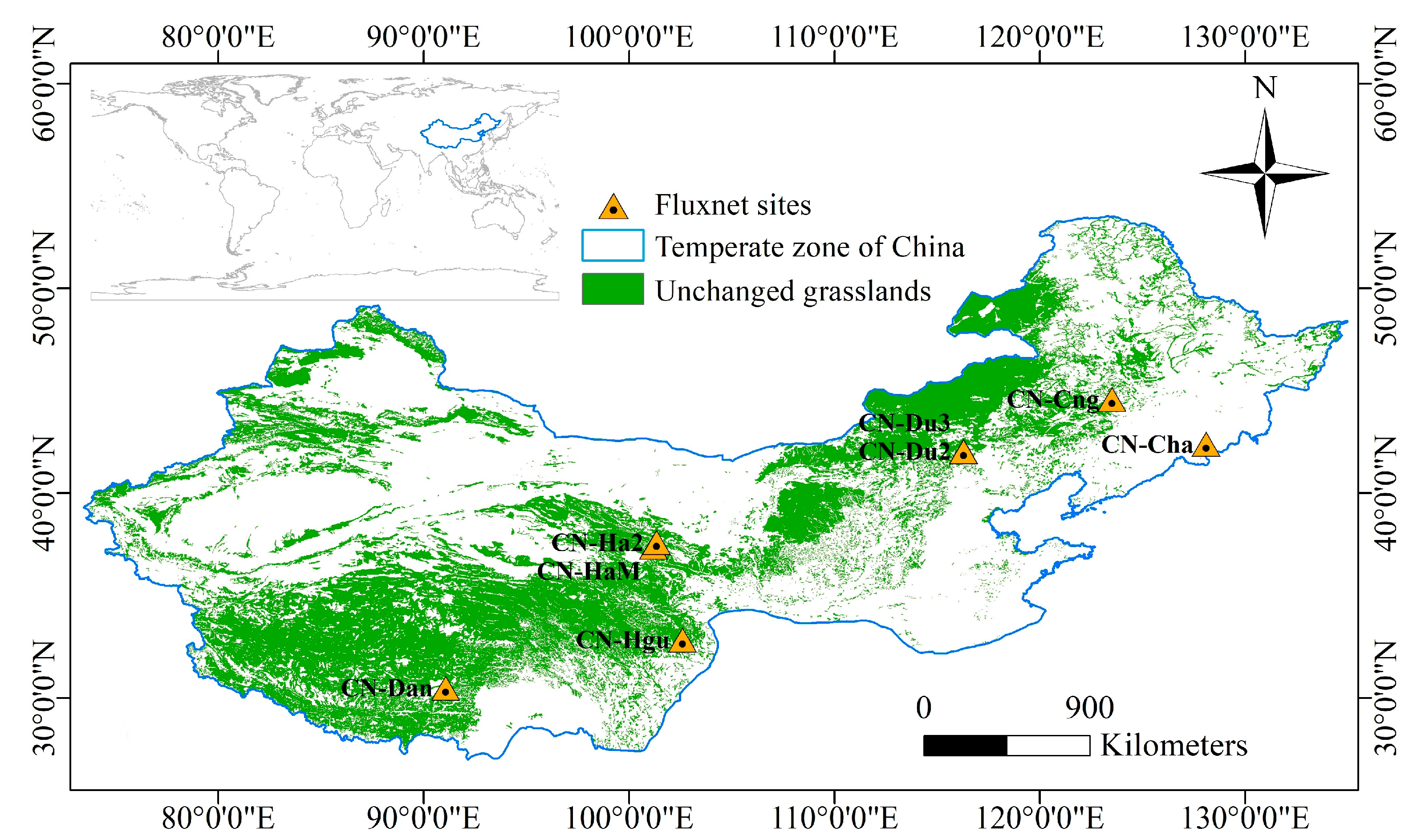
2.1. Study Area

The study area is roughly between 30° N and 50° N in the temperate zone in China (Figure 1), with annual mean temperature ranging from approximately −10 to 15 °C. Based on annual precipitation levels, the study area is divided into three categories: arid (<200 mm), semi-arid (200–400 mm), and semi-humid (400–800 mm) [24]. Seasons are distinctive in the area. Satellite measurements of the normalized difference vegetation index (NDVI) from low to high latitudes are less affected by solar zenith angles [25,26,27]. The research area for this study was limited to grasslands, excluding arable land, water bodies, man-made surfaces, and bare land. The area was determined by selecting pixels that have been consistently classified as grassland over the past two decades [19].

2.2. Data Sources and Pre-Processing

FLUXNET data were used as site data to verify the accuracy of extracting remote-sensing phenological data based on the normalized difference vegetation index (NDVI). The daily gross primary production (GPP) was obtained from FLUXNET datasets (https://fluxnet.fluxdata.org, accessed on 10 October 2022). The FLUXNET data website has implemented rigorous quality control processes for GPP data, involving screening to exclude periods of low turbulence and employing consistent methods to fill gaps in the data [28,29]. Table 1 provides an inventory of the locations and corresponding years for the GPP data collection.
The 20-year (2001–2020) MOD13A2 NDVI product with a spatial resolution of 1000 m and a temporal interval of 16 days was used to calculate the phenological metrics [30,31]. The MOD13A2 data are a widely used tool for dynamic monitoring of and research on vegetation at different scales and fully considers the influence of high coverage, low viewing angle, cloud shadow, aerosol, and other factors. The American National Aeronautics and Space Administration provided the data (NASA) (https://ladsweb.modaps.eosdis.nasa.gov/, accessed on 10 September 2021).
The GlobeLand30 dataset (http://www.globeland30.org/home_en.html, accessed on 15 November 2021) was used to extract the grassland. TM5, ETM+, and OLI multi-spectral photos of the US Landsat satellite and multi-spectral images from the China Environmental Disaster Reduction Satellite (HJ-1) were among the 30 m multi-spectral images utilized in the production of the GlobeLand30 data [32]. This dataset was based on satellite imagery and ground survey data, covering all land areas worldwide except Antarctica, including 31 categories of land use/cover types such as forests, grasslands, farmland, cities, etc.
The China Qinghai-Tibet Plateau Science Data Center provided the gridded monthly temperature and precipitation data for the years 2001 to 2020. (https://data.tpdc.ac.cn/zh-hans/search_index/, accessed on 5 August 2022). The Delta spatial downscaling method was used in China to create this dataset, which has a spatial resolution of 1000 m [33,34,35]. The data came from the worldwide high-resolution climate dataset published by WorldClim and the global 0.5° climate dataset published by CRU.

2.3. Methods

2.3.1. Vegetation Phenology Extraction

The methods for extracting phenological parameters based on the NDVI mainly include the threshold method, median method, and maximum slope method. Generally, the dynamic threshold method selects 20% and 50% [18,36], but there is no consensus on the optimal remote-sensing phenological extraction method for specific regions. Therefore, this study selected the dynamic threshold method (threshold 20%, threshold 50%) and the maximum slope method to extract the phenological metrics (SOS, EOS) of temperate grasslands in China.
The ground carbon flux phenology indicator data extracted from FLUXNET flux sites in the study are utilized as ground truth values to validate the accuracy of remotely sensed phenological data extracted from Chinese temperate grasslands using the first derivative and dynamic threshold methods. The determination coefficient (R2) of the univariate linear regression between the carbon flux phenology indicators at the flux sites and the remotely sensed phenology is compared, aiming to select the most suitable remote sensing phenology model within the study area.
(1)
Dynamic threshold method
The MODIS-NDVI extraction of vegetation phenology excluded pixels having an annual average NDVI of less than 0.1. The NDVI dataset was then filtered using the Timesat program with the SavitzkyGolay filtering method. The time points that correspond to 20% or 50% of the difference between the maximum and minimum NDVI values throughout a year were designated as SOS and EOS using the dynamic threshold approach [18,36]. The NDVI threshold was calculated as follows:
N D V I r a t i o = N D V I N D V I m i n N D V I m a x N D V I m i n
where the NDVIratio is the fitted NDVI at a given day, and NDVImax and NDVImin are the maximum and minimum NDVI each year.
(2)
Calculating the maximum slope of a first-order derivative model
Using the Double Logistic (DL) function to reconstruct the original NDVI time series curve, the calculation method for the DL function is as follows:
y ( t ) = a + b 1 + e c t d b e f ( t g )
where y(t) is the NDVI value of t (day of year, DOY) on a certain day of the year.
The maximum slope method defines the date corresponding to the point where the fitting curve rises the fastest as the SOS, and the date corresponding to the point where the fitting curve decreases the fastest as the EOS, that is, the dates corresponding to the maximum and minimum values in the first derivative of the fitting curve are the SOS and EOS, respectively.

2.3.2. Vegetation Phenology Extraction from FLUXNET Products

FLUXNET GPP data were employed to validate the accuracy of phenol extraction based on the NDVI. For each pixel in the Fluxnet GPP datasets, a moving average filter was applied to smooth the GPP curve. Subsequently, the 15% of the maximum daily GPP in the smoothed GPP curve was identified as the dates for the SOS and EOS [8,10,35].

2.3.3. Statistical Analysis

Non-parametric TheilSen and MannKendall trend analysis were used for the trend and significance of phenological metrics (SOS and EOS) [37,38]. This trend analysis does not need the normality of the data series and can lessen the influence of data outliers. Positive and negative values in the results represent delay and advance, respectively. The results can be used to analyze the phenology’s temporal and spatial patterns.
To understand how phenological changes were related to climate, two forms of correlation analysis were employed to examine the relationship between phenology and seasonal climate factors (specifically, average temperature and total precipitation). Firstly, a basic multiple linear regression was executed to establish the link between phenology and seasonal climate factors. Phenology (SOS or EOS) was used as the dependent variable in multiple linear regression, and the seasonal climate variables (temperature and precipitation) were used as the independent variables. The following is the formula:
Y = a1X1 + a2X2 + … + anXn
where an is the regression slopes, Xn is the independent variable, and Y is the dependent variable. Regression slopes between the SOS of years (2001–2020) and corresponding spring (March–May) precipitation, spring temperature, last-winter (December of the previous year–February) precipitation, and last-winter temperature and between the EOS and corresponding autumn (September–November) precipitation, autumn temperature, summer (June–August) precipitation, and summer temperature [26]. To enhance the robustness of the results, we use the variance inflation factor (VIF) to test the collinearity between independent variables. The variance inflation factor (VIF) is a measure of the severity of multicollinearity in multiple linear regression models. It represents the ratio of the variance of the regression coefficient estimator to the variance when assuming non-linear correlation between independent variables. Generally speaking, if the coefficient of variance inflation is less than 10, it indicates that there is no collinearity problem between the independent variables. The calculation formula is as follows:
V I F = 1 1 R i 2
where R i 2 is the multiple decision coefficient for the independent variable to perform multiple regression on the other independent variables.
The association between phenology (SOS or EOS) and seasonal climate variables was then investigated using partial correlation analysis, which removed the impact of other variables and identified the correlation between two variables.

3. Results

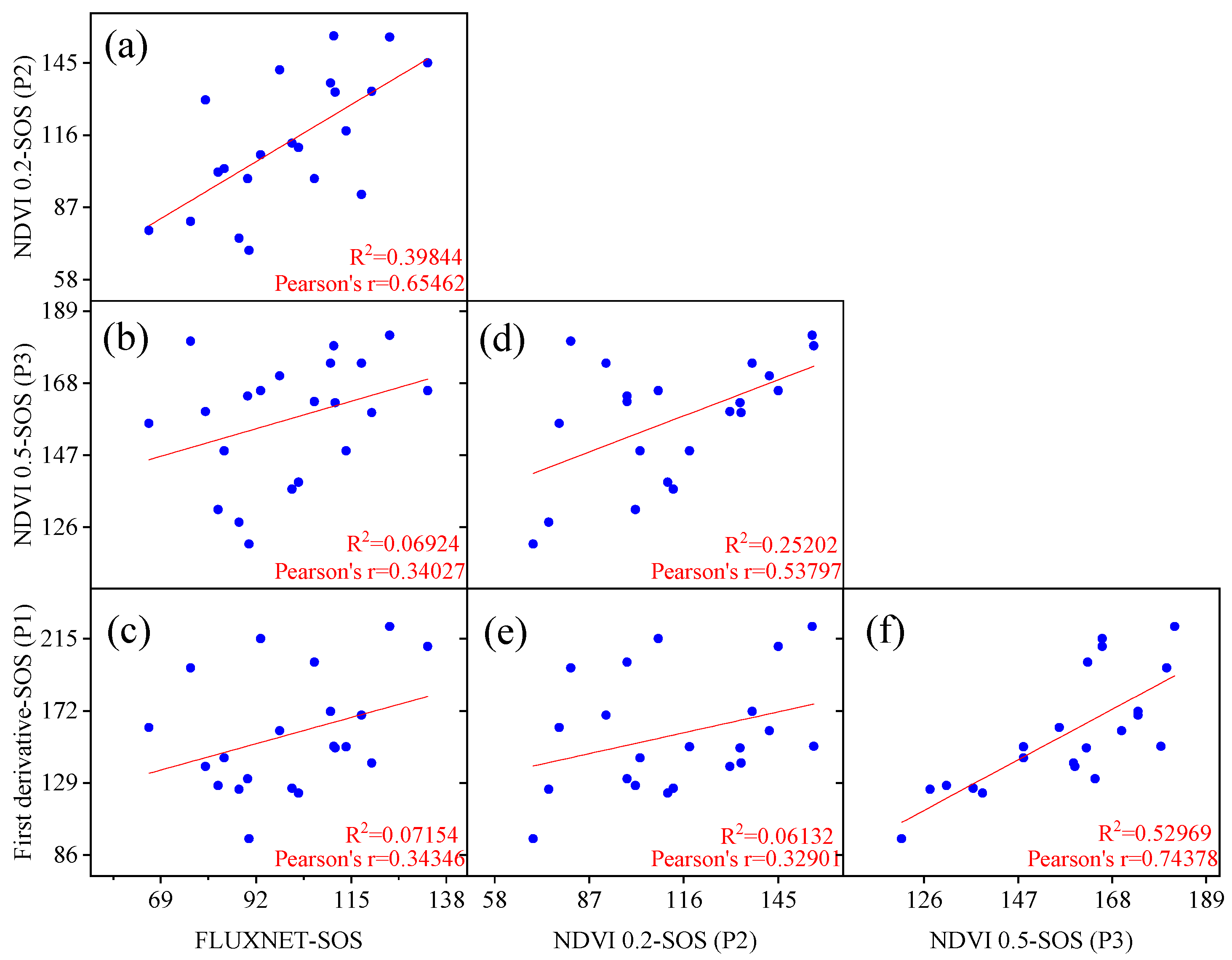
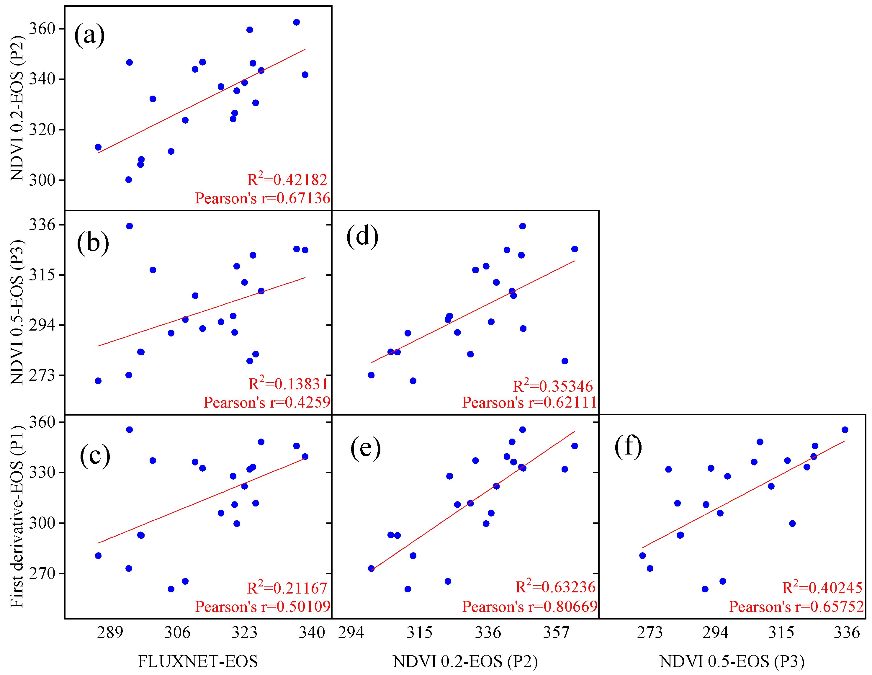
3.1. Evaluation of Vegetation Phenology Extracted from Satellite and Site Data

The linear regression results for the flux start of the growing season (SOS) and remote sensing SOS corresponding locations and years are shown in Figure 2. It was observed that the fitting performance of the remote sensing SOS extracted by models P1 (first derivative model) and P3 (dynamic threshold 50%) was poor, with R2 values of 0.072 and 0.069, respectively, much lower than the fitting results of the model P2 (dynamic threshold 20%) SOS with flux SOS (R2 = 0.398). Additionally, the study revealed that the P2 model was closer to the flux SOS values compared to the SOS values extracted by the P1 and P3 models. Both the P2 and P3 models employed the same method (dynamic threshold method) but with different thresholds. This indicates that the widely used 20% threshold in temperate regions is also suitable for Chinese temperate grasslands, while the 50% threshold is relatively high for Chinese temperate grasslands. Therefore, using the dynamic threshold method (20%) for extracting the remote sensing SOS data in the study will yield more reliable results.
The linear regression results for the flux end of the growing season (EOS) and remote sensing EOS corresponding locations and years are depicted in Figure 3. It was observed that the fitting performance of the remote sensing EOS extracted by models P1 and P3 was poor, with R2 values of 0.212 and 0.138, respectively, much lower than the fitting results of the model P2 EOS with the flux EOS (R2 = 0.422). Additionally, the study revealed that the P1 and P3 models were relatively closer to the flux EOS values compared to the P2 model. Despite the numerically larger EOS values extracted by the P2 model, the higher R2 value in the linear regression indicates the widespread applicability of the 20% threshold in Chinese temperate grasslands. The numerical difference does not affect the overall trend and variation of phenology, so the study adopted the dynamic threshold method (20%) for extracting remote sensing EOS data.

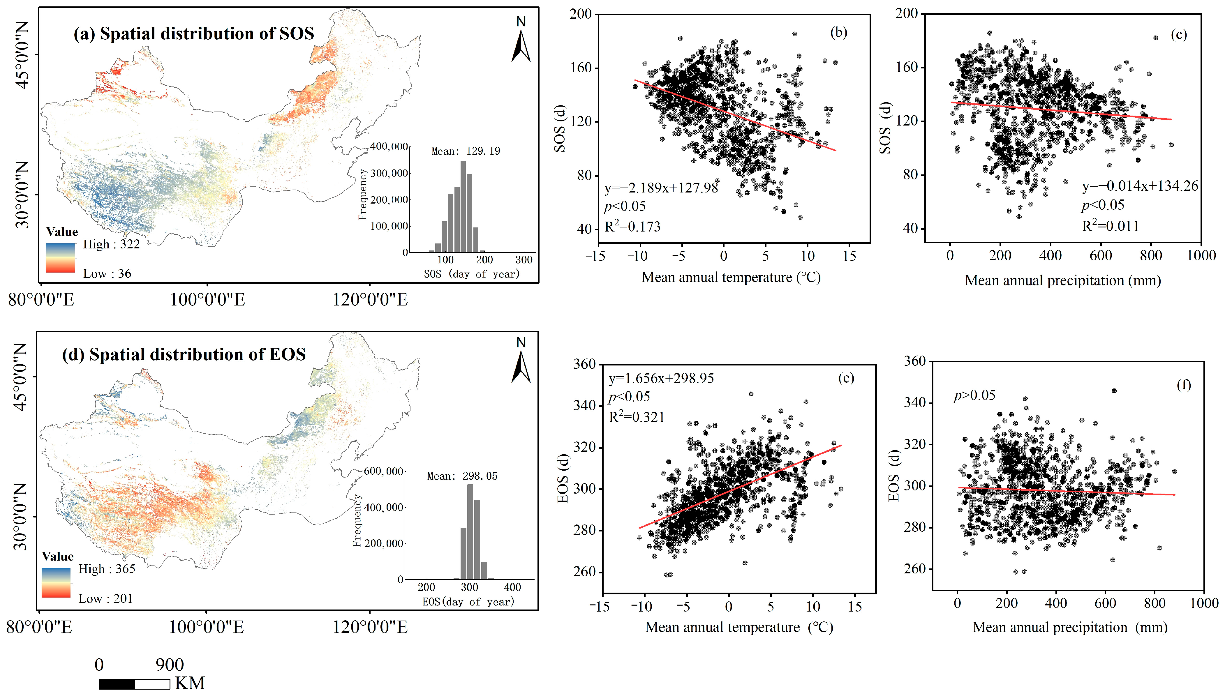
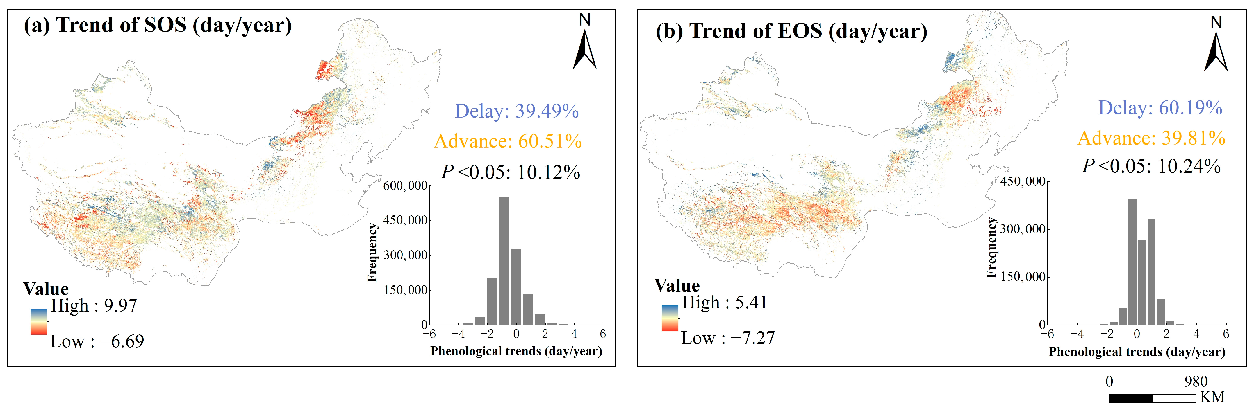
3.2. The Spatiotemporal Changes in Vegetation Phenology

The spatial pattern of multi-year (2001–2020) averages of phenological metrics (SOS, EOS) of temperate grassland in China are depicted in Figure 4. More than 89.5% of the pixels of the SOS occurred between early April (day 100) and early May (day 160) (Figure 4a). More than 91.3% of the pixels of the EOS occurred between early October (day 285) and early November (day 310) (Figure 4d). At the regional scale, as the mean annual temperature increases by 1 °C, the SOS advances by 2.2 days (Figure 4b) and the EOS is delayed by 1.7 days (Figure 4c), and as the mean annual precipitation increases by 100 mm, the SOS advances by 1.4 days (Figure 4c).
Over the past 20 years, 60.5% of the pixels of the SOS showed advance and 39.5% showed delay. Among the EOS, 39.8% of the pixels show advance, and 60.2% of the pixels show delay (Figure 5). Although most pixels showed early SOS and delayed EOS between 2001 and 2020, the study found that over 89% of regions did not show significant long-term trends in SOS and EOS (p > 0.05) (Figure 5).

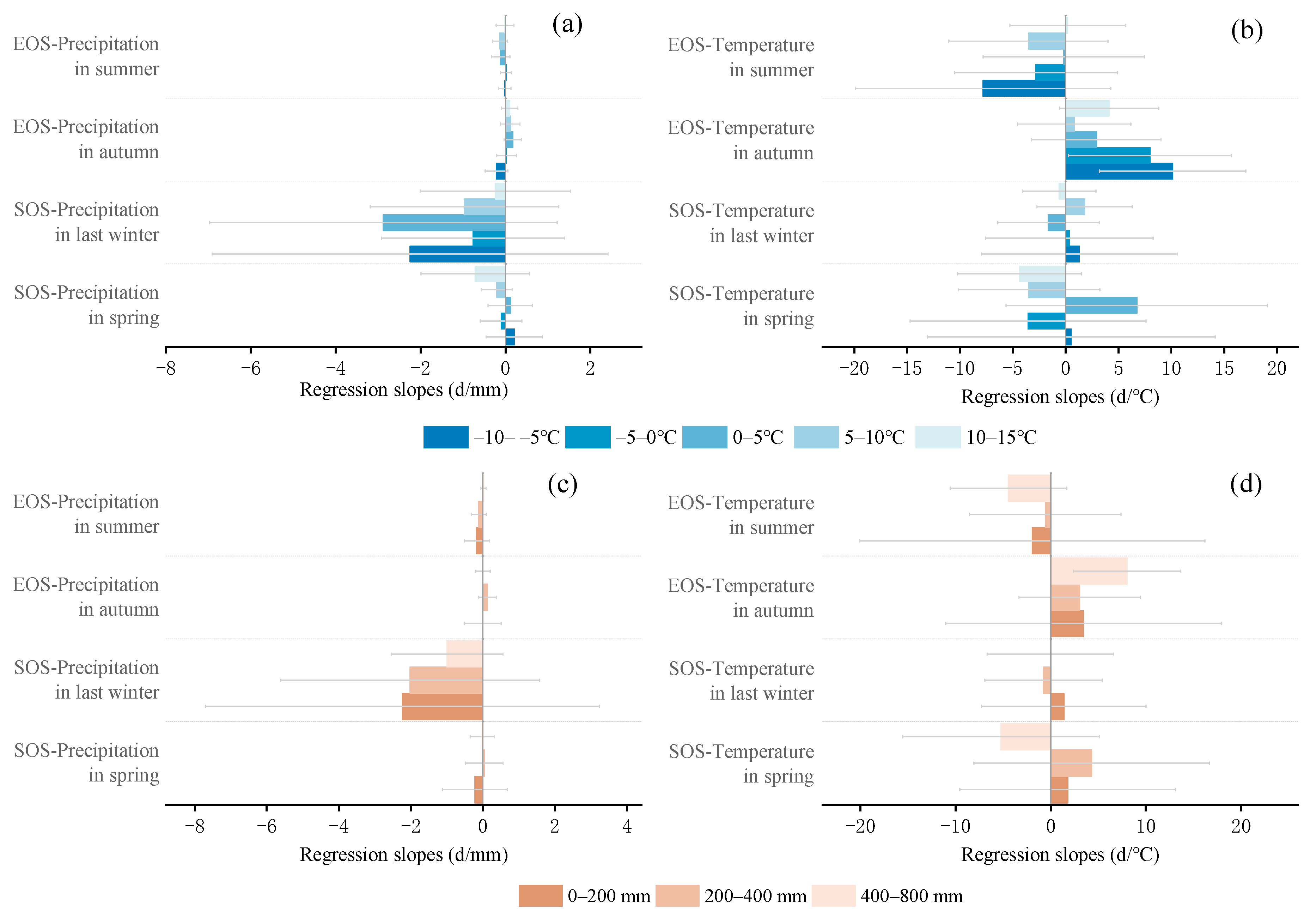
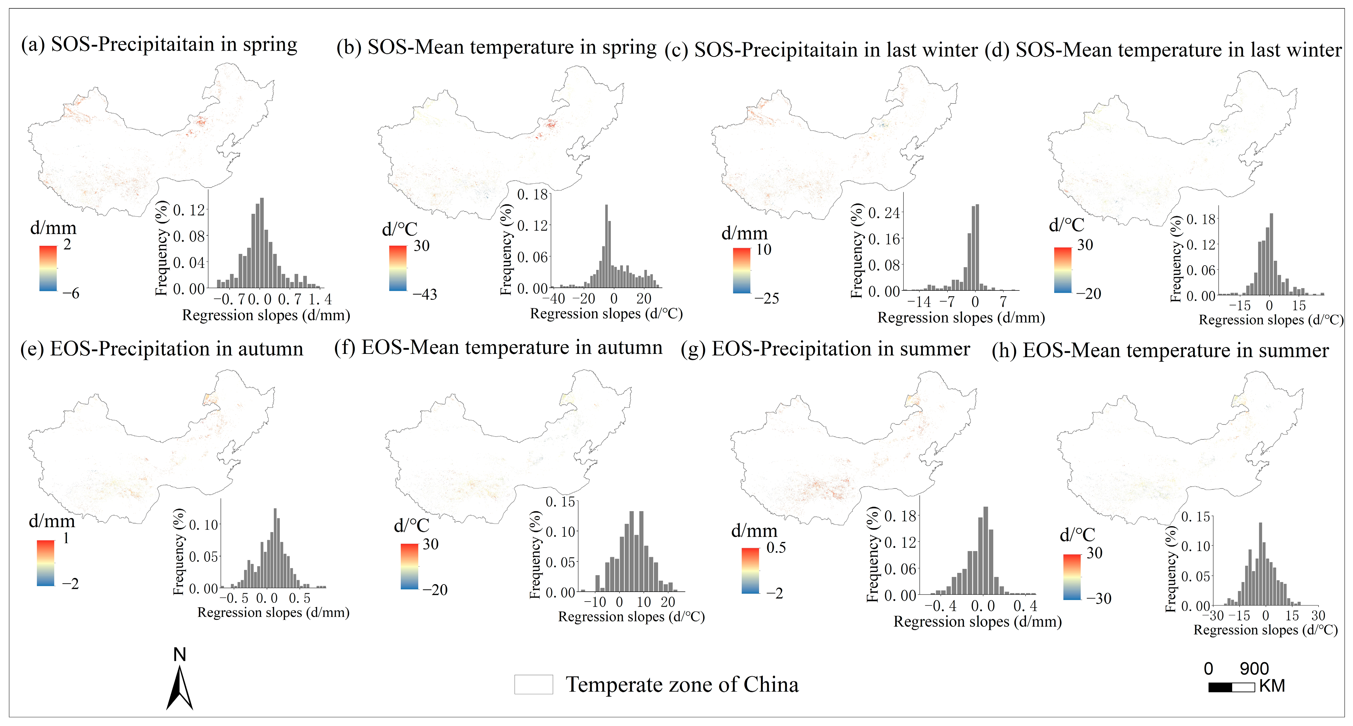
3.3. Sensitivity of Phenology to Seasonal Climate from 2001 to 2020 and Regional Differences

The multivariate regression analysis of phenological metrics vs. seasonal climate by pixel from 2001 to 2020 is shown in Figure 6, and the sensitivity of phenological metrics to seasonal climate changes with mean annual temperature and precipitation is represented by a scatter plot (Figure 7 and Figure 8). The variance inflation factor (VIF) between the independent variables of seasonal climate is all less than 10, indicating that there is no collinearity between the independent variables (Figures S1–S3). The sensitivity of the SOS to spring temperature and last-winter precipitation varied spatially and linearly with the increase in mean annual precipitation (p < 0.05) (Figure 8b,c), rather than mean annual temperature (Figure 7a–d). Furthermore, the sensitivity of the EOS to summer and autumn climate was influenced by both mean annual temperature and precipitation (Figure 7e,f and Figure 8e,f). The last-winter precipitation had a greater impact on the SOS than spring precipitation did (Figure 9a), with the largest contribution of −2.23 d/mm in regions with precipitation ranging from 0 to 200 mm. Autumn temperature impacted the EOS most, with the highest contribution of 10.13 d/°C in regions with temperatures ranging from −10 to −5 °C (Figure 9b).

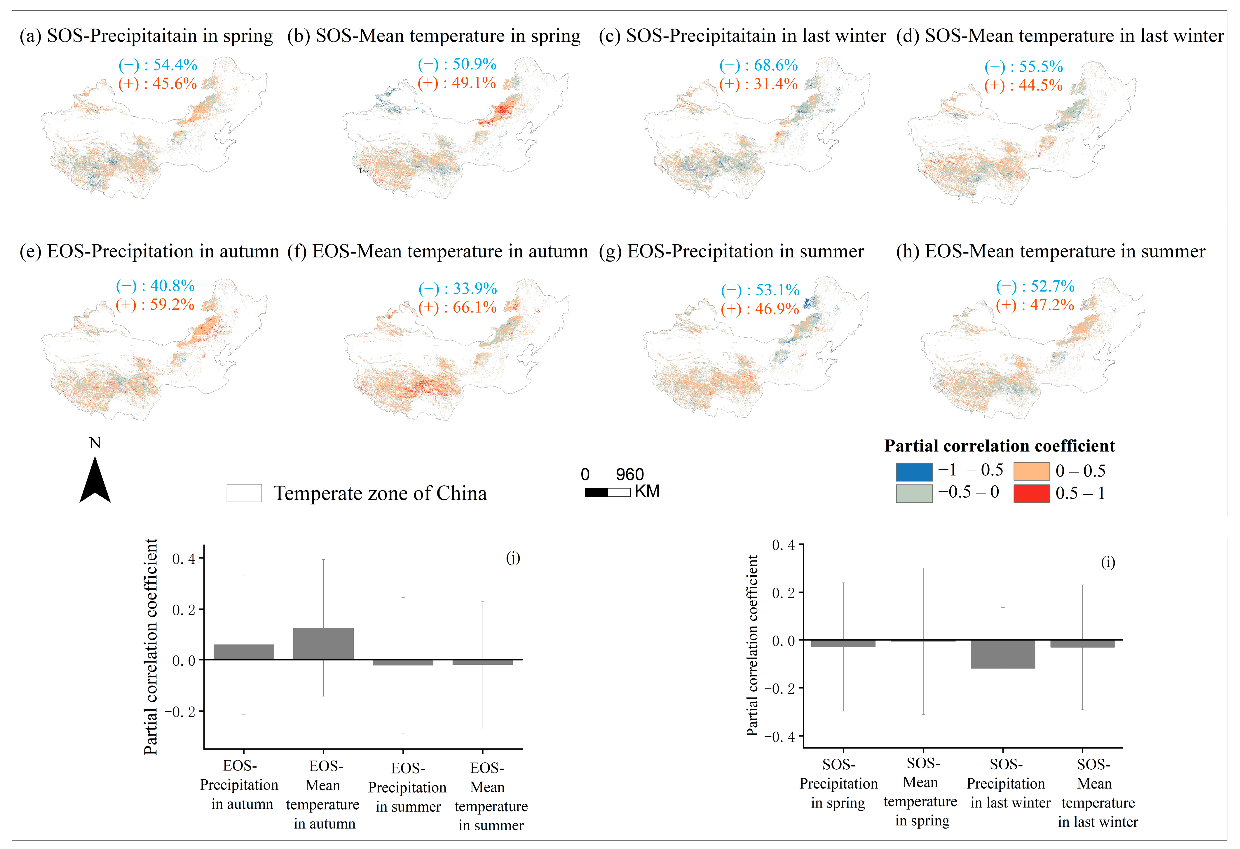
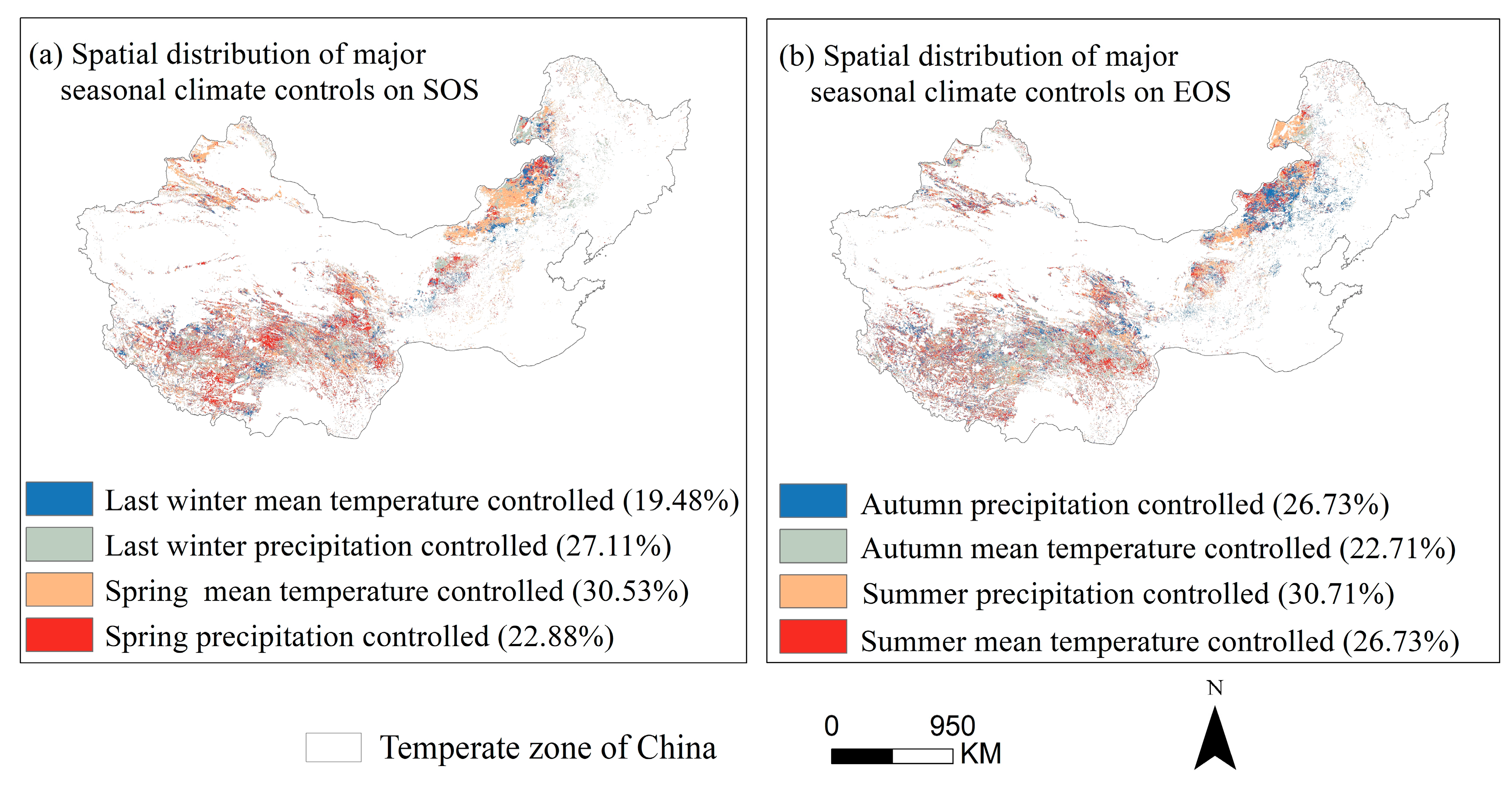
3.4. Partial Correlation Analysis to Determine the Area Division of Relative Importance

Through partial correlation analysis of phenology and seasonal climate from 2001 to 2020 pixel by pixel. We discovered that the response of phenology to seasonal climate varied spatially (Figure 10), with the strongest partial correlation coefficient between last-winter precipitation and the SOS (Figure 10i). Last-winter precipitation had a negative impact on SOS for a larger number of pixels (68.6%) (Figure 10c,i). Similarly, the autumn temperature had a positive impact on the EOS for a larger number of pixels (66.1%) (Figure 10f,j). We created a controlling-factor map based on the greatest partial correlation coefficient between phenology and seasonal climatic variables (temperature and precipitation) to determine the regions where changes in phenology were mostly controlled by either temperature or precipitation (Figure 11). In more than 30% of the pixels analyzed, the analysis revealed that spring temperature was the main cause of interannual change in the SOS (Figure 11a), which was more prevalent in Inner Mongolia’s center and eastern regions. In contrast, summer precipitation was the primary controlling factor for interannual variation in the EOS in more than 30% of the pixels examined, with these areas mainly located in the Hulunbuir (Figure 11b).

4. Discussion

4.1. Spatial Heterogeneity of Phenology Trend

In this study, large spatial variability in phenology was found in temperate grassland in China (Figure 4). The SOS in temperate regions of China mainly occur between the 100th and 160th days, which is consistent with the SOS observed in China from 2001 to 2014 [39]. The SOS in the Loess Plateau and the eastern part of the Qinghai-Tibet Plateau occurs later. We speculate that this delay may be attributed to the geographical location of the Loess Plateau, situated in the northwest inland of China and influenced by the northwest monsoon, resulting in less precipitation and a drier climate. In the Qinghai-Tibet Plateau, the SOS of grasslands around the Gangdise Mountains occurs between the 170th and 180th day. Early EOS is predominantly observed in the northeast and northwest regions of temperate grasslands, whereas alpine grasslands exhibit earlier EOS dates compared to other grasslands. Conversely, late EOS is mainly distributed in the central and eastern regions of Inner Mongolia [40].
We found that higher temperature regions had earlier start and later end dates for the growing season (Figure 4b,c), and earlier SOS in relatively humid regions (Figure 4c). The phenological metrics trends were heterogeneous in both direction and magnitude at the regional scale across the study period (Figure 5), suggesting that plant phenology under different hydrothermal regions responded diversely to changes in a unit change in temperature and precipitation. The SOS advance and EOS delay have been found in previous studies [41,42,43]. However, with the extension of the research cycle, the SOS shows a slow development trend. For example, Jeong et al.’s study on temperate regions of the Northern Hemisphere showed that during the 1982–1999 study period, the progress rate of the SOS was 0.29 days per year, but then the progress of the SOS slowed down, slowing down at a rate of 0.02–1 days per year in the later stages (2000–2008) [43]. In addition, Zhao et al. revealed that from 1982 to 2013, the average SOS in Northeast China did not show a significant upward trend (0.04 days per year) [44]. Some studies believe that the spatial heterogeneity of phenological trends was caused by the different responses of vegetation in the biological community to the climate in different seasons [45]. Over the past 20 years, 60.5% of the pixels in the SOS showed advance and 39.5% showed delay. Among the EOS, 39.8% of the pixels show advance, and 60.2% of the pixels show delay (Figure 5). Although most pixels showed early SOS and delayed EOS between 2001 and 2020, the study found that over 89% of regions did not show significant long-term trends in the SOS and EOS (Figure 5). This is consistent with previous research results, and there was no significant trend in phenology in some study areas. For example, the warming of forests in the Northeastern United States did not have a significant impact on phenology [46]. In the study of the global scale, Central Asia and the Qinghai-Tibet Plateau, SOS, and EOS trends were not significant [18,47,48]. Additionally, CentralWest Asian grasslands showed a forward shift in all SOS pixels, whereas no such notable trend was seen for North American grasslands or East Asian grasslands [49]. There are studies suggesting that phenology reacts differently or even in the opposite way to various seasonal climates [16,22,50]. Through studying the interannual trends of monthly climate, we found that from 2001 to 2020, the trends of temperature and precipitation were not significant, and even the trends were opposite in different months (Figure S4a,b). The interactive effects of seasonal climate on phenology are caused by climate change, which slows down the long-term trend of phenology. Some studies also suggest that the uncertainty of this phenological trend is often attributed to the different phenological changes of different vegetation types, and the complexity of regional climate leads to differences in the response of vegetation phenology to climate [51]. Previous studies have found that differences in the response of different species phenology to climate change can lead to unsynchronized ecological interactions, thereby threatening ecosystem functions [39,52]. In other words, key seasonal interactions between species can become unsynchronized over time, affecting the duration of inter species interactions, crop production, and pollination seasons, potentially resulting in serious consequences for wild populations and ecosystem functions [36]. Therefore, the uncertainty of long-term phenological trends and the increase in interannual variability will inevitably lead to the exacerbation of this serious consequence.

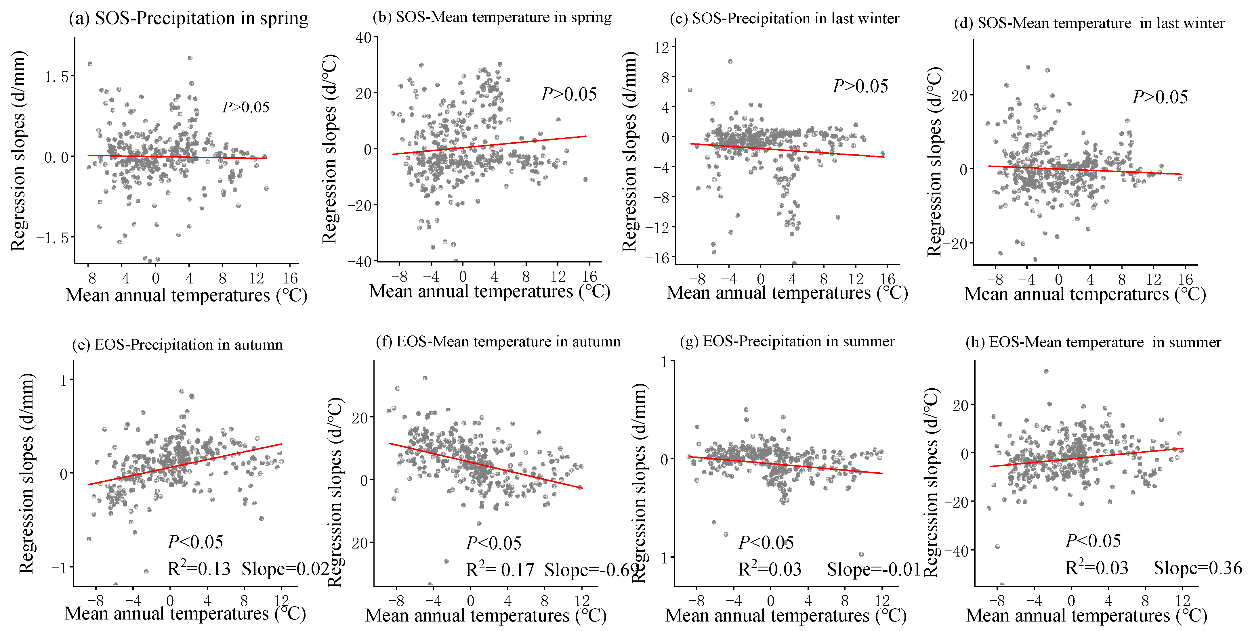
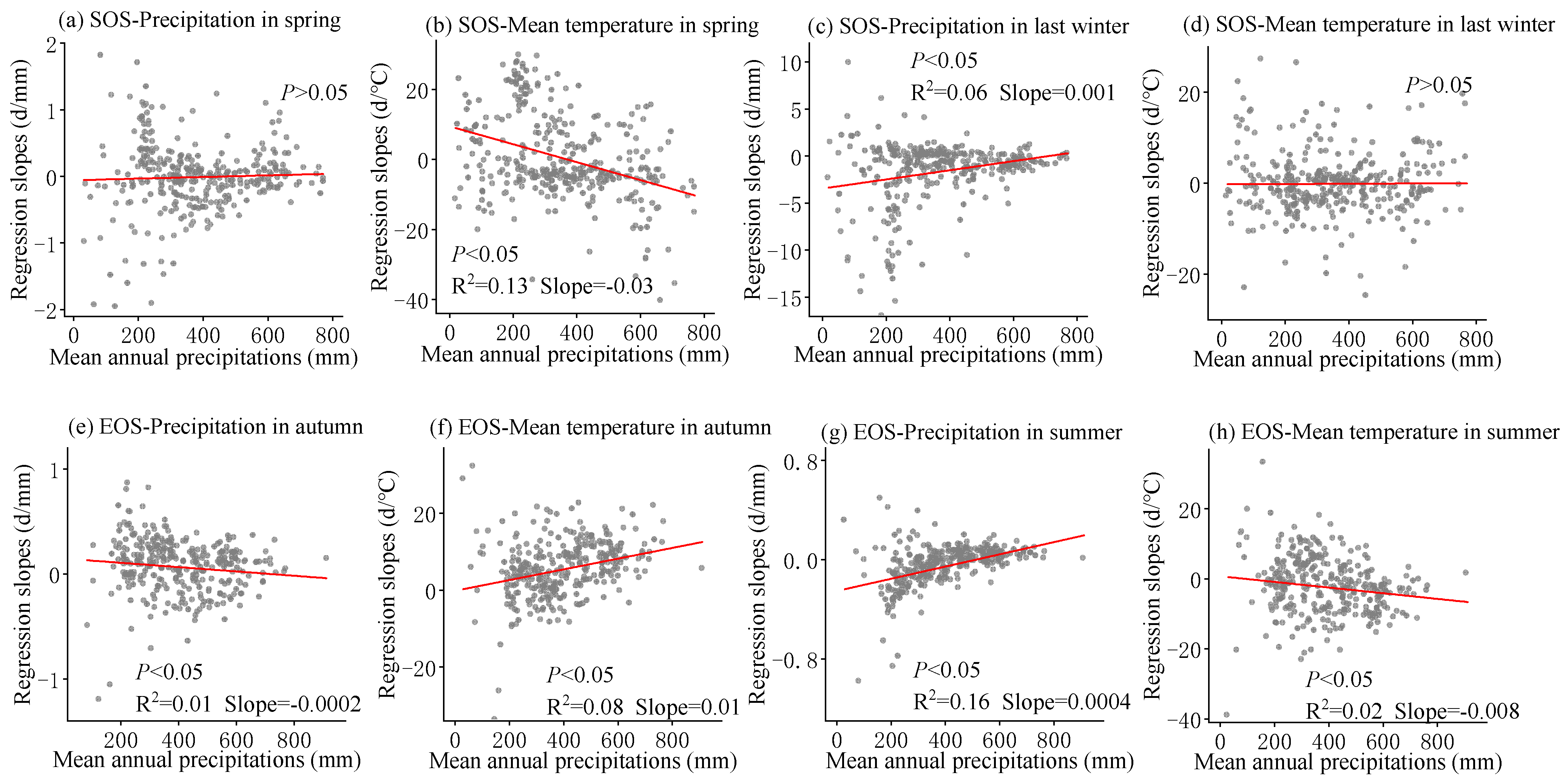
4.2. The Sensitivity of SOS to Seasonal Climate Was Regulated by Regional Climate from 2001 to 2020

The warm temperatures in spring will accelerate the accumulation of heat, promoting the resumption of active growth [53]. Previous studies have indicated that the increase in winter temperatures may result in insufficient cold accumulated temperature requirements for vegetation, weakening the process of breaking dormancy and consequently leading to a later start of the growing season (SOS) [54]. Earlier research in the Qinghai-Tibet Plateau region suggested that, despite the advancement of the growing season due to warm springs, the warm conditions in winter could cause a delay in the spring phase [36]. However, this study observed that a warm winter could also lead to an earlier spring phase, and these disparate results may be attributed to regional conditions or species differences. The lag effects of seasonal climate on the phenological responses of different vegetation vary, and the extent of cold requirement differs [26]. While climate warming tends to advance the SOS, the interactive effects of seasonal climate on phenology introduce uncertainties in the long-term trend of the SOS. Prolonged warming may reinforce these impacts, potentially weakening or even reversing the long-term trend of the SOS [55]. Plants in humid regions of China and plants in regions with higher mean annual temperatures may be more sensitive to temperature [25,56]. These outcomes support our findings that between 2001 and 2020, the SOS was more responsive to spring temperature in humid regions (Figure 8b and Figure 9d). In addition, our research results reveal that the sensitivity of the SOS to spring temperature varies linearly from positive to negative with the increase in annual average precipitation (p < 0.05) (Figure 8b), indicating that an increase in spring temperature in relatively humid areas is more conducive to early SOS, while an increase in spring temperature in relatively arid areas leads to delayed SOS [25]. Previous studies have also found that temperature sensitivity is higher in humid areas of China [14,15], and the positive correlation in arid areas may be related to the impact of spring water stress on plant growth. Limited water potential can inhibit plant growth and photosynthetic activity, while the increase in spring temperature leads to rapid evaporation of water in arid areas [57]. Strengthening water stress leads to decreased vegetation activity and delayed phenology [57]. Therefore, an increase in pre-season precipitation can alleviate water stress and lead to earlier spring phenology. In addition, the precipitation in the winter of the previous year was negatively correlated with the SOS, and the increase in precipitation in the winter of the previous year led to an advance in the SOS (Figure 10c). Compared with semi-humid and semi-arid regions, the SOS in arid regions is more sensitive to precipitation in the last winter (Figure 8c). Previous studies have also found that in typical grasslands and desert grasslands in Inner Mongolia, the rapid decrease in available water delayed the occurrence of the SOS, while seasonal drought significantly suppressed the SOS in grasslands [58], especially in typical grasslands [59]. In the Hulunbuir Plateau region, there is a significant negative correlation between the SOS and total spring precipitation, indicating that spring precipitation controls vegetation growth, especially in semi-arid areas [57]. Our research indicates that temperature and precipitation both contributed to the SOS of temperate grasslands in China [60,61], but the sensitivity of the SOS to spring temperature and last-winter precipitation during 2001–2020 was mainly controlled by mean annual precipitation rather than temperature (Figure 8b,c).

4.3. The Sensitivity of EOS to Seasonal Climate Was Regulated by Regional Climate from 2001 to 2020

Autumn temperatures showed a consistent controlling function in regulating EOS variations from 2001 to 2020 for the majority of pixels (Figure 9b and Figure 10j), which was consistent with previous research. Increasing autumn temperatures reduced frost risk and delayed the EOS due to insufficient cold accumulation [59]. Interestingly, increasing summer temperatures advanced the EOS during the study period (Figure 9b,d). Previous studies have suggested that the increase in summer temperature and physiological activity may promote early autumn senescence through various possible mechanisms, including developmental and nutritional limitations, seasonal accumulation of water stress, and radiation induced leaf senescence [49,62]. On the contrary, the rapid decrease in autumn temperature will directly lead to early autumn aging [10]. However, our study showed the opposite, that increasing summer precipitation also advanced the EOS (Figure 8g and Figure 9a,c), and the sensitivity was stronger in warmer areas (Figure 7g). One possible reason for this is the differences in regional climate and study subjects, leading to variations in the response of the EOS to summer temperatures [63]. Another possible explanation is that high summer temperatures in relatively humid areas can enhance vegetation growth by affecting vegetation carboxylation and enhancing vegetation photosynthesis, completing the entire growing season in advance [64]. Previous studies on deciduous trees in Europe have shown a negative feedback between growth season productivity and autumn phenology, with increased productivity leading to earlier aging [65]. Early season warming leads to early leaf growth and accelerated tissue maturation in spring, often leading to earlier EOS dates [66]. Similarly, it has been found through experimental and long-term observational studies that the improvement in productivity during spring and summer due to the increase in carbon dioxide, temperature, or light levels can lead to premature leaf aging [65]. We also observed similar phenomena in our study results, such as summer temperature and precipitation having a more negative correlation with the EOS (Figure 10j). In addition, the sensitivity of the EOS to summer precipitation was more sensitive in warm regions (Figure 7g), and the sensitivity to summer temperature was more sensitive in relatively humid regions (Figure 8h and Figure 9d). This has also been found in previous studies, which suggest that the increase in the EOS observed during temperature rise and growth before the summer solstice may be related to the availability of soil resources throughout the growing season [67]. The optimal growth conditions in spring (high temperature and sufficient precipitation) may deplete the nitrogen availability of trees, leading to early spring and early leaf senescence [68]. Therefore, for areas with good water and thermal conditions, the reduction in soil moisture in autumn due to summer warming is not the main reason for advancing autumn phenology. The growth limitation of plants is an important biological factor for advancing autumn phenology [19]. In addition, with the increase in atmospheric CO2 concentration, the C:N ratio of leaves increases, leading to microbial immobilization and reduced nitrogen accessibility, which may also be important reasons for early leaf senescence [69]. The sensitivity of the EOS to seasonal climate showed a linear relationship from 2001 to 2020 with mean annual precipitation and temperature changes (Figure 7e–h and Figure 8e–h). These results also suggested that autumn phenology was influenced by both the early growth of plants and environmental factors, making it more susceptible to disturbances caused by climate. The improved model for plant development and growth under climate change needs to incorporate the composite effects of seasonal warming on phenology.

4.4. Uncertainty and Outlook

The MODIS-NDVI data have been widely used for phenological monitoring. we employed multiple datasets (FLUXNET-GPP, and MODIS-NDVI) for cross-validation and to obtain a better evaluation of vegetation phenological dynamics. Our results show that phenological metrics exhibit a good fit in linear regression analysis; although the results have consistency between phenological information extracted using the MODIS-NDVI and other datasets, they also have some flaws (Figure 2 and Figure 3). Seasonal temperature and precipitation are important controlling factors of vegetation phenology. Nevertheless, the properties of the topography and the soil, as well as radiation, have an impact on the spatiotemporal patterns of phenology. Due to the difficulty of accounting for all these factors in large-scale remote sensing applications, a more comprehensive understanding of vegetation phenology shifts requires further investigation, particularly against the background of global climate change. Leveraging the advantages of wide-ranging remote sensing data, long time series, and numerous samples (pixels), we have explained the response of phenology to seasonal temperature and precipitation and its relationship with regional climate, thereby providing novel insights into predicting phenological changes in different regions resulting from climate warming. The NDVI is influenced by light reflection, while SIF (Sun-Induced Fluorescence) is derived from the fluorescence emission of vegetation itself, making it more sensitive to non-photosynthetic changes and providing more accurate vegetation phenological information. SIF has a greater sensitivity and dynamic range than the NDVI, and can capture small changes in vegetation physiological status and a wider dynamic range. For example, recent research on using SIF remote sensing for phenological monitoring may improve the monitoring of grassland photosynthetic phenols [70,71,72].

5. Conclusions

In this study, we investigated the impact and sensitivity of seasonal climate on phenology (SOS and EOS) in the temperate grasslands of China from 2001 to 2020. Our results indicated that based on trend analysis of vegetation phenology on a pixel-by-pixel basis, more than 89% of pixels had no significant trend from 2001 to 2020. The sensitivity of the SOS to late-winter precipitation and spring temperatures throughout the study period showed a linear variation with the rise in mean annual precipitation rather than shifting in response to the increase in mean annual temperature. Last-winter precipitation increases promoted an advance in the SOS and had a greater impact on the SOS than spring precipitation did, with the SOS advancing up to 2.23 days for every 1 mm increase in the last-winter precipitation. The EOS was sensitive to autumn temperature, being delayed 10.13 days for every 1 °C increase in autumn temperature in regions with temperatures between −10 °C and −5 °C. Compared to the SOS, the EOS may be influenced by both early plant growth and environmental factors, making its response to future climate change more uncertain. The increasing last-winter precipitation led to an advance in the SOS, and increasing in autumn temperatures led to a delay in the EOS in most areas of the temperate grassland in China during the study period. Our research has significant ramifications for anticipating regional phenology shifts in climate change with rising temperatures and unpredictable precipitation. In addition, our study offers new perspectives on how phenology affects climate sensitivity in the context of future climate change.

Supplementary Materials

The following supporting information can be downloaded at: https://www.mdpi.com/article/10.3390/land13030399/s1, Figure S1: The variance inflation factors (VIF) of spring temperature (a), spring precipitation (b), temperature of the last winter (c), and precipitation of the last winter (d) with respect to the other three variables respectively; Figure S2: The variance inflation factors (VIF) of autumn temperature (a), autumn precipitation (b), summer temperature (c), and summer precipitation (d) with respect to the other three variables respectively; Figure S3: The pixel statistics of the variance inflation factors (VIF) for raster data, with the x-axis representing autumn rainfall (Au-pre), autumn temperature (Au-temp), spring rainfall (Sp-pre), spring temperature (Sp-temp), summer rainfall (Su-pre), summer temperature (Su-temp), previous year’s winter rainfall (Win-pre), and previous year’s winter temperature (Win-temp) in sequence; Figure S4: The interannual changes in monthly mean temperature (a) and mean precipitation (b) in temperate zone of China. Line chart show the annual monthly climate attributes, the numbers in orange font and blue font indicate the slope of linear regression fitting and the coefficient of variation (cv) from 2001 to 2020, respectively.

Author Contributions

All authors made intellectual contributions to this research work. X.W.: Writing—original draft. M.X.: Writing—original draft. H.Z.: Writing—original draft. X.L. (Xinyue Liu): Writing—original draft. Z.G.: Writing—original draft. X.L. (Xinhao Li): Writing—original draft. T.Z.: Writing—review and editing. Together, all authors discussed and interpreted the results. All authors have read and agreed to the published version of the manuscript.

Funding

This work was supported by the National Key Research and Development Program of China [2020YFA0608100], Beijing Ecological Observatory Network [GJH-2023-027] and the National Natural Science Foundation of China [NSFC: 32071842, 32071843, 32101588, 31901366].

Data Availability Statement

The original contributions presented in the study are included in the article/Supplementary Materials, further inquiries can be directed to the corresponding author.

Conflicts of Interest

Author M.X. was employed by the Observation and Research Station of Ecological Restoration for Chongqing Typical Mining Areas. He participated in the writing of this study. The role of the company is to participate in writing. The remaining authors declare that the study was conducted in the absence of any commercial or financial relationships that could be interpreted as potential conflicts of interest.

References

  1. Piao, S.; Ciais, P.; Friedlingstein, P.; Peylin, P.; Reichstein, M.; Luyssaert, S.; Margolis, H.; Fang, J.; Barr, A.; Chen, A.; et al. Net carbon dioxide losses of northern ecosystems in response to autumn warming. Nature 2008, 451, 49–52. [Google Scholar] [CrossRef]
  2. Richardson, A.D.; Anderson, R.S.; Arain, M.A.; Barr, A.G.; Bohrer, G.; Chen, G.; Chen, J.M.; Ciais, P.; Davis, K.J.; Desai, A.R.; et al. Terrestrial biosphere models need better representation of vegetation phenology: Results from the North American Carbon Program Site Synthesis. Glob. Chang. Biol. 2012, 18, 566–584. [Google Scholar] [CrossRef]
  3. Piao, S.; Liu, Q.; Chen, A.; Janssens, I.A.; Fu, Y.; Dai, J.; Liu, L.; Lian, X.; Shen, M.; Zhu, X. Plant phenology and global climate change: Current progresses and challenges. Glob. Chang. Biol. 2019, 25, 1922–1940. [Google Scholar] [CrossRef] [PubMed]
  4. Wang, L.; De Boeck, H.J.; Chen, L.; Song, C.; Chen, Z.; McNulty, S.; Zhang, Z. Urban warming increases the temperature sensitivity of spring vegetation phenology at 292 cities across China. Sci. Total. Environ. 2022, 834, 155154. [Google Scholar] [CrossRef] [PubMed]
  5. Meng, L.; Mao, J.; Zhou, Y.; Richardson, A.D.; Lee, X.; Thornton, P.E.; Ricciuto, D.M.; Li, X.; Dai, Y.; Shi, X.; et al. Urban warming advances spring phenology but reduces the response of phenology to temperature in the conterminous United States. Proc. Natl. Acad. Sci. USA 2020, 117, 4228–4233. [Google Scholar] [CrossRef]
  6. Prevey, J.; Vellend, M.; Ruger, N.; Hollister, R.D.; Bjorkman, A.D.; Myers-Smith, I.H.; Elmendorf, S.C.; Clark, K.; Cooper, E.J.; Elberling, B.; et al. Greater temperature sensitivity of plant phenology at colder sites: Implications for convergence across northern latitudes. Glob. Chang. Biol. 2017, 23, 2660–2671. [Google Scholar] [CrossRef] [PubMed]
  7. Diez, J.M.; Ibanez, I.; Miller-Rushing, A.J.; Mazer, S.J.; Crimmins, T.M.; Crimmins, M.A.; Bertelsen, C.D.; Inouye, D.W. Forecasting phenology: From species variability to community patterns. Ecol. Lett. 2012, 15, 545–553. [Google Scholar] [CrossRef] [PubMed]
  8. Richardson, A.D.; Black, T.A.; Ciais, P.; Delbart, N.; Friedl, M.A.; Gobron, N.; Hollinger, D.Y.; Kutsch, W.L.; Longdoz, B.; Luyssaert, S.; et al. Influence of spring and autumn phenological transitions on forest ecosystem productivity. Proc. Natl. Acad. Sci. USA 2010, 365, 3227–3246. [Google Scholar] [CrossRef]
  9. Cong, N.; Shen, M.G. Variation of satellite-based spring vegetation phenology and the relationship with climate in the Northern Hemisphere over 1982 to 2009. J. Appl. Ecol. 2016, 27, 2737–2746. [Google Scholar] [CrossRef]
  10. Wang, X.; Xiao, J.; Li, X.; Cheng, G.; Ma, M.; Zhu, G.; Arain, M.A.; Black, T.A.; Jassal, R.S. No trends in spring and autumn phenology during the global warming hiatus. Nat. Commun. 2019, 10, 2389. [Google Scholar] [CrossRef]
  11. Wang, G.; Luo, Z.; Huang, Y.; Xia, X.; Wei, Y.; Lin, X.; Sun, W. Preseason heat requirement and days of precipitation jointly regulate plant phenological variations in Inner Mongolian grassland. Agric. For. Meteorol. 2022, 314, 108783. [Google Scholar] [CrossRef]
  12. Wang, S.; Zhang, L.; Huang, C.; Qiao, N. An NDVI-Based Vegetation Phenology Is Improved to be More Consistent with Photosynthesis Dynamics through Applying a Light Use Efficiency Model over Boreal High-Latitude Forests. Remote Sens. 2017, 9, 695. [Google Scholar] [CrossRef]
  13. Doussoulin-Guzman, M.-A.; Perez-Porras, F.-J.; Trivino-Tarradas, P.; Rios-Mesa, A.-F.; Garcia-Ferrer Porras, A.; Mesas-Carrascosa, F.-J. Grassland Phenology Response to Climate Conditions in Biobio, Chile from 2001 to 2020. Remote Sens. 2022, 14, 475. [Google Scholar] [CrossRef]
  14. Post, E.; Steinman, B.A.; Mann, M.E. Acceleration of phenological advance and warming with latitude over the past century. Sci. Rep. 2018, 8, 3927. [Google Scholar] [CrossRef] [PubMed]
  15. Ren, S.; Chen, X.; Pan, C. Temperature-precipitation background affects spatial heterogeneity of spring phenology responses to climate change in northern grasslands (30 degrees N-55 degrees N). Agric. For. Meteorol. 2022, 315, 108816. [Google Scholar] [CrossRef]
  16. Wang, J.; Li, M.; Yu, C.; Fu, G. The Change in Environmental Variables Linked to Climate Change Has a Stronger Effect on Aboveground Net Primary Productivity Than Does Phenological Change in Alpine Grasslands. Front. Plant Sci. 2022, 12, 798633. [Google Scholar] [CrossRef] [PubMed]
  17. Fu, Y.H.; Piao, S.; Vitasse, Y.; Zhao, H.; De Boeck, H.J.; Liu, Q.; Yang, H.; Weber, U.; Hanninen, H.; Janssens, I.A. Increased heat requirement for leaf flushing in temperate woody species over 1980–2012: Effects of chilling, precipitation and insolation. Glob. Chang. Biol. 2015, 21, 2687–2697. [Google Scholar] [CrossRef]
  18. Wu, L.; Ma, X.; Dou, X.; Zhu, J.; Zhao, C. Impacts of climate change on vegetation phenology and net primary productivity in arid Central Asia. Sci. Total. Environ. 2021, 796, 149055. [Google Scholar] [CrossRef]
  19. Yang, J.; Dong, J.; Xiao, X.; Dai, J.; Wu, C.; Xia, J.; Zhao, G.; Zhao, M.; Li, Z.; Zhang, Y.; et al. Divergent shifts in peak photosynthesis timing of temperate and alpine grasslands in China. Remote Sens. Environ. 2019, 233, 111395. [Google Scholar] [CrossRef]
  20. Park, T.; Chen, C.; Macias-Fauria, M.; Tommervik, H.; Choi, S.; Winkler, A.; Bhatt, U.S.; Walker, D.A.; Piao, S.; Brovkin, V.; et al. Changes in timing of seasonal peak photosynthetic activity in northern ecosystems. Glob. Chang. Biol. 2019, 25, 2382–2395. [Google Scholar] [CrossRef]
  21. Chen, W.; Zhou, H.; Wu, Y.; Wang, J.; Zhao, Z.; Li, Y.; Qiao, L.; Chen, K.; Liu, G.; Ritsema, C.; et al. Long-term warming impacts grassland ecosystem function: Role of diversity loss in conditionally rare bacterial taxa. Sci. Total. Environ. 2023, 892, 164722. [Google Scholar] [CrossRef] [PubMed]
  22. Wu, C.; Peng, J.; Ciais, P.; Penuelas, J.; Wang, H.; Begueria, S.; Andrew Black, T.; Jassal, R.S.; Zhang, X.; Yuan, W.; et al. Increased drought effects on the phenology of autumn leaf senescence. Nat. Clim. Chang. 2022, 12, 943–949. [Google Scholar] [CrossRef]
  23. Li, M.; Wang, X.; Chen, J. Assessment of Grassland Ecosystem Services and Analysis on Its Driving Factors: A Case Study in Hulunbuir Grassland. Front. Ecol. Evol. 2022, 10, 841943. [Google Scholar] [CrossRef]
  24. Peng, J.; Ma, J.; Liu, Q.; Liu, Y.; Hu, Y.N.; Li, Y.; Yue, Y. Spatial-temporal change of land surface temperature across 285 cities in China: An urban-rural contrast perspective. Sci. Total. Environ. 2018, 635, 487–497. [Google Scholar] [CrossRef]
  25. Cong, N.; Wang, T.; Nan, H.; Ma, Y.; Wang, X.; Myneni, R.B.; Piao, S. Changes in satellite-derived spring vegetation green-up date and its linkage to climate in China from 1982 to 2010: A multimethod analysis. Glob. Chang. Biol. 2013, 19, 881–891. [Google Scholar] [CrossRef] [PubMed]
  26. Piao, S.L.; Fang, J.Y.; Zhou, L.M.; Ciais, P.; Zhu, B. Variations in satellite-derived phenology in China’s temperate vegetation. Glob. Chang. Biol. 2006, 12, 672–685. [Google Scholar] [CrossRef]
  27. Slayback, D.A.; Pinzon, J.E.; Los, S.O.; Tucker, C.J. Northern hemisphere photosynthetic trends 1982–1999. Glob. Chang Biol. 2003, 9, 1–15. [Google Scholar] [CrossRef]
  28. Huang, M.; Piao, S.; Ciais, P.; Penuelas, J.; Wang, X.; Keenan, T.F.; Peng, S.; Berry, J.A.; Wang, K.; Mao, J.; et al. Air temperature optima of vegetation productivity across global biomes. Nat. Ecol. Evol. 2019, 3, 772–779. [Google Scholar] [CrossRef]
  29. Papale, D.; Reichstein, M.; Aubinet, M.; Canfora, E.; Bernhofer, C.; Kutsch, W.; Longdoz, B.; Rambal, S.; Valentini, R.; Vesala, T.; et al. Towards a standardized processing of Net Ecosystem Exchange measured with eddy covariance technique: Algorithms and uncertainty estimation. Biogeosciences 2006, 3, 571–583. [Google Scholar] [CrossRef]
  30. Yuan, W.; Liu, S.; Zhou, G.; Zhou, G.; Tieszen, L.L.; Baldocchi, D.; Bernhofer, C.; Gholz, H.; Goldstein, A.H.; Goulden, M.L. Deriving a light use efficiency model from eddy covariance flux data for predicting daily gross primary production across biomes. Agric. For. Meteorol. 2007, 143, 189–207. [Google Scholar] [CrossRef]
  31. Xu, X.; Zhou, G.; Liu, S.; Du, H.; Mo, L.; Shi, Y.; Jiang, H.; Zhou, Y.; Liu, E. Implications of ice storm damages on the water and carbon cycle of bamboo forests in southeastern China. Agric. For. Meteorol. 2013, 177, 35–45. [Google Scholar] [CrossRef]
  32. Jia, K.; Liang, S.; Wei, X.; Yao, Y.; Yang, L.; Zhang, X.; Liu, D. Validation of Global LAnd Surface Satellite (GLASS) fractional vegetation cover product from MODIS data in an agricultural region. Remote Sens. Lett. 2018, 9, 847–856. [Google Scholar] [CrossRef]
  33. Li, X.; Liang, S.; Yu, G.; Yuan, W.; Cheng, X.; Xia, J.; Zhao, T.; Feng, J.; Ma, Z.; Ma, M.; et al. Estimation of gross primary production over the terrestrial ecosystems in China. Ecol. Model. 2013, 261, 80–92. [Google Scholar] [CrossRef]
  34. Yuan, W.; Cai, W.; Xia, J.; Chen, J.; Liu, S.; Dong, W.; Merbold, L.; Law, B.; Arain, A.; Beringer, J.; et al. Global comparison of light use efficiency models for simulating terrestrial vegetation gross primary production based on the La Thuile database. Agric. For. Meteorol. 2014, 192, 108–120. [Google Scholar] [CrossRef]
  35. Wu, C.; Chen, J.M.; Gonsamo, A.; Price, D.T.; Black, T.A.; Kurz, W.A. Interannual variability of net carbon exchange is related to the lag between the end-dates of net carbon uptake and photosynthesis: Evidence from long records at two contrasting forest stands. Agric. For. Meteorol. 2012, 164, 29–38. [Google Scholar] [CrossRef]
  36. Yu, H.; Luedeling, E.; Xu, J. Winter and spring warming result in delayed spring phenology on the Tibetan Plateau. Proc. Natl. Acad. Sci. USA 2010, 107, 22151–22156. [Google Scholar] [CrossRef] [PubMed]
  37. Sen, P.K. Estimates of the Regression Coefficient Based on Kendall’s Tau. J. Am. Stat. Assoc. 1968, 63, 1379–1389. [Google Scholar] [CrossRef]
  38. Theil, H. A Rank-Invariant Method of Linear and Polynomial Regression Analysis; Springer: Dordrecht, The Netherlands, 1950; Volume 53, pp. 386–392. [Google Scholar]
  39. Luo, Z.; Yu, S. Spatiotemporal Variability of Land Surface Phenology in China from 2001–2014. Remote Sens. 2017, 9, 65. [Google Scholar] [CrossRef]
  40. Yuan, Z.; Tong, S.; Bao, G.; Chen, J.; Yin, S.; Li, F.; Sa, C.; Bao, Y. Spatiotemporal variation of autumn phenology responses to preseason drought and temperature in alpine and temperate grasslands in China. Sci. Total Environ. 2023, 859, 160373. [Google Scholar] [CrossRef]
  41. Julien, Y.; Sobrino, J.A. Global land surface phenology trends from GIMMS database. Int. J. Remote Sens. 2009, 30, 3495–3513. [Google Scholar] [CrossRef]
  42. Stöckli, R.; Vidale, P.L. European plant phenology and climate as seen in a 20-year AVHRR land-surface parameter dataset. Int. J. Remote Sens. 2004, 25, 3303–3330. [Google Scholar] [CrossRef]
  43. Jeong, S.-J.; Ho, C.-H.; Gim, H.-J.; Brown, M.E. Phenology shifts at start vs. end of growing season in temperate vegetation over the Northern Hemisphere for the period 1982–2008. Glob. Chang. Biol. 2011, 17, 2385–2399. [Google Scholar] [CrossRef]
  44. Zhao, J.; Wang, Y.; Zhang, Z.; Zhang, H.; Guo, X.; Yu, S.; Du, W.; Huang, F. The Variations of Land Surface Phenology in Northeast China and Its Responses to Climate Change from 1982 to 2013. Remote Sens. 2016, 8, 400. [Google Scholar] [CrossRef]
  45. Xu, X.; Riley, W.J.; Koven, C.D.; Jia, G. Observed and Simulated Sensitivities of Spring Greenup to Preseason Climate in Northern Temperate and Boreal Regions. J. Geophys. 2018, 123, 60–78. [Google Scholar] [CrossRef]
  46. Friedl, M.A.; Gray, J.M.; Melaas, E.K.; Richardson, A.D.; Hufkens, K.; Keenan, T.F.; Bailey, A.; O’Keefe, J. A tale of two springs: Using recent climate anomalies to characterize the sensitivity of temperate forest phenology to climate change. Environ. Res. Lett. 2014, 9, 054006. [Google Scholar] [CrossRef]
  47. Shen, M.; Piao, S.; Cong, N.; Zhang, G.; Janssens, I.A. Precipitation impacts on vegetation spring phenology on the Tibetan Plateau. Glob. Chang. Biol. 2015, 21, 3647–3656. [Google Scholar] [CrossRef] [PubMed]
  48. Wang, S.; Zhang, B.; Yang, Q.; Chen, G.; Yang, B.; Lu, L.; Shen, M.; Peng, Y. Responses of net primary productivity to phenological dynamics in the Tibetan Plateau, China. Agric. For. Meteorol. 2017, 232, 235–246. [Google Scholar] [CrossRef]
  49. Ren, S.; Peichl, M. Enhanced spatiotemporal heterogeneity and the climatic and biotic controls of autumn phenology in northern grasslands. Sci. Total. Environ. 2021, 788, 147806. [Google Scholar] [CrossRef]
  50. Rihan, W.; Zhao, J.; Zhang, H.; Guo, X. Preseason drought controls on patterns of spring phenology in grasslands of the Mongolian Plateau. Sci. Total. Environ. 2022, 838, 156018. [Google Scholar] [CrossRef]
  51. Zhao, J.; Zhang, H.; Zhang, Z.; Guo, X.; Li, X.; Chen, C. Spatial and Temporal Changes in Vegetation Phenology at Middle and High Latitudes of the Northern Hemisphere over the Past Three Decades. Remote Sens. 2015, 7, 10973–10995. [Google Scholar] [CrossRef]
  52. Thackeray, S.J.; Henrys, P.A.; Hemming, D.; Bell, J.R.; Botham, M.S.; Burthe, S.; Helaouet, P.; Johns, D.G.; Jones, I.D.; Leech, D.I.; et al. Phenological sensitivity to climate across taxa and trophic levels. Nature 2016, 535, 241–245. [Google Scholar] [CrossRef] [PubMed]
  53. Luedeling, E.; Zhang, M.; McGranahan, G.; Leslie, C. Validation of winter chill models using historic records of walnut phenology. Agric. For. Meteorol. 2009, 149, 1854–1864. [Google Scholar] [CrossRef]
  54. Yu, F.; Price, K.P.; Ellis, J.; Shi, P. Response of seasonal vegetation development to climatic variations in eastern central Asia. Remote Sens. Environ. 2003, 87, 42–54. [Google Scholar] [CrossRef]
  55. Delbart, N.; Le Toan, T.; Kergoat, L.; Fedotova, V. Remote sensing of spring phenology in boreal regions: A free of snow-effect method using NOAA-AVHRR and SPOT-VGT data (1982–2004). Remote Sens. Environ. 2006, 101, 52–62. [Google Scholar] [CrossRef]
  56. Sun, Y.; Guan, Q.; Wang, Q.; Yang, L.; Pan, N.; Ma, Y.; Luo, H. Quantitative assessment of the impact of climatic factors on phenological changes in the Qilian Mountains, China. For. Ecol. Manag. 2021, 499, 119594. [Google Scholar] [CrossRef]
  57. Shen, M.; Tang, Y.; Chen, J.; Yang, X.; Wang, C.; Cui, X.; Yang, Y.; Han, L.; Li, L.; Du, J.; et al. Earlier-Season Vegetation Has Greater Temperature Sensitivity of Spring Phenology in Northern Hemisphere. PLoS ONE 2014, 9, e88178. [Google Scholar] [CrossRef] [PubMed]
  58. Ren, X.; He, H.; Zhang, L.; Li, F.; Liu, M.; Yu, G.; Zhang, J. Modeling and uncertainty analysis of carbon and water fluxes in a broad-leaved Korean pine mixed forest based on model-data fusion. Ecol. Model. 2018, 379, 39–53. [Google Scholar] [CrossRef]
  59. Garonna, I.; De Jong, R.; De Wit, A.J.W.; Mucher, C.A.; Schmid, B.; Schaepman, M.E. Strong contribution of autumn phenology to changes in satellite-derived growing season length estimates across Europe (1982–2011). Glob. Chang. Biol. 2014, 20, 3457–3470. [Google Scholar] [CrossRef]
  60. Moore, L.M.; Lauenroth, W.K.; Bell, D.M.; Schlaepfer, D.R. Soil Water and Temperature Explain Canopy Phenology and Onset of Spring in a Semiarid Steppe. Great Plains Res. 2015, 25, 121–138. [Google Scholar] [CrossRef]
  61. Shen, M.; Tang, Y.; Chen, J.; Zhu, X.; Zheng, Y. Influences of temperature and precipitation before the growing season on spring phenology in grasslands of the central and eastern Qinghai-Tibetan Plateau. Agric. For. Meteorol. 2011, 151, 1711–1722. [Google Scholar] [CrossRef]
  62. Jiao, K.; Gao, J.; Wu, S. Climatic determinants impacting the distribution of greenness in China: Regional differentiation and spatial variability. Int. J. Biometeorol. 2019, 63, 523–533. [Google Scholar] [CrossRef] [PubMed]
  63. Cong, N.; Shen, M.; Piao, S. Spatial variations in responses of vegetation autumn phenology to climate change on the Tibetan Plateau. J. Plant Ecol. 2017, 10, 744–752. [Google Scholar] [CrossRef]
  64. Hua, W.; Fan, G.Z.; Chen, Q.L.; Dong, Y.P.; Zhou, D.W. Simulation of influence of climate change on vegetation physiological process and feedback effect in gaize region. Plateau Meteorol. 2010, 29, 875–883. [Google Scholar] [CrossRef]
  65. Zani, D.; Crowther, T.W.; Mo, L.; Renner, S.S.; Zohner, C.M. Increased growing-season productivity drives earlier autumn leaf senescence in temperate trees. Science 2020, 370, 1066–1071. [Google Scholar] [CrossRef] [PubMed]
  66. Keenan, T.F.; Richardson, A.D. The timing of autumn senescence is affected by the timing of spring phenology: Implications for predictive models. Glob. Chang. Biol. 2015, 21, 2634–2641. [Google Scholar] [CrossRef]
  67. Zohner, C.M.; Mirzagholi, L.; Renner, S.S.; Mo, L.; Rebindaine, D.; Bucher, R.; Palouš, D.; Vitasse, Y.; Fu, Y.H.; Stocker, B.D.; et al. Effect of climate warming on the timing of autumn leaf senescence reverses after the summer solstice. Science 2023, 381, eadf5098. [Google Scholar] [CrossRef] [PubMed]
  68. Vitasse, Y.; Baumgarten, F.; Zohner, C.M.; Kaewthongrach, R.; Fu, Y.H.; Walde, M.G.; Moser, B. Impact of microclimatic conditions and resource availability on spring and autumn phenology of temperate tree seedlings. New Phytol. 2021, 232, 537–550. [Google Scholar] [CrossRef] [PubMed]
  69. Mason, R.E.; Craine, J.M.; Lany, N.K.; Jonard, M.; Ollinger, S.V.; Groffman, P.M.; Fulweiler, R.W.; Angerer, J.; Read, Q.D.; Reich, P.B.; et al. Evidence, causes, and consequences of declining nitrogen availability in terrestrial ecosystems. Science 2022, 376, eabh3767. [Google Scholar] [CrossRef]
  70. Wu, L.; Zhang, Y.; Zhang, Z.; Zhang, X.; Wu, Y.; Chen, J.M. Deriving photosystem-level red chlorophyll fluorescence emission by combining leaf chlorophyll content and canopy far-red solar-induced fluorescence: Possibilities and challenges. Remote Sens. Environ. 2024, 304, 114043. [Google Scholar] [CrossRef]
  71. Tu, Z.; Sun, Y.; Wu, C.; Ding, Z.; Tang, X. Long-term dynamics of peak photosynthesis timing and environmental controls in the Tibetan Plateau monitored by satellite solar-induced chlorophyll fluorescence. Int. J. Digit. Earth 2024, 17, 2300311. [Google Scholar] [CrossRef]
  72. Anniwaer, N.; Li, X.; Wang, K.; Xu, H.; Hong, S. Shifts in the trends of vegetation greenness and photosynthesis in different parts of Tibetan Plateau over the past two decades. Agric. For. Meteorol. 2024, 345, 109851. [Google Scholar] [CrossRef]
Figure 1. Research area and FLUXNET flux stations.
Land 13 00399 g001
Figure 2. Comparison and validation of start of the growing season (SOS) extraction using different phenology models based on FLUXNET flux stations and remote sensing NDVI data. The results of pairwise linear fittings of phenological metrics fitted by different models (af).
Land 13 00399 g002
Figure 3. Comparison and validation of end of the growing season (EOS) extraction using different phenological models based on FLUXNET flux stations and remote sensing NDVI data. The results of pairwise linear fittings of phenological metrics fitted by different models (af).
Land 13 00399 g003
Figure 4. Spatial distributions of NDVI-derived phenological metrics (SOS and EOS). The SOS (a) and EOS (d) are the start of the growing season and the end of the growing season, respectively. Data in the figure are the mean annual values over years 2001–2020. The histograms are the frequency distribution of the phenological metrics in Julian days. The scatter plot represents over 2000 randomly sampled phenological metric (SOS and EOS) data points in space, and each data point is the mean annual value over years 2001–2020. Phenological metrics of the pixels as a function of both corresponding temperatures (b,e) and precipitation (c,f). Lines are fitted ones.
Land 13 00399 g004
Figure 5. Spatial distribution of the trends of phenological metrics (SOS and EOS) over years 2001–2020 and their frequencies. Panel (a,b) were for the start of the growing season (SOS) and end of the growing season (EOS), respectively.
Land 13 00399 g005
Figure 6. Spatial distribution of the regression slopes between SOS (start of growing season) and corresponding spring precipitation (a), spring temperature (b), last-winter precipitation (c), and last-winter temperature (d) over years 2001–2020 and between EOS (end of growing season) and corresponding autumn precipitation (e), autumn temperature (f), summer precipitation (g), and summer temperature (h) over years 2001–2020.
Land 13 00399 g006
Figure 7. The scatter plot represents over 500 randomly sampled multiple regression slope data points in space, each of which represents the slope of phenological indicators and seasonal climate multiple regression, and all have passed significance tests (p < 0.05). Solid lines are fitted ones. The regression slope is from the linear regression between SOS (start of the growing season) and corresponding spring precipitation (a), spring temperature (b), last-winter precipitation (c), and last-winter temperature (d) over years 2001–2020 and between EOS (end of the growing season) and corresponding autumn precipitation (e), autumn temperature (f), summer precipitation (g), and summer temperature (h) over years 2001–2020.
Land 13 00399 g007
Figure 8. The scatter plot represents over 500 randomly sampled multiple regression slope data points in space, each of which represents the slope of phenological indicators and seasonal climate multiple regression, and all have passed significance tests (p < 0.05). Solid lines are fitted ones. The regression slope is from the linear regression between SOS (start of the growing season) and corresponding spring precipitation (a), spring temperature (b), last-winter precipitation (c), and last-winter temperature (d) over years 2001–2020 and between EOS (end of the growing season) and corresponding autumn precipitation (e), autumn temperature (f), summer precipitation (g), and summer temperature (h) over years 2001–2020.
Land 13 00399 g008
Figure 9. Comparisons in regression slopes of phenological metrics (SOS and EOS) against climatic factors between different temperature zones (a,b) and between different precipitation zones (c,d). The SOS and EOS are the start of the growing season and the end of the growing season, respectively. Panel (a,c) are the regression slopes of EOS for years 2001–2020 against corresponding precipitations in both summer and autumn, and regression slopes of SOS against precipitation in both spring and last winter. Panels (b,d) are for the regression slopes of SOS against temperature in both spring and last winter and for the regression slopes of EOS against temperature in both summer and autumn. Data are mean values of pixels in the specific zone.
Land 13 00399 g009
Figure 10. Spatial distribution of partial correlation coefficients between SOS over years 2001–2020 and both corresponding precipitation (a) and temperature (b) in spring, between SOS of years 2001–2020 and both corresponding precipitation (c) and temperature (d) in last winter, between EOS of years 2001–2020 and both corresponding precipitation (e) and temperature (f) in autumn, and between EOS of years 2001–2020 and both corresponding precipitation (g) and temperature (h) in summer. The blue font (−) and orange font (+) represent the percentage of negatively and positively correlated pixels in the total pixels, respectively. The histograms (i) indicate the average value of all pixels in the graph (ad), and the histogram (j) indicates the average value of all pixels in the graph (eh), Error bars indicate the standard deviation among pixels.
Land 13 00399 g010
Figure 11. Spatial distribution of major climate controls on phenological metrics (SOS (a) and EOS (b)). It is based on the maximum partial correlation coefficient between phenological metrics and seasonal climate variables over years 2001–2020. The seasonal climatic variables include spring precipitation, spring temperature, later-winter precipitation, and later-winter temperature. Note: the variable is considered as the controlling factor of the pixel SOS or EOS if the maximum partial correlation coefficient is significant and higher than those with other variables.
Land 13 00399 g011
Table 1. Vegetation types of FLUXNET sites in the study.
SiteNameAvailable Time (Year)Latitude (° N)Longitude (° E)IGBP (Vegetation Type)
CN-ChaChang Bai Shan2003–200542.4025128.0958Mixed Forests
CN-CngChang Ling2007–201044.5934123.5092Grasslands
CN-DanDang Xiong2004–200530.497891.0664Grasslands
CN-Du2Duolun_Grassland2008–200942.0467116.2836Grasslands
CN-Du3Duolun Degraded Meadow201042.0551116.2809Grasslands
CN-Ha2Haibei Shrubland2003–200537.6086101.3269Permanent Wetlands
CN-HaMHaibei Alpine Tibet site2002–200437.37101.18Grasslands
CN-HguHong Yuan2016–201732.8453102.59Grasslands
Disclaimer/Publisher’s Note: The statements, opinions and data contained in all publications are solely those of the individual author(s) and contributor(s) and not of MDPI and/or the editor(s). MDPI and/or the editor(s) disclaim responsibility for any injury to people or property resulting from any ideas, methods, instructions or products referred to in the content.

