Abstract
Considering climate change and increasing human impact, ecological quality and its assessment have also received increasing attention. Taking the Irtysh River Basin as an example, we utilize multi-period MODIS composite imagery to obtain five factors (greenness, humidity, heat, dryness, and salinity) to construct the model for the amended RSEI (ARSEI) based on the Google Earth Engine platform. We used the Otsu algorithm to generate dynamic thresholds to improve the accuracy of ARSEI results, performed spatiotemporal pattern and evolutionary trend analysis on the results, and explored the influencing factors of ecological quality. Results indicate that: (1) The ARSEI demonstrates a correlation exceeding 0.88 with each indicator, offering an efficient approach to characterizing ecological quality. The ecological quality of the Irtysh River Basin exhibits significant spatial heterogeneity, demonstrating a gradual enhancement from south to north. (2) To evaluate the ecological quality of the Irtysh River Basin, the ARSEI was utilized, exposing a stable condition with slight fluctuations. In the current research context, the ecological quality of the Irtysh River Basin watershed area is projected to continuously enhance in the future. This is due to the constant ecological protection and management initiatives carried out by countries within the basin. (3) Precipitation, soil pH, elevation, and human population are the main factors influencing ecological quality. Due to the spatial heterogeneity, the driving factors for different ecological quality classes vary. Overall, the ARSEI is an effective method for ecological quality assessment, and the research findings can provide references for watershed ecological environment protection, management, and sustainable development.
1. Introduction
The impact of human society’s rapid development on the Earth’s ecological environment is profound. For example, the global surface temperature has already risen by 1 °C, and further acceleration of human activities is expected to continue this trend, potentially exceeding 1.5 °C within the next two decades [1]. The rise in temperature has accelerated glacial melting, leading to an increase in sea levels. Additionally, this temperature rise has caused extreme weather events such as droughts, floods, heavy rainfall, and tropical cyclones, causing significant damage to biodiversity and vulnerable ecosystems [2]. Watershed ecology is a rich field for studying the spatiotemporal patterns, mechanisms, and regulations of the earth’s surface elements [3]. However, it is also a fragile ecosystem. The rise in global temperature has had a significant impact on watershed ecosystems, leading to the depletion of lakes, disrupted river flows, reduced biological diversity, diminished ecosystem function, and the disappearance of wetlands [4,5,6]. Therefore, it is important to investigate and assess the ecological quality (EQ) of watersheds, especially those located in harsh environments such as arid and semi-arid regions or cross-border areas, which are typically the focus of attention for countries related to the basin. Taking the Irtysh River as an example, its watershed ecology consists of a variety of ecosystems, such as arid, mountainous, piedmont plains, valley plains, and artificial oases, which is comprehensive and typical [7]. Therefore, more attention should be paid to the status and trends of the ecological environment of the Irtysh River Basin (IRB) under climate change. Existing research on the IRB has primarily focused on water resources [8,9,10], hydrology [11,12], climate change [13,14], and ecological species [15,16,17,18]. Nevertheless, there are relatively few works on evaluating EQ at the watershed scale [19,20]. It is important to note that a part of the watershed may not represent the ecological characteristics of the entire watershed. Additionally, characterizing ecological changes across the watershed over long periods of time can be challenging. Therefore, to fully assess the EQ and multi-year dynamic change characteristics of the watershed, it is necessary to consider the integrity of the geographical region on a large scale and over long time series.
The complexity and comprehensiveness of the environmental domain require the use of a combination of indicators for characterization. For example, the US Environmental Protection Agency used the Environmental Quality Index (EQI) to describe the overall environmental health status of all counties in the United States, and its domain-specific EQI loadings indicate which of the environmental domains account for most of the variability in the EQI environment [21]. The Forest Affinity Index, a newly proposed ecological index that is sensitive to qualitative changes in the specific composition of assemblages, was found to be the only parameter potentially useful for assessing the ecological complexity of poplar stands [22]. The current Ecological Index of the Chinese ecological environment standards can reflect the comprehensiveness, integrity, and hierarchy of ecological environment assessment, the component indices of which are difficult to obtain, and the visualization of this index is difficult [23].
With the rapid development of Earth observation remote sensing satellite missions, remote sensing (RS) has become increasingly important in the study of dynamic changes in the environment, mainly due to its advantages of surface information acquisition, large coverage, and high temporal continuity. In the past decades, various RS image band operation-based indices, such as the Normalized Difference Vegetation Index (NDVI), the Normalized Difference Water Index, and others, have been widely used in environmental research due to their direct, simple, and general characteristics [24,25]. It is difficult to comprehensively assess ecological conditions with a single indicator, so the Remote Sensing Ecological Index (RSEI) was proposed in 2013, which uses principal component analysis (PCA) to combine greenness, heat, dryness, and moisture to characterize EQ [26]. Benefiting from its obtainability without the need for artificial weighting or thresholding and its computability, the RSEI has been widely used as a comprehensive and detailed method to measure EQ [27,28,29].
In addition, to mitigate the limitations caused by the heterogeneity of different ecosystems, various scholars have modified the RSEI according to the characteristics of the study area. For example, aerosol optical depth as an indicator reflecting urban air quality was added to the RSEI, which can comprehensively assess urban ecological quality, and this improved method is mainly applicable to urban EQ assessment [30]. The modified RSEI combines the first to third principal components to express EQ, which ignores the characteristic representativeness of each principal component in detecting temporal changes, e.g., PC1 represents common information and PC3 represents changes in information [31]. The Comprehensive Salinity Index (CSI) and Water Network Density are included in the RSEI to assess the impact of soil salinity in arid regions and the role of rivers and lakes on the ecology, but the overall correlation of the ecological index may be reduced because the Water Network Density is a local characteristic of a watershed [32]. The moving window-based RSEI has been proposed to take into account the spatial distance between the object and the open pit mine, which provides more accurate information on spatial changes in the ecological environment caused by open pit mines than the RSEI [33]. The RSEI needs to mitigate the impact of significant water bodies on the moisture fraction representing soil and vegetation moisture to authentically reflect the ecological conditions of the study area [34]. Selecting an appropriate method to remove water is therefore crucial. The water index method, known for its high accuracy and low computational cost, is widely used for this purpose. The Modified Normalized Difference Water Index (MNDWI), widely employed due to its speed, simplicity, and precision in extracting water bodies, is extensively utilized [35]. When calculating the RSEI at different time intervals, the use of dynamic thresholds is essential to avoid overestimation or underestimation of water bodies. The Otsu thresholding algorithm, based on maximizing the inter-class variance and minimizing the intra-class variance in the image histogram, has been shown to be the most efficient method for obtaining thresholds in surface water extraction [36,37,38].
Google Earth Engine (GEE) provides PB-level RS data, massive cloud computing resources, and extensive processing and analysis algorithms to process large, long-term RS images [39]. It replaces the traditional desktop processing platforms that require significant time and hardware resources for pre-processing such as acquisition, stitching, atmospheric correction, and cloud and shadow removal of massive remote sensing data [40,41]. Researchers have combined GEE with the RSEI for EQ assessment and monitoring in regions such as the Jianghan Plain (Yi et al., 2023), the Loess Plateau (Gong et al., 2023), northern Anhui, China (Wang et al., 2022), the Erhai Lake Basin in Yunnan Province, China (Xiong et al., 2021), and the Yellow River Basin (Yang et al., 2022) [42,43,44,45,46]. This also demonstrates the convenience and efficiency of using the GEE platform for the RSEI assessment on a large scale and over extended time series of imagery. In previous research, the application of the RSEI has typically involved performing analyses based on the synthesis of images from two or more discrete time periods, but it cannot appropriately reflect the continuous long-term EQ changes [26,43,44,47]. Detailed changes in EQ over time scales can be better captured by analyzing time series trajectories [48]. The GEE platform provides appropriate time series data analysis methods, such as change vector analysis [49], continuous change detection and classification [50], and the LandTrendr algorithm for monitoring forest disturbances [51]. LandTrendr is a spectral–temporal segmentation algorithm suitable for detecting annual changes in the time series of medium-resolution satellite imagery. It can identify abrupt, short-term changes in target objects within images and distinguish long-term ecological recovery [51]. However, there has been limited research using LandTrendr to analyze EQ changes in continuous time series. As the RSEI is derived from synthetic imagery calculated for the vegetation growing season within a year, LandTrendr is particularly suited to analyzing continuous temporal changes in EQ based on RSEI assessments [52].
EQ is constrained by a combination of various natural and socio-ecological factors. Therefore, analyzing the impact of different factors on its changes is important for the evaluation, protection, and restoration of the ecological environment. The regression tree model [53], the regression PCA model [54], correlation analysis [55], and the Geographic Detector [56] are commonly used to study environmental drivers. However, the regression tree model, regression PCA model, and correlation analysis have varying degrees of uncertainty [57]. The Geographic Detector cannot analyze continuous data as it requires discrete data inputs [58]. The Patch-generating Land Use Simulation (PLUS) model, based on cellular automata, incorporates a new multi-type seed growth mechanism that can better simulate patch-level changes in multi-type land use. It has a strong advantage in studying the space–time dynamic evolution of simulated spatial complex systems. The land expansion analysis strategy (LEAS) module of the PLUS uses the random forest algorithm to mine the expansion and driving factors of different land use types one by one to obtain the evolution of the probability of different land uses and the contribution of driving factors to the expansion of different land uses in each period [59]. This method combines the advantages of the transformation analysis strategy (TAS) and the pattern analysis strategy (PAS). It avoids the analysis of transformation type, which increases exponentially with the number of categories, and retains the ability of the model to analyze the mechanism of land use change in each period, which has better interpretability. The LEAS supports the input of driving factor data with different resolutions and can realize automatic coordinate alignment, which greatly simplifies the operation and saves time in data processing.
Based on the above analysis, this paper aims to use Moderate Resolution Imaging Spectroradiometer (MODIS) synthetic images on the GEE platform to construct an amended RSEI (ARSEI). (1) Under the premise of considering long-term changes in the time series, dynamic thresholds are obtained by the Otsu algorithm to improve the accuracy of the ARSEI. The addition of the salinity index improves the accuracy of the ARSEI in describing EQ. (2) Taking the IRB as an example, the ARSEI is used to quantify its ecological environment over the past 20 years. (3) The paper reveals the inter-annual dynamics of regional EQ, emphasizing the value of regional EQ at a fine temporal scale. (4) The relative contributions of climate change and human activities to EQ are determined.
2. Materials and Methods
2.1. Study Area
The Irtysh River is an international river that originates in the Altay region of the Xinjiang Uygur Autonomous Region in China and flows through Kazakhstan and Russia (Figure 1). It spans 15° latitude, with a total length of 4248 kilometers. This basin boasts a vast drainage area and displays significant ecological diversity [60]. The IRB’s upper region exhibits a temperate semi-desert climate, notable for its relatively abundant rainfall, lower evaporation rates, and humid environment [61]. In contrast, the basin’s middle and lower sections, situated within the West Siberian Plain, are subject to a distinct continental climate, featuring extreme temperatures in winter and summer [62]. The prevalent westerly and southerly winds across the plain contribute to the dryness of the basin’s midstream areas, especially between Pavlodar and the Shagan River, where the annual rainfall is approximately 250 millimeters [63]. In the IRB, a systematic south-to-north reduction in soil pH is observed, marking a transition from weakly alkaline to weakly acidic conditions. The upper basin, particularly adjacent to the western or north-western slopes of the Altay Mountains in Kazakhstan, as well as the lower basin, are extensively forested with a mix of coniferous and deciduous trees. Predominant among these species are Pinus sibirica, Larix sibirica Ledeb., Picea obovata, and Abies sibirica [64,65,66]. Contrasting this, the middle reaches are characterized by diverse land use types, with farmland, grassland, and bare land being most prevalent. The IRB can connect the Arctic, Central Asia, and South Asia through roads, railways, and even pipelines to achieve vertical penetration of the Eurasian continent. It has obvious geographical advantages and provides a possible path for the integration of Asia and Europe. At the same time, as an important area of the Belt and Road, it has diverse ecological types and rich animal and plant resources. Monitoring and evaluating the EQ of this watershed can help cooperation in the field of ecological civilization under the framework of the Belt and Road, to the advantage of the citizens of all countries involved in the joint building of the Belt and Road [67].
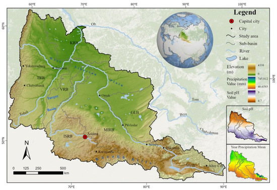
Figure 1.
An overview of the study area. MIRB: Middle Irtysh River Basin; TRB: Tobol River Basin; ISRB: Ishim River Basin; VRB: Vagai River Basin; GLB: Gorkoye Lake Basin.
2.2. Datasets
The data and its information used in this study can be found in Table 1.

Table 1.
Summary of the datasets.
Remote sensing data: The MODIS images come from the GEE platform, including MOD09A1, MOD11A2, and MOD13Q1.
Natural factor data: The DEM data is a Multi-Error-Removed Improved-Terrain DEM, which is used by ArcGIS to generate slope and aspect [68]. The total precipitation per year data comes from the ERA5 MONTHLY data of the European Centre for Medium-Range Weather Forecasts [69]. The soil data comes from the soil information provided by the International Soil Reference and Information Center (ISRIC), including bulk density (bdod), cation exchange capacity at pH 7 (cec), coarse fragments (cfvo), clay (clay), total nitrogen (nitrogen), pH in H2O (phh2o), sand (sand), and silt (silt) [70].
Human factor data: The population density data comes from The Gridded Population of the World, Version 4 (GPWv4) of the United Nations World Population Prospects data [71]. The value in each cell represents the population density of that cell.
2.3. Methodology
This study proposes a research framework to explore the interaction between the natural environment and human activities on EQ (Figure 2). Human activities accelerate the degradation of EQ. At the same time, the natural environment, including climate, soil, and topography, is an important component of EQ. Using the IRB as an example, this study uses the ARSEI to assess and analyze EQ at a large spatial scale. The introduction of the LandTrendr and PLUS models allows for the analysis of EQ changes in both space and time at the pixel level, investigating the driving factors and their role in influencing EQ variations.
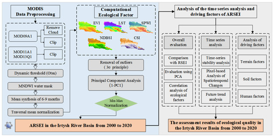
Figure 2.
Overall technical flow chart.
2.3.1. Construction of the ARSEI
In the watershed ecosystem, there is a close relationship between the different ecological factors, which promote and restrict each other and act together on the ecology of the watershed. How to determine the correlation between each ecological factor and the weight of its effect on the ecosystem becomes the key point when assessing EQ with multiple ecological factors. PCA can automatically and objectively determine its weight according to the contribution of each indicator to each principal component, thereby effectively reducing the range of data while retaining the maximum amount of information. To comprehensively monitor and evaluate the EQ of the watershed, this paper also selects PCA as the coupling method for five ecological factors, such as greenness, humidity, heat, dryness, and salinity, to construct the ARSEI (Table 2).
Table 2.
Summary of calculation methods for ecological factors.
(1) Greenness: The spatial distribution pattern of vegetation in the study area is a high vegetation cover area with dense forest in the north and a low vegetation cover area with grassland and cultivated land in the south. Thus, EVI is chosen as the greenness factor to avoid the weaknesses of NDVI, which is quickly saturated in heavily vegetated areas and easily influenced by the soil background in sparsely vegetated areas [72].
(2) Humidity: This paper uses the Surface Potential Water Abundance Index (SPWI) as the humidity factor. It uses the normalized index method to calculate the NIR and SWIR-2 bands while adding the blue band to adjust the index value, which can correctly reflect the abundance of surface water resources compared to wetness (WET) [73].
(3) Heat: Land surface temperature (LST) is not only a measure of climate change and land desertification in ecological terms but also one of the parameters characterizing surface aridity.
(4) Dryness: The Normalized Differential Build-up and Bare Soil Index (NDBSI) expresses the dryness factor. It is obtained by averaging the Soil Index (SI) and the Index-based Build-up Index (IBI) [26].
(5) Salinity: Instead of a single salinity index, the Comprehensive Salinity Index (CSI) is used in this paper. It more accurately reflects the ecological impact of salinity on a large scale (soil heterogeneity and land use type differences are obvious). The CSI is based on the idea of integrated learning and integrates three universal salinity indices: the Salinity Index (SI-T), the Normalized Differential Salinity Index (NDSI), and the Salinity Index 3 (SI3) to improve the stability and reliability of the detection results [32].
This study implemented the dynamic thresholding MNDWI method for water extraction by introducing the Otsu algorithm and generating a water mask. The use of precise water masks for each period improved the accuracy of the ARSEI results [34,35,36]. To avoid weight imbalances due to dimensional inconsistencies, it is imperative that each ecological factor be traversed and normalized to the range [0, 1] prior to PCA. Then, according to the “” principle of a normal distribution, the interval can effectively eliminate outliers among pixels. Then, the processed ecological factors are used as bands to synthesize multi-band images for PCA. The formula for PCA is as follows:
where represents the PCA operation; is the obtained principal component; is the first principal component; and the ARSEI is the ultimate result of PC1, with its values representing the assessment outcomes of EQ. High values indicate better EQ, while low values suggest poorer EQ.
To support the measurement and comparison of ecological quality, the min-max normalization method adjusts the ARSEI to [0,1]. When the ARSEI is close to 1, it reflects a higher level of ecological quality, and when it is further away, the quality is lower. The formula is as follows:
where indicates the normalized ARSEI, is the maximum value of the ARSEI, and is the minimum value of the ARSEI.
2.3.2. Time Series Stability Analysis
The coefficient of variation (CV) is the ratio of the standard deviation to the mean, which is a measure of the variability relative to the mean. It is free of units of measurement and is often used to measure the dispersion of data and to compare them with each other [74,75,76]. In this paper, it is used to reflect the degree of dispersion of the ARSEI and to assess the inter-annual time series stability of the ARSEI. The larger the CV value, the more discrete the distribution of the ARSEI and the greater the inter-annual variation. Otherwise, the concentrated distribution of the ARSEI and the smaller inter-annual fluctuation are the results. The calculation is shown below:
where is the standard deviation of the ARSEI and is the mean of the ARSEI.
2.3.3. Spatiotemporal Change Detection Algorithm of the ARSEI
LandTrendr, utilizing an annual time series decomposition algorithm, identifies vegetation trends through spectral pixel trajectories (Figure 3). In this study, LandTrendr was used to investigate the degradation (loss) and improvement (gain) of EQ on an inter-annual scale. LandTrendr is now operational in Google Earth Engine (LT-GEE), significantly improving processing efficiency [51]. The parameters of LT-GEE can be found in the supplementary material (Table S1).

Figure 3.
Example of LandTrendr segmentation and fitting of the ARSEI time series. (a) A line chart with the selected point (Longitude: 61°22′23.90′′E, Latitude: 60°37′58.63′′N), original ARSEI values, and corresponding fitted values; (b) MODIS LUCC in 2001, 2005, 2010, 2015, and 2020; (c) an example of ARSEI changes in the years corresponding to MODIS LUCC.
2.3.4. Future Trend Analysis
This paper uses Theil-Sen median trend analysis coupled with a Mann-Kendall test to analyze future ARSEI trends in the IRB. It has been successfully applied in various studies related to hydrological and meteorological trend changes [77,78]. Theil-Sen median has the advantages of not being affected by missing data, being insensitive to measurement errors and outlier data, and having high computational efficiency [79,80]. It was calculated as follows:
where is the Theil-Sen median slope; Median is the median function; the ARSEI inclines when , and the ARSEI declines when .
Mann-Kendall is a non-parametric test. This parametric test method is more appropriate for ordinal variables as it does not require samples to be drawn from a specified distribution and is less susceptible to outliers. The statistical significance of the Theil-Sen trend analysis is defined by the Z-value of MK. If the magnitude of Z is greater than 1.65 and 1.96, it means that the trend has passed the significance test with 90% and 95% confidence, respectively (Table 3). It is calculated as follows:
In the formula, is a sign function, n is the amount of data in the sequence, and S is the test statistic when is the significant change in the ARSEI studied at a given significant level α.
Table 3.
Classification table of the Sen-MK trend and Hurst index changes.
The Hurst index is a numerical measure of the persistence of time series data used in hydrology, economics, and climatology [81,82]. In this paper, the Hurst index was calculated using the rescaled polar difference R/S analysis to analyze the persistence of future change trends of the ARSEI in the IRB, which can better express the inter-annual variability characteristics. For example, 0 < H < 0.5 represents the inverse persistence of the time series data, i.e., the future change trend is opposite to the past trend; H = 0.5 represents the randomness of the time series data, i.e., the future change trend is not correlated with the past; and 0.5 < H < 1 shows the time series data has persistence, i.e., the future trend is consistent with the past trend. The Theil-Sen median trend analysis and the Mann-Kendall test (Sen-MK) and Hurst indices were combined to analyze the persistence of the ARSEI change trends (Table 3).
2.3.5. Analysis of Driving Factors
The analysis of the drivers of EQ change is based on the PLUS model [59]. It integrates a rule mining framework based on the LEAS and a CA model based on multi-type random seeds (CARS). By analyzing different types of land use expansion and driving factors, the evolution of the probability of different types of land use and the contribution of driving factors to different types of land use expansion during this period can be obtained, and land use patches and land use scenario simulations can be predicted. In this paper, the LEAS explores the contribution of different driving factors to the hierarchical expansion of EQ and evaluates the role of each driving factor in the change in EQ in the IRB. The formula is as follows:
where is the development probability of land type k in unit i; x is a vector composed of multiple driving factors; I is the indicator function of the decision tree; is the prediction type of the nth decision tree of the vector x; and M is the total number of decision trees. When d is 1, it means that it converted other land use types to type k, and when d is 0, it means other transitions.
3. Results
3.1. Performance Evaluation of the ARSEI in the IRB
3.1.1. Advantages and Applicability of the ARSEI
To visually demonstrate the suitability of the proposed ARSEI compared to the conventional RSEI, we first select several typical areas in the IRB for the experimental analysis in Figure 4. From the results, it can be easily seen that: (1) compared to the RSEI, the ARSEI can more accurately reflect the real surface conditions near the water; and (2) compared to the RSEI, the ARSEI can better reflect the real EQ.
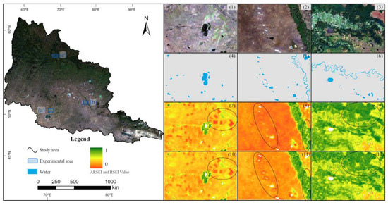
Figure 4.
Comparison of real remote sensing images, ESRI topographic maps, the ARSEI, and the RSEI for experimental areas (a), (b), and (c). (1–3) correspond to Landsat8 RS images of regions (a), (b), and (c); (4–6) correspond to the ASTER Global Water Bodies Database for regions (a), (b), and (c); (7–9) correspond to the ARSEI of the regions (a), (b), and (c); and (10–12) correspond to the RSEI of the regions (a), (b), and (c).
The greenness index in the RSEI is represented using the NDVI, which tends to saturate in areas with high vegetation cover and is susceptible to soil influence in regions with low vegetation cover. The ARSEI addresses these issues by employing the EVI and introducing the CSI as a salinity index to better reflect conditions in the arid regions of the IRB in Central Asia. By comparing the ARSEI and the RSEI using Landsat 8 RS imagery and the ASTER Global Water Database as benchmarks, the following conclusions are deduced [83,84]. A comparison of Figure 4(7,10) reveals that the ARSEI, while accurately representing vegetation greenness, also more precisely reflects the ecological quality of agricultural lands under the influence of soil salinity. Further comparison using Figure 4(8,11) indicates that the RSEI tends to overestimate the ecological degradation around salt lakes and does not adequately capture the impact of soil salinity on EQ. In contrast, Figure 4(8) illustrates how the ARSEI, through the CSI indicator, effectively represents the effect of soil salinity on EQ, showcasing the superiority of the CSI index within the ARSEI. Additionally, in high-value vegetation areas, as depicted in (b) and (c), the ARSEI finely details the ecological textures near river channels, identifying low-quality ecological points within the channels. Comparisons of Figure 4(9,12) demonstrate the ARSEI’s capability to comprehensively reflect the overall state of forests in the upper right section of the (c) test area, contrary to the RSEI, which displays fragmented patterns. A comparison with Landsat 8 imagery confirms that the ARSEI’s outcomes align more closely with the actual ground conditions. This analysis substantiates the accuracy and superiority of the ARSEI in assessing EQ.
3.1.2. Correlation Evaluation of Ecological Factors
The PCA results and the water threshold for each year from 2000 to 2020 can be found in the supplementary material (Table S2). The PCA results of five selected periods showed that the contribution rate of PC1 from 2000 to 2020 exceeded 88%, integrating most of the information on each ecological factor (Table 4). The loadings of each ecological factor in PC1 are stable and regular across years, with positive values for the EVI and the SPWI indicating that greenness and soil moisture had a positive effect on the ecology of the IRB and negative values for the LST, NDBSI, and CSI indicating that temperature, drought, and soil salinity had a negative effect on the ecology of the IRB. In contrast, the loadings of the other principal components were unstable and could not be used to characterize ecological importance.
Table 4.
The PCA results and the water threshold of five indicators.
To comprehensively assess the influence of the selected ecological factors on this catchment and validate their correlation with the PCA results, we performed a Pearson correlation analysis between the five ecological factors and the ARSEI (Figure 5). The correlation analysis results are illustrated in Figure 4. Notably, the EVI, SPWI, and ARSEI exhibited a positive correlation, while the LST, NDBSI, CSI, and ARSEI demonstrated a negative correlation, aligning with the PCA findings. The average correlation across the five periods for each ecological factor exceeded 0.69, and the correlation between each indicator and the ARSEI surpassed 0.79. These results affirm that the ARSEI effectively encapsulates the comprehensive information of each ecological factor, providing a holistic reflection of the overall EQ.
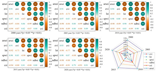
Figure 5.
Statistical chart of the correlation between the five indicators and the ARSEI. *: indicates a significance level of 0.05; **: indicates a significance level of 0.01. The average correlation is calculated by the absolute value of the correlation coefficient between a certain indicator and other indicators. Take EVI 2020 as an example: .
3.2. Ecological Environment Measurement Based on the ARSEI
The statistical results show that the ARSEI values in 2000–2020 are distributed in the range [0, 1], with an overall mean of around 0.54, a median in the range 0.48–0.58, and a standard deviation of 0.23, which is subject to some fluctuation (Figure 6). In terms of the density frequency distribution, the high density of the ARSEI values is concentrated in the range of 0.11–0.90, showing a bimodal distribution. This feature statistically highlights an imbalance in the EQ of the IRB.
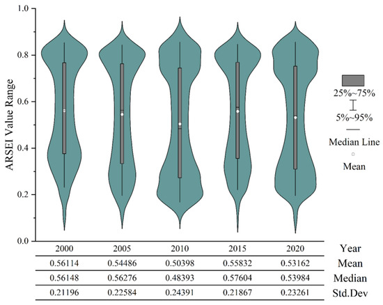
Figure 6.
Statistics of the ARSEI in the IRB from 2000 to 2020.
To quantitatively depict the spatial EQ of the study area, the ARSEI results were categorized into five levels (I-V) for precise quantification and visualization: poor (0.0–0.2), fair (0.2–0.4), average (0.4–0.6), good (0.6–0.8), and excellent (0.8–1.0) (Figure 7).
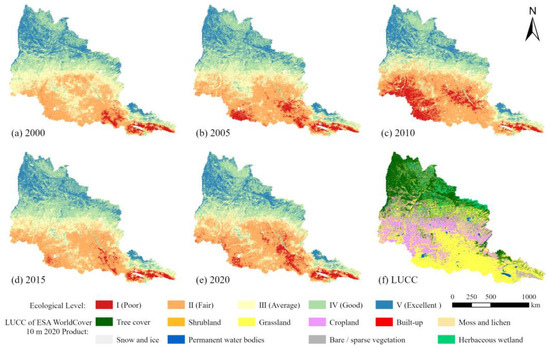
Figure 7.
Classification maps of ecological quality and LUCC in the IRB.
In general, there is evident spatial heterogeneity in the ecological environment of the IRB. Using approximately 55°N as a boundary, EQ is generally better in the north, while EQ is generally worse in the south. The distribution pattern gradually improves from south-east to north-west. The areas with an overall better EQ are Russia and the northern slopes of the Altay Mountains in Xinjiang, China, where forests, herbaceous wetlands, and shrubs predominate. Areas of medium EQ are mainly located on the border between Russia and Kazakhstan, where grassland and cultivated land predominate. The EQ is poor in Kazakhstan and on the southern slopes of the Altay Mountains in the IRB. Combined with the land use classification, forests and shrubs are distributed in level V; shrubs, grasslands, and herbaceous wetlands in level Ⅳ; mainly grassland and cultivated land in levels Ⅲ and Ⅱ; and grassland, bare land, and alpine ice and snow in level Ⅰ (Figure 7f).
The study used a gravity transfer model to calculate the coordinates of the center of gravity for levels I–V between 2000 and 2020 and to plot the transfer path (Figure 8). The results show that the movement trends for levels I and II are from south-east to north-west. Conversely, the movement trends for levels III and IV are from south-west to north-east, while the transfer path of level V involves an initial movement to the south-east, followed by a shift to the north-west, and finally a downward movement from 2015 to 2020. The distances traveled for levels I to V are 1798 km, 199 km, 268 km, 165 km, and 98 km, respectively.
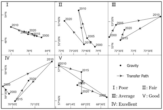
Figure 8.
Gravity transfer path map.
The transfer matrix further reflects the difference in the spatiotemporal distribution of the EQ pattern (Figure 9). Over the last 20 years, EQ in the IRB has shown an overall trend of deterioration followed by improvement. From 2000 to 2005, there were few transfers between different classes, but after 2005, transfers between classes became more frequent. The level IV and V areas showed relatively stable changes; the level III area showed a deteriorating trend; the level II area showed an increasing trend; and the level I area initially increased but then decreased.
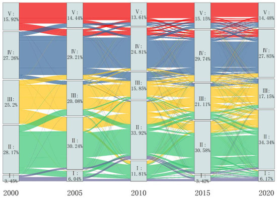
Figure 9.
ARSEI transfer matrix and the proportion of each ecological level for the IRB from 2000–2020.
3.3. Time Series Analysis of Ecological Quality in the Irtysh River Basin
3.3.1. Time Series Stability Analysis
To study the spatial variation characteristics of EQ from 2000 to 2020 in more detail, a pixel-scale spatial measurement and a temporal evolution stability simulation were carried out to obtain the ARSEI coefficient of variation (CV) (Figure 10). Its values are mainly concentrated at 0~0.2, accounting for 87.5%, indicating that the overall fluctuation of the ARSEI is small and in a stable state.
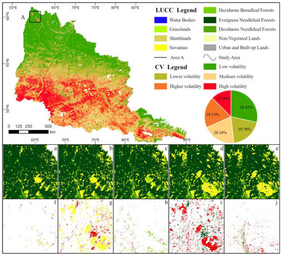
Figure 10.
ARSEI stability grading map of the Irtysh River Basin from 2000 to 2020. Images a-e correspond to MODIS_LC_Type3 in 2001, 2005, 2010, 2015, and 2020, respectively. Changes in major LUCC types from 2001 to 2020 (red represents a decrease and other colors represent an increase): f. bush, g. savannah, h. deciduous broadleaf forest, i. evergreen coniferous forest, and j. deciduous coniferous forest.
The area distribution across different variability classes is as follows, in descending order of proportion: low variability at 28.43%, medium variability at 20.16%, lower variability at 19.78%, higher variability at 19.13%, and high variability at 12.50%. The range of the coefficient of variation is 0.0104~1.0294, the mean is 0.1115, and the standard deviation is 0.0734. The spatial distribution of each fluctuation level shows that there is significant spatial heterogeneity in the EQ of the catchment. The low-variability areas are mainly distributed in the West-Siberian plains of Russia in the northern part of the catchment, and the high-variability areas are mainly distributed in the northern Kazakh hills and the Turgai depression in Kazakhstan. The forest ecosystem has a low degree of variability, while the grassland and cropland ecosystems have a high degree of variability. However, even forest areas with low EQ variability experience local fluctuations. For example, the area change in LUCC shows that the extent of evergreen needle-leaf forests decreases and the area of shrublands and savannas increases from 2001 to 2020, causing major changes in EQ in the area in the northern part of A.
3.3.2. Pixel-Based Analysis of Spatiotemporal Changes in Ecological Quality
This study uses LT-GEE to analyze the greatest loss and gain of spatiotemporal change in EQ on a pixel basis (Figure 11). The interannual loss analysis of EQ shows that the distribution areas of levels II (fair) and III (average) are the main areas where loss and gain occur. The EQ inter-annual loss analysis reveals that the south-western part of the basin, particularly the northern region of Kazakhstan, experiences more prolonged and substantial losses. In the time series stability analysis, region A in the northern part of the basin is identified as an area with severe and sustained losses over approximately 20 years (Figure 11c). The loss time plot shows that the decline in EQ is more pronounced in 2000–2005, and the end of the loss is more pronounced in 2005–2012 (Figure 11a–c). The analysis of the inter-annual growth of EQ shows that the area of gain growth coincides very closely with the area of loss. In the Kazakhstan-Russia border region, the period of gain is around 2000–2002, and within Kazakhstan, the period of gain is around 2012–2020, with most of the growth lasting only one year (Figure 11d–f).
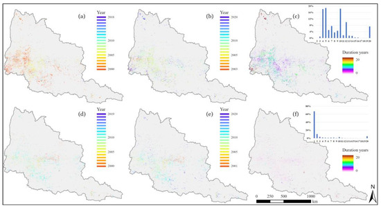
Figure 11.
Spatiotemporal loss/gain of ecological quality in the IRB from 2000 to 2020. Different colors represent different years. (a) start time of the loss; (b) end time of the loss; (c) duration of the loss; (d) start time of the gain; (e) end time of the gain; and (f) duration of the gain.
3.3.3. Future Trend and Persistence Analysis
The Sen-MK and the Hurst index were used to quantify the spatial distribution characteristics of trend changes and the persistence of EQ in the study area (Figure 12). The results of future trend analysis, at a confidence level of α = 0.05, reveal distinct patterns: areas exhibiting an advancing EQ trend (composed of significant and slight improvements) constitute 14.71%, those with a consistent EQ trend (remaining stable without change) make up 76.15%, and regions witnessing a declining EQ trend (marked by significant and slight deteriorations) account for 9.14%. The Hurst index ranges from 0.053 to 1, with an average of 0.433. The portion with values below 0.5 represents 76.58% of the total area, while values above 0.5 represent only 23.42%. This suggests a robust negative persistence in the trend of EQ change within the IRB, implying that the trajectory of EQ change in most catchments will be opposite to that of the past. The regions with a Hurst index of less than 0.5 are mainly located in areas of levels Ⅰ-Ⅲ, indicating that the EQ of the catchment is gradually improving. It is worth noting that in the southern part of the Pavlodar region, the EQ classification typically falls within levels I or II, with a Hurst value less than 0.5. This suggests that the region is likely to encounter challenges in transitioning toward an improving trend.
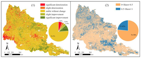
Figure 12.
Trend analysis and persistence distribution of the ARSEI in the IRB from 2000 to 2020. (1) Trend analysis by the Sen-MK; (2) future trend persistence analysis by the Hurst index.
The results of the Sen-MK analysis were combined with the Hurst index to analyze the persistence of future changes in the trend in EQ in the study area (Table 3). The analysis revealed the following distribution of results: 76.15% for persistent and stable conditions, 7.47% for persistent and significant improvement, and 4.36% for persistent and significant degradation. This was followed by 3.14% showing a trend from persistent and significant improvement to persistent and significant degradation, 3.08% for persistent and slight improvement, 2.55% for persistent and slight degradation, 1.53% for a shift from persistent and significant degradation to persistent and significant improvement, 1.02% for transitioning from persistent and slight improvement to persistent and slight degradation, and finally, 0.71% for persistent slight degradation evolving into persistent slight improvement (Figure 13). This indicates that the future trend of the ARSEI in the basin is dominated by persistent stability in the average, with an overall improvement in EQ. The spatial distribution of sustainable changes in future trends in EQ shows that the West Siberian Plain and the northern slopes of the Altay Mountains and East Kazakhstan Oblast continue to show significant improvements in EQ, while the northern part of Pavlodar Oblast and Kostanay Oblast continue to show significant degradation.
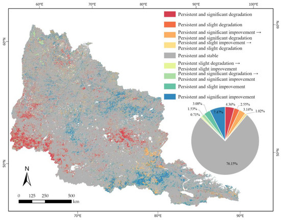
Figure 13.
Sustainability distribution of the ARSEI trend changes in the Irtysh River Basin from 2000 to 2020.
3.4. Analysis of Driving Factors for Ecological Quality in the Irtysh River Basin
This paper uses the PLUS model to analyze the driving forces of EQ changes at levels I–V). The PLUS model uses uniform sampling with 50 regression trees in Random Forest Regression (RFR) and a sampling rate of 0.1. The root mean square error (RMSE) values for levels I–V are 0.057, 0.091, 0.091, 0.097, and 0.079, respectively. In addition, out-of-bag (OOB) RMSE values of 0.165, 0.263, 0.264, 0.280, and 0.227, respectively, are also reported for the same categories. These data clearly demonstrate the effectiveness of the PLUS model, with minimal error in assessing the factors contributing to different types of environmental quality.
The poor area expansion is mainly driven by precipitation, elevation, and population density (Figure 14). Expansion occurs mainly in the southernmost part of the West-Siberian Plain, situated south of the Turgai Depression (Figure 15a). The main drivers of the increase in the fair are precipitation, population density, and soil pH (Figure 14). It increases mainly in the northern part of the territory of Kazakhstan, where the average annual precipitation from June to September is low (Figure 15b). The main drivers of average area expansion are population density, precipitation, and elevation (Figure 14). It increases mainly in the less densely populated areas, with an overall trend from northeast to southwest (Figure 15c). The main drivers of good area expansion are soil pH, precipitation, and elevation (Figure 14). The expansion area is in the north-central part of the basin and is characterized by slightly acidic soils with a pH range of 5.7–6.4. It shows a spatial pattern of increasing and then decreasing from south to north (Figure 15d). The predominant factors contributing to its excellent distribution are soil pH, precipitation, and elevation (Figure 14). It occurs mainly in the northern part of the watershed (Figure 15e).

Figure 14.
The contribution degree of driving factors of the ARSEI grade expansion in the Irtysh River Basin.

Figure 15.
The most important factors overlapped with the expansion of each grade of the ARSEI in the IRB.
4. Discussion
4.1. Rationality and Superiority of the ARSEI
In this paper, the GEE platform is used to calculate the ARSEI, which avoids the influence of pre-processing such as stitching and declouding on the results in software such as ENVI. The RSEI model has strong robustness and has been widely used in areas with different geographical conditions, with more than 1200 citations of related papers [85]. The ARSEI model improves the RSEI in three ways: (1) using the EVI to replace the NDVI; (2) adding a salinity factor that characterizes the soil environment for vegetation growth; and (3) using the Otsu algorithm to generate dynamic thresholds, which improve the accuracy of an EQ assessment using the IRB as an example. The ARSEI provides a more objective description of environmental realism than the RSEI results. The rationality of selected parameters has been clearly established with the Pearson correlation coefficient method. The analysis of the ARSEI results shows that it is not only consistent with the laws of ecological development (greenness, humidity, and productivity play a positive role in EQ; heat, dryness, and salinity play a negative role) but also with the results of various remote sensing ecological indices.
4.2. Spatiotemporal Pattern and Evolutionary Trend of Ecological Quality
The analysis of the spatial pattern and future trends of EQ in the IRB shows that the distribution of EQ exhibits pronounced spatial heterogeneity, with an overall spatial increase from south to north. The time series stability analysis shows that the EQ of the catchment is changing little and remains stable. The pixel-based analysis of spatiotemporal changes also indicates that within regions experiencing loss, there is a continuous process of gain. Simultaneously, the persistence of future trends suggests that EQ in the basin will show a slight trend towards improvement from a stable base.
The distribution areas of levels Ⅰ and Ⅱ are mainly located in arid areas of Central Asia, mainly grassland and cultivated land. Of these, EQ is very poor in the western part of Akmola Oblast, the north-western and western parts of Karaganda Oblast, and the areas around Zayan Lake in East Kazakhstan Oblast. The North Kazakhstan Oblast is the most stable and best-quality land use type in Kazakhstan, with an overall medium and above EQ. The East Kazakhstan Oblast and Pavlodar Oblast are typical industrial centers with numerous coal, non-ferrous metallurgy, oil, and chemical industry plants. These industries have a serious impact on soil, air, and rivers. The rapid development of these industries has led to serious environmental pollution [86]. A large amount of industrial wastewater is feared to be discharged into the Irtysh River every year, seriously affecting the EQ of the basin [87]. The Kostanay Oblast is the most typical area in the process of reclamation, abandonment, and then reclamation. According to the statistics, in the period 1988–2013, it had abandoned farmland, accounting for about 40% of the total area of its oblast [88]. Since 2000, exclusively land in the Kostanay Oblast with superior soil quality has been converted, resulting in further widespread land abandonment and degradation [88,89]. As human society encroaches on and alters the natural environment of this region, further ecological degradation is inevitable. The distribution area of level Ⅲ is mainly located on the border between Russia and Kazakhstan, where the main land use types are natural grassland and artificial cropland. The largest land type in North Kazakhstan Oblast is arable land, accounting for more than half of the total area. Grassland is another major land use type, accounting for about 30% of the total area. The conversion between these two types accelerates soil salinization, leading to ecological degradation. Abandoned arable land can accelerate the process of soil salinization through the growth of weeds and shrubs, leading to ecosystem degradation. In addition, the steps of southern West Siberia face a serious threat of water scarcity [90]. The distribution areas of levels Ⅳ and Ⅴ are mainly located in northern West Siberia. There are rich forests with high species richness that ensure the EQ of the area.
4.3. Analysis of Driving Factors for Ecological Quality
The driver factor analysis reveals that the ARSEI trend is consistent with the distribution of basin precipitation and soil pH and is negatively correlated with population distribution, while there is a clear gradient in the impact of altitude on EQ. Precipitation in the southern region indicates a decrease in EQ, while increased precipitation and slightly acidic soils favoring alpine forest vegetation in the northern region indicate an improvement in EQ. Human activities contribute to ecological degradation by converting land for agriculture and construction.
The reason for the decrease in EQ in the poor region is that the temperature increases and precipitation decreases, thereby exacerbating drought [91]. The region encompasses a mild gradient, large areas of cultivable land, and grassy terrain, rendering it a fitting ground for human settlement. A change in agricultural policy has markedly altered the landscape, transitioning cultivation grounds to grazing areas—a progression from cultivable to fallow, cut, pasture, and finally grazing lands, specifically within Akmola Oblast and Karaganda Oblast. Overutilization of grassland is a lasting challenge, as it is less productive than arable land. This results in alterations to the grassland ecosystem, causing a reduction in vegetation coverage, which subsequently becomes arid and saline. This leads to a significant decline in EQ [88,92].
The fair region has a typical continental climate, characterized not only by high radiation and large intra-annual temperature variations but also by considerable rainfall variability. It has many heavy rainfall events in the summer, sometimes reaching 24–65 mm or more in 24 hours. The heavy rainfall increases erosion and soil loss, while the high summer temperatures in the region lead to strong wind erosion due to the high evaporation of water after heavy rainfall [93]. According to Pavlodar Oblast statistics, 74% of arable land is affected by wind erosion. In Altayskiy Kray, 95% of the barren arable land is in the dry steppe zone bordering Kazakhstan [94]. This is because higher soil pH leads to lower species richness in the arid grasslands of northern Kazakhstan and south-western Siberia [95]. At the same time, the needs of people in Kazakhstan for economic and social development have led to overgrazing, land expansion, and mineral exploitation, resulting in increased soil erosion and pollution. Both adverse climatic and human influences are not conducive to improving EQ.
The impact of population density on EQ in average regions results from the development and use of urban and agricultural land. Kazakhstan’s urbanization efforts in the 21st century have exerted significant pressure on the ecological environment [96]. After independence, Kazakhstan began to restore natural pastures and rangeland that had been haphazardly cultivated. In the period 2000–2018, abandoned land and state-owned pastures were brought back to use. In 2006, Kazakhstan introduced the Sustainable Development Action Plan (2007–2024) and has continued to strengthen environmental protection efforts and improve relevant laws and regulations. It has achieved some useful results in ecological management and restoration, such as improving saline soils, seasonal grazing, and establishing nature reserves. As a result, the overall use of natural resources is better than in the past, and ecological conditions have improved.
The expansion of good regions is located in the north-central part of the basin, where increased precipitation has reduced soil pH to a slightly acidic range of 5.7–6.4, creating an environment for increased species richness [97]. The rate of forest restoration in Western Siberia is increasing because the President of the Russian Federation (No. 474 of 21 July 2020) established twelve national projects in 2018 [98]. In the Omsk region alone, about 8900 ha of forest will be restored and planted in 2020, increasing the forest cover and effectively restoring areas where forests have been degraded to shrubs or grassland because of overharvesting.
The excellent region is mainly distributed in the northern part of the IRB, which is the West Siberian Plain, with a large amount of coniferous and deciduous forests. The coniferous forests include spruce, pine, fir, and larch, while the deciduous forests include birch, poplar, willow, and kaiju. Research has shown that spruce and birch are suitable for soils with a pH of 5 to 7 and that this region provides a good ecological basis for forest regeneration [99]. The average precipitation from June to September every year is relatively high, and the abundant precipitation resources will further promote the improvement in EQ. It will further regulate deforestation in the region under Russia’s ecological protection policy. It will also find the best balance between EQ and economic benefits in the research area.
4.4. Limitations of the Study and Future Work
To complete an EQ assessment of the IRB, MODIS products were selected as the data source to reduce the computational requirements. However, it is important to recognize that the resolution of MODIS can affect the accuracy of EQ assessments. The selection of drivers is dominated by natural factors such as soil properties, rainfall, and topography. These indicators are key elements that influence EQ. The ARSEI shows that greenness and soil moisture are the most important contributors to EQ. There is a strong relationship between vegetation and soil. Soil and topography serve as the basis for vegetation growth, while precipitation affects its development. Therefore, we analyzed the driving mechanism of the above factors on the change in EQ. At the same time, these soil characteristics are easily obtained with GEE. Population density was chosen as a driving factor because the impact of human activities on the environment is becoming increasingly apparent. However, human activities are complex, and population density alone may not fully reflect the impact of human activities on the study area. Future work will focus on using higher-resolution datasets to improve the accuracy of the assessment and exploring the coupling relationship between human activities and the EQ of the IRB through additional human factors.
5. Conclusions
The ARSEI comprehensively, objectively, and quantitatively reflects the EQ of the IRB from 2000 to 2020 using remote sensing technology through the framework. Analysis of the temporal and spatial variations in its results leads to the following conclusions:
(1) The correlation between the ARSEI and each indicator reaches more than 0.88, which can effectively characterize EQ. Among them, EVI can express the vegetation cover of the catchment more accurately than NDVI. The EQ of the IRB displays significant spatial variation, with more impressive EQ in the northern areas and relatively inferior quality in the southern regions. The gradual improvement from south to north is exhibited by this spatial pattern.
(2) The ARSEI was used to assess the EQ of the IRB watershed, and the overall situation showed a stable state with small fluctuations. In the current research context, the continuity analysis of future trend changes in the EQ of the IRB watershed shows that it will continue to improve on a stable basis. Among these, arid grasslands are an area of significant and continuous improvement.
(3) Precipitation, soil pH, elevation, and human population are the main factors influencing the EQ of the IRB. Due to spatial heterogeneity, the driving factors for different EQ classes are different. Among them, precipitation has a more significant impact on EQ.
This study presents the ARSEI-based evaluation outcomes of EQ and its prospective alteration patterns, as well as investigating the drivers of diverse EQ categories. The findings of this investigation provide a theoretical framework that may be utilized for the formulation of ecological preservation, management, governance, and sustainable development strategies and practices.
Supplementary Materials
The following supporting information can be downloaded at: https://www.mdpi.com/article/10.3390/land13020222/s1, Table S1: The parameters of LT-GEE; Table S2: The PCA results and the water threshold for the IRB from 2000 to 2020; Table S3: Research paper formulas and parameters overview.
Author Contributions
Conceptualization, W.L. and A.S.; Funding acquisition, A.S. and J.A.; Investigation, W.L. and W.W.; Methodology, W.L.; Project administration, J.A. and A.S.; Software, W.L.; Supervision, A.S. and W.W.; Visualization, W.L. and A.S.; Writing—original draft, W.L.; Writing—review and editing, W.L. and A.S. All authors have read and agreed to the published version of the manuscript.
Funding
This research was funded by the Third Xinjiang Comprehensive Scientific Investigation Project under grant number 2022xjkk0702; the Western Young Scholars Project of the Chinese Academy of Sciences under grant number 2022-XBQNXZ-001; and the Tianshan Talent Development Program under grant number 2022TSYCCX0006.
Data Availability Statement
Data are available from the corresponding author upon reasonable request.
Acknowledgments
The authors are particularly grateful to all researchers and institutions for providing data support for this study. The authors would also like to thank the editors and reviewers for their valuable comments, which significantly helped improve the quality of this manuscript.
Conflicts of Interest
The authors declare no conflicts of interest.
References
- Framing and Context. Global Warming of 1.5 °C: IPCC Special Report on Impacts of Global Warming of 1.5 °C above Pre-industrial Levels in Context of Strengthening Response to Climate Change, Sustainable Development, and Efforts to Eradicate Poverty; Intergovernmental Panel on Climate Change (IPCC), Ed.; Cambridge University Press: Cambridge, UK, 2022; pp. 49–92. ISBN 978-1-00-915795-7. [Google Scholar]
- Arias, P.A.; Bellouin, N.; Coppola, E.; Jones, R.G.; Krinner, G.; Marotzke, J.; Naik, V.; Palmer, M.D.; Plattner, G.-K.; Ro-gelj, J.; et al. 2021: Technical Summary. In Climate Change 2021: The Physical Science Basis. Contribution of Working Group I to the Sixth Assessment Report of the Intergovernmental Panel on Climate Change. Masson-Delmotte, V., Zhai, P., Pirani, A., Connors, S.L., Péan, C., Ber-ger, S., Caud, N., Chen, Y., Goldfarb, L., Gomis, M.I., et al., Eds.; Cambridge University Press: Cambridge, UK; New York, NY, USA, 2023; pp. 33–144. [Google Scholar] [CrossRef]
- Cheng, G.; Li, X. Integrated Research Methods in Watershed Science. Sci. China Earth Sci. 2015, 58, 1159–1168. [Google Scholar] [CrossRef]
- Ye, S.; Pei, L.; He, L.; Xie, L.; Zhao, G.; Yuan, H.; Ding, X.; Pei, S.; Yang, S.; Li, X.; et al. Wetlands in China: Evolution, Carbon Sequestrations and Services, Threats, and Preservation/Restoration. Water 2022, 14, 1152. [Google Scholar] [CrossRef]
- Peters, R.L.; Lovejoy, T.E. Global Warming and Biological Diversity; Yale University Press: New Haven, CT, USA, 1992; ISBN 0-300-05930-2. [Google Scholar]
- Anderson, E.P.; Marengo, J.; Villalba, R.; Halloy, S.; Young, B.; Cordero, D.; Gast, F.; Jaimes, E.; Ruiz, D.; Herzog, S.K. Consequences of Climate Change for Ecosystems and Ecosystem Services in the Tropical Andes. Clim. Chang. Biodivers. Trop. Andes 2011, 1, 1–18. [Google Scholar]
- Li, S.Y.; Lei, J.Q. The Pattern and Change of the Ecosystems in the Ergis River Watershed. Arid. Zone Res. 2002, 19, 56–61. [Google Scholar]
- Huang, W.; Duan, W.; Nover, D.; Sahu, N.; Chen, Y. An Integrated Assessment of Surface Water Dynamics in the Irtysh River Basin during 1990–2019 and Exploratory Factor Analyses. J. Hydrol. 2021, 593, 125905. [Google Scholar] [CrossRef]
- Huang, W.; Duan, W.; Chen, Y. Rapidly Declining Surface and Terrestrial Water Resources in Central Asia Driven by Socio-Economic and Climatic Changes. Sci. Total Environ. 2021, 784, 147193. [Google Scholar] [CrossRef] [PubMed]
- Stoyashcheva, N.V.; Rybkina, I.D. Water Resources of the Ob-Irtysh River Basin and Their Use. Water Resour. 2014, 41, 1–7. [Google Scholar] [CrossRef]
- Huang, F.; Xia, Z.; Li, F.; Guo, L.; Yang, F. Hydrological Changes of the Irtysh River and the Possible Causes. Water Resour. Manag. 2012, 26, 3195–3208. [Google Scholar] [CrossRef]
- Wei, Z.; Shi-chang, K.; Yong-ping, S.; Jian-qiao, H.; An-an, C. Response of Snow Hydrological Processes to a Changing Climate during 1961 to 2016 in the Headwater of Irtysh River Basin, Chinese Altai Mountains. J. Mt. Sci. 2017, 14, 2295–2310. [Google Scholar] [CrossRef]
- Liu, Q.; Wu, S. Variation Characteristics of Diurnal Temperature and Influence Factors of Irtysh River in Xinjiang. J. Soil. Water Conserv. 2017, 31, 351–356. [Google Scholar]
- Yang, Y.; Wu, X.-J.; Liu, S.-W.; Xiao, C.-D.; Wang, X. Valuating Service Loss of Snow Cover in Irtysh River Basin. Adv. Clim. Chang. Res. 2019, 10, 109–114. [Google Scholar] [CrossRef]
- Chemagin, A.A. Dynamics of Distribution of Inconnu in the Riverbeds Depression of the Irtysh River. IOP Conf. Ser. Earth Environ. Sci. 2020, 539, 012185. [Google Scholar] [CrossRef]
- Liu, Y.-J.; Wang, X.-R.; Zeng, Q.-Y. De Novo Assembly of White Poplar Genome and Genetic Diversity of White Poplar Population in Irtysh River Basin in China. Sci. China Life Sci. 2019, 62, 609–618. [Google Scholar] [CrossRef] [PubMed]
- Tusupbekov, Z.A.; Ryapolova, N.L.; Nadtochiy, V.S. Assessment of Phytocenoses Ecological Potential in South of Western Siberia Based on Hydrological and Climatic Calculations to Increase Agricultural Production. IOP Conf. Ser. Earth Environ. Sci. 2021, 624, 12235. [Google Scholar] [CrossRef]
- Xi, B.W.; Barčák, D.; Oros, M.; Chen, K.; Xie, J. The Occurrence of the Common European Fish Cestode Caryophyllaeus Laticeps (Pallas, 1781) in the River Irtysh, China: A Morphological Characterization and Molecular Data. Acta Parasitol. 2016, 61, 493–499. [Google Scholar] [CrossRef] [PubMed]
- Fan, J.; Abudumanan, A.; Wang, L.; Zhou, D.; Wang, Z.; Liu, H. Dynamic Assessment and Sustainability Strategies of Ecological Security in the Irtysh River Basin of Xinjiang, China. Chin. Geogr. Sci. 2023, 33, 393–409. [Google Scholar] [CrossRef] [PubMed]
- Yang, H.; Yang, F.; Lu, H.; Su, S. Assessment of Wetland Ecosystem Health in Irtysh River. J. Arid. Land. Resour. Environ. 2014, 28, 149–154. [Google Scholar]
- Messer, L.C.; Jagai, J.S.; Rappazzo, K.M.; Lobdell, D.T. Construction of an Environmental Quality Index for Public Health Research. Environ. Health 2014, 13, 39. [Google Scholar] [CrossRef]
- Allegro, G.; Sciaky, R. Assessing the Potential Role of Ground Beetles (Coleoptera, Carabidae) as Bioindicators in Poplar Stands, with a Newly Proposed Ecological Index (FAI). For. Ecol. Manag. 2003, 175, 275–284. [Google Scholar] [CrossRef]
- Yu, H.; Zhao, J. The Impact of Environmental Conditions on Urban Eco-Sustainable Total Factor Productivity: A Case Study of 21 Cities in Guangdong Province, China. Int. J. Environ. Res. Public Health 2020, 17, 1329. [Google Scholar] [CrossRef]
- Gandhi, G.M.; Parthiban, S.; Thummalu, N.; Christy, A. Ndvi: Vegetation Change Detection Using Remote Sensing and Gis—A Case Study of Vellore District. Procedia Comput. Sci. 2015, 57, 1199–1210. [Google Scholar] [CrossRef]
- Gao, B.C. NDWI—A Normalized Difference Water Index for Remote Sensing of Vegetation Liquid Water from Space. Remote Sens. Environ. 1996, 58, 257–266. [Google Scholar] [CrossRef]
- Xu, H. A Remote Sensing Urban Ecological Index and Its Application. Acta Ecol. Sin. 2013, 33, 7853–7862. [Google Scholar]
- Hu, X.; Xu, H. A New Remote Sensing Index Based on the Pressure-State-Response Framework to Assess Regional Ecological Change. Environ. Sci. Pollut. R 2019, 26, 5381–5393. [Google Scholar] [CrossRef] [PubMed]
- Hu, X.; Xu, H. A New Remote Sensing Index for Assessing the Spatial Heterogeneity in Urban Ecological Quality: A Case from Fuzhou City, China. Ecol. Indic. 2018, 89, 11–21. [Google Scholar] [CrossRef]
- Wang, L.; Jiao, L.; Lai, F.; Zhang, N. Evaluation of Ecological Changes Based on a Remote Sensing Ecological Index in a Manas Lake Wetland, Xinjiang. Acta Ecol. Sin. 2019, 39, 2963–2972. [Google Scholar]
- Liu, Y.; Dang, C.; Yue, H.; Lyu, C.; Qian, J.; Zhu, R. Comparison between Modified Remote Sensing Ecological Index and RSEI. Natl. Remote Sens. Bull. 2022, 26, 683–697. [Google Scholar] [CrossRef]
- Song, M.J.; Luo, Y.Y.; Duan, L.M. Evaluation of Ecological Environment in the Xilin Gol Steppe Based on Modified Remote Sensing Ecological Index Model. Arid. Zone Res. 2019, 36, 1521. [Google Scholar]
- Zhang, W.; Du, P.; Guo, S.; Lin, C.; Zheng, H.; Fu, P. Enhanced Remote Sensing Ecological Index and Ecological Environment Evaluation in Arid Area. Natl. Remote Sens. Bull. 2022, 27, 299–317. [Google Scholar] [CrossRef]
- Zhu, D.; Chen, T.; Zhen, N.; Niu, R. Monitoring the Effects of Open-Pit Mining on the Eco-Environment Using a Moving Window-Based Remote Sensing Ecological Index. Environ. Sci. Pollut. R. 2020, 27, 15716–15728. [Google Scholar] [CrossRef]
- Xu, H.; Deng, W. Rationality Analysis of MRSEl and Its Difference with RSEl. Remote Sens. Technol. Appl. 2022, 37, 1–7. [Google Scholar]
- Xu, H. A Study on Information Extraction of Water Body with the Modified Normalized Difference Water Index (MNDWI). J. Remote Sens. 2021, 5, 589–595. [Google Scholar] [CrossRef]
- Bangira, T.; Alfieri, S.M.; Menenti, M.; van Niekerk, A. Comparing Thresholding with Machine Learning Classifiers for Mapping Complex Water. Remote Sens. 2019, 11, 1351. [Google Scholar] [CrossRef]
- Tran, K.H.; Menenti, M.; Jia, L. Surface Water Mapping and Flood Monitoring in the Mekong Delta Using Sentinel-1 SAR Time Series and Otsu Threshold. Remote Sens. 2022, 14, 5721. [Google Scholar] [CrossRef]
- Li, A.; Fan, M.; Qin, G.; Xu, Y.; Wang, H. Comparative Analysis of Machine Learning Algorithms in Automatic Identification and Extraction of Water Boundaries. Appl. Sci. 2021, 11, 10062. [Google Scholar] [CrossRef]
- Tamiminia, H.; Salehi, B.; Mahdianpari, M.; Quackenbush, L.; Adeli, S.; Brisco, B. Google Earth Engine for Geo-Big Data Applications: A Meta-Analysis and Systematic Review. ISPRS J. Photogramm. Remote Sens. 2020, 164, 152–170. [Google Scholar] [CrossRef]
- Cao, B.; Yang, X.; Qiu, J. Research Progress and Application of Remote Sensing Big Data Analysis Based on Google Earth Engine. Geospat. Inf. 2021, 19, 13–19+6. [Google Scholar]
- Wang, X.; Tian, J.; Li, X.; Wang, L.; Gong, H.; Chen, B.; Li, X.; Guo, J. Benefits of Google Earth Engine in Remote Sensing. J. Remote Sens. 2022, 26, 299–309. [Google Scholar] [CrossRef]
- Yang, Z.; Tian, J.; Su, W.; Wu, J.; Liu, J.; Liu, W.; Guo, R. Analysis of Ecological Environmental Quality Change in the Yellow River Basin Using the Remote-Sensing-Based Ecological Index. Sustainability 2022, 14, 10726. [Google Scholar] [CrossRef]
- Xiong, Y.; Xu, W.; Lu, N.; Huang, S.; Wu, C.; Wang, L.; Dai, F.; Kou, W. Assessment of Spatial–Temporal Changes of Ecological Environment Quality Based on RSEI and GEE: A Case Study in Erhai Lake Basin, Yunnan Province, China. Ecol. Indic. 2021, 125, 107518. [Google Scholar] [CrossRef]
- Wang, X.; Yao, X.; Jiang, C.; Duan, W. Dynamic Monitoring and Analysis of Factors Influencing Ecological Environment Quality in Northern Anhui, China, Based on the Google Earth Engine. Sci. Rep. 2022, 12, 20307. [Google Scholar] [CrossRef] [PubMed]
- Gong, C.; Lyu, F.; Wang, Y. Spatiotemporal Change and Drivers of Ecosystem Quality in the Loess Plateau Based on RSEI: A Case Study of Shanxi, China. Ecol. Indic. 2023, 155, 111060. [Google Scholar] [CrossRef]
- Yi, S.; Zhou, Y.; Zhang, J.; Li, Q.; Liu, Y.; Guo, Y.; Chen, Y. Spatial-Temporal Evolution and Motivation of Ecological Vulnerability Based on RSEI and GEE in the Jianghan Plain from 2000 to 2020. Front. Environ. Sci. 2023, 11, 1191532. [Google Scholar] [CrossRef]
- Xu, H.; Wang, M.; Shi, T.; Guan, H.; Fang, C.; Lin, Z. Prediction of Ecological Effects of Potential Population and Impervious Surface Increases Using a Remote Sensing Based Ecological Index (RSEI). Ecol. Indic. 2018, 93, 730–740. [Google Scholar] [CrossRef]
- DeVries, B.; Verbesselt, J.; Kooistra, L.; Herold, M. Robust Monitoring of Small-Scale Forest Disturbances in a Tropical Montane Forest Using Landsat Time Series. Remote Sens. Environ. 2015, 161, 107–121. [Google Scholar] [CrossRef]
- Dewi, R.S.; Bijker, W.; Stein, A. Change Vector Analysis to Monitor the Changes in Fuzzy Shorelines. Remote Sens. 2017, 9, 147. [Google Scholar] [CrossRef]
- Zhu, Z.; Woodcock, C.E. Continuous Change Detection and Classification of Land Cover Using All Available Landsat Data. Remote Sens. Environ. 2014, 144, 152–171. [Google Scholar] [CrossRef]
- Kennedy, R.E.; Yang, Z.; Gorelick, N.; Braaten, J.; Cavalcante, L.; Cohen, W.B.; Healey, S. Implementation of the LandTrendr Algorithm on Google Earth Engine. Remote Sens. 2018, 10, 691. [Google Scholar] [CrossRef]
- Wu, S.; Gao, X.; Lei, J.; Zhou, N.; Guo, Z.; Shang, B. Ecological Environment Quality Evaluation of the Sahel Region in Africa Based on Remote Sensing Ecological Index. J. Arid. Land. 2022, 14, 14–33. [Google Scholar] [CrossRef]
- Guo, G.; Wu, Z.; Chen, Y. Evaluation of Spatially Heterogeneous Driving Forces of the Urban Heat Environment Based on a Regression Tree Model. Sustain. Cities Soc. 2020, 54, 101960. [Google Scholar] [CrossRef]
- Chen, M.; Luo, Y.; Shen, Y.; Han, Z.; Cui, Y. Driving Force Analysis of Irrigation Water Consumption Using Principal Component Regression Analysis. Agric. Water Manag. 2020, 234, 106089. [Google Scholar] [CrossRef]
- He, Y.X.; Yi, G.H.; Zhang, T.B. The EVI Trends and Driving Factors in Red River Basin Affected by the “Corridor-Corridorbarrier” Function during 2000—2014. ACTA Ecol. Sin. 2018, 38, 2056–2064. [Google Scholar]
- Wang, Z.; Liang, L.; Sun, Z.; Wang, X. Spatiotemporal Differentiation and the Factors Influencing Urbanization and Ecological Environment Synergistic Effects within the Beijing-Tianjin-Hebei Urban Agglomeration. J. Environ. Manag. 2019, 243, 227–239. [Google Scholar] [CrossRef] [PubMed]
- Geng, J.; Yu, K.; Xie, Z.; Zhao, G.; Ai, J.; Yang, L.; Yang, H.; Liu, J. Analysis of Spatiotemporal Variation and Drivers of Ecological Quality in Fuzhou Based on RSEI. Remote Sens. 2022, 14, 4900. [Google Scholar] [CrossRef]
- Zhang, Z.; Song, Y.; Wu, P. Robust Geographical Detector. Int. J. Appl. Earth Obs. Geoinf. 2022, 109, 102782. [Google Scholar] [CrossRef]
- Liang, X.; Guan, Q.; Clarke, K.C.; Liu, S.; Wang, B.; Yao, Y. Understanding the Drivers of Sustainable Land Expansion Using a Patch-Generating Land Use Simulation (PLUS) Model: A Case Study in Wuhan, China. Comput. Environ. Urban. 2021, 85, 101569. [Google Scholar] [CrossRef]
- Radelyuk, I.; Zhang, L.; Assanov, D.; Maratova, G.; Tussupova, K. A State-of-the-Art and Future Perspectives of Transboundary Rivers in the Cold Climate—A Systematic Review of Irtysh River. J. Hydrol-Reg. Stud. 2022, 42, 101173. [Google Scholar] [CrossRef]
- Zhang, X.; Zhang, W.; Zhang, D. Effects of Human Activities on Carbon Storage in the Irtysh River Basin. Arid. Zone Res. 2023, 40, 1333. [Google Scholar] [CrossRef]
- Huang, F.; Xia, Z.; Guo, L.; Yang, F. Effects of reservoirs on seasonal discharge of Irtysh River measured by Lepage test. Water Sci. Eng. 2014, 7, 363–372. [Google Scholar]
- Hrkal, Z.; Gadalia, A.; Rigaudiere, P. Will the River Irtysh Survive the Year 2030? Impact of Long-Term Unsuitable Land Use and Water Management of the Upper Stretch of the River Catchment (North Kazakhstan). Environ. Geol 2006, 50, 717–723. [Google Scholar] [CrossRef]
- Zhao, X.; Wang, C.; Li, S.; Hou, W.; Zhang, S.; Han, G.; Pan, D.; Wang, P.; Cheng, Y.; Liu, G. Genetic Variation and Selection of Introduced Provenances of Siberian Pine (Pinus Sibirica) in Frigid Regions of the Greater Xing’an Range, Northeast China. J. For. Res. 2014, 25, 549–556. [Google Scholar] [CrossRef]
- Timoshok, E.E.; Timoshok, E.N.; Gureyeva, I.I. Ecological and Cenotic Features of the Old-Growth Pinus Sibirica Forests in the North-Chuya Glaciation Center, Russian Altai. Ukr J Ecol 2020, 10, 291–298. [Google Scholar] [CrossRef] [PubMed]
- Mao, H.U.; Feng, C.; You-ping, C. Responses of Radial Growth of Pinus Sibirica to Climate and Hydrology in Altay, Xinjiang, China. Chinese Journal of Applied Ecology. 2021, 32, 3609. [Google Scholar] [CrossRef]
- Jinping, X. For Man and Nature: Building a Community of Life Together. Peace 2021, 2, 14–15+13. [Google Scholar] [CrossRef]
- Yamazaki, D.; Ikeshima, D.; Tawatari, R.; Yamaguchi, T.; O’Loughlin, F.; Neal, J.C.; Sampson, C.C.; Kanae, S.; Bates, P.D. A High-Accuracy Map of Global Terrain Elevations. Geophys. Res. Lett. 2017, 44, 5844–5853. [Google Scholar] [CrossRef]
- Copernicus Climate Change Service ERA5 Monthly Averaged Data on Single Levels from 1979 to Present 2019. Available online: https://cds.climate.copernicus.eu/cdsapp#!/dataset/reanalysis-era5-single-levels-monthly-means?tab=overview (accessed on 25 October 2023).
- Hengl, T.; Mendes de Jesus, J.; Heuvelink, G.B.; Ruiperez Gonzalez, M.; Kilibarda, M.; Blagotić, A.; Shangguan, W.; Wright, M.N.; Geng, X.; Bauer-Marschallinger, B. SoilGrids250m: Global Gridded Soil Information Based on Machine Learning. PLoS ONE 2017, 12, e0169748. [Google Scholar] [CrossRef] [PubMed]
- Center for International Earth Science Information Network—CIESIN—Columbia University Gridded Population of the World, Version 4 (GPWv4): Population Density Adjusted to Match 2015 Revision UN WPP Country Totals, Revision 11 2018. Available online: https://sedac.ciesin.columbia.edu/data/set/gpw-v4-population-density-adjusted-to-2015-unwpp-country-totals-rev11 (accessed on 25 October 2023).
- Wang, Z.; Liu, C.; Alfredo, H. From AVHRR-NDVI to MODIS-EVI: Advances in Vegetation Index Research. Acta Ecol. Sin. 2003, 23, 979–987. [Google Scholar]
- Jiao, Z.; Sun, G.; Zhang, A.; Jia, X.; Huang, H.; Yao, Y. Water Benefit-Based Ecological Index for Urban Ecological Environment Quality Assessments. IEEE J. Sel. Top. Appl. Earth Obs. Remote Sens. 2021, 14, 7557–7569. [Google Scholar] [CrossRef]
- Yosboonruang, N.; Niwitpong, S.-A.; Niwitpong, S. Bayesian Computation for the Common Coefficient of Variation of Delta-Lognormal Distributions with Application to Common Rainfall Dispersion in Thailand. Peerj 2022, 10, e12858. [Google Scholar] [CrossRef]
- Kelley, K. Sample Size Planning for the Coefficient of Variation from the Accuracy in Parameter Estimation Approach. Behav. Res. Methods 2007, 39, 755–766. [Google Scholar] [CrossRef]
- Hong, C.; Jin, X.; Ren, J.; Gu, Z.; Zhou, Y. Satellite Data Indicates Multidimensional Variation of Agricultural Production in Land Consolidation Area. Sci. Total Environ. 2019, 653, 735–747. [Google Scholar] [CrossRef] [PubMed]
- Han, F.; Yan, J.; Ling, H. Variance of Vegetation Coverage and Its Sensitivity to Climatic Factors in the Irtysh River Basin. Peerj 2021, 9, e11334. [Google Scholar] [CrossRef]
- Yao, J.; Chen, Y.; Chen, J.; Zhao, Y.; Tuoliewubieke, D.; Li, J.; Yang, L.; Mao, W. Intensification of Extreme Precipitation in Arid Central Asia. J. Hydrol. 2021, 598, 125760. [Google Scholar] [CrossRef]
- Qi, S.; Chen, S.; Long, X.; An, X.; Zhang, M. Quantitative Contribution of Climate Change and Anthropological Activities to Vegetation Carbon Storage in the Dongting Lake Basin in the Last Two Decades. Adv. Space Res. 2023, 71, 845–868. [Google Scholar] [CrossRef]
- Wang, N.; Yu, J.; Zhu, L.; Wang, Y.; He, Z. Spatial Downscaling of Remote Sensing Precipitation Data in the Beijing-Tianjin-Hebei Region. J. Comput. Commun. 2021, 9, 191–202. [Google Scholar] [CrossRef]
- Tong, S.; Zhang, J.; Bao, Y.; Lai, Q.; Lian, X.; Li, N.; Bao, Y. Analyzing Vegetation Dynamic Trend on the Mongolian Plateau Based on the Hurst Exponent and Influencing Factors from 1982–2013. J. Geogr. Sci. 2018, 28, 595–610. [Google Scholar] [CrossRef]
- Tong, S.; Lai, Q.; Zhang, J.; Bao, Y.; Lusi, A.; Ma, Q.; Li, X.; Zhang, F. Spatiotemporal Drought Variability on the Mongolian Plateau from 1980–2014 Based on the SPEI-PM, Intensity Analysis and Hurst Exponent. Sci. Total Environ. 2018, 615, 1557–1565. [Google Scholar] [CrossRef] [PubMed]
- 83. Landsat Surface Reflectance Data, Version 1: Originally Posted April 20, 2015; Version 1.1: June 16, 2015; Version 1.1 Updated: March 27, 2019; Fact Sheet; U.S. Geological Survey Reston: Reston, VA, USA, 2015; p. 1.
- NASA/METI/AIST/Japan Spacesystems, and U.A.S.T. ASTER Global Digital Elevation Model V003. distributed by NASA EOSDIS Land Processes DAAC 2019. Available online: https://data.nasa.gov/dataset/ASTER-Global-Water-Bodies-Database-V001/iric-yb28/data?no_mobile=true (accessed on 25 October 2023).
- Xu, H.; Li, C.; Lin, M. Should RSEI Use PCA or kPCA? Geomat. Inf. Sci. Wuhan Univ. 2022, 48, 506–513. [Google Scholar]
- Aldangorovna, K.B. About the Problems of Ecology of Pavlodar Region. Interact. Sci. 2018, 67–69. [Google Scholar] [CrossRef]
- Dahl, C.; Kuralbayeva, K. Energy and the Environment in Kazakhstan. Energy Policy 2001, 29, 429–440. [Google Scholar] [CrossRef]
- Yan, H.; Lai, C.; Akshalov, K.; Qin, Y.; Hu, Y.; Zhen, L. Social Institution Changes and Their Ecological Impacts in Kazakhstan over the Past Hundred Years. Environ. Dev. 2020, 34, 100531. [Google Scholar] [CrossRef]
- Kraemer, R.; Prishchepov, A.V.; Müller, D.; Kuemmerle, T.; Radeloff, V.C.; Dara, A.; Terekhov, A.; Frühauf, M. Long-Term Agricultural Land-Cover Change and Potential for Cropland Expansion in the Former Virgin Lands Area of Kazakhstan. Environ. Res. Lett. 2015, 10, 054012. [Google Scholar] [CrossRef]
- Plyusnin, V. Ecological Safety of Siberia. Contemp. Probl. Ecol. 2014, 7, 597–603. [Google Scholar] [CrossRef]
- Zheleznova, I.; Gushchina, D.; Meiramov, Z.; Olchev, A. Temporal and Spatial Variability of Dryness Conditions in Kazakhstan during 1979–2021 Based on Reanalysis Data. Climate 2022, 10, 144. [Google Scholar] [CrossRef]
- Fan, B.; Luo, G.; Hu, Z.; Li, C.-f.; Han, Q.-f.; Wang, Y.-g.; Li, X.; Yan, Y. Land Resource Development and Utilization in Central Asia. Arid. Land. Geogr. 2012, 35, 928–937. [Google Scholar]
- Issanova, G.; Abuduwaili, J.; Long, M. Overview of Central Asian Environments; China Meteorogical Press: Beijing, China, 2015; pp. 18–60. ISBN 978-7-5029-6148-0. [Google Scholar]
- Krasnoyarova, B.A.; Orlova, I.V.; Plutalova, T.G.; Sharabarina, S.N. Landscape-Ecological Assessment of Dry Lands of the Russian-Kazakhstan Border Zone for Sustainable Land Use. Arid. Ecosyst. 2019, 9, 150–156. [Google Scholar] [CrossRef]
- Palpurina, S.; Wagner, V.; von Wehrden, H.; Hájek, M.; Horsák, M.; Brinkert, A.; Hölzel, N.; Wesche, K.; Kamp, J.; Hájková, P.; et al. The Relationship between Plant Species Richness and Soil pH Vanishes with Increasing Aridity across Eurasian Dry Grasslands. Glob. Ecol. Biogeogr. 2017, 26, 425–434. [Google Scholar] [CrossRef]
- Huang, J.; Na, Y.; Guo, Y. Spatiotemporal Characteristics and Driving Mechanism of the Coupling Coordination Degree of Urbanization and Ecological Environment in Kazakhstan. J. Geogr. Sci. 2020, 30, 1802–1824. [Google Scholar] [CrossRef]
- Chytrý, M.; Danihelka, J.; Ermakov, N.; Hájek, M.; Hájková, P.; Kočí, M.; Kubešová, S.; Lustyk, P.; Otýpková, Z.; Popov, D.; et al. Plant Species Richness in Continental Southern Siberia: Effects of pH and Climate in the Context of the Species Pool Hypothesis. Glob. Ecol. Biogeogr. 2007, 16, 668–678. [Google Scholar] [CrossRef]
- Babkina, L.N.; Skotarenko, O.V.; Kozin, M.N. Main Implementation Criteria of the Ecology National Project in Russian Regions. IOP Conf. Ser. Earth Environ. Sci. 2021, 723, 042060. [Google Scholar] [CrossRef]
- Yang Huan; Yin Chunying; Tang Bo; Zheng Donghui; Zhao Chunzhang; Li Dandan; Liu Qing Difference in Soil pH Values between Picea Asperata and Abies Faxoniana Stands in Subalpine Regions and a Preliminary Study on Its Mechanism. Acta Ecol. Sin. 2018, 38, 5017–5026.
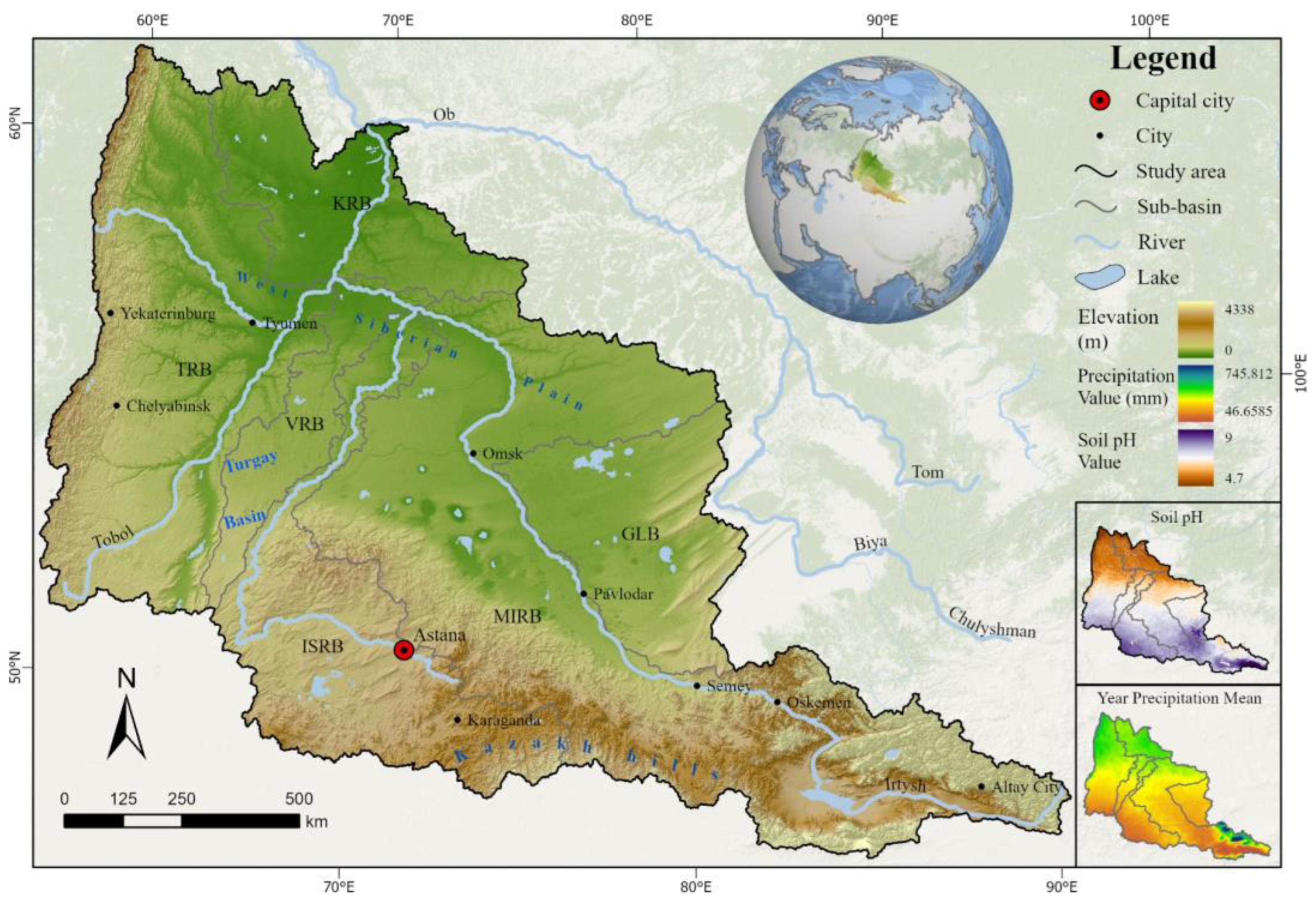
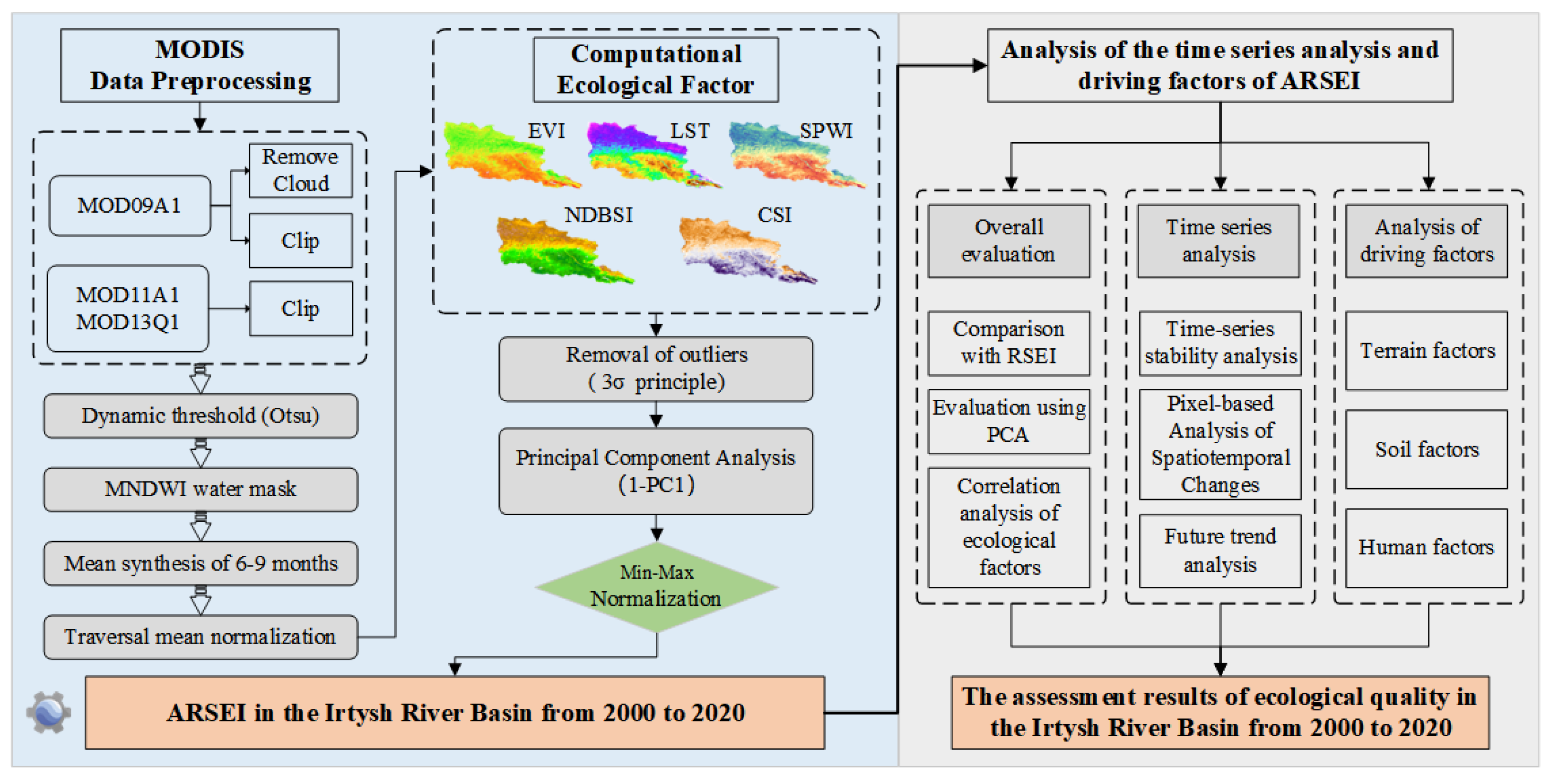
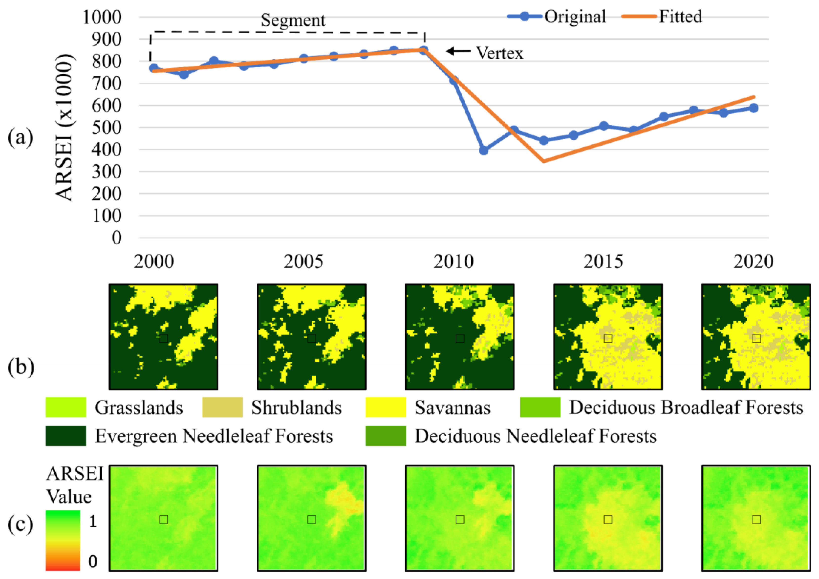
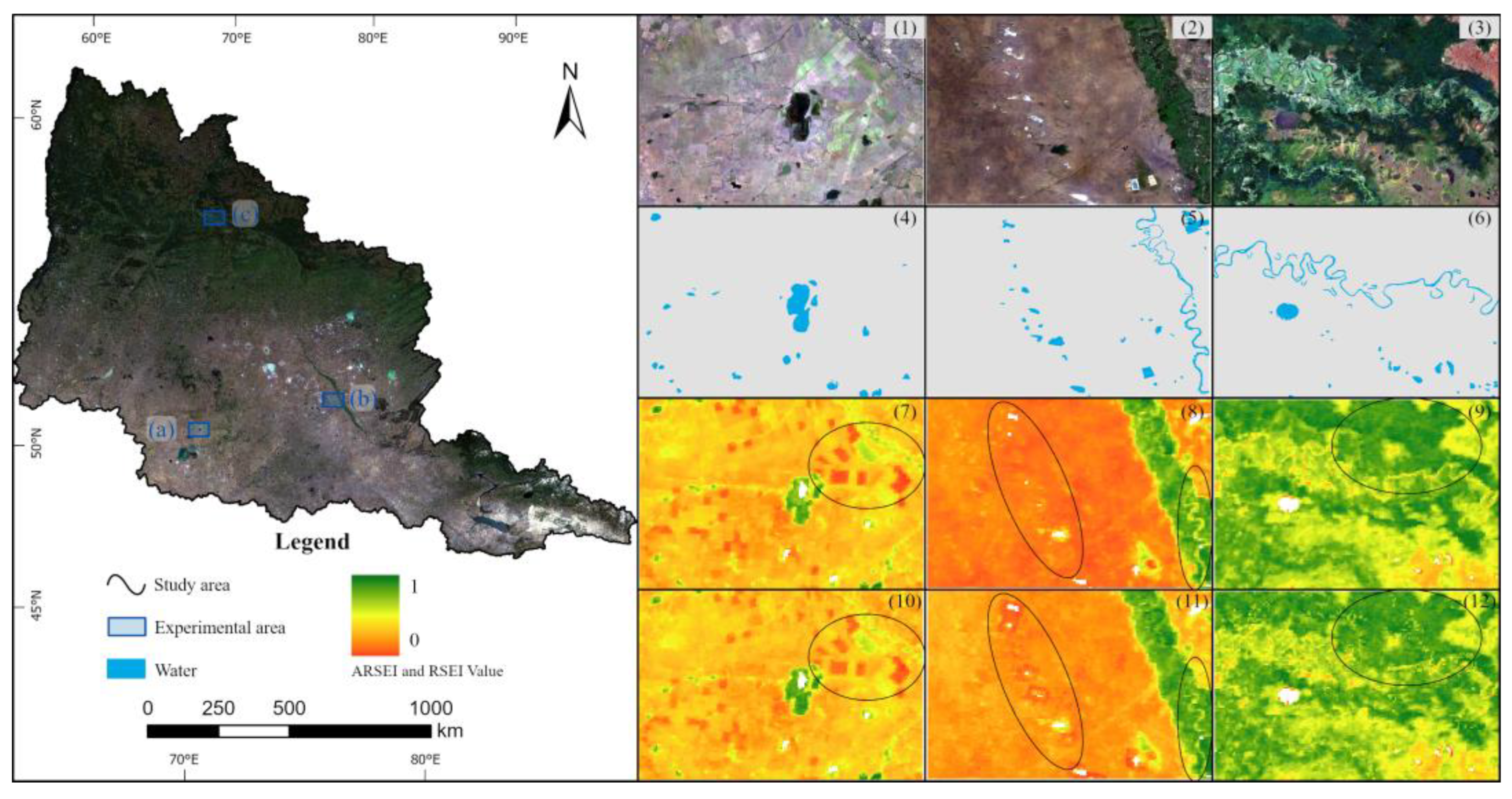

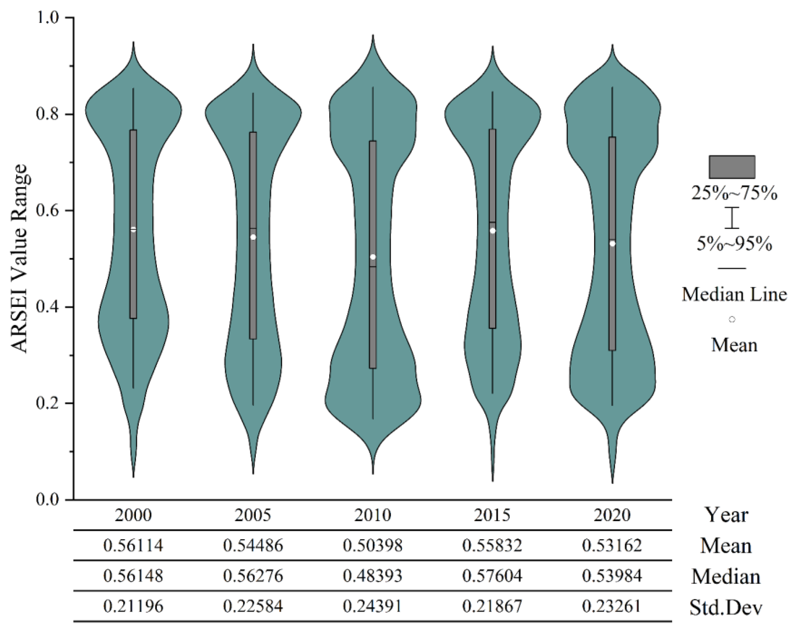


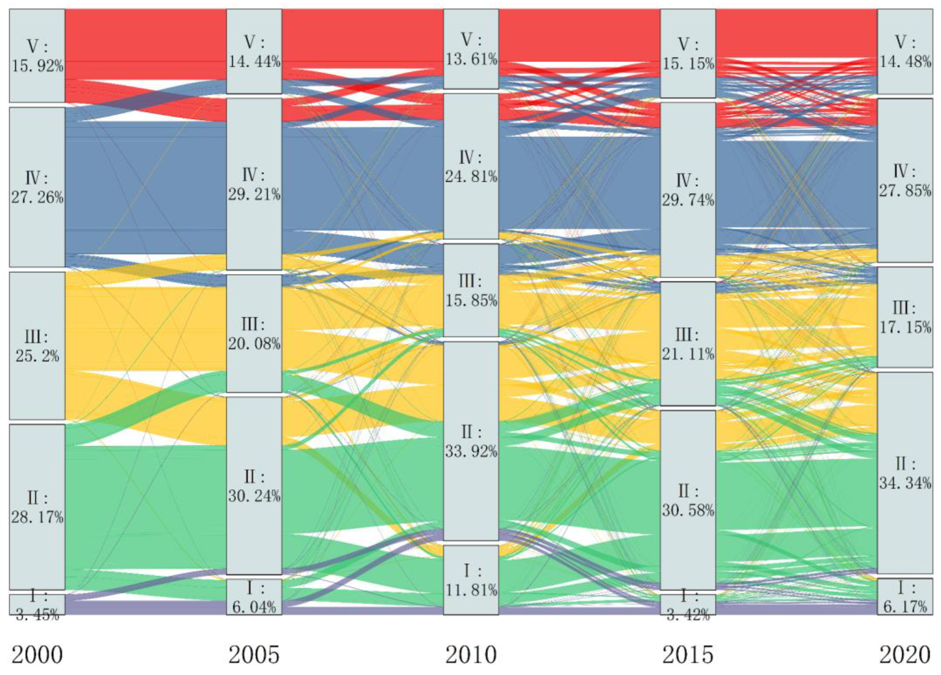
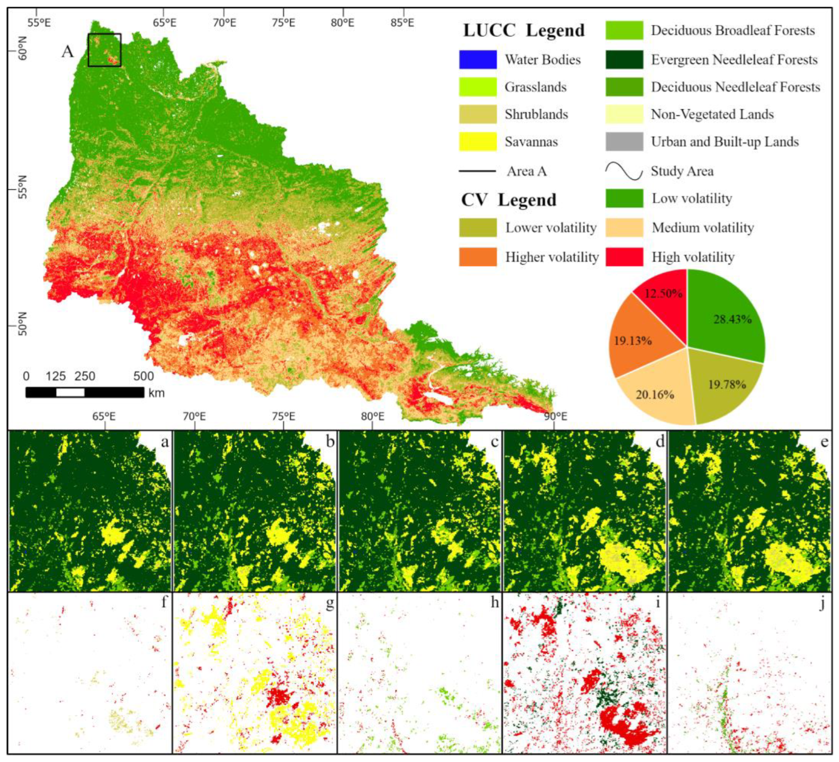

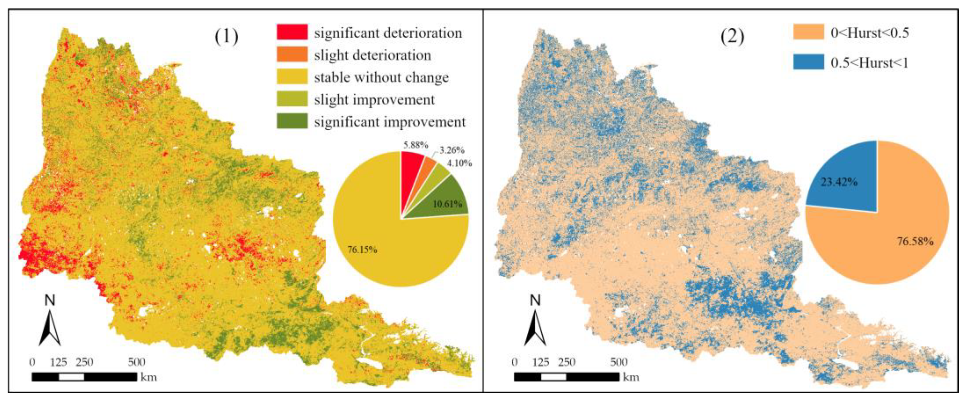

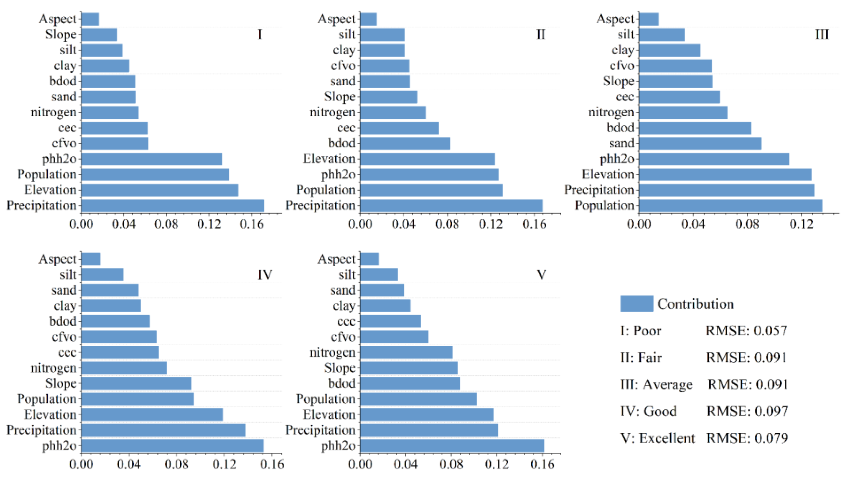
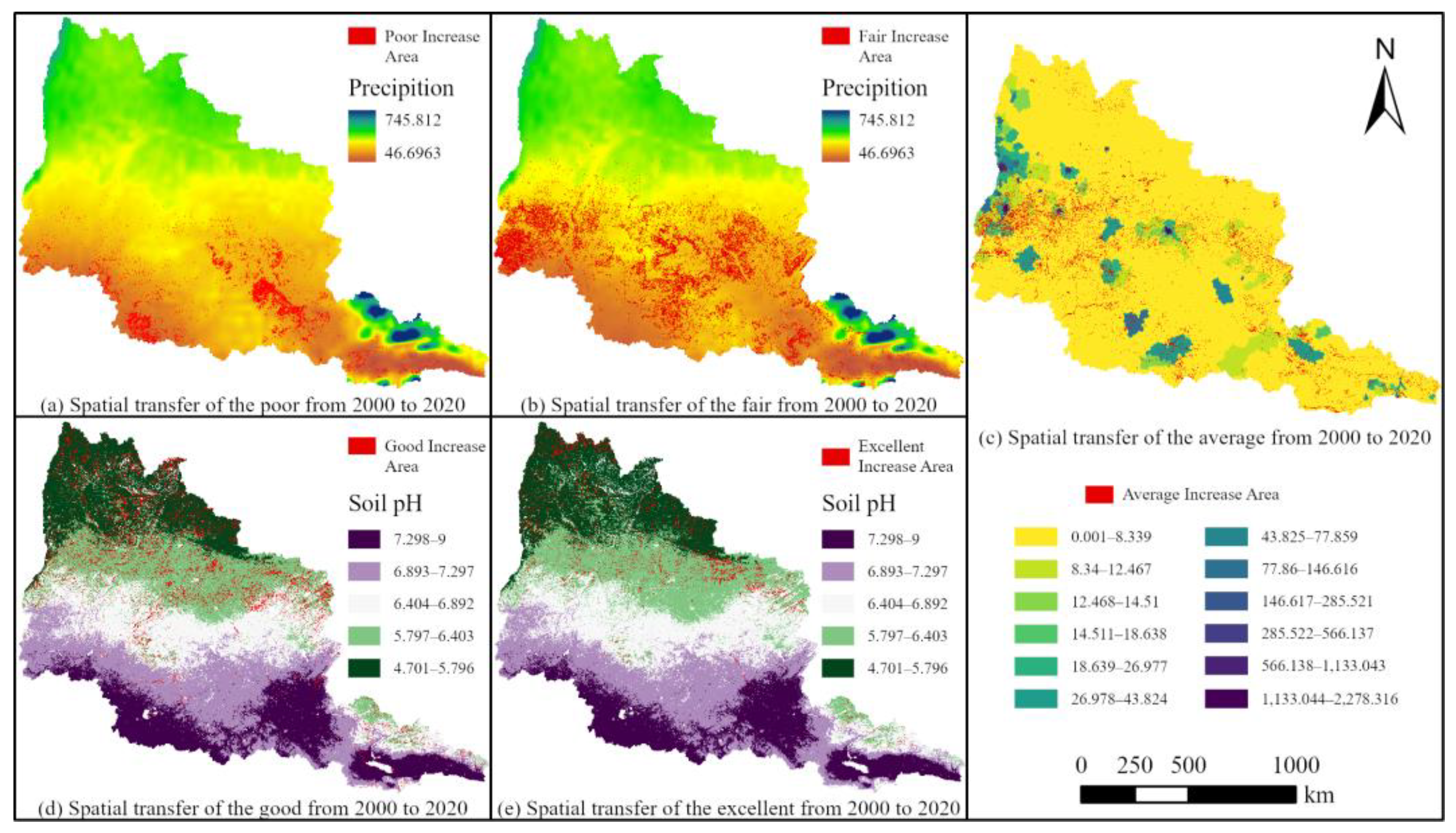
Disclaimer/Publisher’s Note: The statements, opinions and data contained in all publications are solely those of the individual author(s) and contributor(s) and not of MDPI and/or the editor(s). MDPI and/or the editor(s) disclaim responsibility for any injury to people or property resulting from any ideas, methods, instructions or products referred to in the content. |
© 2024 by the authors. Licensee MDPI, Basel, Switzerland. This article is an open access article distributed under the terms and conditions of the Creative Commons Attribution (CC BY) license (https://creativecommons.org/licenses/by/4.0/).