Downscaling Global Land-Use Scenario Data to the National Level: A Case Study for Belgium

Abstract

Land use change scenarios, and their projected impacts on biodiversity, are highly relevant at local scales but not adequately captured by the coarse spatial resolutions of global land use models. In this study, we used the land use allocation tool of the GLOBIO 4 model to downscale the Land Use Harmonization v2 (LUH2) data from their original spatial resolution (0.25°) to 100 m and 10 m resolutions, using the country of Belgium as an example. Inputs to the tool included: (1) a reference present-day land cover map at the high spatial resolution, (2) regional land demand projections for three future scenarios, Sustainability (SSP1xRCP2.6), Regional Rivalry (SSP3xRCP6.0), and Fossil-fuelled Development (SSP5xRCP8.5), and (3) raster layers representing the suitability of the grid cells for different land use types. We further investigated the impact of using different reference land cover maps (CORINE at 100 m resolution and ESA WorldCover at 100 m and 10 m resolutions) on the downscaling outcomes. Comparison of downscaled current and future land use maps with the original LUH2 dataset showed that the use of ESA WorldCover as a reference map provides better agreement (RSR: 0.11–0.24, overall accuracy: 0.94–0.98, Kappa: 0.91–0.97) than CORINE (RSR: 0.28–0.33, overall accuracy: 0.90–0.93, Kappa: 0.90–0.91). Additionally, the validation of the present-day downscaled maps showed a good agreement with the independent Copernicus Global Land Service dataset. Our findings suggest that the choice of reference land cover map influences the degree of agreement between the downscaled and the original coarse-grain land-use maps. Moreover, the land use maps produced using our downscaling approach can provide valuable insights into the potential impacts of land use change on biodiversity and can guide local decision-making processes for sustainable land management and conservation efforts.

1. Introduction

Land use and land cover (LULC) change has been the primary cause of the global loss of terrestrial biodiversity over the past century and is likely to remain a key driver for future changes [1,2,3]. Land use change will also interact with the impacts of climate change on biodiversity and ecosystem services [4]. For example, land use changes may impair the ability of species to shift their distributions in response to climate change [5]. Land use and climate change also jointly affect ecosystem services like erosion control, where land use change and management may either counteract or reinforce the increased risks of landslides due to climate change [6,7,8]. Similarly, climate change is expected to disrupt hydrological processes, which might be exacerbated by land use change [9]. These studies underscore the significance of proactive land use planning and climate change mitigation for sustainable natural resource management and for safeguarding biodiversity and ecosystem services [1].

The Intergovernmental Panel on Climate Change (IPCC) has encouraged the development of global scenarios to inform climate mitigation and adaptation strategies [10]. The Representative Concentration Pathways (RCPs) represent various climate futures based on alternative greenhouse gas emission trajectories over the 21st century [11]. These emissions pathways have been integrated into climate projections in the most recent phase of the Coupled Model Intercomparison Project (CMIP6) [10]. In parallel, the climate research community has created several Shared Socioeconomic Pathways (SSPs), representing future societal development paths with various socioeconomic conditions and associated land-use projections [12,13]. The SSPs can be paired with RCP-based climate projections to investigate a variety of possibilities for climate and land use change, and they are being utilised in a wide variety of impact modeling efforts and intercomparisons [14,15,16]. The Intergovernmental Science-Policy Platform on Biodiversity and Ecosystem Services (IPBES) has advised utilising the SSP-RCP framework to simulate the consequences on biodiversity and ecosystem services since it offers a great opportunity to build bridges between the climate, biodiversity, and ecosystem services communities [10].

Land Use Harmonisation v2 (LUH2) is a harmonised dataset of future land use projections created in line with the SSP-RCP framework [17]. It was released for the preparation of the IPCC Sixth Assessment Report (AR6) and as part of CMIP6 [18]. LUH2 offers a harmonised set of land-use scenarios that smoothly connects historical land-use reconstructions with eight future projections in the format required for Earth System Models (ESM) [17]. Various studies have explored biodiversity and ecosystem service changes using the LUH2 data [2,3,10]. However, the LUH2 dataset has a spatial resolution of 0.25°, which is too coarse to meet the needs of local scale research and decision-making [17,18] and tends to underestimate the spatial heterogeneity of land-use patterns [19]. For instance, Li et al. [20] showed that land use products with a coarse resolution underestimate the amount of urban land use change and do not adequately capture the spatial patterns of urbanisation and its impact on local or regional climate. Similarly, Schaldach et al. [21] highlight the limitations of the 5 arc-minute resolution global land product in capturing fine-scale processes such as carbon sequestration. Hence, a set of higher-resolution land use projections under different future scenarios are needed for localised LULC projections, which is vital for improving impact assessments to inform management and support decision-making [18]. For example, high-resolution LULC projections may help to inform watershed assessments, species distribution modeling, habitat mapping, and ecosystem services evaluation [22,23].

Several studies have tried to downscale relatively coarse grain land use projections to a higher spatial resolution. For example, Giuliani et al. [24] focused on the development of high-resolution and detailed LULC maps for Switzerland. They used a combination of the Swiss topographic base map and national LULC statistics obtained from aerial photo interpretation to generate downscaled maps for three time periods. The spatial resolution increased from 100 m to 25 m, and the number of land use categories increased from 29 to 62. The method involved spatial weighting and expert system-based correspondence to ensure accurate mapping. Hoskins et al. [19] implemented a statistical model for downscaling the LUH2 data to provide global estimates at 30 arc-seconds (1 km) resolution for five land use classes. To our knowledge, Schipper et al. [3] achieved the highest spatial resolution for global land use projections by downscaling the LUH2 data to a 10 arc-seconds (300 m) resolution using the Global biodiversity model for policy support (GLOBIO). However, their study did not explore how local and national land use responds to global mitigation policies, and their spatial resolution was not sufficiently fine for supporting local environmental adaptation and decision-making.

In this study, we aimed to address these limitations by exploring the potential of GLOBIO’s land use allocation model to downscale land use information to finer spatial resolutions of 100 m and 10 m, using the country of Belgium as a case study. Our specific objective was to analyze how the choice of reference land cover map, which is one of the key inputs for GLOBIO’s land allocation model, affects the result of the downscaling process. Specifically, we compare three reference maps: the 10 m resolution European Space Agency (ESA) WorldCover map, the WorldCover map resampled to a 100 m resolution, and the pan-European CORINE land cover map at a 100 m resolution. We then use these background maps as input to the land allocation module for downscaling coarse-grain land use data for both the present and three future development pathways. Following the biodiversity model intercomparison protocol [10], we used three different pairings of SSPs and RCPs to ensure the combinations encompass a broad range of future land use and climate change scenarios. Specifically, in the Sustainability scenario, SSP1 (moderate land use pressure) was linked with the RCP2.6 (low level of climate change) pathway. In the Regional Rivalry scenario, SSP3 (high land use pressure) was linked with the RCP6.0 (moderate level of climate change) pathway. Lastly, in the Fossil-fueled Development scenario, SSP5 (moderate land use pressure) was connected to the RCP8.5 (high level of climate change) pathway. The SSP3xRCP6.0 and SSP5xRCP8.5 combinations represent scenarios with minor or no climate change mitigation policies. Our study provides novel methodological insights relevant to downscaling land-use projections as well as an example of deriving land-use projections at spatial resolutions of greater ecological relevance than has been possible before.

2. Materials and Methods

2.1. Case Study Area

Our case study area is the country of Belgium, which is a small and highly urbanised country in the densely populated region of Western Europe with an average population density of circa 370 inhabitants per km², as per the 2018 data [25,26]. Belgium was chosen as a case study because of its diversified land use patterns, environmental variability, and good data availability [25], making it an ideal country for downscaling land use data and advancing our understanding of land use dynamics at the local scale. Belgium, despite its small size, contains a lot of geographical variation. The Baltic Plain is to the north, while the old Hercynian massifs of Central Europe lie to the south. Apart from the Ardennes region in the southwest, the climate is warm and moist, allowing for extensive grass growth. Arable farming is most prevalent in the central part of the country. Because most of the country’s southern region (particularly the Hautes–Ardennes) has a harsh climate and soils that prevent the development of arable crops, grasslands and forests are the major land uses [2,27,28].

2.2. LUH2 Data

The Land Use Harmonisation dataset version 2 (LUH2) is a global time series of past, present, and future land use at 0.25°, spanning 850–2300 [17]. It includes estimates of historical land-use change (850–2015) and future projections (2015–2300) that were generated by integrating and harmonising land-use history with future projections from various integrative assessment models (IAMs) [10,28,29,30]. The dataset describes the proportional cover in each 0.25° grid cell of twelve land-use categories: forested primary land (primf), non-forested primary land (primn), potentially forested secondary land (secdf), potentially non-forested secondary land (secdn), managed pasture (pastr), rangeland (range), urban land (urban), c3 annual crops (c3ann), c3 perennial crops (c3per), c4 annual crops (c4ann), c4 perennial crops (c4per), c3 nitrogen-fixing crops (c3nfx). LUH2 has a greater spatial resolution than the first-generation LUH1 (0.25° vs. 0.50°), and more detailed land-use transitions (12 vs. 5 potential land-use classes) [17]. With annual time steps, LUH2 supports over 100 possible transitions per grid cell per year (e.g., crop rotations, shifting cultivation, agricultural changes, wood harvest) and numerous agricultural management layers (e.g., irrigation, synthetic nitrogen fertilizer, biofuel crops) [10,17]. Primary and secondary natural vegetation are divided into forest and non-forest sub-types, pasture is divided into managed pasture and rangeland, and cropland is divided into multiple crop functional types (C3 annual, C3 perennial, C4 annual, C4 perennial, and N fixing crops) [10]. We selected this dataset for two reasons: (1) it is the most complete data in terms of time-series and scenarios of climate change [17] and offers a new harmonised set of land-use scenarios that smoothly connects historical land-use reconstructions with eight future projections, and (2) it has been used widely by IPBES in support of its global and regional assessments of biodiversity and ecosystem service change [31].

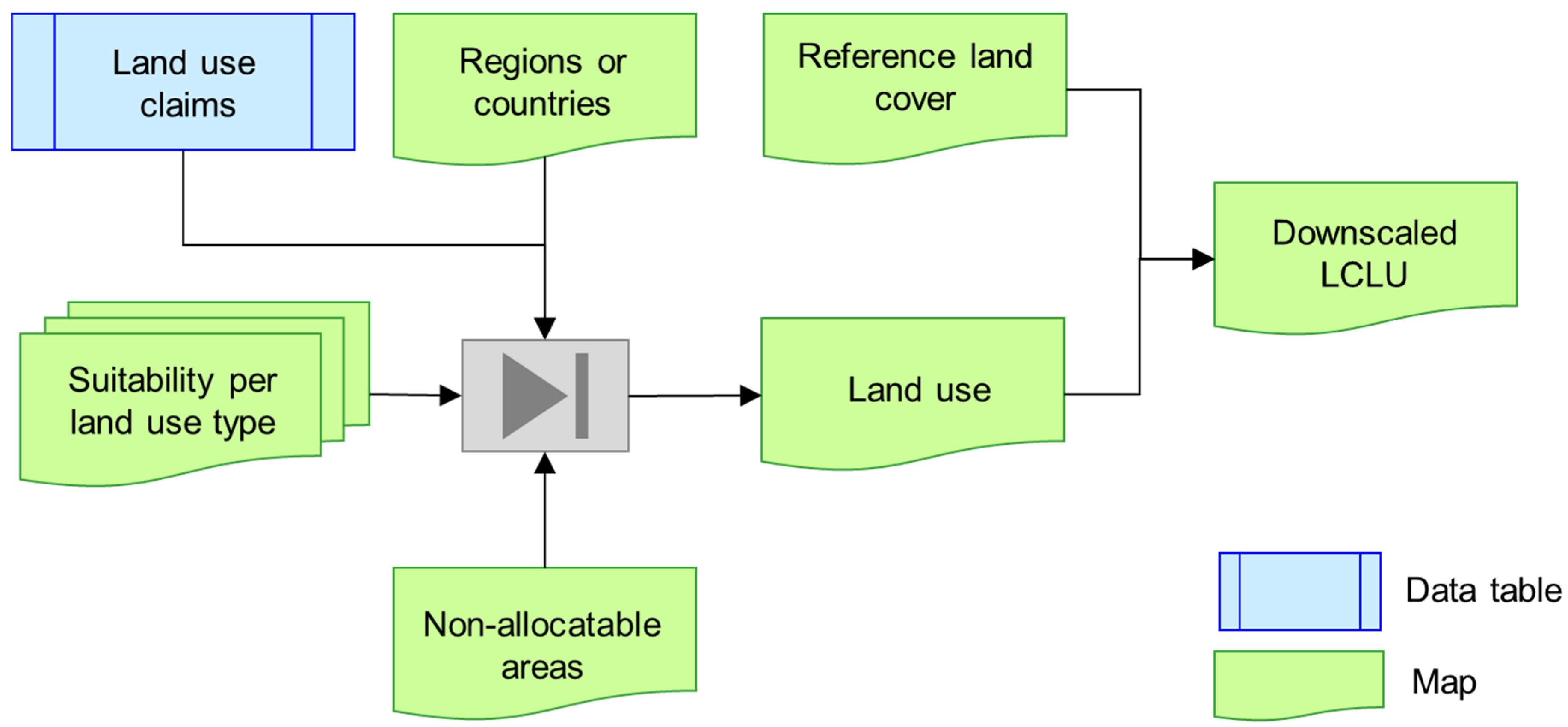
2.3. GLOBIO Land-Use Downscaling Tool

We downscaled the LUH2 data with the land-use downscaling module included in the GLOBIO modelling framework [3]. The GLOBIO model is hosted and maintained by PBL Netherlands Environmental Assessment Agency and is intended to inform and support policymakers by quantifying global human impacts on biodiversity and ecosystems [3,32]. The current version of the GLOBIO model, version 4, includes a land-use allocation module capable of downscaling (or spatially allocating) low-resolution land use data (regional totals or ‘claims’) to a high-resolution discrete land use map. The allocation algorithm can use user-defined land use classes and their corresponding regional totals, or “claims”, represented in surface area per region per land-use class. The regional totals of each land use class are spatially allocated based on an overall ‘suitability layer’ for that class (Figure 1). Claims can be obtained from national or regional statistics or from IAMs that estimate land demand based on socioeconomic development [3] and must be expressed as area (km²). The allocation algorithm prioritizes candidate grid cells according to their suitability values and allocates the claims of each land use type in each region, starting from the cells with the highest suitability, until the total claim is allocated. During allocation, a predefined order is followed, where urban land takes precedence over cropland [33] and cropland, in turn, takes precedence over pasture [34]. If multiple cells have the same suitability, the allocation is conducted randomly. Forestry and pasture are allocated thereafter, such that forestry is allocated within remaining forest areas, and grazing typically takes place in areas not productive enough for crops [34]. The cells that are not allocated to any land use class are assigned the land cover type retrieved from a so-called background map [3]. If the land claim allocated in a given scenario–year is smaller than the claim allocated in the preceding scenario–year, the least suitable cells are abandoned and assigned to secondary vegetation. As inputs, the downscaling module requires a layer with the boundaries of the region (s), a reference land cover map at the desired spatial resolution (10 m and 100 m in our case), map layers quantifying the suitability of each grid cell for each land-use type and a map of non-allocatable areas, each also at the desired resolution, and the areas (‘claims’) of each land use type (Figure 1).

2.4. Input Data Preparation

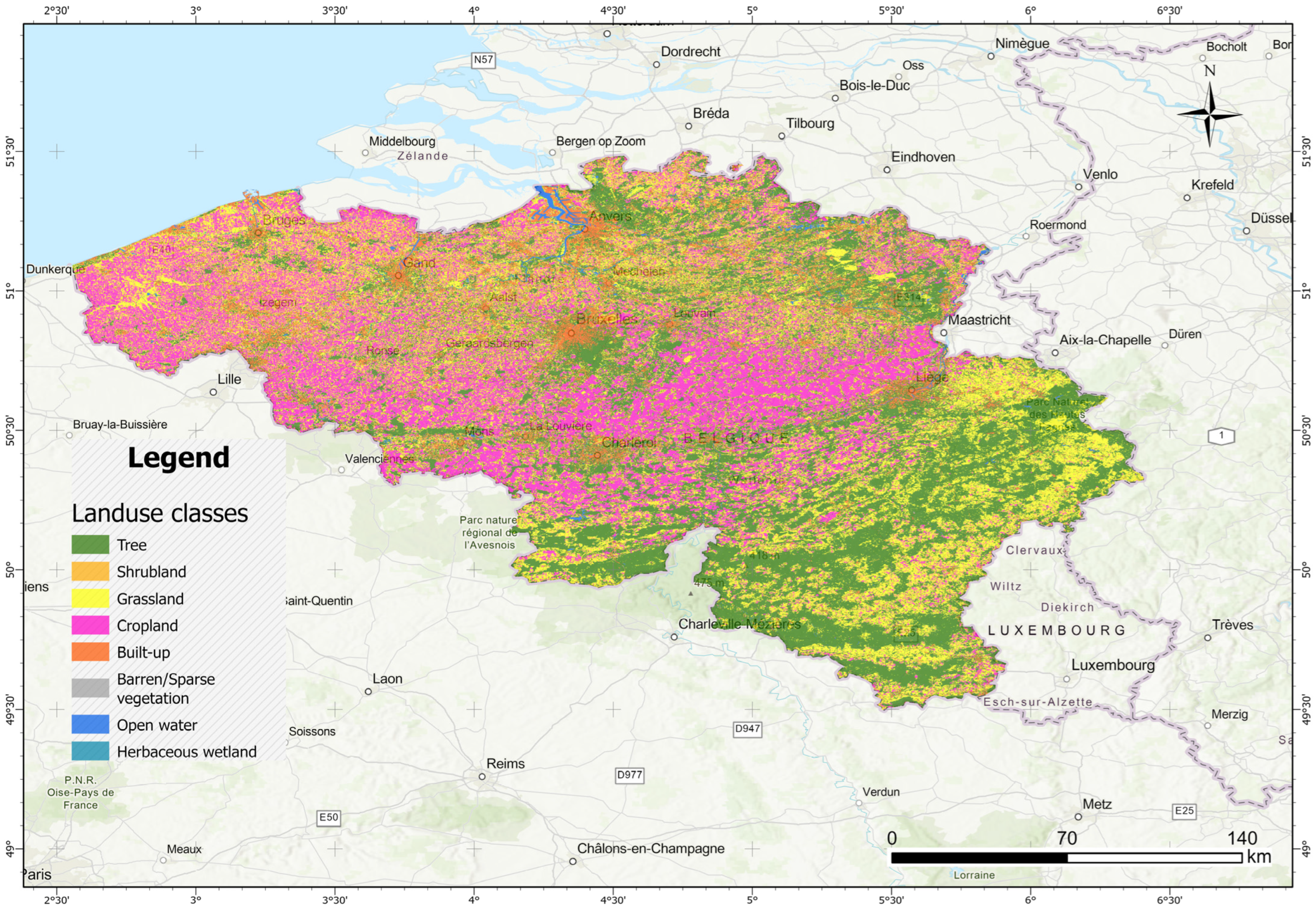
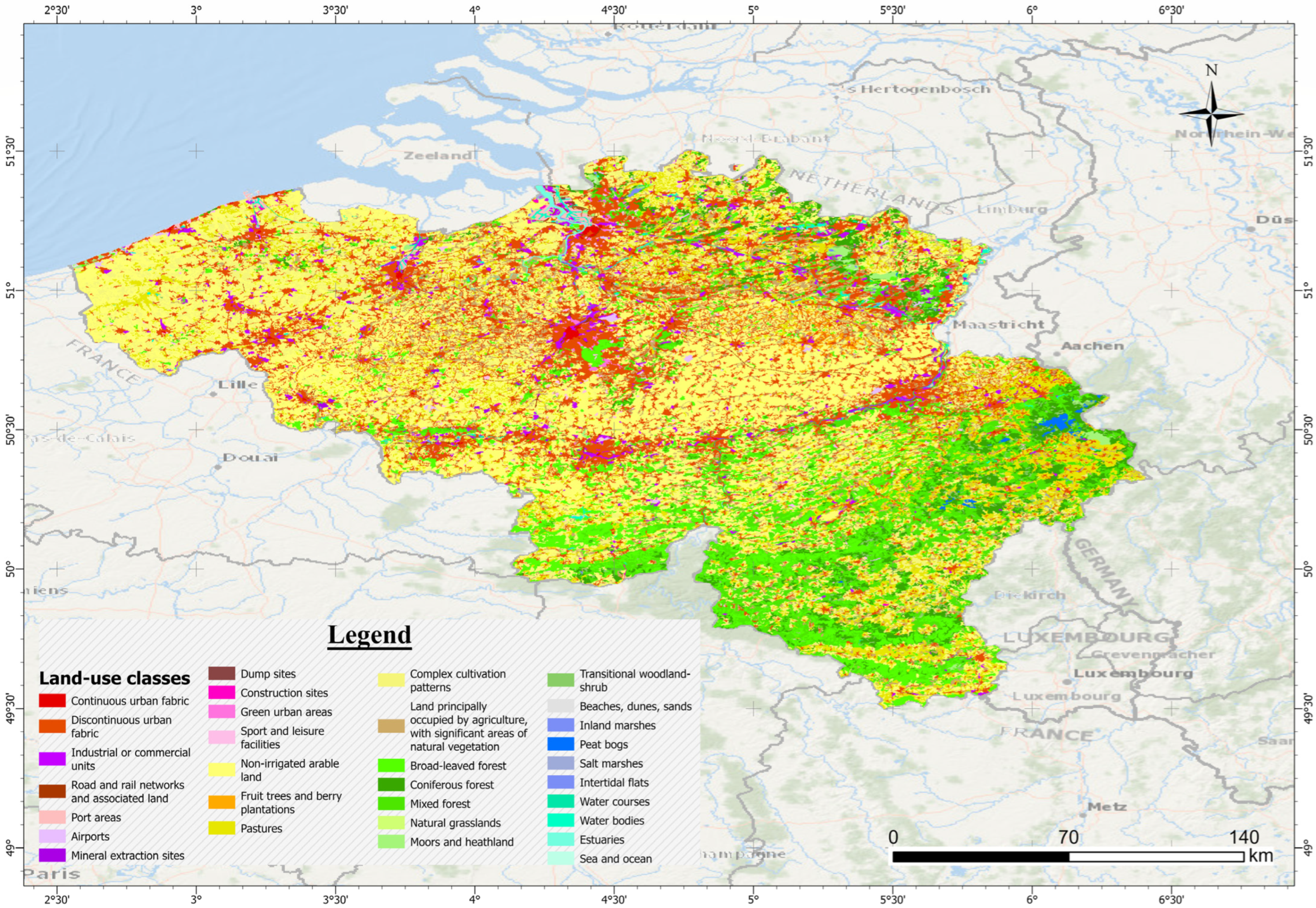
2.4.1. Reference Land Cover Maps

For the downscaling of the LUH2 dataset, we employed three different background maps to guide the spatial downscaling process, which enabled us to compare the impact of the source and spatial resolution of the reference map on the result. At the highest resolution (10 m), we used the European Space Agency (ESA) WorldCover map for the year 2020 [35]. This product provides a global land cover map at 10 m resolution based on Sentinel-1 and Sentinel-2 satellite data. The classification system of ESA WorldCover is different from LUH2, with 12 land use classes in the LUH2 datasets and 11 land use classes in ESA WorldCover (

Table 1. Overview of LULC classes in LUH2, CORINE, and ESA WorldCover and their reclassification in the downscaled land-use maps.

LUH2	CORINE	ESA WorldCover	Downscaled Map
Urban land	Continuous urban fabric Discontinuous urban fabric Industrial or commercial units Road and rail networks and associated land Port areas Airports Mineral extraction sites Dump site Construction sites Green urban areas Sport and leisure facilities	Built-up	Urban
C3 annual crop C3 perennial crop C4 annual crop C4 perennial crop C3 nitrogen-fixing crop Non-irrigated arable land Fruit trees and berry plantations Complex cultivation patterns Land principally occupied by agriculture, with significant areas of natural vegetation	Non-irrigated arable land Fruit trees and berry plantations Complex cultivation patterns Land principally occupied by agriculture, with significant areas of natural vegetation	Cropland	Cropland
Managed pasture Rangeland	Pasture	NA	Pasture
Forested primary land Potentially forested secondary land Non-forested primary land Potentially non-forested secondary land	Broad-leaved forest Coniferous forest Mixed forest Moors and heathland Transitional woodland-shrub Natural grasslands Beaches, dunes, sands	Tree cover Shrubland Grassland Bare/sparse vegetation	Natural
NA	Glaciers and perpetual snow Inland marshes Peat bogs Salt marshes Intertidal flats Water courses Water bodies Estuaries Sea and ocean	Open water Herbaceous wetland	Not allocatable

and Figure 2). At a 100 m resolution, we used the Coordination of Information on the Environment (CORINE) Land Cover 2018 data as the reference map. The classification system of CORINE is more detailed compared to LUH2, with 12 land use classes in the LUH2 datasets and 44 land use classes in CORINE (Table 1 and Figure 3). We obtained a third reference map by upscaling the ESA WorldCover map to 100 m, which is the same resolution as the CORINE land cover map. In our upscaling process, we employed the majority rule approach. This means that we assigned to each larger cell the value of the most prevalent LULC class from the smaller cells within it, thus capturing the dominant LULC class.

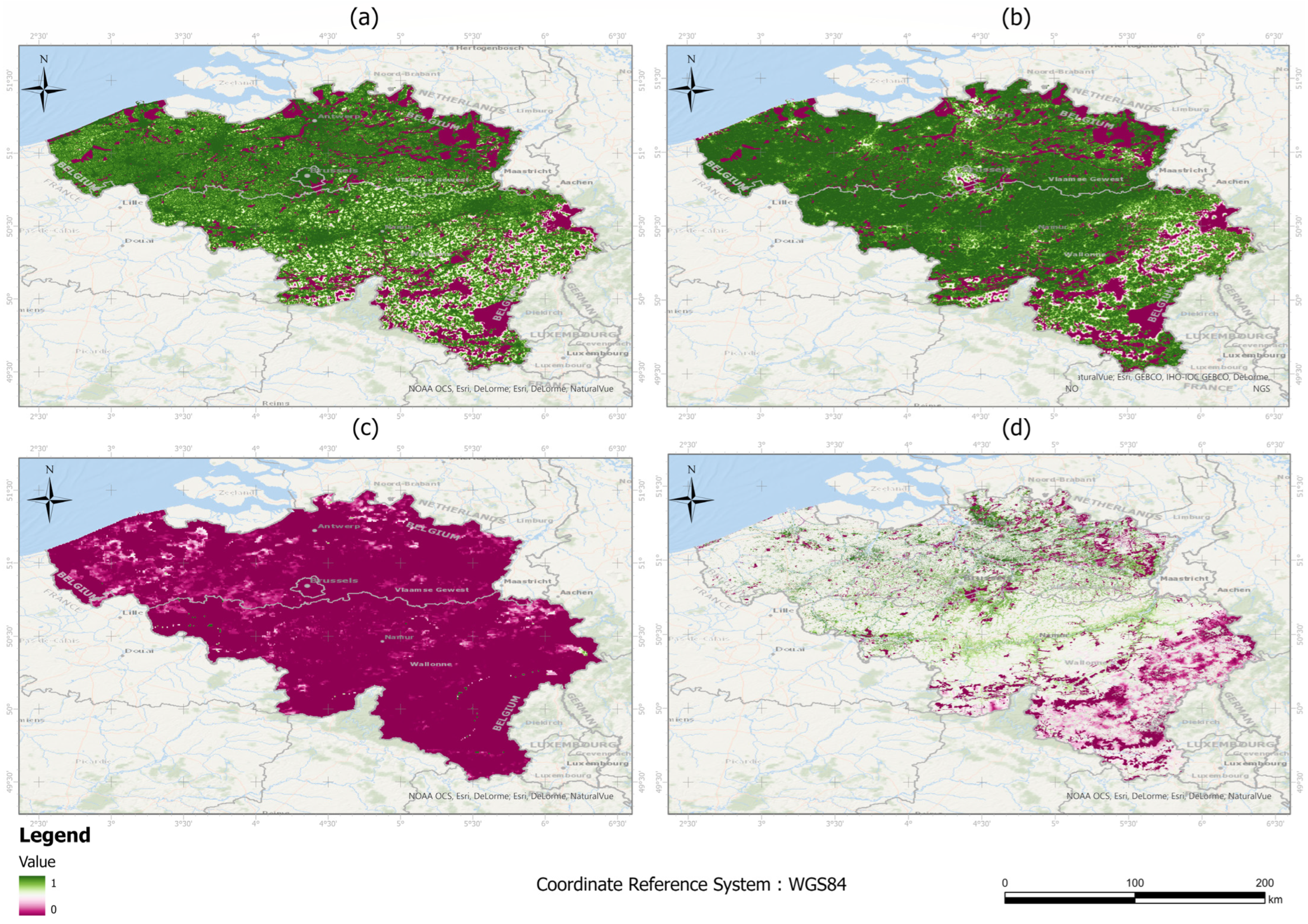
2.4.2. Suitability Layers

For each of the three reference maps, we created suitability layers for four major land-use types (urban area, cropland, pasture, and forestry; see Figure 4), following the approach described by Schipper et al. [3]. Because spatial clustering and edge expansion have been identified as significant factors in the growth of urban areas and croplands, we retrieved the suitability layers for urban areas and croplands based on their proximity to existing urban areas and croplands [36,37,38]. To that end, we first used the reclassified reference land cover maps to calculate the Euclidean distance to existing urban areas or croplands, assigned the highest suitability to existing cropland or urban area, and inverted and normalised the distances to existing urban areas or cropland. We also set the suitability of non-urban and non-cropland cells inside protected areas to zero based on the assumption that urban and cropland areas within protected areas would not expand beyond what they were in 2020 [3]. The World Database of Protected Areas (WDPA) was used to identify the protected areas [3].

We created a pasture suitability layer based on the density of ruminant livestock species (goats, sheep, and cattle) from the Food and Agriculture Organization (FAO)’s gridded livestock of the world dataset (GLW; head per km², 30 arc-seconds) [39]. Modelled livestock densities are provided by the GLW, which are based on detailed subnational livestock statistics and a set of predictor variables linked to climate, vegetation, topography, and demography. To account for variances in body mass among livestock species, we converted their densities to tropical livestock units [40] summed the units per grid and normalised to achieve suitability values ranging from 0 to 1.

We assumed that access to wood is mostly determined by elevation, proximity to infrastructure, and the presence of protected areas [3]. We calculated the Euclidean distance to the nearest road using road data from the Global Roads Inventory Project (GRIP) database [41]. To obtain suitable values between 0 and 1, we inverted and normalised the distances and multiplied the resulting values with inverted and normalised elevation values (retrieved from the Copernicus Land Monitoring Service). We also assumed that no forestry activities would take place in protected areas. Therefore, we set the suitability values for forestry inside protected areas to zero. Finally, we clipped the forestry suitability layer to the land cover with trees and set the suitability of other cells to zero [3].

2.4.3. Claims

We obtained claims of urban area, cropland, pasture, and forestry as the country-level total areas of each type for each scenario-year. For the present-day situation (baseline year 2015), we obtained urban area and cropland claims from the respective land cover background maps (i.e., ESA WorldCover 2020, its 100 m resolution upscaled version, and the 100 m CORINE map). Similarly, for downscaling pasture based on the CORINE reference map we obtained present-day pasture claims from the same map. For the land use classes that cannot be distinguished from natural land cover (pasture and forestry in ESA WorldCover and forestry in CORINE), we obtained claims using FAO’s country-level statistics for 2018 (for CORINE) or 2020 (for WorldCover). We defined the pasture claim as the sum of all country-level permanent and temporary meadows and the forestry claim as the sum of all country-level planted trees [3]. To estimate the claims for the future land-use maps, we used the original LUH2 dataset to calculate the change in country-level total areas of the four land-use types (urban, farmland, pasture, and forestry) between 2015 and 2050, for each of the three SSP scenarios (

Table 2. Total area (km²) of different land use types per scenario and changes (%) in the area relative to 2015 based on the LUH2 dataset.

Land Use Type	2015	Sustainability Scenario		Regional Rivalry Scenario		Fossil-Fuelled Development Scenario
	Area (km2)	Area (km2)	Change (%)	Area (km2)	Change (%)	Area (km2)	Change (%)
Urban	3134	3635	16	3346	6	4011	28
Cropland	8601	7227	−16	10,866	26	8813	2
Pasture	5886	3137	−47	4781	−18	5886	0
Forestry	4609	5431	18	3980	−6	4375	−5

). We chose 2015 as the present-day estimate because the historical land-use forcing dataset from LUH2 is until 2015. We calculated cropland claims as the sum of the areas of the five cropland types included in LUH2 (c3ann + c3per + c4ann + c4per + c3nfx), forestry claims as the sum of wood harvest from forested cells and non-forested cells with primary and secondary vegetation (primf harv + primn harv + secdf harv + secdn harv), and pasture claims as the sum of pasture and rangeland areas (Table 2). For each future scenario year, we calculated the difference in the area of each land use type relative to 2015 (LUH2 historical dataset) and added the difference to the present-day claims (as mentioned above), with the result being the overall claim for 2050 [3]. Thus, rather than defining the claims themselves, we used the LUH2 data to define the change in claims. Our rationale was that the integrated assessment models underlying LUH2 are good at representing temporal trends in land use. However, remote sensing data and national statistics, included in our present-day land-use map, better represent the current situation [3].

2.4.4. Non-Allocatable Areas

Areas that are expected to undergo no land use expansion are referred to as non-allocatable areas (Table 1). A map with non-allocatable areas was constructed by dividing the reference land cover maps into two classes: non-allocatable areas (wetlands and water; Table 1) and allocatable areas (everything else).

2.5. Evaluation and Validation of the Downscaled Maps

After downscaling, we reclassified the resulting maps in order to facilitate comparison with the original LUH2 data (see Table 1). The downscaled and reclassified maps include the four major anthropogenic land-use classes and secondary vegetation. The class “secondary vegetation” originates when anthropogenic classes that existed in 2015 are abandoned in 2050 due to a decline in demand. Further, we reclassified all the natural land-cover classes, such as natural forest and natural grassland, into a single category labeled “natural”.

We conducted two accuracy assessments of our downscaled and reclassified land-use maps. First, we determined how well our downscaled product matched the original LUH2 data. This evaluation covered both current and future scenarios. Next, to validate the accuracy of the present-day downscaled maps, we assessed their degree of agreement with the independent Copernicus Global Land Service dataset for the year 2015, which has a spatial resolution of 100 m [42]. This validation was restricted to the urban and cropping layers because the Copernicus Global Land Service dataset does not include forestry and pasture as distinct land classes. To evaluate the agreement in the spatial patterns, we used the overall accuracy and the Kappa coefficient, which are commonly used measures for assessing the accuracy of a LULC map [43,44,45,46,47]. The overall accuracy (Ô) calculates the proportion of correctly classified cells relative to the total number of pixels (Equation (1)):

$$Ô=\frac{\sum _{\mathrm{i}=1}^{\mathrm{r}}{\mathrm{n}}_{\mathrm{i}\mathrm{j}}}{\mathrm{N}}$$

(1)

where:

• n_ij represents the number of correctly classified pixels for class i
• N is the total number of pixels
• r = the number of the classes

The Kappa coefficient (K) is computed based on the error matrix and quantifies the level of agreement between two categorical datasets [48], as (Equation (2)):

$$\mathsf{{\rm K}}=\frac{\mathsf{{\rm N}}{\sum }_{\mathfrak{i}=1}^{\mathrm{r}}{\mathsf{{\rm X}}}_{\mathfrak{i}\mathfrak{i}}-{\sum }_{\mathfrak{i}=1}^{\mathrm{n}}{({\mathsf{{\rm X}}}_{\mathfrak{i}+}·\mathsf{{\rm X}}}_{+\mathfrak{i}})}{{\mathrm{N}}^2-{\sum }_{\mathfrak{i}=1}^{\mathrm{n}}{({\mathsf{{\rm X}}}_{\mathfrak{i}+}·\mathsf{{\rm X}}}_{+\mathfrak{i}})}$$

(2)

where:

• ${\mathsf{{\rm X}}}_{\mathfrak{i}\mathfrak{i}}$ is the number of pixels that are correctly classified
• ${\mathsf{{\rm X}}}_{\mathfrak{i}+}$ represents the number of pixels in a downscaled map
• ${\mathsf{{\rm X}}}_{+\mathfrak{i}}$represents the number of pixels in a reference data
• N is the total number of pixels
• r = the number of classes
• i = the i th class

A K value of 1 represents a perfect agreement, while a value of 0 represents no agreement.

Further, we calculated the Root Mean Squared Error—observations standard deviation ratio (RSR) between the total areas of the land use types in the downscaled maps and the original LUH2 data (for cropland, urban, forestry, and pasture) and the Copernicus Global Land Service data (for urban and cropland). The RSR is a well-established error index [49] and is calculated as (Equation (3)):

$$\mathrm{R}\mathrm{S}\mathrm{R}=\frac{\mathrm{R}\mathrm{M}\mathrm{S}\mathrm{E}}{{\mathrm{S}\mathrm{T}\mathrm{D}\mathrm{E}\mathrm{V}}_{\mathrm{O}\mathrm{B}\mathrm{S}}}= \frac{\left[\sqrt{\sum _{\mathrm{i}=1}^{\mathrm{r}}{({\mathrm{Y}}_{\mathrm{i}}^{\mathrm{o}\mathrm{b}\mathrm{s}}-{\mathrm{Y}}_{\mathrm{i}}^{\mathrm{p}\mathrm{r}\mathrm{e}\mathrm{d}})}^2}\right]}{\left[\sqrt{\sum _{\mathrm{i}=1}^{\mathrm{r}}{({\mathrm{Y}}_{\mathrm{i}}^{\mathrm{o}\mathrm{b}\mathrm{s}}-{\mathrm{Y}}_{\mathrm{i}}^{\mathrm{m}\mathrm{e}\mathrm{a}\mathrm{n}})}^2}\right]}$$

(3)

where:

• r: Total number of observations
• ${\mathrm{Y}}_{\mathrm{i}}^{\mathrm{o}\mathrm{b}\mathrm{s}}$: Actual observed value for the i-th observation
• ${\mathrm{Y}}_{\mathrm{i}}^{\mathrm{p}\mathrm{r}\mathrm{e}\mathrm{d}}$: Value predicted by the model for the i-th observation
• ${\mathrm{Y}}_{\mathrm{i}}^{\mathrm{m}\mathrm{e}\mathrm{a}\mathrm{n}}$: Calculated mean of the observed values
• ${\mathrm{S}\mathrm{T}\mathrm{D}\mathrm{E}\mathrm{V}}_{\mathrm{O}\mathrm{B}\mathrm{S}}$: standard deviation of observed data

This formula calculates the RSR by first computing the Root Mean Squared Error (RMSE), which measures the average magnitude of differences between predicted (${\mathrm{Y}}_{\mathrm{i}}^{\mathrm{p}\mathrm{r}\mathrm{e}\mathrm{d}}$) and observed (${\mathrm{Y}}_{\mathrm{i}}^{\mathrm{o}\mathrm{b}\mathrm{s}}$) values. Then, it divides the RMSE by the standard deviation of observed values (using squared differences from the mean) to normalize the model’s predictive accuracy based on the inherent variability in the observed data. Thus, RSR offers a standardised measure to assess the alignment of model simulations with observed data, considering the variability of the observed data. The RSR value ranges from 0, indicating perfect model simulation with zero RMSE or residual variation, to a large positive number. Generally, a lower RSR indicates better model performance [49].

3. Results

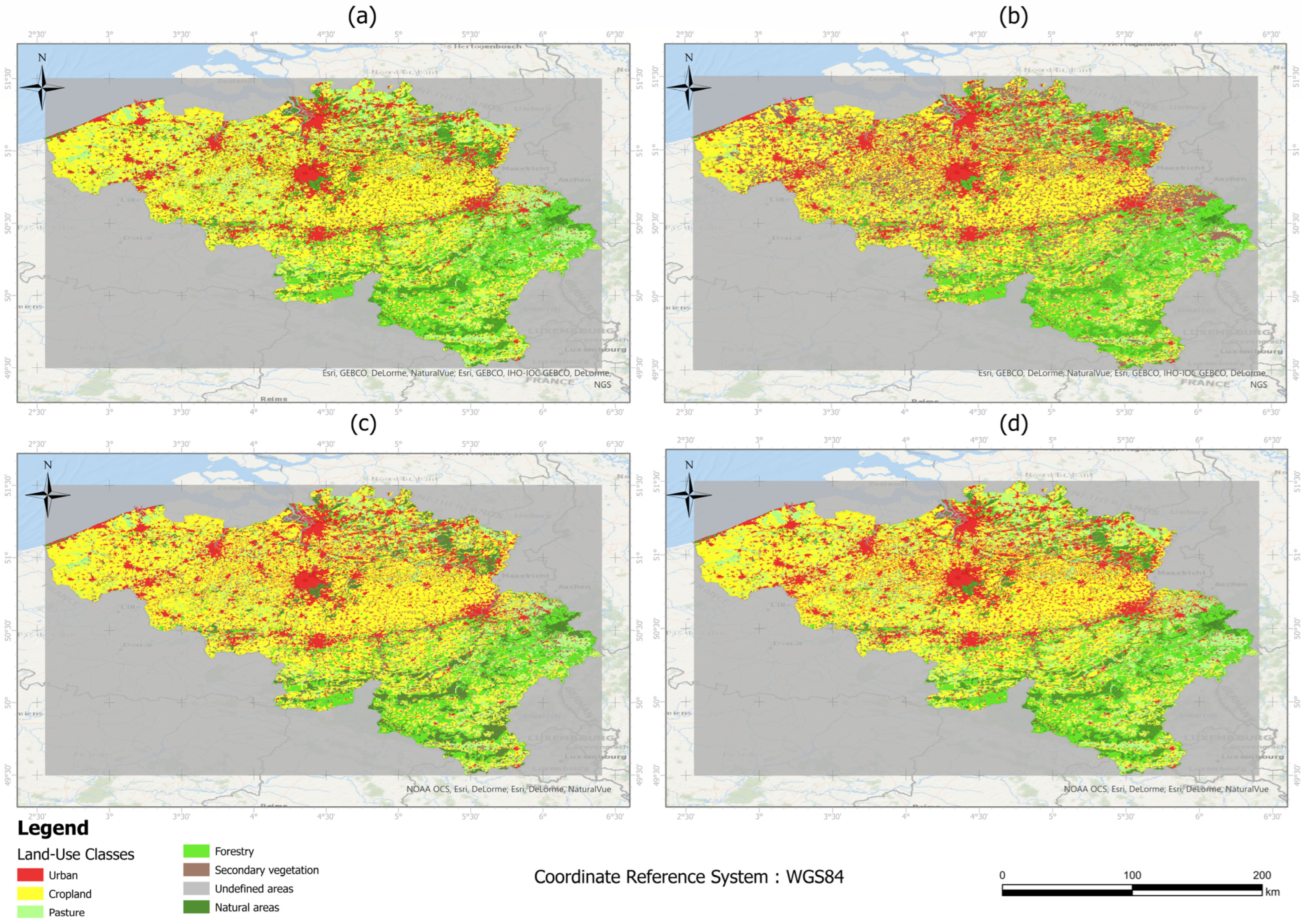
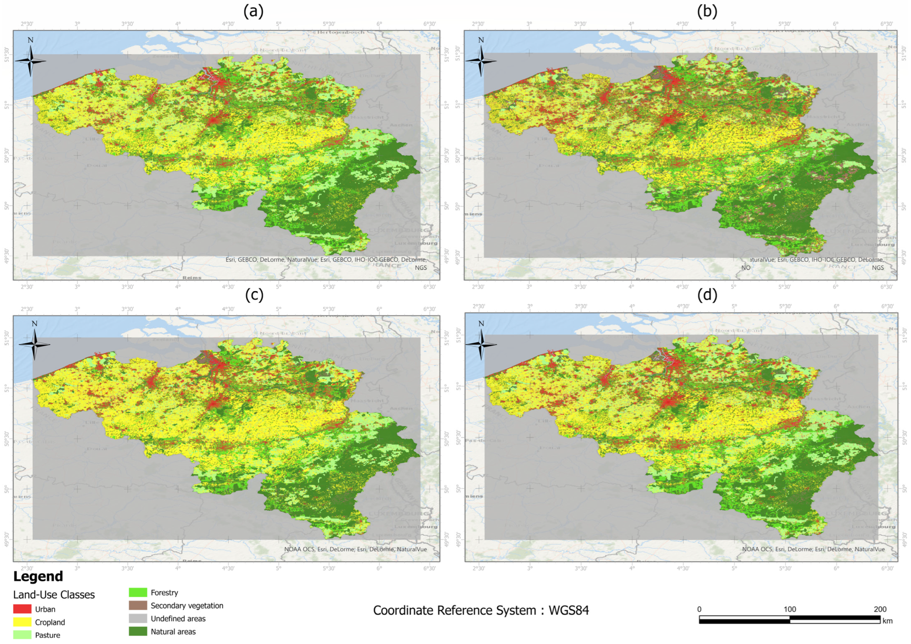
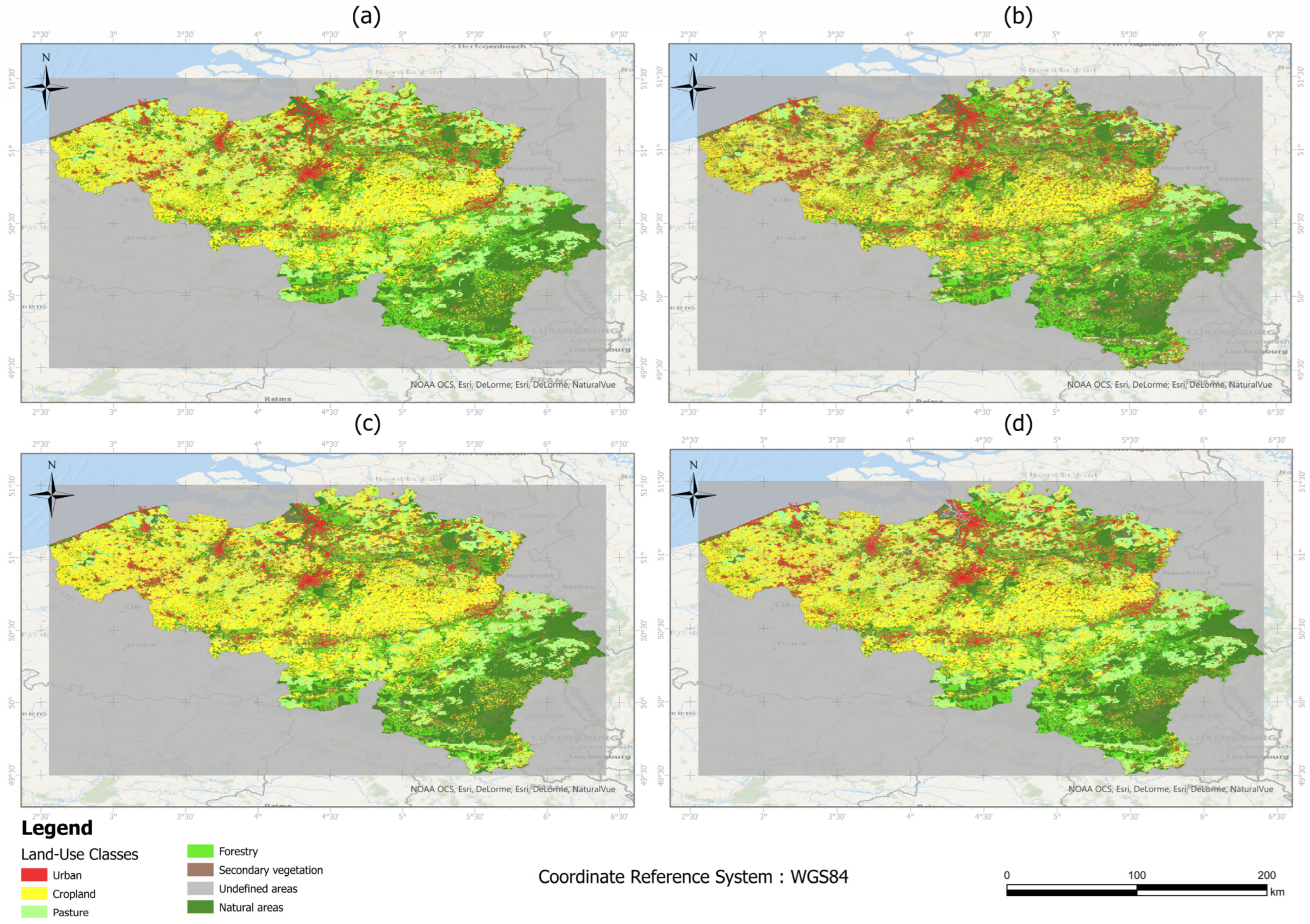
3.1. Downscaled Land-Use Maps

The downscaled land-use maps at 10 m and 100 m show roughly similar patterns in major LULC types (Figure 5, Figure 6 and Figure 7). Urban, agriculture, pasture, and forestry are the four main anthropogenic land-use categories and are dominant in the west and central parts of the country. Natural land covers are areas not occupied by these anthropogenic categories and occur mainly in the south-east. Secondary vegetation occurs only in the maps for 2050, also mainly in the south-east.

3.2. Comparison of the Downscaled Maps and the Original LUH2 Data

When using the original and upscaled ESA Land Cover map as a reference, we found a stronger alignment between our downscaled land use maps and the original LUH2 data than when using the CORINE land cover map (

Table 3. The RMSE-Observations Standard Deviation Ratio (RSR), Overall Accuracy (Ô) and Kappa coefficient (K) values indicate the degree of agreement between the downscaled land use data and the original LUH2 dataset, at both 10 m and 100 m resolutions across various SSP-RCP scenarios.

Scenarios	RSR (RMSE-Observations Standard Deviation Ratio)			Overall Accuracy (Ô)			Kappa Coefficient (K)
	CORINE Land Cover (100 m)	ESA World Cover (100 m)	ESA World Cover (10 m)	CORINE Land Cover (100 m)	ESA World Cover (100 m)	ESA World Cover (10 m)	CORINE Land Cover (100 m)	ESA World Cover (100 m)	ESA World Cover (10 m)
Present day	0.31	0.20	0.14	0.93	0.95	0.98	0. 91	0.93	0.97
Sustainability scenario	0.33	0.24	0.17	0.92	0.94	0.97	0.90	0.91	0.96
Regional rivalry scenario	0.28	0.17	0.11	0.92	0.94	0.97	0.90	0.92	0.96
Fossil-fuelled development scenario	0.33	0.21	0.15	0.93	0.96	0.98	0.91	0.93	0.97

). Nevertheless, the value of RSR was well below 0.50 in all cases (Table 3), indicating a very good level of agreement between our downscaled maps and the original LUH2 data.

Our findings clearly demonstrate that as RSR values increase, there is a noticeable rise in area mismatches (Table 2, Table 3,

Table 4. Total area (km²) of different land use types per scenario and changes (%) in the area relative to the present day at 10 m resolution based on ESA WorldCover 2020 as a reference map.

Land Use Type	Present Day	Sustainability Scenario (2050)		Regional Rivalry Scenario (2050)		Fossil-Fuelled Development Scenario (2050)
	Area (km2)	Area (km2)	Change (%)	Area (km2)	Change (%)	Area (km2)	Change (%)
Urban	2722	3223	18	2934	8	3599	32
Cropland	8843	7469	−15	11,108	25	9055	2
Pasture	6203	3454	−44	5098	−18	6203	0
Forestry	4560	5382	18	3931	−14	4326	−5

,

Table 5. Total area (km²) of different land use types per scenario and changes (%) in the area relative to the present day at 100 m resolution based on ESA WorldCover 2020 as a reference map.

Land Use Type	Present Day	Sustainability Scenario (2050)		Regional Rivalry Scenario (2050)		Fossil-Fuelled Development Scenario (2050)
	Area (km2)	Area (km2)	Change (%)	Area (km2)	Change (%)	Area (km2)	Change (%)
Urban	1966	2467	25	2178	11	2843	44
Cropland	5781	4407	−23	8046	39	5993	4
Pasture	5602	2853	−49	4497	−20	5602	0
Forestry	4601	5423	19	3972	−13	4216	−7

and

Table 6. Total area (km²) of different land use types per scenario and changes (%) in the area relative to the present day at 100 m resolution based on CORINE 2018 as a reference map.

Land Use Type	Present Day	Sustainability Scenario		Regional Rivalry Scenario		Fossil-Fuelled Development Scenario
	Area (km2)	Area (km2)	Change (%)	Area (km2)	Change (%)	Area (km2)	Change (%)
Urban	4355	4856	11	4567	5	5232	20
Cropland	13,397	12,023	−10	15,662	17	13,609	2
Pasture	4873	2124	−56	3768	−23	4873	0
Forestry	4549	5371	18	3929	−13	4315	−5

). For instance, when comparing the total area of different land use classes in our 10-meter downscaled land use maps with the lowest RSR, we observe a close match with the original LUH2 dataset (Table 2, Table 3 and Table 4). Conversely, using the upscaled ESA WorldCover reference map led to higher RSR values, indicating smaller urban and cropland areas compared to the LUH2 data (Table 2, Table 3 and Table 5). This suggests that small patches of these land use classes may be lost in the majority-based upscaling process. Additionally, the downscaled land use map based on CORINE exhibited the highest RSR, revealing differences in the total area of land use classes compared to the LUH2 dataset. Specifically, the pasture area is lower in the CORINE-derived map compared to the original LUH2 data (Table 2 and Table 6). This discrepancy can be attributed to the direct extraction of pasture claims from the CORINE land-cover 100-m map for 2018, resulting in a lower estimated pasture area compared to using country-level statistics from FAO. These variations in area estimations are also evident in the reduced overall accuracy and K value for the downscaled maps, as indicated in Table 3.

3.3. Independent Validation of Present-Day Downscaled Maps

The downscaled land use map based on the 10 m ESA World Cover reference map resulted in the highest level of agreement with the Copernicus Global Land Service dataset. The agreement was lowest when employing the CORINE-derived land cover dataset (

Table 7. Comparison of the downscaled land use maps (present-day) and the Copernicus Global Land Service product (based on urban areas and cropland only).

Evaluation Measure	Downscaled Product Based on
	ESA WorldCover (10 m)	Upscaled ESA WorldCover (100 m)	CORINE Land Cover (100 m)
Overall accuracy	0.95	0.92	0.90
Kappa statistic	0.87	0.81	0.74
RSR	0.34	0.46	0.60

). Nevertheless, the high overall accuracy (≥0.90) and kappa values (≥0.74), and the low RSR (≤0.60) indicate a good to excellent level of correspondence [49] between the downscaled and observed land use patterns.

4. Discussion

4.1. Land Use Downscaling

Numerous studies have emphasised the importance of downscaling land use information to spatial resolutions that better capture local-scale ecological processes and land management practices, which have significant impacts on the distribution and condition of species and biological communities in the landscape [3,18,19,20,50]. To address this need, our study has applied the GLOBIO 4 land-use allocation model to downscale coarse-grain land-use projections from the LUH2 database to 100 m and 10 m resolutions, using the country of Belgium as a case study. The LUH2 dataset, with its coarse geographical resolution of 0.25°, is known to underestimate the spatial heterogeneity of land-use patterns at local and regional scales. Several studies have highlighted this limitation [3,18,20,21]. In our study, we have addressed this issue by employing a downscaling approach that incorporates fine-grained information at 100 m and 10 m resolutions. This improved resolution is expected to provide more accurate and detailed land-use information, which in turn can support local decision-making through more detailed environmental assessments. For example, high-resolution discrete land use maps can be used to assess the consequences of land use and land use change for habitat fragmentation, which is an important threat to wildlife [22]. This information, in turn, can aid in the design of habitat fragmentation mitigation measures. Although the GLOBIO land allocation model is not the only approach available for downscaling land use data, it stands out because of its high flexibility. It can be easily applied to any country or region, based on a variety of input data sources for land use claims, while for example, the land use downscaling approach by Hoskins et al. [19] is tailored specifically to the LUH2 data. In addition, the GLOBIO routine requires relatively limited computing power, while for example, the downscaling approach that Giuliani et al. [24] applied to Switzerland (a country similar in size to Belgium) required parallel computing on a high-performance computing cluster.

4.2. Choice of Reference Land Cover Map

It is noteworthy that the downscaled maps at a 10 m resolution showed a higher resemblance to the original LUH2 data than the 100 m resolution downscaled maps (Table 3). This reflects that the areas and locations of the anthropogenic LULC classes (urban, cropland, forestry, and pasture) are relatively similar between the 10 m downscaled LULC map and the LUH2 data (compare Table 2 and Table 4). When upscaling the original 10 m WorldCover map to a 100 m resolution, information is lost, because only the dominant LULC type within the larger cell is retained (i.e., small patches of different LULC within the larger 100 m cell are lost). As a result, there is a loss of urban, and agricultural areas compared to the original 10 m resolution map (compare Table 4 and Table 5), and the degree of agreement with the LUH2 data drops. Similarly, the lower level of agreement between the downscaled map based on CORINE as compared to the WorldCover map indicates that the four anthropogenic LULC classes cover a smaller area in CORINE compared to LUH2 (as indicated in Table 2 and Table 6), resulting in a reduced level of agreement between the downscaled map and the original LUH2 data (Table 3). Our results thus indicate that the selection of an appropriate reference land cover map influences the spatial downscaling of coarse-grain scenario-based land use data. This result is in line with the findings reported previously. Koubodana et al. [47] modeled land use change in Togo’s Mono River Basin based on reference LULC maps derived from different sources, including maps from CILSS (2 km), ESA (300 m), and Globeland (30 m). Their findings highlight that the choice of reference land cover data has a large influence on the accuracy of the land use modeling.

4.3. Scenario Projections

To show how the downscaling approach can be used to obtain fine-grain future LULC projections, we used three linked SSP-RCP scenarios for the year 2050. We note that the LUH2 dataset is based on the outputs of global integrated assessment models, which typically distinguish relatively large socio-economic regions that encompass multiple countries. Hence, the land claims that we derived from LUH2 are not necessarily adequate for Belgium. Nevertheless, the downscaled maps can be used as a first estimate of future land-use patterns based on potential global development and climate change pathways.

The projections show a decrease in pasture areas and an expansion of urban areas across all scenarios. This reflects the ongoing and expected future urbanisation worldwide [51,52], which may go at the expense of agricultural and unoccupied land. This, in turn, may have implications for food security, biodiversity, and carbon storage, and emphasizes the need for sustainable urban planning and land management practices to mitigate these environmental consequences [51,52].

In the Sustainability scenario, the decrease in cropland is driven by multiple factors including reduced demand for agricultural products, resource-efficient technologies, and reforestation efforts [3]. Conversely, in the Regional Rivalry scenario, high population growth and limited agricultural productivity led to an increase in cropland [12,53], as well as a reduction in pasture areas [54]. These dynamics highlight the importance of sustainable land-use practices and the need to balance agricultural needs with other land uses. In the Fossil-fuelled Development scenario, there is limited change in cropland and pasture areas and considerable urban expansion. This urbanisation poses risks to natural habitats and emphasizes the need for sustainable urban planning. The scenario’s rapid economic development has also resulted in ecological damage and forest conversion, highlighting the challenges of urban sprawl [18,55,56].

4.4. Implications and Outlook

Based on our study, we recognize the need for further improvements in some areas. We used relatively simple suitability maps largely based on expert judgment. For future work, we recommend establishing more refined suitability maps that better capture the dependency of suitability on local environmental conditions [57]. We adopted land-use projections from global integrated assessment models, which are not necessarily representative of a single (small) country. More representative and informative scenarios for specific countries might be obtained based on country-specific projections of land demand. Such scenarios may also accommodate stakeholder consultations to capture a broader range of perspectives. Lastly, although we validated our present-day downscaled maps with the Copernicus Global Land Service dataset, we recognise that further validation with field observations might provide added value. Despite these limitations, our study showed that the GLOBIO land allocation methodology can be easily applied to a specific country, allowing for the analysis of land use patterns with appropriate local context adaptation. The resulting fine-grained land-use maps provide an excellent starting point for evaluating the impacts of potential future land use change on biodiversity and ecosystem services. The approach adopted in this study, involving the downscaling of land use and land cover scenarios to finer resolutions, yields outcomes that provide decision-makers with insights that help to inform biodiversity conservation and sustainable land management. In addition, these downscaled maps at high spatial resolution also promote public and stakeholder engagement in evaluating and designing development pathways. Ultimately, this supports and informs local decision-making processes that strive to balance ecological preservation and developmental needs.

5. Conclusions

In this study, we applied the GLOBIO land allocation routine to downscale fractional land use data at a resolution of 0.25° (approximately 25 km) to discrete land use maps at 10 and 100 m resolution based on three different reference land cover maps (ESA WorldCover at 10 m resolution, ESA WorldCover upscaled to 100 m resolution, and CORINE land cover at 100 m resolution). Our results indicate that the ESA WorldCover map at 10 m resolution results in the highest degree of agreement with the original LUH2 dataset, followed by the upscaled ESA WorldCover map and the CORINE land cover map. The upscaling of the ESA World Cover map resulted in a loss of urban and cropland area, hence a decrease in accuracy compared to the original ESA WorldCover map. Therefore, while upscaling to 100 m resolution increases computational efficiency, it may come at the cost of reduced accuracy. Overall, the selection of an accurate and reliable reference land cover map is crucial for ensuring the quality and accuracy of downscaled land use data. Our methodology has broader applicability, enabling the downscaling of coarse resolution LUH2 data for various SSP-RCP scenarios, as well as different spatial scales. Downscaling LUH2 data to a fine resolution has the potential for improving land use planning as it provides detailed information for identifying the areas of transformation and potential environmental impacts. Future work should include additional scenarios and incorporate stakeholder input to enhance the understanding of land use dynamics.

References

1. Albert, C.H.; Hervé, M.; Fader, M.; Bondeau, A.; Leriche, A.; Monnet, A.C.; Cramer, W. What Ecologists Should Know before Using Land Use/Cover Change Projections for Biodiversity and Ecosystem Service Assessments. Reg. Environ. Chang. 2020, 20, 106. [Google Scholar] [CrossRef]
2. Di Marco, M.; Harwood, T.D.; Hoskins, A.J.; Ware, C.; Hill, S.L.L.; Ferrier, S. Projecting Impacts of Global Climate and Land-Use Scenarios on Plant Biodiversity Using Compositional-Turnover Modelling. Glob. Chang. Biol. 2019, 25, 2763–2778. [Google Scholar] [CrossRef] [PubMed]
3. Schipper, A.M.; Hilbers, J.P.; Meijer, J.R.; Antão, L.H.; Benítez-López, A.; de Jonge, M.M.J.; Leemans, L.H.; Scheper, E.; Alkemade, R.; Doelman, J.C.; et al. Projecting Terrestrial Biodiversity Intactness with GLOBIO 4. Glob. Chang. Biol. 2020, 26, 760–771. [Google Scholar] [CrossRef] [PubMed]
4. Radinger, J.; Hölker, F.; Horký, P.; Slavík, O.; Dendoncker, N.; Wolter, C. Synergistic and Antagonistic Interactions of Future Land Use and Climate Change on River Fish Assemblages. Glob. Chang. Biol. 2016, 22, 1505–1522. [Google Scholar] [CrossRef] [PubMed]
5. Oliver, T.H.; Morecroft, M.D. Interactions between Climate Change and Land Use Change on Biodiversity: Attribution Problems, Risks, and Opportunities. Wiley Interdiscip. Rev. Clim. Chang. 2014, 5, 317–335. [Google Scholar] [CrossRef]
6. Hürlimann, M.; Guo, Z.; Puig-Polo, C.; Medina, V. Impacts of Future Climate and Land Cover Changes on Landslide Susceptibility: Regional Scale Modelling in the Val d’Aran Region (Pyrenees, Spain). Landslides 2022, 19, 99–118. [Google Scholar] [CrossRef]
7. Liu, J.; Wu, Z.; Zhang, H. Analysis of Changes in Landslide Susceptibility According to Land Use over 38 Years in Lixian County, China. Sustainability 2021, 13, 858. [Google Scholar] [CrossRef]
8. Guo, Z.; Ferrer, J.V.; Hürlimann, M.; Medina, V.; Puig-Polo, C.; Yin, K.; Huang, D. Shallow Landslide Susceptibility Assessment under Future Climate and Land Cover Changes: A Case Study from Southwest China. Geosci. Front. 2023, 14, 101542. [Google Scholar] [CrossRef]
9. Sadhwani, K.; Eldho, T.I.; Karmakar, S. Investigating the Influence of Future Landuse and Climate Change on Hydrological Regime of a Humid Tropical River Basin. Environ. Earth Sci. 2023, 82, 210. [Google Scholar] [CrossRef]
10. Kim, H.; Rosa, I.M.D.; Alkemade, R.; Leadley, P.; Hurtt, G.; Popp, A.; Van Vuuren, D.P.; Anthoni, P.; Arneth, A.; Baisero, D.; et al. A Protocol for an Intercomparison of Biodiversity and Ecosystem Services Models Using Harmonized Land-Use and Climate Scenarios. Geosci. Model Dev. 2018, 11, 4537–4562. [Google Scholar] [CrossRef]
11. van Vuuren, D.P.; Edmonds, J.; Kainuma, M.; Riahi, K.; Thomson, A.; Hibbard, K.; Hurtt, G.C.; Kram, T.; Krey, V.; Lamarque, J.F.; et al. The Representative Concentration Pathways: An Overview. Clim. Chang. 2011, 109, 5–31. [Google Scholar] [CrossRef]
12. Popp, A.; Calvin, K.; Fujimori, S.; Havlik, P.; Humpenöder, F.; Stehfest, E.; Bodirsky, B.L.; Dietrich, J.P.; Doelmann, J.C.; Gusti, M.; et al. Land-Use Futures in the Shared Socio-Economic Pathways. Glob. Environ. Chang. 2017, 42, 331–345. [Google Scholar] [CrossRef]
13. Riahi, K.; van Vuuren, D.P.; Kriegler, E.; Edmonds, J.; O’Neill, B.C.; Fujimori, S.; Bauer, N.; Calvin, K.; Dellink, R.; Fricko, O.; et al. The Shared Socioeconomic Pathways and Their Energy, Land Use, and Greenhouse Gas Emissions Implications: An Overview. Glob. Environ. Chang. 2017, 42, 153–168. [Google Scholar] [CrossRef]
14. van Vuuren, D.P.; Kriegler, E.; O’Neill, B.C.; Ebi, K.L.; Riahi, K.; Carter, T.R.; Edmonds, J.; Hallegatte, S.; Kram, T.; Mathur, R.; et al. A New Scenario Framework for Climate Change Research: Scenario Matrix Architecture. Clim. Chang. 2014, 122, 373–386. [Google Scholar] [CrossRef]
15. Rosenzweig, C.; Arnell, N.W.; Ebi, K.L.; Lotze-Campen, H.; Raes, F.; Rapley, C.; Smith, M.S.; Cramer, W.; Frieler, K.; Reyer, C.P.O.; et al. Assessing Inter-Sectoral Climate Change Risks: The Role of ISIMIP. Environ. Res. Lett. 2017, 12, 010301. [Google Scholar] [CrossRef]
16. Frame, B.; Lawrence, J.; Ausseil, A.G.; Reisinger, A.; Daigneault, A. Adapting Global Shared Socio-Economic Pathways for National and Local Scenarios. Clim. Risk Manag. 2018, 21, 39–51. [Google Scholar] [CrossRef]
17. Hurtt, G.C.; Chini, L.; Sahajpal, R.; Frolking, S.; Bodirsky, B.L.; Calvin, K.; Doelman, J.C.; Fisk, J.; Fujimori, S.; Klein Goldewijk, K.; et al. Harmonization of Global Land Use Change and Management for the Period 850-2100 (LUH2) for CMIP6. Geosci. Model Dev. 2020, 13, 5425–5464. [Google Scholar] [CrossRef]
18. Liao, W.; Liu, X.; Xu, X.; Chen, G.; Liang, X.; Zhang, H.; Li, X. Projections of Land Use Changes under the Plant Functional Type Classification in Different SSP-RCP Scenarios in China. Sci. Bull. 2020, 65, 1935–1947. [Google Scholar] [CrossRef]
19. Hoskins, A.J.; Bush, A.; Gilmore, J.; Harwood, T.; Hudson, L.N.; Ware, C.; Williams, K.J.; Ferrier, S. Downscaling Land-Use Data to Provide Global 30” Estimates of Five Land-Use Classes. Ecol. Evol. 2016, 6, 3040–3055. [Google Scholar] [CrossRef]
20. Li, X.; Chen, G.; Liu, X.; Liang, X.; Wang, S.; Chen, Y.; Pei, F.; Xu, X. A New Global Land-Use and Land-Cover Change Product at a 1-Km Resolution for 2010 to 2100 Based on Human–Environment Interactions. Ann. Am. Assoc. Geogr. 2017, 107, 1040–1059. [Google Scholar] [CrossRef]
21. Schaldach, R.; Alcamo, J.; Koch, J.; Kölking, C.; Lapola, D.M.; Schüngel, J.; Priess, J.A. An Integrated Approach to Modelling Land-Use Change on Continental and Global Scales. Environ. Model. Softw. 2011, 26, 1041–1051. [Google Scholar] [CrossRef]
22. Kuipers, K.J.J.; Hilbers, J.P.; Garcia-Ulloa, J.; Graae, B.J.; May, R.; Verones, F.; Huijbregts, M.A.J.; Schipper, A.M. Habitat Fragmentation Amplifies Threats from Habitat Loss to Mammal Diversity across the World’s Terrestrial Ecoregions. One Earth 2021, 4, 1505–1513. [Google Scholar] [CrossRef]
23. Schulp, C.J.E.; Alkemade, R. Consequences of Uncertainty in Global-Scale Land Cover Maps for Mapping Ecosystem Functions: An Analysis of Pollination Efficiency. Remote Sens. 2011, 3, 2057–2075. [Google Scholar] [CrossRef]
24. Giuliani, G.; Rodila, D.; Külling, N.; Maggini, R.; Lehmann, A. Downscaling Switzerland Land Use/Land Cover Data Using Nearest Neighbors and an Expert System. Land 2022, 11, 615. [Google Scholar] [CrossRef]
25. Vandenbulcke, G.; Steenberghen, T.; Thomas, I. Mapping Accessibility in Belgium: A Tool for Land-Use and Transport Planning? J. Transp. Geogr. 2009, 17, 39–53. [Google Scholar] [CrossRef]
26. Beckers, V.; Poelmans, L.; Van Rompaey, A.; Dendoncker, N. The Impact of Urbanization on Agricultural Dynamics: A Case Study in Belgium. J. Land Use Sci. 2020, 15, 626–643. [Google Scholar] [CrossRef]
27. Dendoncker, N.; Bogaert, P.; Rounsevell, M. A Statistical Method to Downscale Aggregated Land Use Data and Scenarios. J. Land Use Sci. 2006, 1, 63–82. [Google Scholar] [CrossRef]
28. O’Neill, B.C.; Tebaldi, C.; Van Vuuren, D.P.; Eyring, V.; Friedlingstein, P.; Hurtt, G.; Knutti, R.; Kriegler, E.; Lamarque, J.F.; Lowe, J.; et al. The Scenario Model Intercomparison Project (ScenarioMIP) for CMIP6. Geosci. Model Dev. 2016, 9, 3461–3482. [Google Scholar] [CrossRef]
29. Jungclaus, J.H.; Bard, E.; Baroni, M.; Braconnot, P.; Cao, J.; Chini, L.P.; Egorova, T.; Evans, M.; Fidel González-Rouco, J.; Goosse, H.; et al. The PMIP4 Contribution to CMIP6-Part 3: The Last Millennium, Scientific Objective, and Experimental Design for the PMIP4 Past1000 Simulations. Geosci. Model Dev. 2017, 10, 4005–4033. [Google Scholar] [CrossRef]
30. Lawrence, P.J.; Feddema, J.J.; Bonan, G.B.; Meehl, G.A.; O’Neill, B.C.; Oleson, K.W.; Levis, S.; Lawrence, D.M.; Kluzek, E.; Lindsay, K.; et al. Simulating the Biogeochemical and Biogeophysical Impacts of Transient Land Cover Change and Wood Harvest in the Community Climate System Model (CCSM4) from 1850 to 2100. J. Clim. 2012, 25, 3071–3095. [Google Scholar] [CrossRef]
31. Pereira, H.M.; Rosa, I.M.D.; Martins, I.S.; Kim, H.; Leadley, P.; Popp, A.; Van Vuuren, D.P.; Hurtt, G.; Anthoni, P.; Arneth, A.; et al. Global Trends in Biodiversity and Ecosystem Services from 1900 to 2050. BioRxiv 2020. [Google Scholar] [CrossRef]
32. Alkemade, R.; Van Oorschot, M.; Miles, L.; Nellemann, C.; Bakkenes, M.; Ten Brink, B. GLOBIO3: A Framework to Investigate Options for Reducing Global Terrestrial Biodiversity Loss. Ecosystems 2009, 12, 374–390. [Google Scholar] [CrossRef]
33. D’Amour, C.B.; Reitsma, F.; Baiocchi, G.; Barthel, S.; Güneralp, B.; Erb, K.H.; Haberl, H.; Creutzig, F.; Seto, K.C. Future Urban Land Expansion and Implications for Global Croplands. Proc. Natl. Acad. Sci. USA 2017, 114, 8939–8944. [Google Scholar] [CrossRef]
34. Hasegawa, T.; Fujimori, S.; Ito, A.; Takahashi, K.; Masui, T. Global Land-Use Allocation Model Linked to an Integrated Assessment Model. Sci. Total Environ. 2017, 580, 787–796. [Google Scholar] [CrossRef] [PubMed]
35. Zanaga, D.; Van De Kerchove, R.; Daems, D.; De Keersmaecker, W.; Brockmann, C.; Kirches, G.; Wevers, J.; Cartus, O.; Santoro, M.; Fritz, S.; et al. ESA WorldCover 10 m 2021 V200. 2022. Available online: https://zenodo.org/record/7254221 (accessed on 2 September 2023).
36. Huang, X.; Xia, J.; Xiao, R.; He, T. Urban Expansion Patterns of 291 Chinese Cities, 1990–2015. Int. J. Digit. Earth 2019, 12, 62–77. [Google Scholar] [CrossRef]
37. Lo, A.Y.; Byrne, J.A.; Jim, C.Y. How Climate Change Perception Is Reshaping Attitudes towards the Functional Benefits of Urban Trees and Green Space: Lessons from Hong Kong. Urban For. Urban Green. 2017, 23, 74–83. [Google Scholar] [CrossRef]
38. Richards, P. It’s Not Just Where You Farm; It’s Whether Your Neighbor Does Too. How Agglomeration Economies Are Shaping New Agricultural Landscapes. J. Econ. Geogr. 2018, 18, 87–110. [Google Scholar] [CrossRef]
39. Robinson, T.P.; William Wint, G.R.; Conchedda, G.; Van Boeckel, T.P.; Ercoli, V.; Palamara, E.; Cinardi, G.; D’Aietti, L.; Hay, S.I.; Gilbert, M. Mapping the Global Distribution of Livestock. PLoS ONE 2014, 9, e96084. [Google Scholar] [CrossRef]
40. Petz, K.; Alkemade, R.; Bakkenes, M.; Schulp, C.J.E.; van der Velde, M.; Leemans, R. Mapping and Modelling Trade-Offs and Synergies between Grazing Intensity and Ecosystem Services in Rangelands Using Global-Scale Datasets and Models. Glob. Environ. Chang. 2014, 29, 223–234. [Google Scholar] [CrossRef]
41. Meijer, J.R.; Huijbregts, M.A.J.; Schotten, K.C.G.J.; Schipper, A.M. Global Patterns of Current and Future Road Infrastructure. Environ. Res. Lett. 2018, 13, 064006. [Google Scholar] [CrossRef]
42. Buchhorn, M.; Smets, B.; Bertels, L.; De Roo, B.; Lesiv, M.; Tsendbazar, N.-E.; Herold, M.; Fritz, S. Copernicus Global Land Service: Land Cover 100m: Collection 3: Epoch 2015: Globe. 2020. Available online: https://zenodo.org/record/3939038 (accessed on 2 September 2023).
43. Chen, D.; Stow, D.A.; Gong, P. Examining the Effect of Spatial Resolution and Texture Window Size on Classification Accuracy: An Urban Environment Case. Int. J. Remote Sens. 2004, 25, 2177–2192. [Google Scholar] [CrossRef]
44. Franklin, S.E.; Wulder, M.A. Remote Sensing Methods in Medium Spatial Resolution Satellite Data Land Cover Classification of Large Areas. Prog. Phys. Geogr. 2002, 26, 173–205. [Google Scholar] [CrossRef]
45. Lunetta, R.S.; Knight, J.F.; Ediriwickrema, J.; Lyon, J.G.; Worthy, L.D. Land-Cover Change Detection Using Multi-Temporal MODIS NDVI Data. Remote Sens. Environ. 2006, 105, 142–154. [Google Scholar] [CrossRef]
46. Ren, H.; Cai, G.; Zhao, G.; Li, Z. Accuracy Assessment of the GlobeLand30 Dataset in Jiangxi Province. Int. Arch. Photogramm. Remote Sens. Spatial Inf. Sci. 2018, 42, 1481–1487. [Google Scholar] [CrossRef]
47. Koubodana, D.H.; Diekkrüger, B.; Näschen, K.; Adounkpe, J.; Atchonouglo, K. Impact of the Accuracy of Land Cover Data Sets on the Accuracy of Land Cover Change Scenarios in the Mono River Basin, Togo, West Africa. Int. J. Adv. Remote Sens. GIS 2019, 8, 3073–3095. [Google Scholar] [CrossRef]
48. Landis, J.R.; Koch, G.G. The Measurement of Observer Agreement for Categorical Data. Biometrics 1977, 33, 159–174. [Google Scholar] [CrossRef]
49. Moriasi, D.N.; Arnold, J.G.; Van Liew, M.W.; Bingner, R.L.; Harmel, R.D.; Veith, T.L. Model Evaluation Guidelines for Systematic Quantification of Accuracy in Watershed Simulations. Trans. ASABE 2007, 50, 885–900. [Google Scholar] [CrossRef]
50. Zeng, L.; Liu, X.; Li, W.; Ou, J.; Cai, Y.; Chen, G.; Li, M.; Li, G.; Zhang, H.; Xu, X. Global Simulation of Fine Resolution Land Use/Cover Change and Estimation of Aboveground Biomass Carbon under the Shared Socioeconomic Pathways. J. Environ. Manag. 2022, 312, 114943. [Google Scholar] [CrossRef] [PubMed]
51. Mekonnen, Y.; Ghosh, S.K. Urban Growth and Land Use Simulation Using SLEUTH Model for Adama City, Ethiopia. In Proceedings of the ICAST 2019: Advances of Science and Technology, Bahir Dar, Ethiopia, 2–4 August 2019; Volume 308, pp. 279–293. [Google Scholar]
52. Seto, K.C.; Güneralp, B.; Hutyra, L.R. Global Forecasts of Urban Expansion to 2030 and Direct Impacts on Biodiversity and Carbon Pools. Proc. Natl. Acad. Sci. USA 2012, 109, 16083–16088. [Google Scholar] [CrossRef]
53. KC, S.; Lutz, W. The Human Core of the Shared Socioeconomic Pathways: Population Scenarios by Age, Sex and Level of Education for All Countries to 2100. Glob. Environ. Chang. 2017, 42, 181–192. [Google Scholar] [CrossRef]
54. Dong, K.; Sun, R.; Dong, X. CO2 Emissions, Natural Gas and Renewables, Economic Growth: Assessing the Evidence from China. Sci. Total Environ. 2018, 640–641, 293–302. [Google Scholar] [CrossRef] [PubMed]
55. Zhang, S.; Yang, P.; Xia, J.; Wang, W.; Cai, W.; Chen, N.; Hu, S.; Luo, X.; Li, J.; Zhan, C. Land Use/Land Cover Prediction and Analysis of the Middle Reaches of the Yangtze River under Different Scenarios. Sci. Total Environ. 2022, 833, 155238. [Google Scholar] [CrossRef]
56. Martinuzzi, S.; Radeloff, V.C.; Joppa, L.N.; Hamilton, C.M.; Helmers, D.P.; Plantinga, A.J.; Lewis, D.J. Scenarios of Future Land Use Change around United States’ Protected Areas. Biol. Conserv. 2015, 184, 446–455. [Google Scholar] [CrossRef]
57. Čengić, M.; Steinmann, Z.J.N.; Defourny, P.; Doelman, J.C.; Lamarche, C.; Stehfest, E.; Schipper, A.M.; Huijbregts, M.A.J. Global Maps of Agricultural Expansion Potential at a 300 m Resolution. Land 2023, 12, 579. [Google Scholar] [CrossRef]
Figure 1. Schematic overview of the downscaling process using the GLOBIO land use allocation model. Regional or country-level total areas (‘claims’) of different land use types are downscaled based on suitability layers for each land use type, thereby accounting for non-allocatable areas (e.g., water). The resulting land use map is combined with a reference land cover map to result in a downscaled LULC product.
Land 12 01740 g001
Figure 2. ESA WorldCover for the reference year 2020 in Belgium.
Land 12 01740 g002
Figure 3. CORINE Land Cover for the reference year 2018 in Belgium.
Land 12 01740 g003
Figure 4. Suitability layers at 10 m resolution for: (a) urban, (b) cropland, (c) pasture, and (d) forestry in Belgium.
Land 12 01740 g004
Figure 5. Land use distribution at 10 m for (a) present day, (b) SSP1xRCP2.6 scenario for 2050, (c) SSP3xRCP6.0 scenario for 2050, and (d) SSP5xRCP8.5 scenario for 2050, based on ESA WorldCover 2020 as a reference map.
Land 12 01740 g005
Figure 6. Land use distribution at 100 m for (a) present day, (b) SSP1xRCP2.6 scenario for 2050, (c) SSP3xRCP6.0 scenario for 2050, and (d) SSP5xRCP8.5 scenario for 2050, based on ESA WorldCover 2020 as a reference map.
Land 12 01740 g006
Figure 7. Land use distribution at 100 m for (a) present day, (b) SSP1xRCP2.6 scenario for 2050, (c) SSP3xRCP6.0 scenario for 2050, and (d) SSP5xRCP8.5 scenario for 2050, based on CORINE 2018 as a reference map.
Land 12 01740 g007