Article

Does Urban Green Infrastructure Increase the Property Value? The Example of Magdeburg, Germany

Department Water, Environment, Civil Engineering and Safety, Magdeburg-Stendal University of Applied Sciences, Breitscheidstr. 2, D-39114 Magdeburg, Germany
*
Author to whom correspondence should be addressed.
Land 2023, 12(9), 1725; https://doi.org/10.3390/land12091725
Submission received: 12 July 2023 / Revised: 30 August 2023 / Accepted: 31 August 2023 / Published: 5 September 2023
(This article belongs to the Special Issue Potential for Nature-Based Solutions in Urban Green Infrastructure)

Abstract

:
Are there any correlations between land use and the associated prices charged for the soil? What is the significance of green infrastructure and what is the significance of public facilities and transport? For the analysis of the data, various methods of factor reduction and analysis were used to identify a multiple regression model that explained the price building. An effect was found between the pricing of the standard land reference value (SLRV), number of trees and distance to allotments. Summarizing the results, less than 231 trees in an SLRV zone causes an SLRV increase, the opposite is the case with a larger number of trees. The more accessible an allotment garden is (in terms of distance <421 m), the lower the SLV in the adjacent area. If the distance that must be covered to the allotment garden increases, the SLRV of the area increases. However, a more significant influence on the SLRV was concluded by the market economy variables. In summary, the present study indicates that (a) a uniform evaluation matrix for the SLRV should be created, and (b) the present subjective land assessments by the relevant experts should be complemented through targeting further training in the ecologically oriented planning context.

1. Introduction

Land management represents an interdisciplinary activity field being in the competitive area between land use planning, economic development, marketing and financing. Land management is defined in Germany as “...an instrument at municipal or regional level that makes it possible to deal with land and land efficiently” [1,2]. It thus serves to optimize land use and the provision of construction land. However, this definition does not consider the market situation, which naturally largely determines the marketability of properties. Having in view the still increasing land consumption, it can be assumed that the value of land and property will continue to increase steadily, from an economic point of view. Even polluted land, for instance, brownfields, is increasingly recovered for land recycling purposes. Land recycling was defined by the Engineering Association of Contaminated Sites Management and Land Recycling e.V. (ITVA) as the “use-related reintegration of such properties into the economic and natural cycle that have lost their previous function and use-such as abandoned industrial and commercial areas, military properties, traffic areas, etc., by means of planning, environmental and economic policy measures” [3]. The interesting point in this definition is the reintegration into the natural cycle that supports the use of fallow land in cities as well for green infrastructure. In an urban society, green spaces are to be regarded as social and economic goods [4]. However, the competition between green and building areas is fierce [5,6], and the number of publications is still comprehensible.
Debus (2015) [7] summarized that the location quality of a property results from numerous factors such as infrastructure, local public transport and, above all, from the proximity to parks, green spaces, privately navigable canals and publicly owned water areas as non-privatizable common goods. The determination and monetization of an influence of green spaces on the (subsequent) market value according to the construction law is primarily based on the standard land reference value (SLRV) [5]. On the basis of the purchase price collection, average location values for the land are to be determined taking into account the development status. The value-influencing features of the land value property are to be determined. Finally, the question is also whether green spaces and other elements of green-blue infrastructure primarily represent a cost or a beneficial factor. Admittedly, the SLRV’s are not binding, nor can any claims be derived from them against the bodies responsible for land use planning and land reorganization [8]. The basis for determining the SLRV as average location values in euros/m2 are the respective purchase price collections of the expert committees. With the help of conversion coefficients and value factors, properties with different buildings and uses can be adapted to a selected sample property [5]. In the urban area, there are a number of examples that demonstrate the upgrading of the property quality and, thus, also the increase in the property value (via the SLRV) after the construction of green infrastructure. To date, however, the published scientific literature on this topic is scarce. The research questions related to urban greenery and land value are comparable on a global scale: Who benefits from the existing impact of green space on real estate market values? Who benefits from the usually positive influence: private or public property owners, e.g., the green space authorities? Does the community generally pay for the initial setup, care and maintenance of green spaces, and due to this favorable location does the private owner have better chances of renting at a higher rent and selling at a higher market price? How do SLRV develop in green areas compared to ecologically poorly equipped areas?
For the American Society of Landscape Architects (2019) [9], green infrastructure can be at the heart of smart regional and urban planning, guaranteeing communities a livable environment with clean air and water for future generations. According to Kardan et al. (2015) [10] a positive health effect was correlated to the tree density for Toronto. For Example, an increase of 408 cm2 per m2 leaf area index caused a gain of 1.4 life years in the context of cardio-metabolic conditions [10]. GI planning also includes the restoration of degraded ecosystems [6]. Ecosystem restoration needs to be supported by predicting habitat evolution during restoration activities. Typically, such a type of model takes into account two steps: (a) the reference state and (b) the ecological direction, i.e., the diversity of life forms present, the structure of the species to be created and the role that these species play in the ecological system [11,12]. Well-functioning ecosystems can provide a constant flow of ecosystem services that are central to human well-being [10]. A comprehensive overall assessment of ecosystem services and their costs and benefits is indicated in planning decision-making processes, so that ecosystems are protected and harmful interventions prevented by quantifying the ecological value [13].
For Germany, there are only a few published studies on property value and urban greenery. Wittowsky et al. (2020) [14], based on [15,16,17,18,19,20,21], summarized the neighborhood related aspects, namely, surrounding walkability, crime level, school quality, racial or ethnic population composition, green spaces and amenity investment effects, as well as presence or absence and quality of sidewalks. Moreover, the applicable price models are hedonic price modelling [22] and accessibility [21]. The authors of Ref. [14] applied the accessibility approach to Dortmund, a former industrial city located in the German Ruhr area. While the inner city is dominated by apartment buildings, the majority of owner-occupied houses are located in the outskirts. House prices in Dortmund have increased between 2012 and 2016 for detached houses (+25%), semidetached new-builds (+19%) and older semidetached houses (+25%). Moreover, Hanhörster and Lobato (2021) [23] identified shortages of low-rent housing in many cities of Germany as open door for discrimination, particularly to immigrants. Galvin (2023) [24] focused on western Germany’s post-war apartments and the question of whether rental and sales markets incentivize energy-efficient retrofitting. These buildings are a notoriously energy-inefficient building cohort. The authors of Ref. [24] found that the sales market premium for energy efficiency will only support energy efficiency retrofitting from the standpoint of the vendor if was received standard federal subsidies for energy efficiency upgrading, but not the purchaser or property owner, who is likely to recoup less than one-third of the purchase premium through energy savings over the lifetime of the retrofit measures. Besides greenery, energy efficiency is one of the main motivations to accept increased property values.
In the internal investigation of Köhler (2022) [25], SLRV were evaluated for the Goethe Street green belt in Magdeburg in the period from 2006 to 2020 and compared with green spaces in two other cities (Halle City and the town Aschersleben). While the Goethe green belt is a greenery-upgraded 825-m street in Magdeburg, the upgrade in Aschersleben concerned a Park of the State Garden Show in 2010 leading to increased property values. In addition, four areas in Halle were considered, (a) in the vicinity of the Saale river banks and the botanical garden, (b) a green residential area, (c) three more heavily built-up areas, and (d) a residential area directly on the Saale river with a lower greenery share [25]. The increase property value in Magdeburg of 68% was, essentially, observed since 2016 [25], compared to 5.2% in the mixed-use area since 2006. Overall, in the 2018–2020 period was observed a major property value growth ranging from 50% to 70%. Moreover, the results showed a higher increase in value per m2 for the greenery areas compared to other surrounding mixed areas (Halle 180%, Aschersleben 5%). Also in Halle City, the property value increased since 2016. In Aschersleben, the values are generally lower than in the two major cities, which reflects the general situation in a structurally weak region. The State Garden Show 2010 in Aschersleben, which brought about structural and horticultural changes in the city, did not immediately lead to an increase in value, which can probably be attributed to the effects of the financial crisis of 2008/2009. Further investigations for Germany were performed by Ali et al. (2020) [26]. They investigated gentrification through green regeneration in the Lene-Voigt-Park in Leipzig, Eastern Germany. Bokarjova et al. (2020) [27] and Rigolon and Németh (2018) [28] confirmed this subject as well. On the international level, I-Chun Tsai et al. (2023) [29] focused the influence of migration policy risk on market segmentation of housing and rental markets in the Euro Area. Moreover, compared with housing market connectedness, the rental market connectedness is less influenced by migration policy risk and migration fear in the UK than in Germany [29]. The findings of Mell et al. (2016) [30] and Dell’Anna et al. (2022) [31] support the wider literature evaluating the economic value of GI which argues that investment in urban greenspace can have a significant impact on local housing and commercial markets where it produces more attractive and functional landscapes. The objective of this study was to investigate the relationship between financial, socioeconomic and urban ecosystems providing ecosystem services, on SLRV. For this purpose, a principal component analysis was used to assign the selected indicators to the corresponding components. A multiple regression was used to discuss the impacts on SLRV. For this research, a case study was conducted for the city of Magdeburg, Saxony-Anhalt, Germany.

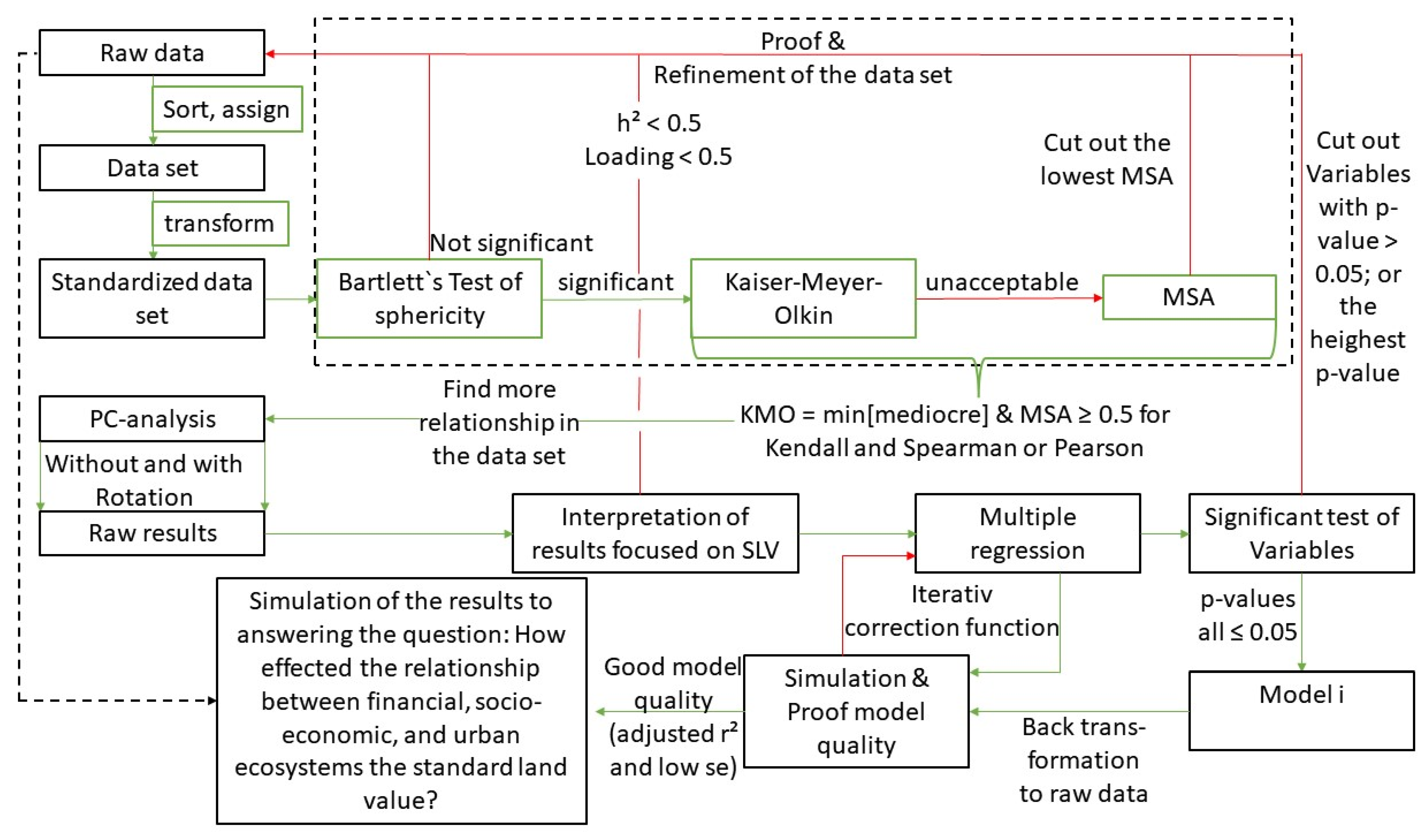
2. Materials and Methods

For the present analysis, a data set was created to identify the relationships between monetary, biotic and socio-economic aspects of urban land use. This analysis was focused on the state capital Magdeburg of the federal state of Saxony-Anhalt. The selected areas are in the districts of Altstadt (first documented mention in year 805), Stadtfeld Ost (first development in 1920s) and Stadtfeld West (first development in 1920s).
The SLRV level was determined on the basis of comparable areas. Accordingly, for reasons of consistency in the data set, a selective consideration of purely residential areas was undertaken. This was intended to exclude the effects of increased economic use. The observed area of Altstadt contains two spaces defined as residential area (RA), the rest was a mixed area (industrial and commercial side by side with residential area). Table 1 shows the total areas of each residential area with corresponding districts and their green spaces.
Twenty indicators were used, which might be related to land use. The 20 indicators whose correlations were examined in the following are: standard land reference value (SLRV), offered cold rents (OCR), interest on savings deposits (ISD), economic income (INC), inflation rate (IR), population density (INH), population density with migration background (IMIG), relative leaf area for trees on public green spaces and beside roads (LAI), number of tree individuals (Ntree), Evenness (Es), proportion of green spaces including private gardens per inhabitants (GS), biodiversity index according to Gloor [32] (BDI), weighted average distance to the nearest allotment garden (AlG), as well as to the nearest large green area (min_GI), the nearest water surface (Water), to schools (school), to medical treatment (min_med), to public transport (tra), the nearest retailer (ret), and to the nearest restaurant (rest_pkt).
The respective prices of the SLRVs are taken for the corresponding points in time from [33] and entered manually in a spreadsheet document. The stored time series amounted to between 2006 and 2020. The extents of the areas under consideration were manually accounted for in Quantum GIS (QGIS). A corresponding layer has been created for this purpose. There are a total of twelve residential areas, which were specifically considered as described below. An illustration can be seen in Figure 1.
The OCR was provided as an average per block [34]. For the year 2020, the 1st quarter of 2021 was scheduled. The different OCRs were calculated for the respective SLRV ranges using a weighted average. For this purpose, the mean OCR per block was summed over the number of blocks in the SLVR and then divided by the number of blocks in the SLVR. The OCR could not be generated completely until 2006. Only time series from 2011 to 2022 were available [35]. Furthermore, a linear growth of OCR was assumed. For this purpose, a model equation in the form y = mx + n was used for the respective rental apartment sizes (30 m2, 60 m2 and 100 m2). Here, y is the searched OCR at time x (year; Y). The following Equations (1)–(5) are used for OCR:
OCR30,i = 0.1236 × Y − 243.0481 ± 0.20 EUR/m2,
OCR60,i = 0.1301 × Y − 256.8140 ± 0.09 EUR/m2,
OCR100,i = 0.1825 × Y − 361.7568 ± 0.29 EUR/m2,
meanOCRi = (OCR30,i + OCR60,i + OCR100,i)/3
OCRm,i = 0.1454 × Y − 287.2063 ± 0.17 EUR/m2.
OCRm is the estimation function for the mean values with equal distribution of the different apartment sizes, which is rarely the case. Accordingly, a correction factor was introduced for each of the different SLRVs, which considers the inhomogeneous distribution of housing supply. Equation (6) shows the determination of the correction factor.
fc,j = OCRj,2020/OCRm,2020
This assumes that the correction invoice does not undergo any significant change over time. This was based on the ratio of the forecast value OCRm, 2020 (in 2020) with the actual OCR in the respective SLRV j (j = RA1 to RA12) in 2020. The estimation of the mean OCR for the area to be considered is performed using Equation (7).
OCRm,j,i = fc,j × OCRm,i
The next chosen indicator was interest rates on savings deposits. The underlying consideration is the relocation of financial values to real estate due to better returns. The evaluation “Development of the average interest rate for savings deposits in Germany in the years from 1975 to 2022” [36] was used as the data basis.
Next, the assets are considered. These are taken as income values for society. No regionalization was carried out here, as investments in real estate are usually not made by residents. This is especially true for properties that are used for rent. The underlying database consists of the one hand of the number of employees within Germany (E) [37] and on the other hand the mean income of the employees (INCa) [38], these two values are given to the Income Indicator (INC) by Equation (8):
INCj = Ej × INCaj
The inflation rate was taken into account based on Deutsche Bank’s records [39].
The density of people was provided for the SLRV areas examined by the City of Magdeburg, City Planning Office. An address-related distribution of persons is not possible for data protection reasons. In order to be able to incorporate the distribution of people for the next steps, the inhabitants were assigned to the buildings. The buildings were made available online by the State Office for Surveying and Geoinformation Saxony-Anhalt [40]. The buildings were first tailored to the SLRV areas studied and then the approximate people were distributed. For the three districts that are home to the SLRV areas studied, corresponding migration movements are known. Ziegler’s [41] explanations provide the database for the respective districts with the corresponding years as an assignment variable. For the calculation of the initial variable, the current persons were divided by the persons in the corresponding district. The relative person now obtained (persons of the SLRV area per person of the district) was multiplied by the annual person sizes of the districts. Persons with a migration background are also included in the statistics and taken into account as a separate influencing factor. The persons per SLRV area were divided by the corresponding area (ASLVR, see Table 1). Furthermore, the density of persons and persons with migration background (P) are obtained.
INHi or IMIGi = Pi,j,k/ASLVR,j
The next indicator was the leaf area index (LAI) at the respective time i in the respective SLRV area j. For this purpose, the tree cadastre of the state capital Magdeburg was used [42]. Following Kardan [10] and Kalusche [43], we used a maximum unilateral leaf area of 500 m2 per tree individual. In general, leaf area differs among tree species. We reduced these individual allometric growth conditions to a general approach. The tree individuals were determined for each area studied. After that, the crown diameter (cd) and tree height (h) were chosen to approach the leaf area per tree individual (indices t). According to Fauk and Schneider [44], the individual growth of trees has many influencing factors. These complex interactions between biotic and abiotic environment cannot be considered in this study. However, we used the knowledge about the general growth conditions for urban trees in the city of Magdeburg to introduce a simple model for crown expansion and height growth. We assumed an annual crown diameter growth of 0.5 cm and a height increase of about 1 cm. These values are to be considered conventional. Equation (10) shows the approach used.
LAi,j,t = [500 × (1 − exp(−((cd − (0.005 × ∆Y)) × ((h − (0.01 × ∆Y))/3)/100))) + 1]
To finally establish a relationship between the individual components or indicators, the individual leaf area had to be summed up first for the corresponding year i and the residential area j (see Equation (11)).
LAi,j = ∑LAi,j,t
For the summed leaf area to ultimately be converted to functional and comparable unit, an area reference to the respective residential areas had to be established. This was performed using Equation (12).
LAIi,j = LAi,j/ASLVR,i,j
Next, the biodiversity of the trees was determined. For this purpose, the Shannon Index was used first (see Equation (13)). The individuals per tree species was divided by the total number of tree individuals; the proportion of the respective tree species obtained in this way was multiplied by pj,i. Ultimately, the Shannon Index was calculated as a measure of plant diversity as follows:
HSj,i = −∑ pj,i × ln(pj,i)
This index only gives information about the number of species and their distribution, i.e., the diversity. However, it was important for us to consider the balance of species in the respective residential area. For this purpose, we used the species equitability (Es). For the calculation, the number of species (S) of all studied residential areas was used. The species equitability is also called evenness and was determined with Equation (14).
Esj,i = HSj,i/ln(S)
The green spaces (GS) for the respective residential areas were measured using NDVI (normalized difference vegetation index) [45]. The NDVI was determined using orthophotos (RGBI). These were provided by the State Office for Surveying and Geoinformation [40]. The NDVI gives values between −1 and 1. In order to determine GS, a reclassification had to be made. Based on comparative analyses, the green areas for the respective time point were matched with the NDVI values and a threshold of 0.15 was defined. These values can differentiate depending on the time of recording and must be determined manually or with machine learning algorithm. All values of the NDVI map that were greater than 0.15 were marked with 1 and the rest with 0. Subsequently, all pixels (0.2 × 0.2 m) within the respective residential areas were summed and multiplied by 0.04 m2. For this purpose, the raster calculator and the zone statistics of the QGIS software were used and the data was transferred to the residential areas. Finally, the calculation of the GS proportion was carried out per inhabitants for the respective residential area and is shown in Equation (15).
GSj = (AGI,j/∑Pj,k)
The next indicator is the Biodiversity Index (BDI) according to Gloor [32]. The BDI contains the faunistic biodiversity based on indicators species (birds, butterflies, bees, cicadas) for typical urban trees such as oak (Quercus robur, L.) or tree of heaven (Ailanthus altissima, (Mill.) Swingle). In general, neophytes show a smaller contribution to the biodiversity of native fauna than their native equivalent. The previously selected tree species and their number were multiplied by the corresponding BDI according to Gloor for the respective residential area and divided by the number of tree individuals in the respective residential area (weighted mean).
The indicators and their selection are briefly explained. We have generally opted for distance as the value for accessibility. At this point, we simplified accordingly and only considered the distance as the crow flies instead of the actual route.
The first indicator to be explained is the allotment gardens (AlG). Schneider and Fauk (2022) [46] pointed out that allotment gardens play an important role in the future production of regional food, while at the same time they form a potential to link natural areas as well as to preserve genetic diversity. This is underlined by our own observations in the allotment garden association Schnarsleben; the vegetation studies of different fallow areas indicate a settlement and establishment of protected (Aquilegia vulgaris, L.) and or rare (Dictamnus albus, L.) plant species. In view of the monocultural landscape character in the area concerned, a previous deliberate establishment of the plant species through horticultural activity is to be assumed. Accordingly, the cultural value of allotment gardens is to be estimated.
The nearest large green area (min_GI) where recreation and relaxation could be found, and, thus, an important contributor to cultural and regulating ecosystem services, were also determined as the crow flies. In this indicator we have considered cemeteries, grasslands, woodlands and nature reserves. We did not consider individual preferences of the population, but only the shortest distance.
The distance to the nearest water area (Water), which was also determined as the crow flies, should take into account both the function as a ventilation pathway in the terms of urban climatology and the importance of aesthetics. We have taken large as well as smaller standing and flowing waters as a basis.
The distance to schools (school) indicator was determined independently of the age structure of the population. A correspondingly in-depth database was not available. Furthermore, the distance was determined as the crow flies from the respective buildings and averaged over the residential areas. The shortest distance to medical treatment (min_med), the distance to public transport (tra), the distance to the nearest retailer (ret) and the distance to the nearest restaurant (rest_pkt) also determined as a crow flies. These indicators are intended to represent care and connectivity.
All distance indicators were measured using the distance tool in QGIS version 3.18.3. The linear distance was used, which takes into account the distance from the respective building in the corresponding residential area to the center of the indicator under consideration. These distances were weighted according to the buildings and estimated persons. The geodata were loaded into QGIS by the open street map extension and then used for the evaluation.
First, the connection, as shown in Figure 2, was assumed.
For further analysis, the software RStudio was used. First, the data set was standardized and centered. The data matrix has the dimension (156 × 20) and is denoted as Z.
First, the data set was tested for the hypothesis that:
H0 
: The variables in the survey population are uncorrelated.
H1: 
The variables in the survey population are correlated.
For this purpose, Bartlett’s test of sphericity [47] was used. The test value is strongly influenced by the sample size [48]. Chi-square (X2) was used as a test variable for assessment. The significance level was determined from the sample size (N), the number of variables (v) and the determinants of the correlation matrix (det(R)) using the degree of freedom (df = (v × (v − 1))/2).
X2 = −ln(det(R)) × (N − 1 − (2 × v + 5)/6)
At this point, the different correlation methods should be pointed out. These will play a significant role in the following assessments. Basically, a distinction is made between rank correlation and correlation coefficients. The rank correlation coefficient is determined according to the Kendall Equation (17) and the Spearman Equation (18). As the name “rank” suggests, only the place in an ordered list is considered. For Kendall’s rank regression, the concordant (C) and discordant (D) data pairs are used. For the subsequent normalization, the ties between variable Y (Ty) and variable X (Tx) are taken into account.
τ = (C − D)/[(C + D + Tx) × (C + D + Ty)]0.5
For the Spearman rank regression, the respective ranks (R) and their mean values (Rm) are considered.
rs = ∑i (R(xi) − Rm,x) × (R(yi) − Rm,y)/[(∑i (R(xi) − Rm,x)2)0.5 × (∑i (R(yi) − Rm,y)2)0.5]
The Pearson correlation coefficient is determined using the data values (X, Y).
rp = ∑i (Xi − Xm) × (Yi − Ym)/[(∑i (Xi − Xm)2)0.5 × (∑i (Yi − Ym)2)0.5]
Subsequently, the suitability of the data set was tested using the Kaiser–Meyer–Olkin (KMO) and the MSA criterion (package: EFAtools [49] and factoextra [50]). The Kendall, Pearson and Spearman regression methods were used. The KMO criterion considers all variables of the data set [48] and was calculated with the equation.
KMO = ∑ii’ (rxixi’)2/[∑ii’ (rxixi’)2 + ∑ii’ partial_(rxixi’)2]
The measure of sampling adequacy (MSA) tested the single variable for fitness [48]. For this purpose, we have used the equation.
MSA = ∑i’ (rxixi’)2/[∑i’ (rxixi’)2 + ∑i’ partial_(rxixi’)2]
A partial correlation (partial_(rxixi’)) is defined as a correlation between two variables with no further influence from the other variables [48].
The next step was a principal component analysis. This was used for the initial interpretation of the data. The unknown matrices S, which contains the factor values and L, which contains the factor charges, reproduce the standardized initial matrix Z. This is generally expressed by Equation (22):
Z = S × L
By transforming and substituting the correlation matrix (R = 1/(N − 1) × Z’ × Z), assuming the uncorrelated nature of the data for principal component analysis, it follows (Backhaus et al.) [48]:
R = L × L’
The PCA was performed without and with rotation of axes.
Figure 3 shows that the raw results from the PCA have been further processed. The scores of the indicators on the newly created axes can be interpreted differently depending on the application. This individuality offers a correspondingly large space for interpretation of the results and corresponding discussions. For this purpose, reference will be made to the relationship between financial, socio-economic and urban ecosystems (which can provide ecosystem services) on standard land values. For our investigation, it was not important whether an indicator loads on one of the new components, but rather the multiple loading of an indicator. The goal was to identify as large an explanation of the variance as possible, especially for the SLRV. In accordance with good practice, the results of the new dimensions (scores) were considered with the communality ( h j 2 = q = 1 Q a j q 2 ) per variable. We did not use the normal criteria to remove variables from the data set for further principial component analysis. The first step was to find the dimension where the score for the SLRV was greater than or equal to 0.5. Subsequently, the individual variables were considered in the respective dimension. If a score was smaller than 0.5, we first looked for other dimensions in which SLRV and the respective variable loaded above 0.5. If no further dimensions could be found, it was checked whether the variables were smaller than 0.3, and analogous to the previous procedure, a further step was introduced. Now the explanatory variance of the respective dimensions was tested, as well as the significance of the variables based on the communality after exclusion of the unused dimensions.
The final step was to interpret the PCA results and build a multiple regression model to predict SLRV based on the identified indicators or variables (I). For this purpose, we established a linear relationship to the indicators or variables. The general form of the equation can be seen in the equation. For the first model, the coefficients of each variable were determined using the standardized data matrix. Since the manipulation of data sets in terms of standardization or logarithmization may have a bias in the back transformation, two fitting models were implemented.
SLV = c1Ii + c2Ii+1 + … + cnIi+n
The simple linear fitting model 1 Equation (25).
SLV1 = b + m × SLV
The simple quadratic fitting model 2 Equation (26).
SLV2 = b + m × SLV + n × SLV2

3. Results

3.1. Results of Data Matrix Test and Data Refinement Procedure

The Bartlett’s test for sphericity was significant at an alpha level of 0.05 for all iteration steps (Pearson: start (X2(190) = 6667.64, p < 0.001), iteration 8 (X2(66) = 2099.27, p < 0.001)). These data are probably suitable for factor analysis. A singular matrix was reported for the rank correlation (Kendall, Spearman). This indicates correlated values in the initial matrix. Accordingly, the further procedure (KMO and MSA) was based on Pearson’s method, while Kendall’s and Spearman’s methods were not considered further. Since Bartlett’s test only shows the principal suitability of the data set, the Kaiser–Meyer–Olkin criterion with the respective MSAs served to fit the data set. Each exclusion of a variable can have a large effect on KMO and MSA, only single variables (indicators) were removed. The initial data set had a KMO value of 0.374 and was classified as unacceptable. Based on the MSA criterion, min_gi (0.160) was removed. For iteration 1, there was an increase in KMO to 0.407 (unacceptable). The indicator BDI (0.145) was excluded. Iterations 2 (KMO = 0.395 and MSA excl. = ret (0.163)), 3 (KMO = 0.368 and MSA excl. = tra (0.203)) and 4 (KMO = 0.466 and MSA excl. = LAI (0.284)) were also unacceptable. The first iteration to show a miserable result for the KMO value (0.562) was number 5. Evenness was excluded based on the MSA of 0.301. Analogous to iteration 5, iteration 6 also showed a miserable KMO score (0.595). Based on the lowest MSA, Water (0.382) was extracted. Iteration 7 and 8 were both mediocre (Iter. 7 = 0.641 and Iter. 8 = 0.661). After iteration 7, IMIG (0.483) was removed. Iteration 8 indicated SLRV (0.495) as an indicator to be extracted, so the final data set was reached at this point. The full results are given in Table 2.

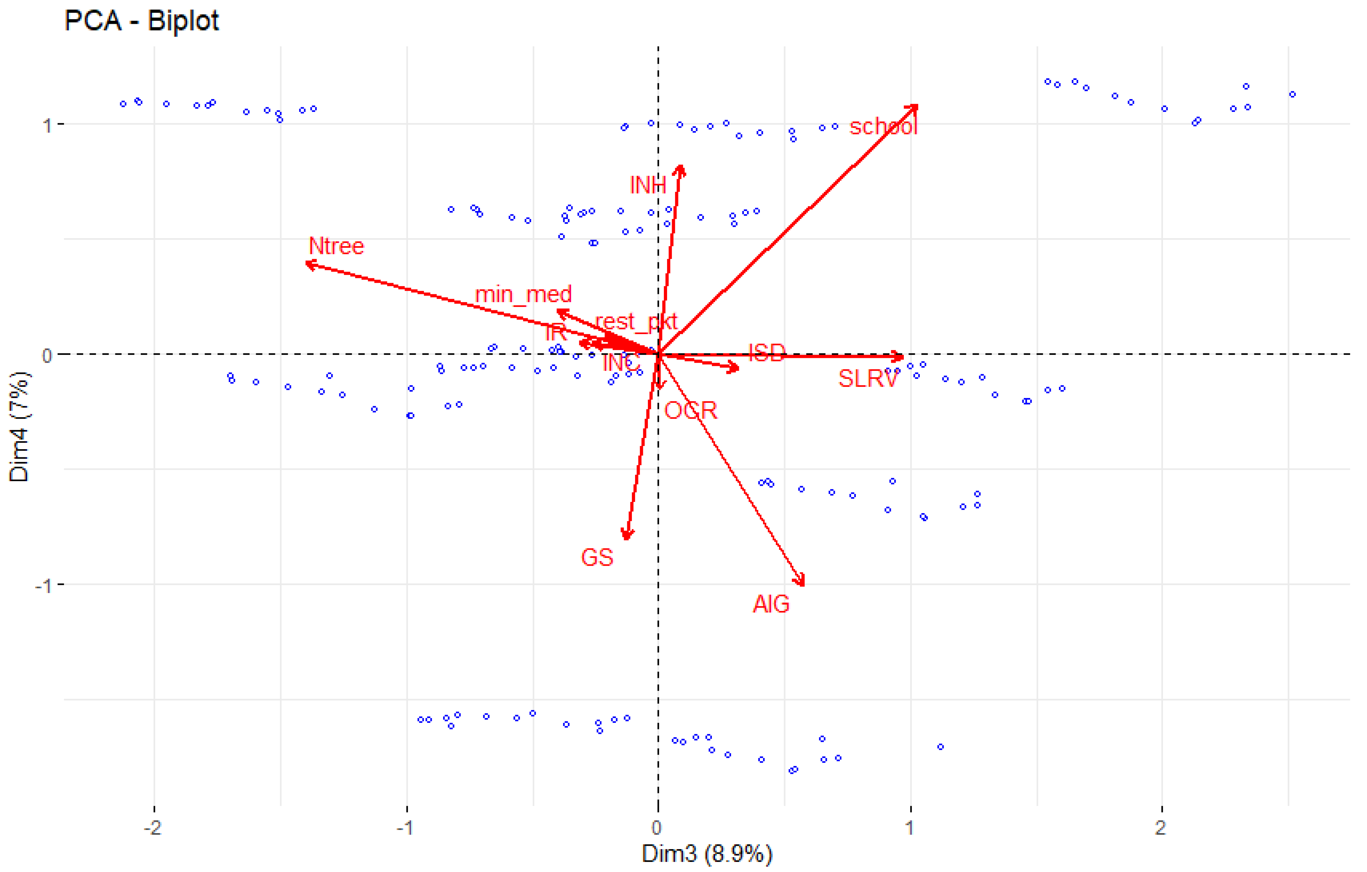
3.2. Evaluation of the PC Analysis

Due to the good test results in the Bartlett test and the KMO test, the principal component analysis was performed. The correlation matrix provides 12 dimensions (principal components), 8 of which explain ≈ 98% of the variance in the data set. Before the important dimensions are considered more decidedly, they should first be derived optically or on the basis of the explained variance. Figure 4 shows a first clear bend on the third dimension. However, a roughly equal explained variance could be found for dimension four (explained variance > 5%). The summed explained variance in the data set was 79.4% for the third dimension (principial components) and86.3% for dimension four.
The first two dimensions represent 70.46% of the variance in the data set and can be seen in the Figure 5. Dimension one correlates most strongly with GS (r = 0.7615) and INH (r = −0.7719). Other positively influenced indicators by dimension 1 are: rest_pkt (r = 0.7248), min_med (r = 0.7405) and school (r = 0.5361). On the other hand, there are the negatively influenced indicators, such as AlG (r = −0.6744) and SLRV (r = −0.6730). Overall, 37.20% of the variance was described in this dimension. Dimension two correlates most strongly with ISD (r = 0.8346). Negatively correlated are INC (r = −0.8631) and OCR (r = −0.8388) and IR (r = −0.8500). This dimension describes 33.26% of the variance in the data set.
Dimensions three and four describe 15.88% of the variance in the data set and are shown in the Figure 6. Dimension 3 correlates most strongly with the indicator Ntree (r = −0.6464). This dimension describes about 8.91% of the variance. The fourth dimension correlates with school (r = 0.5132) and describes 6.97% of the variance.
Now the PCA analysis was used to check whether further indicators can be reduced. For this purpose, the dimensions were first reduced without lowering the explanatory variance of the indicator below 0.3. The PCA result was reduced to three dimensions. The explanatory variance of the data set was thus reduced to 79.37%. Moving on, the focus was now on SLRV, for which h2 was used after reducing the dimensions. The initial h2 for SLRV was 1 (normal for PCA analysis). After reducing the dimensions, the commonality was 0.8220. h2 for all other indicators was greater than 0.5 and the absolute minimal score in one of the three dimensions was greater than 0.5. All in all, no further indicator exclusion was performed by the PCA analysis. In the case of a PCA, the indicators shown in green would each have to be assigned to the dimensions individually. Dimension 1 showed that the standard land value could apparently only be described by social factors and the green infrastructure. However, the communality for SLRV was then only 0.4530 (45.30% explained variance of the variable SLRV). In the second dimension, only loadings of the financial indicators greater than 0.5 were evident, and an absolute loading greater than 0.3 was still recorded for SLRV. We do not exclude SLRV and with the dimension 2, we obtain a communality of 0.6124. This 61.24% explained variance was not enough for us either. Furthermore, the number of trees would have no influence at this point and this variable would be described incompletely (h2 = 0.3848). With the dimension 3, on the one hand, a significant part of the communality for SLRV (h2 = 0.8220) could be described; on the other hand, the contribution of the city trees was identified by an absolute loading >0.5. The SLRV charge was close to 0.5, which was why a connection had to be assumed. The fourth dimension can be largely ruled out, (a) no significant loading of the variable SLRV, (b) double loading of School, which is why it was already described in the previous dimension. The PCA analysis showed that initially all 12 variables should be used for further multiple regression. The PCA scores are shown in the Table 3 for three Dimensions. The full PCA result can be seen in the Table 4.

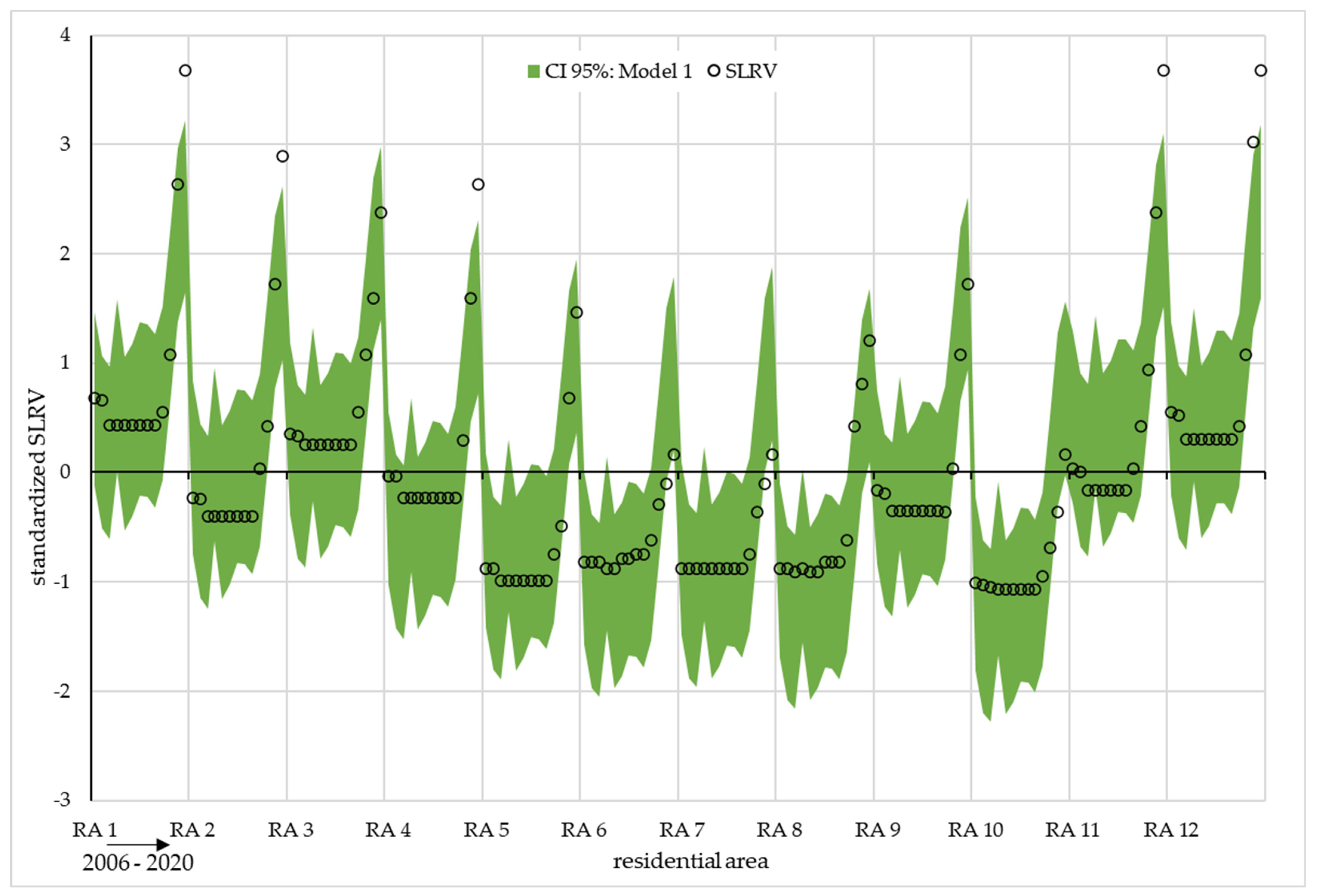
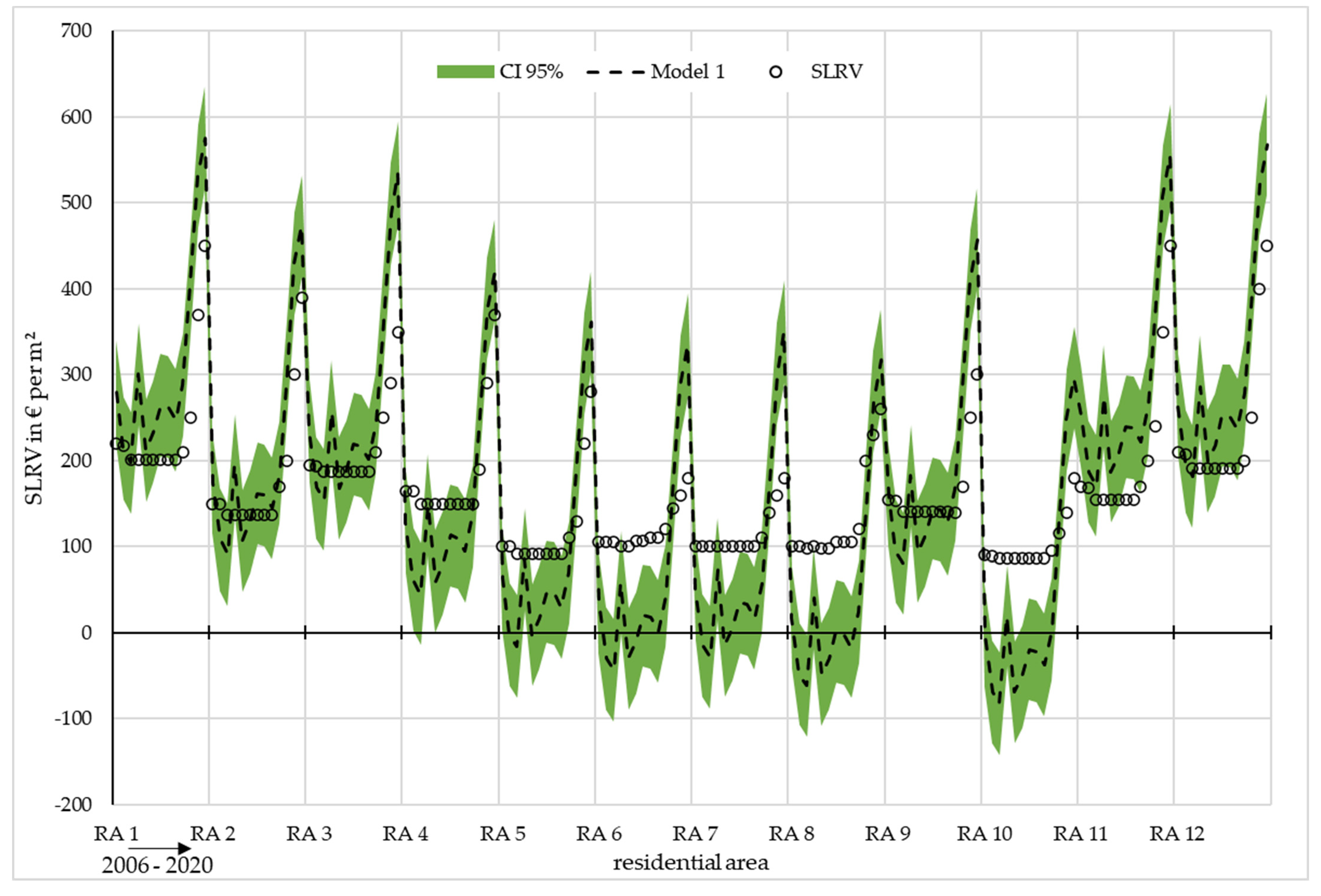
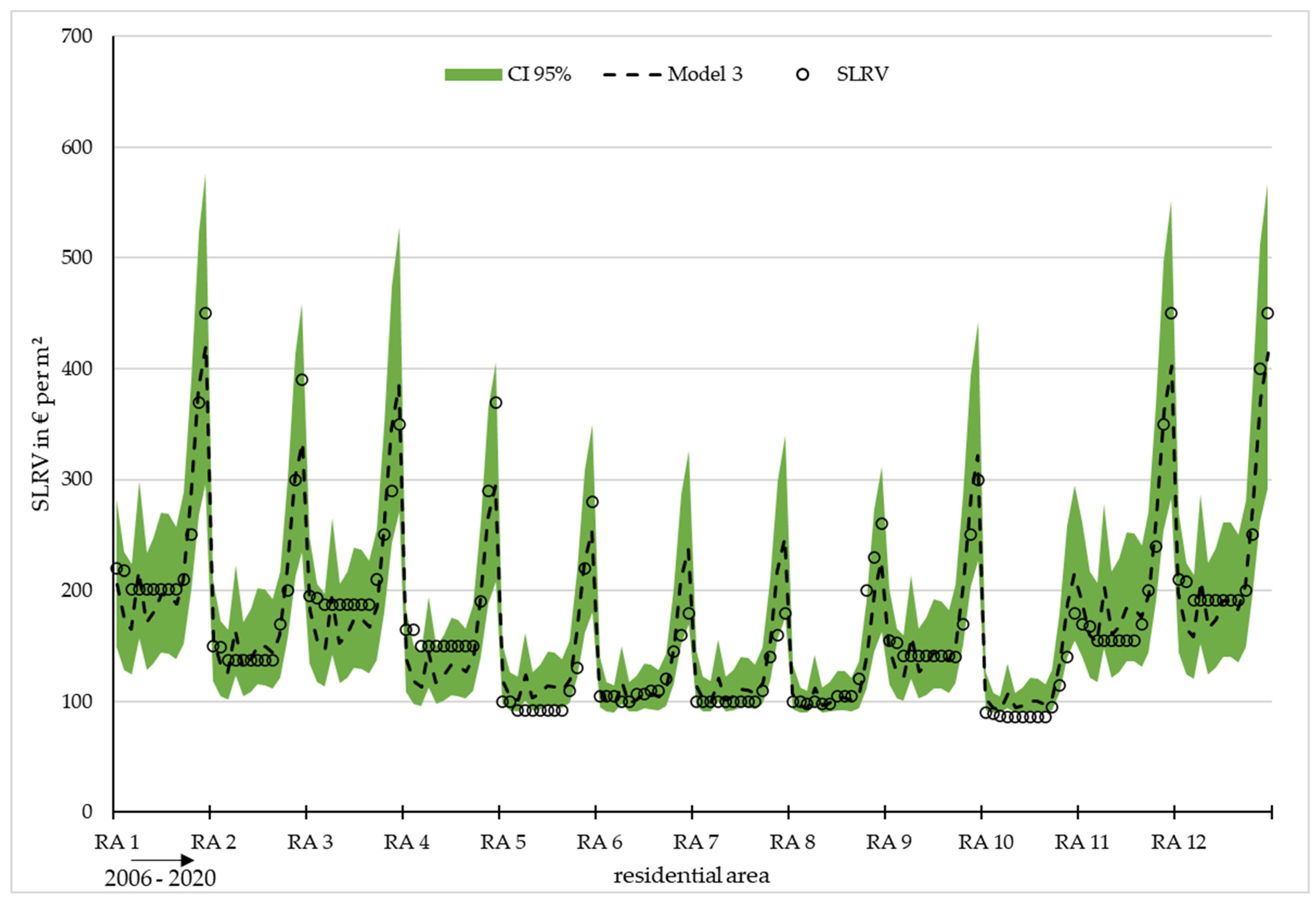
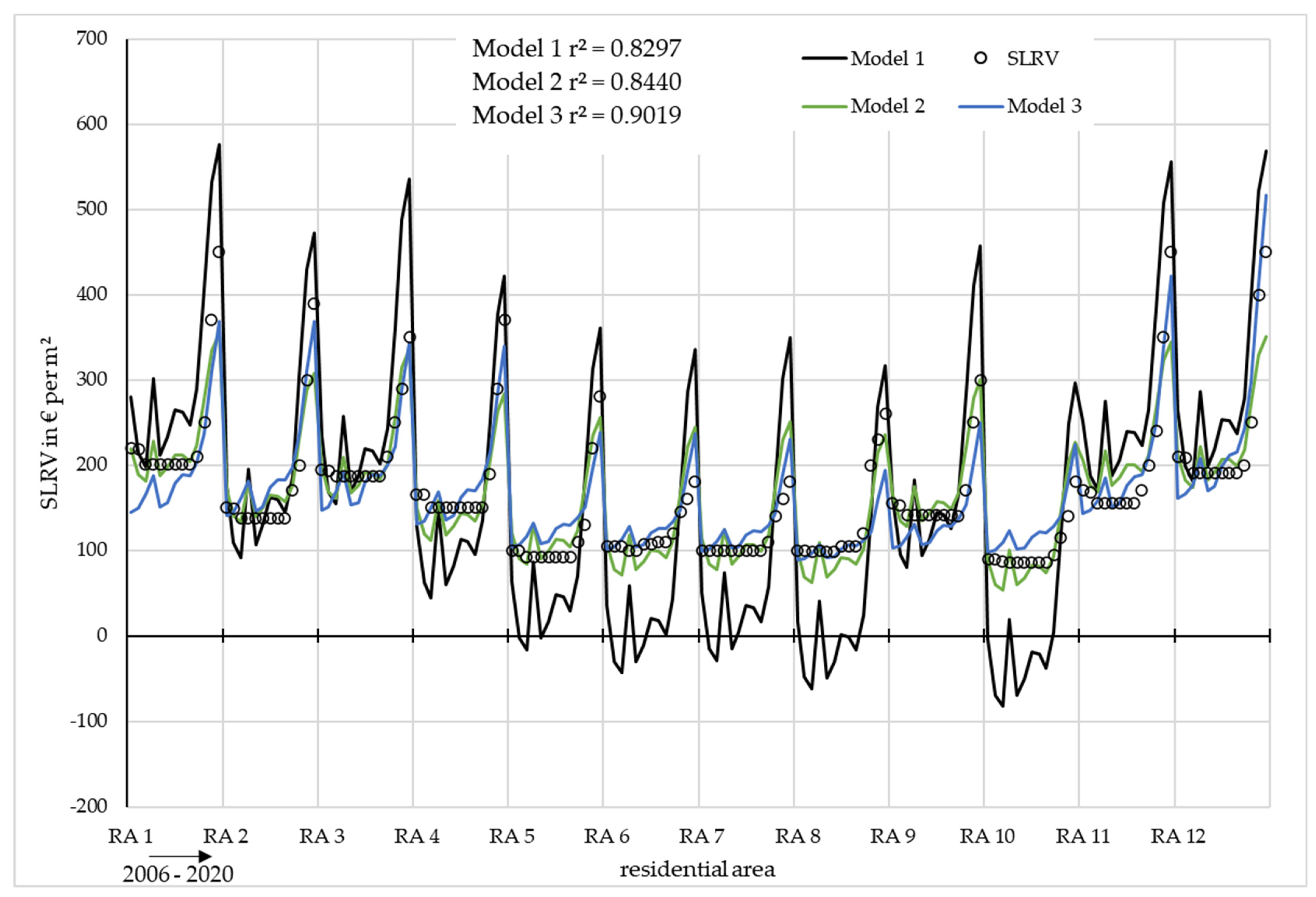
3.3. Results of the Multiple Regression

The multiple regression for the 11 indicators (after rearranging the indicators for multiple regression) shows no significance for the variable OCR (p = 0.7449) in the first iteration step. We have removed the variable before the next iteration. The second iteration showed no significance for the indicator GS (p = 0.2640). The third iteration showed all variables to be significant. For further information see the Table 5.
The basic model for determining the individual effect sizes of the variables examined was based on a standardized data set (mean = 0 and standard deviation = 1). A corresponding comparability of the baseline situation was given. Before the effects are quantified in the following chapter, a basic evaluation of the charges on the variables was carried out at this point. The largest charges or effects are given by the variables INC (c = 2.5286, p < 0.05), IR (c = −1.3472, p < 0.05) and ISD (c = 0.6203, p < 0.05). It became clear that the financial sector, with the variables’ Germany-wide labor market situation with corresponding income, as well as the inflation rate had the greatest influence on the standard land values. A variable from the financial sector (ISD) was also identified as having less influence but was the third largest. Distance to the nearest medical facility (min_med c = −0.3928, p < 0.05) and to the nearest allotment garden (AlG c = 0.3255, p < 0.05) were the next largest influencing variables. The last variable to take on a more profound significance in our research question was the number of trees with c = −0.1871 (p < 0.05). For a complete overview of the variables and the corresponding statistics, please refer to Table 5.
Since standardized values were used for the initial model (see Figure 7), the mean value of the SLRV could be used to back-calculate to the functional unit. The back calculation had this form SLRV = SLRV mean + SLRV result × SLRV mean. Due to standardization, SLV result = 0 means that SLRV must take the value of SLRV mean. Since a drift of the forecast for a residential area was evident due to the standardization (see Figure 8). The back-calculated model 1 has a RMSE of EUR 88.65 per m2. Now, another improvement of the model has been made. For this purpose, linear and quadratic functions were used. The linear function could not improve the multiple correlation coefficient (r = 0.9192), but the model quality improved from adj. r2 = 0.8297 to adj. r2 = 8440. The RMSE was EUR 30.12 per m2. The quadratic equation for model fitting yielded an improvement in the multiple correlation coefficient (r = 0.9504) and that of the model goodness (r2 = 0.9019). The RMSE was EUR 23.80 per m2. The coefficients, as well as the parameter statistics, can be found in the Table 6 and Table 7. The graphical illustration can be seen in the Figure 9 and Figure 10. The comparison of the individual models was realized in the Figure 11.

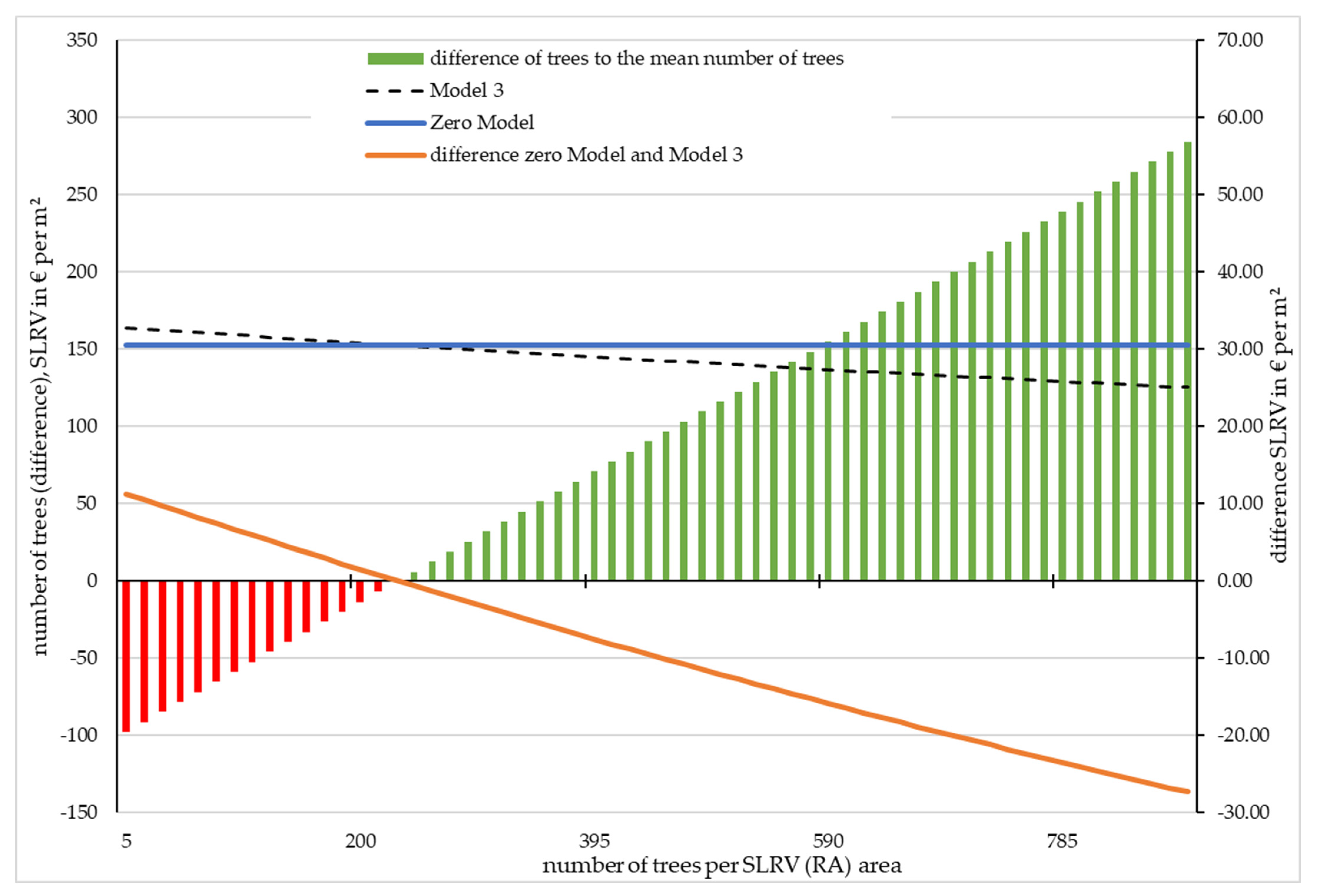
3.4. Relationship between the Standard Land Values and Components of the Green Infrastructure

After the extraction of indicators and the adjustment of the model quality, the focus will now be on the effects on the SLRV that are associated with a change in variables. From the regression, it was evident that INC had the greatest influence, so to describe the interaction between SLRV, Ntree and AlG, we must out clouded effects from other variables. For this we had made the two scenarios “tree planting” and “land transformation allotment garden”. It should be mentioned again that a standardized value of 0 is equivalent to the mean value of a variable. Accordingly, the interrelationships shown in the table are the initial situation for the scenarios. The baseline model is expressed in Table 8.
The next look is at the number of trees in public green spaces. Our database ranges from a minimum of 5 to a maximum of 828, with an average of 231 trees per residential area. A residential area with only five trees therefore had an estimated increase in value compared to the mean of EUR 11.22 (CI 95%: −7.94–27.82) EUR per m2. Meanwhile, an area with 830 trees was worth less by an estimated −25.19 (CI 95%: −45.16–1.75) EUR per m2. Simplified, it can be stated that the SLRV per percentage change from the average of trees individuals decreases by an average of 0.11 (CI 95%: −0.54–0.36) EUR per m2. Furthermore, a change of −52.5% in the number of trees caused a rising of 3.9 (CI 95%: −9.1–15.9) % in the SLRV. Likewise, an increase in the number of trees about 51.2% causes a decrease in SLRV of −3.6 (CI 95%: −17.1–10.7) %. Thus, the past 14 years indicate that in the evaluation of standard land values, urban trees as an important service provider for human health are considered in contrary contradiction or underrepresented. The result of the scenario “tree planting” was presented with the main parameters in the Figure 12 and with the 95% confidence interval in the Figure 13.
The results for allotments were like that for trees. In general, it could be deduced from the results that the standard land values increase with a change in percentage from the mean distance to allotment garden sites about 0.49 (CI 95%: −0.36–1.42) EUR per (m2 × %). The distance to the allotments ranged from 196 to 916 m in our data set, with an average of 421 m distance (crow flies). Thus, 195 m to an allotment garden site causes a reduction in the standard land value by 21.62 (CI 95%: −31.72–−14.30) EUR per m2. While an increase in the path distance to 990 m means that about 74.74 (CI 95%: 16.75–148.16) EUR per m2 more can be achieved. Furthermore, a change of −53.7% in the distance to the allotment sites caused a reduction of 14.2 (CI 95%: −20.8–−9.4) % in the SLRV. Likewise, an increase in the distance to allotment gardens of 53.2% causes an increase in SLRV of 17.0 (CI 95%: −4.6–41.6) %. The result of the scenario “land transformation allotment garden” was presented with the main parameters in the Figure 14 and with the 95% confidence interval in the Figure 15.
In summary, when comparing the effects, a change in the number of trees for 2006 is less pronounced than a change in 2020 (see Figure 16). While the estimated SLRV increased by about 187% between 2006 and 2020, the effect increased by 1424.5% for 800 trees and for 300 m distance to allotments, the effects increased by 1334.8%.
It can be positively stated that there was no evidence of “green gentrification” in the formation of SLRV. On the negative side, it appears that the cultural values and regulatory services of green infrastructure are not being considered. Furthermore, there is a risk that important urban ecosystems or their components will fall victim to profiteering. For example, allotment gardens offer great potential to produce regional food, while at the same time providing an educational contribution for young and old, as well as being important refuges for wildlife. With increasing distance to the allotment garden sites, on the one hand, the obstacle to visit them regularly increases. Also, the trees not considered analogous to the ecosystem services can be stated. Thus, a reduction in street trees can lead to a considerable thermal load in the summer months. The reduced leaf area yields a reduced filtering function in the context of particulate air pollutants. These important aspects are not interpreted or misinterpreted when determining the SLRV. Finally, the present study indicates that (a) a uniform evaluation matrix for the SLRV should be created, and (b) the present subjective land assessments by the relevant experts should be complemented through targeting further training in the ecologically oriented planning context.

4. Discussion

The first important point to be taken up in the discussion is the underlying database. On the one hand, only a relatively short period of land use change was available in the area under consideration. An expansion of the study area or number of residential areas could contribute to improving the validity of the results and their corresponding interpretation. Furthermore, it would be important at this point to include other regionalized social factors, such as the level of education or regional income (cf. Kardan). Instead of or as a supplement to the BDI, estimates from vegetation maps could be used. Referring to Methorst et al. (2021) [51], the actual diversity and abundance of birds should also be used.
There were hardly any data available for new buildings, the closure of vacant lots or the creation and management of green spaces. Also, there was no known change in the number and distance of the medical facility, public transport stop, schools and retail outlets for the respective objects considered. The offered cold rents are based on a linear function for objects <2011; corresponding errors must be assumed. The BDI according to Gloor et al. 2018 [32] was strongly dependent on the tree species and their number, which was why there might be a relation. However, a high BDI indicates native tree species such as Quercus robur, T. cordata or the genus Malus. The test procedures were met, except for the KMO criterion for Kendall and Pearson.
The principal component analysis revealed loadings in two dimensions for all indicators, so that principal correlations were highlighted. Therefore, some significance can be assumed. Overall, however, it should be noted that the commonality for SLV is only about 0.8. Conversely, about 20% of the variance for SLRV could not be explained. This is why multiple regression was used to identify the effects of the indicators on SLRV.
The initial eleven indicators, which were supposed to describe SLRV after conversion, could be further reduced due to significance. The multiple regression showed that large effects of market economy (INC, IR and ISD) are significant for the pricing of standard land values. For green infrastructure, allotments showed the larger effect. This indicator can be interpreted as increasing densification of the settlement area. The largest distances were evident from the highly dense core areas (especially WG 11) or areas with old development structures. It can be stated based on the examined areas and the available database that for every meter distance to an allotment site, the SLRV increases by 0.49 (CI 95%: −0.36–1.42) EUR per (m2 × %). This may well be methodical, as allotment garden sites are readily used by ecological lending in planning offices as well as local government for land development. Despite all the discussion about species extinction, loss of genetic diversity and formation of resilience for the urban ecosystem, it is not the monocultural agricultural land with almost no benefit, except for a food production, but important urban ecosystems that are required of great importance for sustainable design that are decimated. Now, if the adjacent area is “favorable”, after the land use change from allotments to settlement area, the SLRV of the adjacent settlement area is used.
The tree individuals showed analogous results such as allotment gardens; here too it can be generalized that the less “green”, the higher the SLRV. Highly developed urban areas usually do not offer space for many tree plantings, but seem to have value in terms of grey infrastructure. In the densely populated areas, the existing tree pits are not revitalized even after the trees have died. Furthermore, the SLRV does not provide an incentive to bring greener into the city.
If it is now assumed that public landowners want to achieve the highest possible financial benefit and are guided by the SLRV, no tree planting or other green infrastructure elements are required. However, it is imperative to note that the SLRV does not represent the asking prices; in structurally weak regions the properties are sometimes classified with, e.g., 20% of the SLRV. It is, therefore, imperative to carry out further investigations that represent a more detailed model. The focus here is on, for example, the value of ecosystem services in districts and the corresponding asking rents or the land or real estate sales prices.

5. Conclusions

Against the background of the social transformation towards a climate-neutral, ecologically oriented society, it is likely that there will be a change in mentality with regard to space marketing. Large real estate marketers are now also dealing with the ecological potential of their areas and their ecosystem services as a market argument and are having their areas ecologically upgraded. This development represents an opportunity for tasks of the century. In addition to the SLRV investigation, the determination of CO2 binding potential, soil resources (e.g., for water retention in the area), fine dust binding potential and biomass resources represent criteria with which a quantitative upgrading of the areas can be balanced, and should be subject to future investigations.
In the future, the ecological quality of the outdoor facilities, for example, can also be an award criterion when determining the “most economical offer” for construction measures. In order to be able to allocate the costs and benefits of green spaces in the future, for example, in the award procedure, the entire life cycle costs of green spaces must be taken into account during planning, maintenance and demolition.
Sufficient areas are needed for green spaces, even in conurbations with high settlement pressure. Vertical green cannot fully replace the loss of green space. It is, therefore, important to also use the potential of unused areas for urban green spaces. Successful municipal land recycling has a high symbolic power for the establishment of a circular land use economy, in which one use becomes a prerequisite for the subsequent one and where a site, as a whole, remains in use in the long term. To the extent that fallow land is successfully reused, further concepts for saving land gain in persuasiveness (Dosch et al. 2006 [52], Jakubowski et al. 2007 [53]).
New planning processes, procedures and instruments are needed as part of green space governance. These should inform citizens and owners early and comprehensively about the future use and design of properties and at the same time address the ideas and needs, worries and concerns of the resident population. In addition, citizens are asked to contribute their energy, time and creativity to the design of communally usable properties for the benefit of the general public. This is known internationally as the Land Governance Assessment Framework (LGAF), which aims to improve the transparency of usage decisions and contributes to private owners being involved in offsetting land value increases through green spaces (called direct and indirect value capture in Anglo-Saxon countries).

Author Contributions

Conceptualization, P.S. and T.F.; methodology, T.F.; software, T.F., validation, P.S.; formal analysis, T.F., investigation, T.F.; resources, P.S.; data curation, T.F., writing—original draft preparation, P.S.; writing—review and editing, T.F.; visualization, T.F.; supervision, P.S.; project administration, P.S.; funding acquisition, P.S. All authors have read and agreed to the published version of the manuscript.

Funding

This research received no external funding. It was performed within the activities of the working group Ecological Engineering at Magdeburg-Stendal University of Applied Sciences.

Data Availability Statement

Data are available from the authors upon reasonable request.

Conflicts of Interest

The authors declare no conflict of interest.

References

  1. LABO Bund/Länder-Arbeitsgemeinschaft Bodenschutz (Hrsg.) (2012): Reduzierung der Flächeninanspruchnahme. Statusbericht zu den LABO-Berichten vom 21.09.2011 sowie 30.03.2010. Bericht zur Vorlage an die Umweltministerkonferenz. Available online: https://www.labo-deutschland.de/documents/1_Anlage_LABO_Reduzierung_der_Flaecheninanspruchnahme_f11.PDF (accessed on 14 October 2015).
  2. Hoymann, J.; Goetzke, R. Flächenmanagement, pp. 154–196, ARL—Akademie für Raumforschung und Landesplanung (Hrsg.): Handwörterbuch der Stadt-und Raumentwicklung Hannover 2018, ISBN 978-3-88838-559-9 (PDF-Version). 2018. Available online: http://nbn-resolving.de/urn:nbn:de:0156-55993 (accessed on 10 July 2023).
  3. Ingenieurtechnischer Verband Altlasten, e.V. (ITVA), Berlin 1998, 25 S., Erarbeitet im ITVA-Fachausschuss C 5 Flächenrecycling“. Available online: https://www.itv-altlasten.de/publikationen/arbeitshilfen-und-richtlinien/flaechenrecycling.html (accessed on 28 June 2023).
  4. Bundesministerium für Umwelt, Naturschutz, Bau und Reaktorsicherheit (BMUB). Grün in der Stadt—Für eine Lebenswerte Zukunft; Grünbuch Stadtgrün: Berlin, Germany, 2015. [Google Scholar]
  5. Government of Germany; Thiel, F. Wertsteigerung Durch Grünflächen—Wer Profitiert? Informationen zur Raumentwicklung: Bonn, Germany, 2016; pp. 691–701. [Google Scholar]
  6. Schneider, P.; Fauk, T.; Mihai, F.-C. Reclaiming Urban Brownfields and Industrial Areas-Potentials for Agroecology. In Agroecological Approaches for Sustainable Soil Management; Prasad, M.N.V., Kumar, C., Eds.; Wiley: Hoboken, NJ, USA, 2023; pp. 409–436. ISBN 978-1-119-91198-2. [Google Scholar]
  7. Debus, M. Bodenrichtwertableitung in der Praxis. In Kreditwirtschaftliche Wertermittlungen. 8; Pohnert, F., Ed.; Auflage: Wiesbaden, Germany, 2015. [Google Scholar]
  8. Kleiber, W. Verkehrswertermittlung von Grundstücken, Kommentar und Handbuch. 7; Auflage: Köln, Germany, 2014. [Google Scholar]
  9. The American Society of Landscape Architects. Professional Practice—Green Infrastructure. 2019. Available online: https://www.asla.org/greeninfrastructure.aspx (accessed on 22 January 2019).
  10. Kardan, O.; Gozdyra, P.; Misic, B.; Moola, F.; Palmer, L.J.; Paus, T.; Berman, M.G. Neighborhood greenspace and health in a large urban center. Sci. Rep. 2015, 5, 11610. [Google Scholar] [CrossRef]
  11. Gann, G.; Lamb, D. Ecological Restoration: A Means of Conserving Biodiversity and Sustaining Livelihoods; Society for Ecological Restoration International: Tucson, AZ, USA, 2006. [Google Scholar]
  12. Fauk, T. Entwicklung eines biologisch-physikalisch basierten Ansatz zur Quantifizierung und Inwertsetzung ausgewählter Ökosystemleistungen von Dachbegrünungen als auch Dachbewässerungssystemen anhand des Stadtteils Stadtfeld Ost der Landeshauptstadt Magdeburg. Master‘s Thesis, Magdeburg-Stendal University of Applied Sciences, Magdeburg, Germany, 2021. [Google Scholar]
  13. Schwaiger, E.; Berthold, A.; Gaugitsch, H.; Götzl, M.; Milota, E. Wirtschaftliche Bedeutung von Ökosystemleistungen Monetäre Bewertung—Risiken und Potenziale. Umweltbundesamt. 2015. Available online: http://hdl.handle.net/11159/78 (accessed on 10 July 2023).
  14. Wittowsky, D.; Hoekveld, J.; Welsch, J.; Steier, M. Residential housing prices: Impact of housing characteristics, accessibility and neighbouring apartments—A case study of Dortmund, Germany. Urban Plan. Transp. Res. 2020, 8, 44–70. [Google Scholar] [CrossRef]
  15. Anderson, S.T.; West, S.E. Open space, residential property values, and spatial context. Reg. Sci. Urban Econ. 2006, 36, 773–789. [Google Scholar] [CrossRef]
  16. Boyle, A.; Barrilleaux, C.; Scheller, D. Does walkability influence housing prices? Soc. Sci. Q. 2014, 95, 852–867. [Google Scholar] [CrossRef]
  17. Cervero, R.; Duncan, M. Neighbourhood composition and residential land prices: Does exclusion raise or lower values? Urban Stud. 2004, 41, 299–315. [Google Scholar] [CrossRef]
  18. Li, W.; Joh, K.; Lee, C.; Kim, J.-H.; Park, H.; Woo, A. Assessing Benefits of Neighborhood Walkabiliy to Single-Family Property Values—A Spatial Hedonic Study in Austin, Texas. J. Plan. Educ. Res. 2015, 35, 471–488. [Google Scholar] [CrossRef]
  19. Lynch, A.K.; Rasmussen, D.W. Measuring the impact of crime on house prices. Appl. Econ. 2001, 33, 1981–1989. [Google Scholar] [CrossRef]
  20. Song, Y.; Knaap, G.-J. Measuring the effects of mixed land uses on housing values. Reg. Sci. Urban Econ. 2004, 34, 663–680. [Google Scholar] [CrossRef]
  21. Geurs, K.T.; van Wee, B. Accessibility evaluation of land-use and transport strategies: Review and research directions. J. Transp. Geogr. 2004, 12, 127–140. [Google Scholar] [CrossRef]
  22. Bourne, L. The Geography of Housing; Halsted Press: New York, NY, USA, 1981. [Google Scholar] [CrossRef]
  23. Hanhörster, H.; Lobato, R. Migrants Access to the Rental Housing in Germany: Housing Providers and Allocation Policies. Urban Plan. 2021, 6, 7–18. [Google Scholar] [CrossRef]
  24. Galvin, R. Do housing rental and sales markets incentivise energy-efficient retrofitting of western Germany’s post-war apartments? Challenges for property owners, tenants, and policymakers. Energy Effic. 2023, 16, 25. [Google Scholar] [CrossRef] [PubMed]
  25. Köhler, T. Bewertung ausgewählter Ökosystemleistungen im Grünzug der Goetheanlage Magdeburg, Master thesis an der Hochschule Magdeburg-Stendal, Studiengang Ingenieurökologie. Master’s Thesis, Magdeburg-Stendal University of Applied Sciences, Magdeburg, Germany, 2022. [Google Scholar]
  26. Ali, L.; Haase, A.; Heiland, S. Gentrification through Green Regeneration? Analyzing the Interaction between Inner-City Green Space Development and Neighborhood Change in the Context of Regrowth: The Case of Lene-Voigt-Park in Leipzig, Eastern Germany. Land 2020, 9, 24. [Google Scholar] [CrossRef]
  27. Bockarjova, M.; Botzen, W.J.W.; van Schie, M.H.; Koetse, M.J. Property price effects of green interventions in cities: A meta-analysis and implications for gentrification. Environ. Sci. Policy 2020, 112, 293–304. [Google Scholar] [CrossRef]
  28. Rigolon, A.; Németh, J. “We’re not in the business of housing”: Environmental gentrification and the nonprofitization of green infrastructure projects. Cities 2018, 81, 71–80. [Google Scholar] [CrossRef]
  29. Tsai, I.-C.; Lin, C.-C. Influence of migration policy risk on international market segmentation: Analysis of housing and rental markets in the euro area. Econ. Res. Ekon. Istraživanja 2023, 36, 2121740. [Google Scholar] [CrossRef]
  30. Mell, I.C.; Henneberry, J.; Hehl-Lange, S.; Keskin, B. To green or not to green: Establishing the economic value of green infrastructure investments in The Wicker, Sheffield. Urban For. Urban Green. 2016, 18, 257–267. [Google Scholar] [CrossRef]
  31. Dell’Anna, F.; Bravi, M.; Bottero, M. Urban Green infrastructures: How much did they affect property prices in Singapore? Urban For. Urban Green. 2022, 68, 127475. [Google Scholar] [CrossRef]
  32. Gloor, S.; Göldi Hofbauer, M. Der ökologische Wert von Stadtbäumen bezüglich der Biodiversität (The ecological value of urban trees with respect to biodiversity). In Jahrbuch der Baumpflege; 22. Jg.; SWILD: Zürich, Switzerland, 2018; pp. 33–48. ISBN 978-3-87815-257-6. [Google Scholar]
  33. Landesvermessungsamt Sachsen-Anhalt, Germany: © GeoBasis-DE/LVermGeo ST (2023). Available online: https://www.geodatenportal.sachsen-anhalt.de/ASmobile/?appid=BORIS (accessed on 25 April 2023).
  34. Kaltmieten für Magdeburg: HOMEDAY—Preisatlas. Available online: https://www.meinestadt.de/magdeburg/immobilien/mietspiegel (accessed on 25 April 2023).
  35. Wohnungsboerse—Magdeburg: Tabelle Wohnungsmieten Vergleich im Jahr 2011–2022. Available online: https://www.wohnungsboerse.net/mietspiegel-Magdeburg/7772 (accessed on 25 April 2023).
  36. Deutsche Bundesbank. Entwicklung des Durchschnittlichen Zinssatzes für Spareinlagen* in Deutschland in den Jahren von 1975 bis 2022 [Graph]. In Statista. von. Available online: https://de.statista.com/statistik/daten/studie/202295/umfrage/entwicklung-des-zinssatzes-fuer-spareinlagen-in-deutschland/ (accessed on 2 February 2023).
  37. Anzahl der Erwerbstätigen in Deutschland nach dem Inlandskonzept von 1991 bis 2022 (in 1.000) [Graph], Statistisches Bundesamt. Available online: https://de.statista.com/statistik/daten/studie/214465/umfrage/erwerbstaetige-in-deutschland-nach-inlandskonzept/ (accessed on 16 May 2023).
  38. Höhe des Durchschnittlichen Nettolohns/Nettogehalts im Jahr je Arbeitnehmer in Deutschland von 1991 bis 2022 [Graph], Statistisches Bundesamt. [Online]. Available online: https://de.statista.com/statistik/daten/studie/74510/umfrage/nettogehalt-im-jahr-je-arbeitnehmer-in-deutschland/ (accessed on 2 June 2023).
  39. Inflationsrate in Deutschland von 1992 bis 2022 (Veränderung des Verbraucherpreisindex Gegenüber Vorjahr) [Graph], Statistisches Bundesamt. [Online]. Available online: https://de.statista.com/statistik/daten/studie/1046/umfrage/inflationsrate-veraenderung-des-verbraucherpreisindexes-zum-vorjahr/ (accessed on 22 February 2023).
  40. Landesvermessungsamt Sachsen-Anhalt, Germany: © GeoBasis-DE/LVermGeo ST. 2023. Available online: https://www.lvermgeo.sachsen-anhalt.de/de/gdp-open-data.html (accessed on 10 July 2023).
  41. Ziegler, C. Bevölkerung und Demografie 2021—Magdeburger Statistik (Population and Demographics 2021—Magdeburger Statistics). City of Magdeburg (eds.). 2021. Available online: https://www.magdeburg.de/PDF/Bev%C3%B6lkerung_Demografie_2021_Heft_110.PDF?ObjSvrID=37&ObjID=49447&ObjLa=1&Ext=PDF&WTR=1&_ts=1660024825 (accessed on 5 November 2022).
  42. Landeshauptstadt-Magdeburg—Amt für Stadtgärten und Friedhöfe. 2022. Available online: https://opendata.unser-magdeburg.de/dataset/baumkataster-magdeburg-2021 (accessed on 10 November 2022).
  43. Kalusche, D. Ökologie in Zahlen (Ecology in Numbers); Springer: Berlin/Heidelberg, Germany, 2016; ISBN 978-3-662-47986-5. [Google Scholar]
  44. Fauk, T.; Schneider, P. Modeling urban tree growth as a part of the green infrastructure to estimate ecosystem services in urban planning. Front. Environ. Sci. 2023, 11, 1090652. [Google Scholar] [CrossRef]
  45. Tucker, C.J.; Sellers, P.J. Satellite remote sensing of primary production. Int. J. Remote Sens. 1986, 7, 1395–1416. [Google Scholar] [CrossRef]
  46. Schneider, P.; Fauk, T. The Role of Allotment Gardens for Connecting Nature and People. In Human-Nature Interactions—Exploring Nature’s Values Across Landscapes; Misiune, I., Depellegrin, D., Egarter Vigl, L., Eds.; Springer Nature: Berlin/Heidelberg, Germany, 2022; pp. 261–271. [Google Scholar] [CrossRef]
  47. Bartlett, M.S. The Effect of Standardization on a X2 Approximation in Factor Analysis; Biometrika—Oxford Press: Oxford, UK, 1951; pp. 337–344. [Google Scholar] [CrossRef]
  48. Backhaus, K.; Erichson, B.; Gensler, S.; Weiber, R.; Weiber, T. Multivariate Analysemethoden (Multivariate Analysis Methods). Münster, Magdeburg, München and Trier (Germany); Springer: Berlin/Heidelberg, Germany, 2021. [Google Scholar] [CrossRef]
  49. Steiner, M.; Grieder, S.G. EFAtools: An R package with fast and flexible implementations of exploratory factor analysis tools. J. Open Source Softw. 2020, 5, 2521. [Google Scholar] [CrossRef]
  50. Kassambara, A.; Mundt, F. Package: Factoextract, Version 1.0.7. 2020. Available online: https://cran.r-project.org/web/packages/factoextra/factoextra.pdf (accessed on 10 July 2023).
  51. Methorst, J.; Rehdanz, K.; Mueller, T.; Hansjürgens, B.; Bonn, A.; Böhning-Gaese, K. The importance of species diversity for human well-being in Europe. Ecol. Econ. 2021, 181, 106917. [Google Scholar] [CrossRef]
  52. Dosch, F.; Bergmann, E.; Jakubowski, P. Perspektive Flächenkreislaufwirtschaft, Kreislaufwirtschaft in der Städtischen/Stadtregionalen, Flächennutzung—Fläche im Kreis. Ein ExWoSt-Forschungsfeld, Band 1 Theoretische Grundlagen und Planspielkonzeption. 2006. Available online: https://www.bbsr.bund.de/BBSR/DE/veroeffentlichungen/ministerien/bmvbs/sonderveroeffentlichungen/2006/flaechenkreislaufwirtschaft.html (accessed on 28 August 2023).
  53. Jakubowski, P.; Dosch, F.; Bergmann, E. Zur Theoretischen Konzeption einer Flächenkreislaufwirtschaft. Z. Für Umweltpolit. Und Umweltr. 2007, 30, 325–350. [Google Scholar]
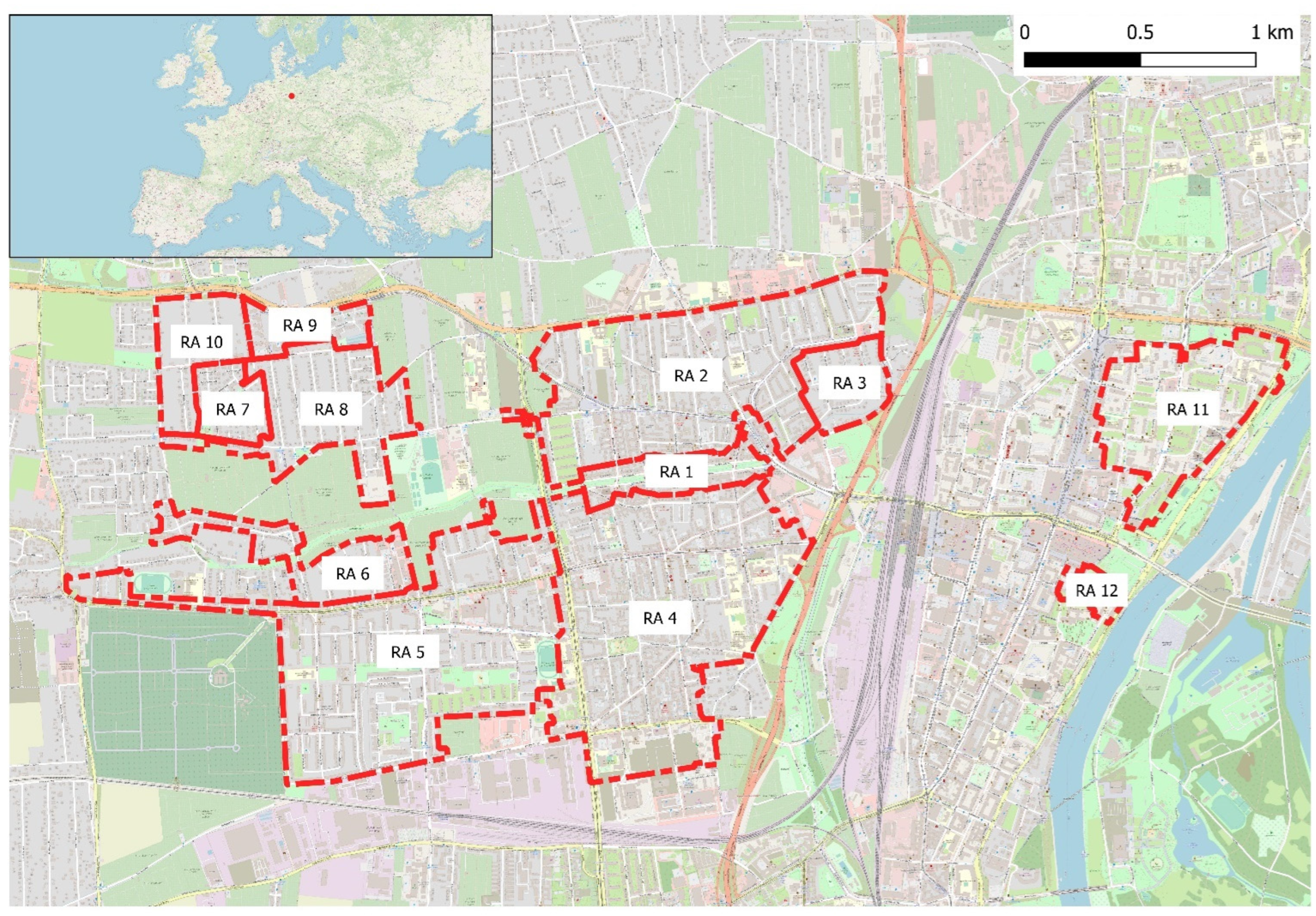
Figure 1. Areas of interest, City of Magdeburg. © https://www.openstreetmap.org and contributors.
Land 12 01725 g001
Figure 2. The relationship examined between the respective land use indicators.
Land 12 01725 g002
Figure 3. Methodological approach for the identification of linear relationships between the indicators under study; Note: the Kaiser–Meyer–Olkin criterion must have at least “mediocre” in min one of the regression methods (Spearman, Pearson, Kendall). Better scores (e.g., middling, meritorious) are explicitly desirable; the MSA must be greater or equal 0.5; the green arrows indicate the steps towards the result, and the red arrows indicate preparatory/corrective steps; the linkage of the initial data set with the regression results (to illustrate the effects) is symbolized with the black dashed arrow.
Land 12 01725 g003
Figure 4. Scree Plot of the PCA and FA result based on eigenvalue and factor or component number.
Land 12 01725 g004
Figure 5. Variable or indicator as Biplot for dimension 1 and 2.
Land 12 01725 g005
Figure 6. Variable or indicator as Biplot for dimension 3 and 4.
Land 12 01725 g006
Figure 7. Presentation of Model 1 (without adjustment) based on the standardized data for the corresponding residential areas (RAi, see Figure 1).
Land 12 01725 g007
Figure 8. Presentation of Model 1 (without adjustment) based on the back-transformed data for the corresponding residential areas in EUR per m2.
Land 12 01725 g008
Figure 9. Presentation of Model 2 (with linear Model fitting) based on the back-transformed data for the corresponding residential areas in EUR per m2.
Land 12 01725 g009
Figure 10. Presentation of Model 3 (with quadratic Model fitting) based on the back-transformed data for the corresponding residential areas in EUR per m2.
Land 12 01725 g010
Figure 11. Presentation of the Model comparison, based on the back-transformed data for the corresponding residential areas in EUR per m2.
Land 12 01725 g011
Figure 12. Presentation of the relationships between the number of street trees and standard land value. Explanation of the “difference of trees to the mean number of trees” (bar chart): increase in tree individuals compared to the mean (green), decrease in tree individuals compared to the mean (red).
Land 12 01725 g012
Figure 13. Presentation of the relationships between the number of street trees and standard land value with confidence interval.
Land 12 01725 g013
Figure 14. Presentation of the relationships between the distance to allotment gardens and standard land value. Explanation of the “difference of distance to the mean distance to allotments” (bar chart): increase in the distance to the nearest allotment garden compared to the mean (green), decrease in the distance to the nearest allotment garden compared to the mean (red).
Land 12 01725 g014
Figure 15. Presentation of the relationships between the distance to allotment gardens and standard land value with confidence interval.
Land 12 01725 g015
Figure 16. (A) Effect of trees for 2006, zero Model, 2020; (B) Effect of distance to allotments for 2006, zero Model, 2020 on the SLRV.
Land 12 01725 g016
Table 1. The district, with the corresponding residential areas with the entire areal area and green areas based on the normalized difference vegetation index NDVI.
DistrictResidential Area
j
Total Area in ha
ASLVR
Area of Green Spaces in ha
AGI
Stadtfeld OstRA 112.54.0
Stadtfeld OstRA 280.028.6
Stadtfeld OstRA 312.16.9
Stadtfeld OstRA 4102.230.0
Stadtfeld WestRA 598.647.8
Stadtfeld WestRA 618.69.4
Stadtfeld WestRA 79.75.5
Stadtfeld WestRA 832.119.5
Stadtfeld WestRA 98.74.6
Stadtfeld WestRA 1016.19.8
AltstadtRA 1138.715.3
AltstadtRA 124.11.8
Table 2. The test results for the MSA test with regression method Pearson for each indicator and iteration. Red = deleted variable, wavy undersigned = Indicator of Interest (<0.5); Italic: KMO value of the respective iteration.
Design.StartIter. 1Iter. 2Iter. 3Iter. 4Iter. 5Iter. 6Iter. 7Iter. 8
SLRV0.5770.6320.5680.5330.4640.5570.5640.5660.495
INH0.5180.5460.3820.3620.4630.6390.6330.6700.675
IMIG0.6550.5840.5050.4070.3210.5070.4450.483
OCR0.6770.5070.3910.2990.3990.5210.7400.7540.823
INC0.7040.6520.6700.6420.6070.5600.6020.5970.567
ISD0.6590.5450.6260.6000.6790.7570.7460.7420.733
IR0.6580.5700.5410.4780.5660.7070.6730.6630.650
Es0.2160.3680.2980.5650.3300.301
LAI0.2420.4060.2980.2380.284
Ntree0.2370.3270.4550.3200.5320.4270.4910.6290.663
GS0.5780.4610.4400.7740.5950.6080.5800.7910.733
BDI0.1990.145
AlG0.3230.5280.4510.3560.4890.6800.6480.5840.617
min_gi0.160
Water0.2090.3390.3240.2410.4030.4330.382
school0.2650.2740.2910.2610.5830.5680.5380.5630.561
min_med0.4710.3280.3290.2920.4580.6530.6420.5750.711
tra0.2670.2410.2410.203
ret0.3650.2110.163
rest_pkt0.3670.3440.4070.3260.4170.5310.6540.7480.803
KMO0.3740.4070.3950.3680.4660.5620.5950.6410.661
Table 3. PCA loadings with communality (h2), eigenvalue (EV), explained Variance (Var) and cumulative Variance (cum Var) after dimension reduction. Green highlight absolute charge > 0.5 & orange highlight absolute charge > 0.3.
DimensionDim.1Dim.2Dim.3h2
Indicator
SLRV−0.6730−0.39930.45780.8220
INH−0.77190.39240.04030.7515
OCR−0.3679−0.83880.00220.8390
INC−0.4715−0.8631−0.12300.9824
ISD0.45230.83460.14950.9235
IR−0.4588−0.8500−0.14820.9550
Ntree−0.49720.3709−0.66290.8242
GS0.7615−0.4143−0.06200.7554
AlG−0.67440.32580.27120.6345
school0.5361−0.33970.48510.6380
min_med0.7405−0.3764−0.18940.7258
rest_pkt0.7248−0.3704−0.10070.6727
EV4.463.991.07
Var37.20%33.26%8.91%
cum Var37.20%70.46%79.37%
Table 4. PCA loadings with communality (h2), eigenvalue (EV), explained Variance (Var) and cumulative Variance (cum Var). Green highlight absolute charge > 0.5 & orange highlight absolute charge > 0.3.
DimensionDim.1Dim.2Dim.3Dim.4Dim.5Dim.6Dim.7Dim.8Dim.9Dim.10Dim.11Dim.12h2
Indicator
SLRV−0.6730−0.39930.4578−0.0058−0.29390.00800.0352−0.29830.02460.0036−0.02110.01571.0000
INH−0.77190.39240.04030.38730.1722−0.1718−0.0620−0.0528−0.04810.10690.1378−0.00591.0000
OCR−0.3679−0.83880.0022−0.07320.2674−0.0219−0.1471−0.0268−0.23090.0186−0.08750.00071.0000
INC−0.4715−0.8631−0.12300.0240−0.04890.00970.0439−0.00240.0570−0.05460.0299−0.07421.0000
ISD0.45230.83460.1495−0.03050.0161−0.0024−0.0448−0.1286−0.1457−0.18010.0520−0.01981.0000
IR−0.4588−0.8500−0.14820.0245−0.00790.00640.03030.0911−0.0039−0.14350.11130.04551.0000
Es−0.49720.3709−0.66290.1879−0.24110.18310.1748−0.0631−0.11440.0191−0.02780.00301.0000
LAI0.7615−0.4143−0.0620−0.3806−0.02740.2441−0.0327−0.0894−0.05350.10700.1266−0.00261.0000
Ntree−0.67440.32580.2712−0.4759−0.0041−0.09890.32380.1273−0.08420.02530.0186−0.00551.0000
GI0.5361−0.33970.48510.5132−0.05390.20360.17820.1240−0.08280.01540.0016−0.00431.0000
AlG0.7405−0.3764−0.18940.09010.3126−0.17630.3209−0.18210.0318−0.0054−0.00860.00641.0000
school0.7248−0.3704−0.10070.0345−0.4206−0.3681−0.03640.0530−0.09170.03110.0130−0.00221.0000
EV4.463.991.070.840.530.340.300.200.120.080.060.01
Var37.20%33.26%8.91%6.97%4.39%2.84%2.53%1.64%1.00%0.68%0.50%0.07%
cum Var37.20%70.46%79.37%86.34%90.73%93.57%96.11%97.75%98.75%99.43%99.93%100.00%
Table 5. Results for multiple regression Model 1 (SLRV model basic; Equation (24)) r = 0.9192, adj. r2 = 0.8298, se = 0.4043.
VariableCoefficientenStandard
Error
t-Statisticp-ValueLower 95%Upper 95%
INH0.20770.05064.10190.00010.10770.3078
INC2.52860.195012.96700.00002.14322.9139
ISD0.62030.10545.88500.00000.41200.8286
IR−1.34720.1566−8.60400.0000−1.6566−1.0377
Ntree−0.18710.0430−4.35290.0000−0.2721−0.1022
AlG0.32550.04856.71300.00000.22970.4213
min_med−0.39280.0482−8.15070.0000−0.4881−0.2976
rest_pkt0.10950.05112.14390.03370.00860.2104
school0.26100.04425.90020.00000.17360.3484
Table 6. Results for multiple regression Model 2 Equation (25) r = 0.9192, adj. r2 = 0.8440, se = EUR 30.31 per m2.
VariableCoefficientenStandard
Error
t-Statisticp-ValueLower 95%Upper 95%
b90.99303.592625.32820.000083.896098.0901
m0.45750.015828.97340.00000.42630.4887
Table 7. Results for multiple regression Model 3 Equation (26) r = 0.9504, adj. r2 = 0.9019, se = EUR 24.03 per m2.
VariableCoefficientenStandard
Error
t-Statisticp-ValueLower 95%Upper 95%
b103.79183.145532.99710.000097.5776110.0060
m0.18440.03115.92930.00000.12300.2459
n0.00060.00019.59080.00000.00050.0008
Table 8. Basic data for the scenario development and model interpretation based on the “Zero Model”.
SLRV (Model 3)
EUR per m2
INH
Items per ha
School
m
INC
EUR per a
ISD
% per a
IR
%
Ntree
Items
AlG
m
min_med
m
rest_pkt
m
Mean152.6777504866,933,142,7691.310.6231421212237
Z0000000000
Disclaimer/Publisher’s Note: The statements, opinions and data contained in all publications are solely those of the individual author(s) and contributor(s) and not of MDPI and/or the editor(s). MDPI and/or the editor(s) disclaim responsibility for any injury to people or property resulting from any ideas, methods, instructions or products referred to in the content.

