


Indirect Prediction of Salt Affected Soil Indicator Properties through Habitat Types of a Natural Saline Grassland Using Unmanned Aerial Vehicle Imagery

 ,
,  , , , ,
Abstract
1. Introduction
2. Materials and Methods
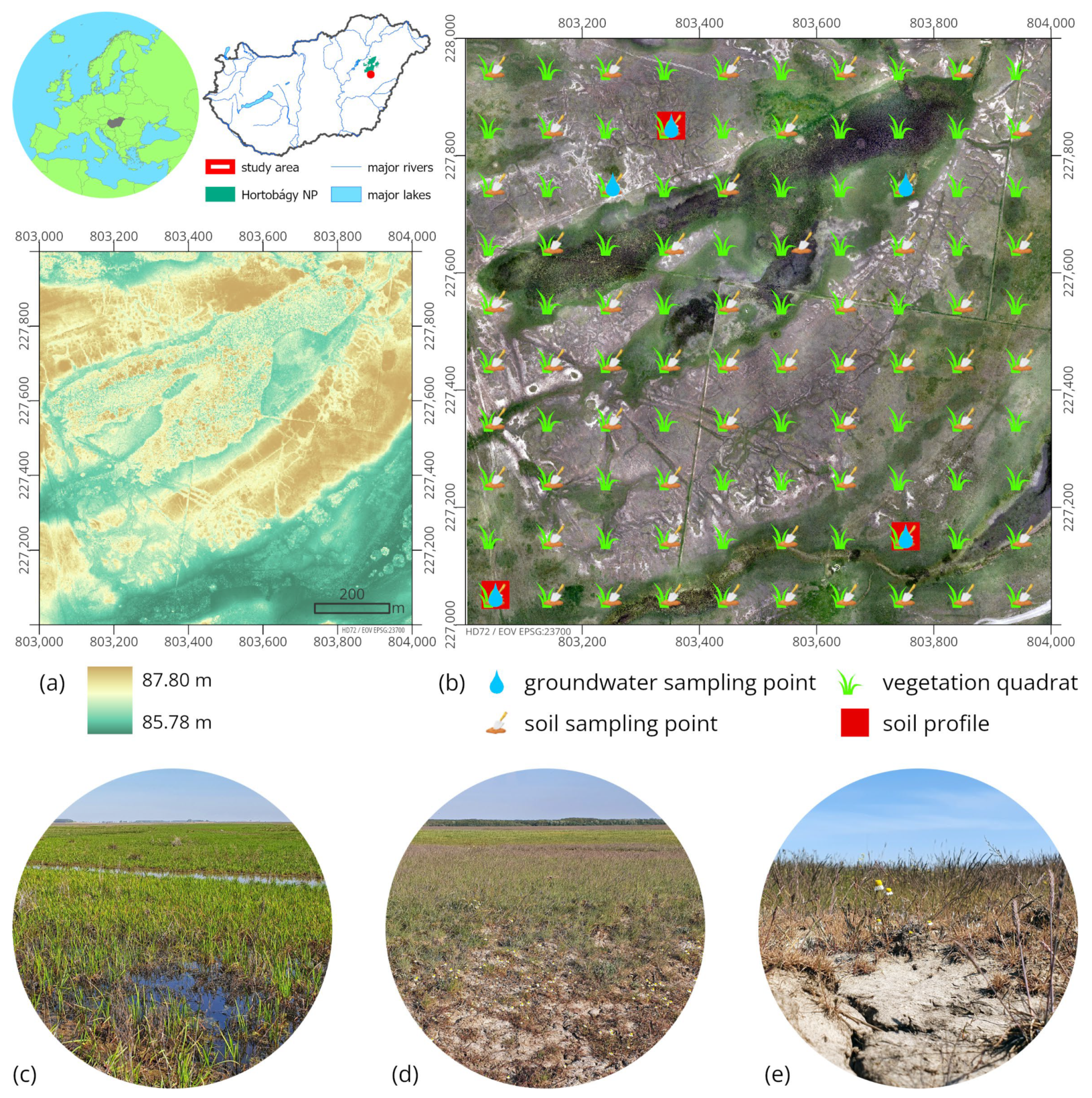
2.1. Study Site
2.2. Field Survey and Laboratory Analysis
2.2.1. Soil Sampling
2.2.2. Vegetation Survey
2.2.3. Proximal Soil Sensing
2.2.4. Laboratory Measurements
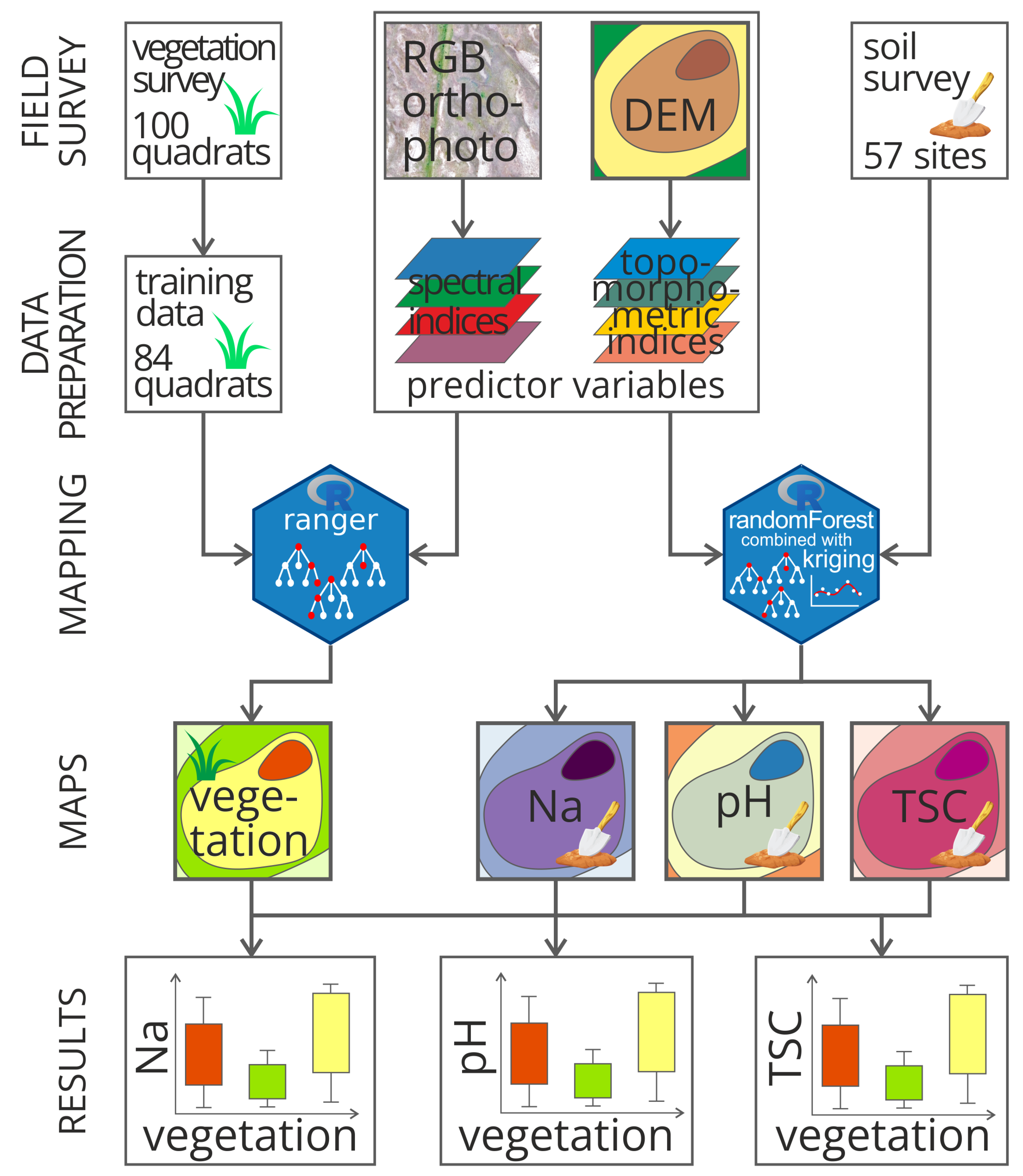
2.3. Methods
2.3.1. Vegetation Mapping
2.3.2. Spatial Modelling of Soil Properties
2.3.3. Validation of Soil Property Estimations
3. Results
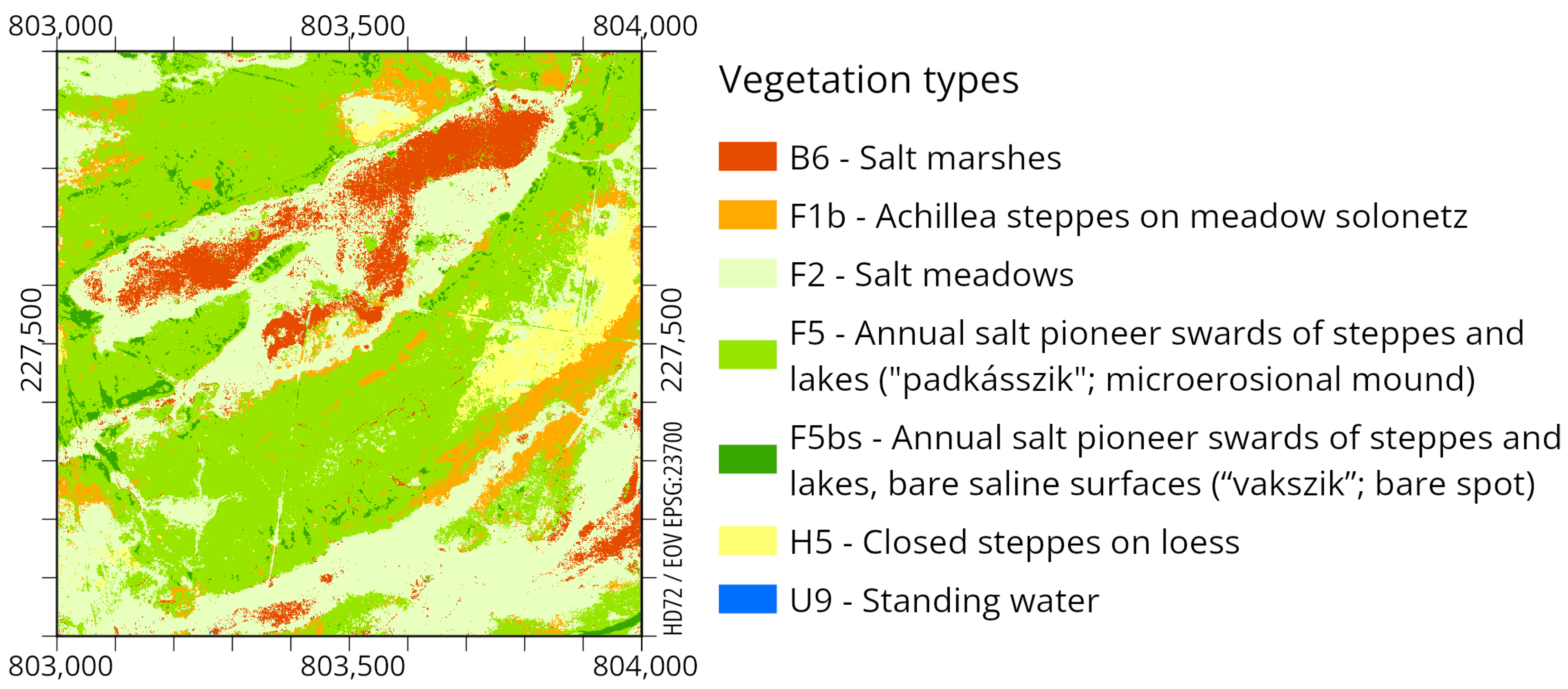
3.1. Vegetation Map
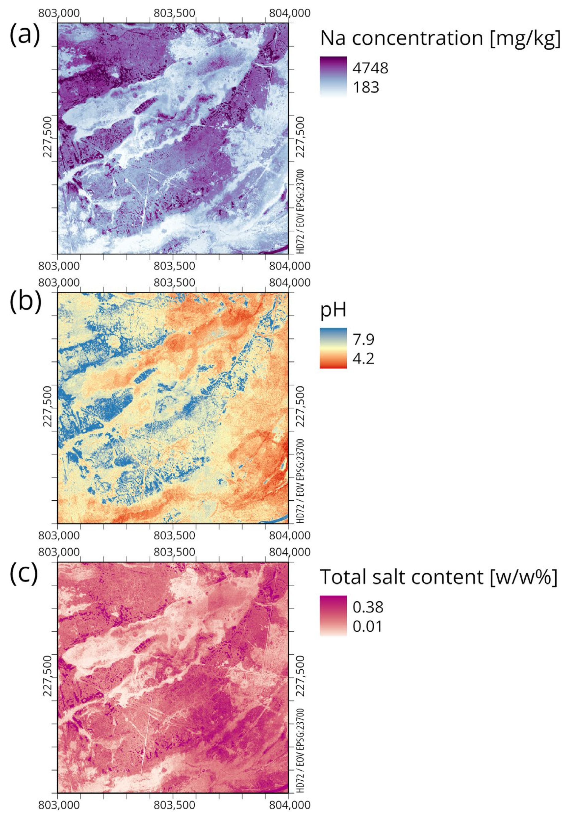
3.2. Thematic Soil Maps
4. Discussion
5. Conclusions
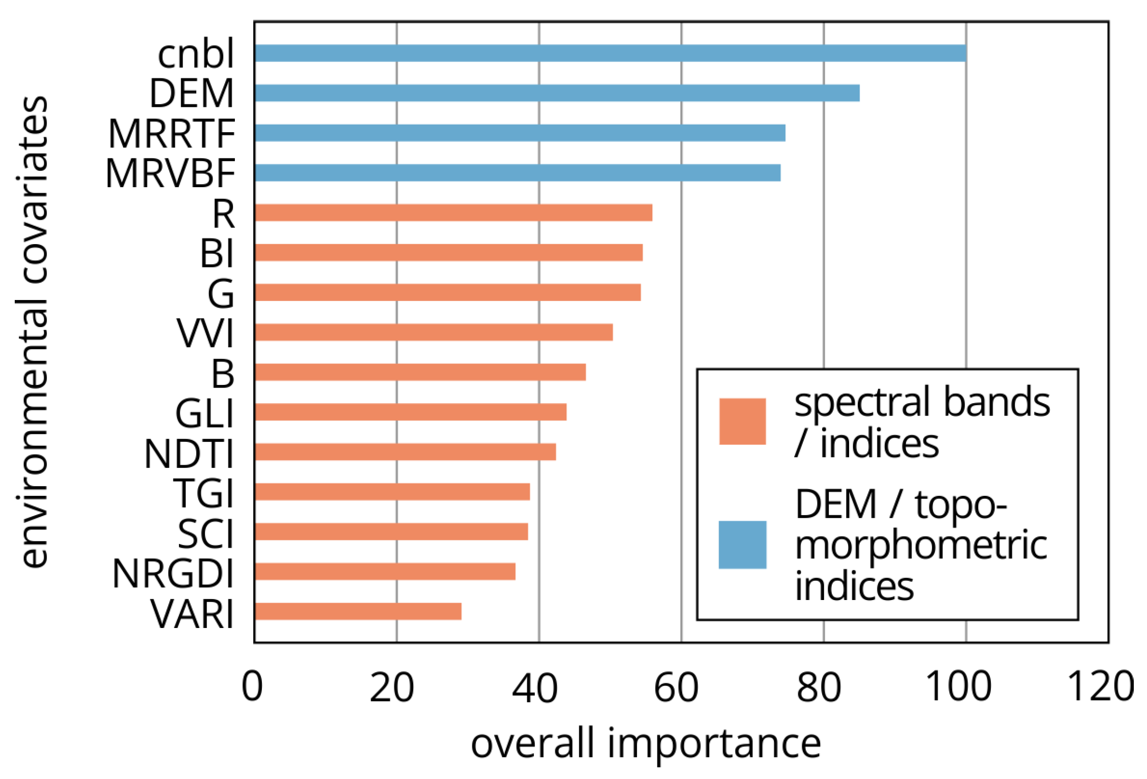
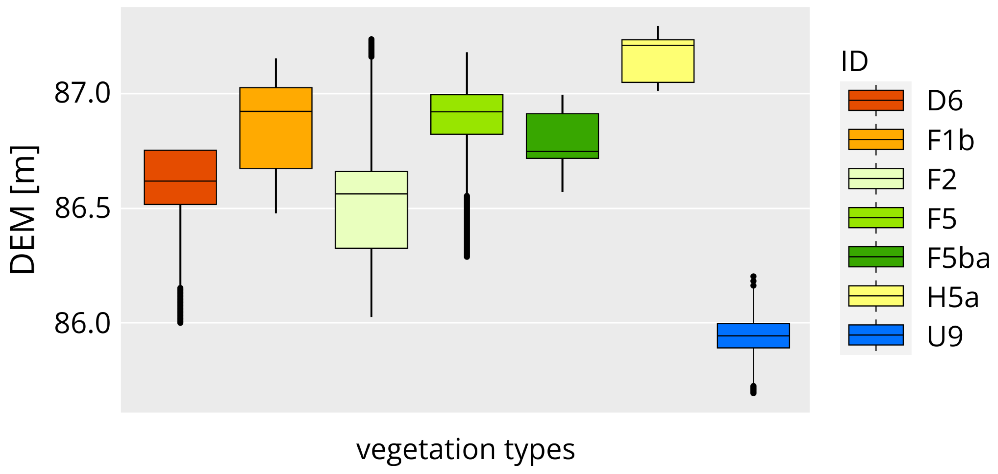
- The analysis of the classifier model’s (“ranger” machine learning) most important co-variables in case of preparing vegetation map, highlights the significance of morphometric variables (CNBL, DEM, MRRTF, and MRVBF) in the top four positions, followed by spectral variables (red, green, blue bands, BI, VVI, and GLI). Morphometric variables differentiate habitats based on altitude levels, while RGB bands and vegetation-related spectral indices separate different plant types. The BI is particularly useful in identifying bare spots with greyish-white surfaces. The applied geostatistical model demonstrated high accuracy (0.9889) and a Kappa value of 0.9857 when tested against the dataset. The classification performance for each habitat type was excellent, with balanced accuracy, precision, and recall values exceeding 0.95.
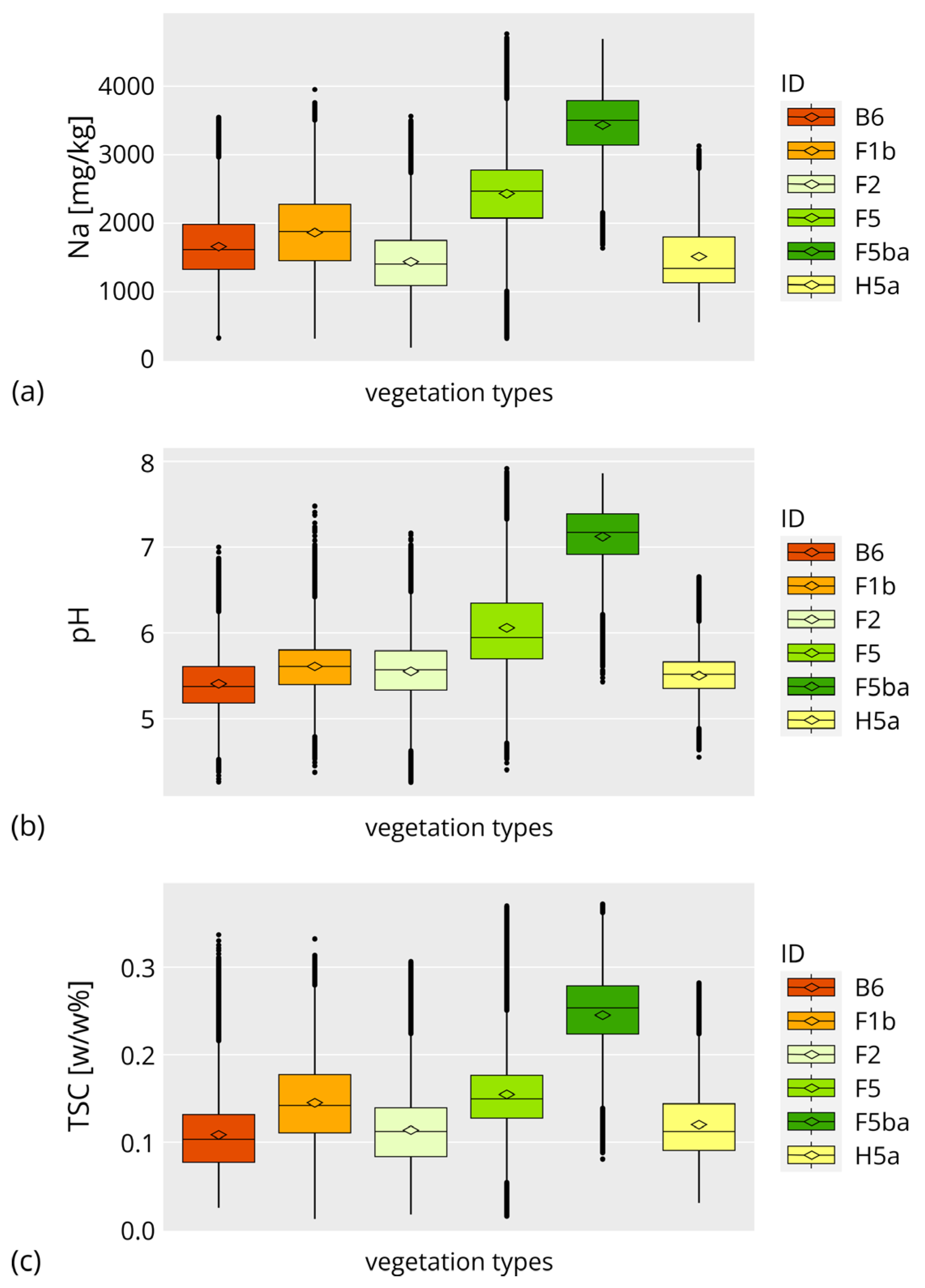
- Correlation analysis of thematic maps of SAS indicators (pH, Na, and TSC) and habitat map patterns was carried out applying boxplots. Our model-based estimation was successful to indirectly estimate these SAS indicators for every distinct habitat type, defining characteristic thresholds for the soil parameters.
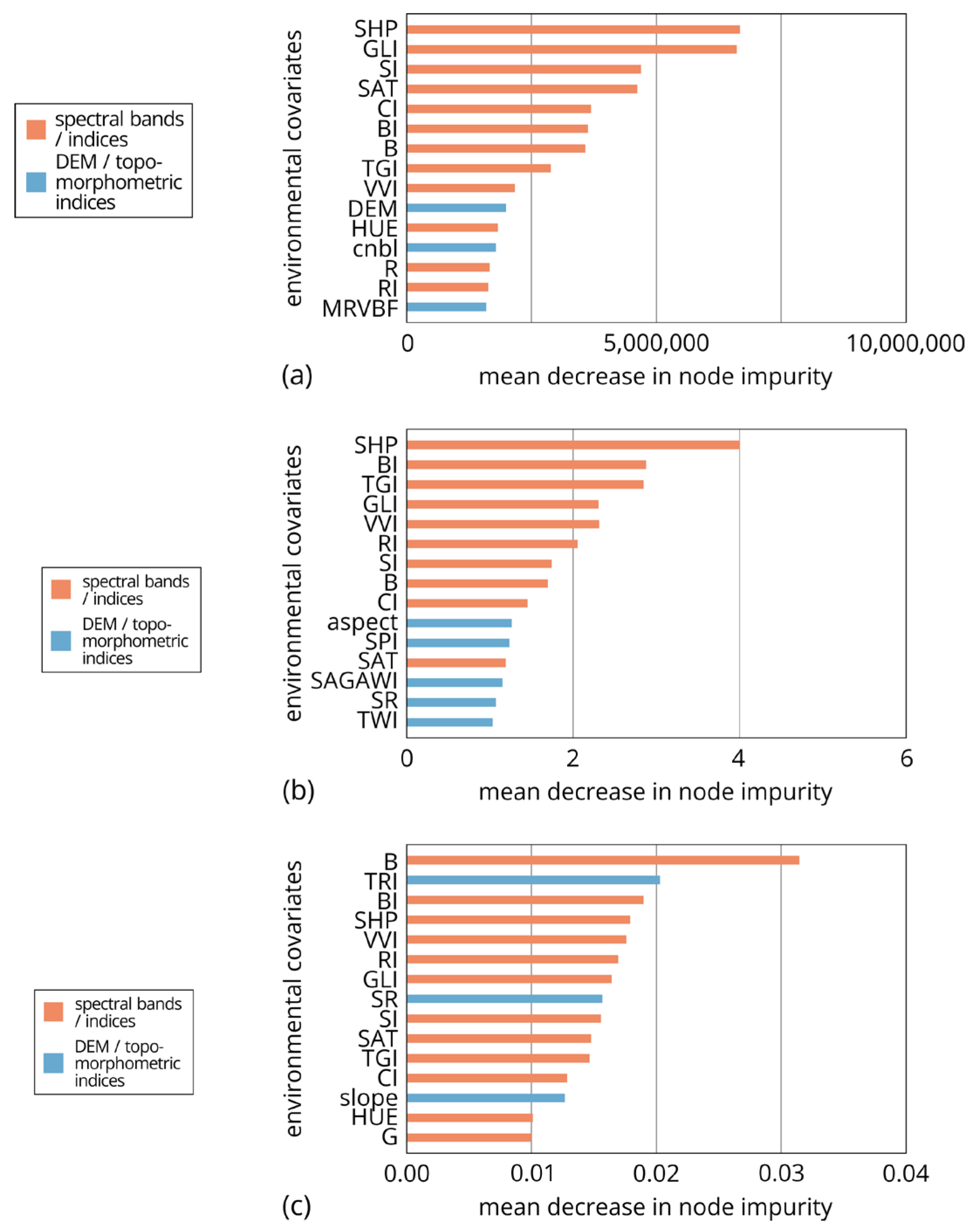
- For UAV-based RGB orthophotos, it was found that spectral indices (SHP, BI, TGI, GLI, VVI, RI, SI, B, CI, and SAT) provided more comprehensive information compared to topomorphometric indices when considering the importance of the variables in estimating all SAS parameters.
Supplementary Materials
Author Contributions
Funding
Data Availability Statement
Acknowledgments
Conflicts of Interest
References
- Montoroi, J.-P. Soil Salinization and Management of Salty Soils. In Soils as a Key Component of the Critical Zone 5: Degradation and Rehabilitation. Geosciences Series. Soils Set; Valenton, C., Ed.; ISTE, Wiley: London, UK, 2018; pp. 97–126. [Google Scholar]
- Zhao, M.; Wang, C.; He, Y.; He, T. Soil Characteristics and Response Thresholds of Salt Meadow on Lake Beaches of the Ordos Platform. Front. Environ. Sci. 2022, 10, 1050757. [Google Scholar] [CrossRef]
- Lubińska-Mielińska, S.; Kącki, Z.; Kamiński, D.; Pétillon, J.; Evers, C.; Piernik, A. Vegetation of Temperate Inland Salt-Marshes Reflects Local Environmental Conditions. Sci. Total Environ. 2023, 856, 159015. [Google Scholar] [CrossRef]
- IMEUH. Interpretation Manual of European Union Habitats; European Comission: Brussels, Belgium, 2007. [Google Scholar]
- Ladányi, Z.; Balog, K.; Tóth, T.; Barna, G. Longer-Term Monitoring of a Degrading Sodic Lake: Landscape Level Impacts of Hydrological Regime Changes and Restoration Interventions (SE Hungary). Arid. Land Res. Manag. 2023, 37, 389–407. [Google Scholar] [CrossRef]
- Eswar, D.; Karuppusamy, R.; Chellamuthu, S. Drivers of Soil Salinity and Their Correlation with Climate Change. Curr. Opin. Environ. Sustain. 2021, 50, 310–318. [Google Scholar] [CrossRef]
- Schofield, R.V.; Kirkby, M.J. Application of Salinization Indicators and Initial Development of Potential Global Soil Salinization Scenario under Climatic Change. Glob. Biogeochem. Cycles 2003, 17, 4-1–4-13. [Google Scholar] [CrossRef]
- McBratney, A.B.; Mendonça Santos, M.L.; Minasny, B. On Digital Soil Mapping. Geoderma 2003, 117, 3–52. [Google Scholar] [CrossRef]
- Minasny, B.; McBratney, A.B. Digital Soil Mapping: A Brief History and Some Lessons. Geoderma 2016, 264, 301–311. [Google Scholar] [CrossRef]
- Szatmári, G.; Bakacsi, Z.; Laborczi, A.; Petrik, O.; Pataki, R.; Tóth, T.; Pásztor, L. Elaborating Hungarian Segment of the Global Map of Salt-Affected Soils (GSSmap): National Contribution to an International Initiative. Remote Sens. 2020, 12, 4073. [Google Scholar] [CrossRef]
- Gorji, T.; Tanik, A.; Sertel, E. Soil Salinity Prediction, Monitoring and Mapping Using Modern Technologies. Procedia Earth Planet. Sci. 2015, 15, 507–512. [Google Scholar] [CrossRef]
- Suleymanov, A.; Gabbasova, I.; Komissarov, M.; Suleymanov, R.; Garipov, T.; Tuktarova, I.; Belan, L. Random Forest Modeling of Soil Properties in Saline Semi-Arid Areas. Agriculture 2023, 13, 976. [Google Scholar] [CrossRef]
- Keskin, H.; Grunwald, S. Regression Kriging as a Workhorse in the Digital Soil Mapper’s Toolbox. Geoderma 2018, 326, 22–41. [Google Scholar] [CrossRef]
- Szabó, B.; Szatmári, G.; Takács, K.; Laborczi, A.; Makó, A.; Rajkai, K.; Pásztor, L. Mapping Soil Hydraulic Properties Using Random-Forest-Based Pedotransfer Functions and Geostatistics. Hydrol. Earth Syst. Sci. 2019, 23, 2615–2635. [Google Scholar] [CrossRef]
- Nabiollahi, K.; Taghizadeh-Mehrjardi, R.; Shahabi, A.; Heung, B.; Amirian-Chakan, A.; Davari, M.; Scholten, T. Assessing Agricultural Salt-Affected Land Using Digital Soil Mapping and Hybridized Random Forests. Geoderma 2021, 385, 114858. [Google Scholar] [CrossRef]
- Heuvelink, G.B.M.; Webster, R. Spatial Statistics and Soil Mapping: A Blossoming Partnership under Pressure. Spat. Stat. 2022, 50, 100639. [Google Scholar] [CrossRef]
- Metternicht, G.I.; Zinck, J.A. Remote Sensing of Soil Salinity: Potentials and Constraints. Remote Sens. Environ. 2003, 85, 1–20. [Google Scholar] [CrossRef]
- Mulder, V.L.; de Bruin, S.; Schaepman, M.E.; Mayr, T.R. The Use of Remote Sensing in Soil and Terrain Mapping—A Review. Geoderma 2011, 162, 1–19. [Google Scholar] [CrossRef]
- Sahbeni, G.; Ngabire, M.; Musyimi, P.K.; Székely, B. Challenges and Opportunities in Remote Sensing for Soil Salinization Mapping and Monitoring: A Review. Remote Sens. 2023, 15, 2540. [Google Scholar] [CrossRef]
- Ivushkin, K.; Bartholomeus, H.; Bregt, A.K.; Pulatov, A.; Franceschini, M.H.D.; Kramer, H.; van Loo, E.N.; Jaramillo Roman, V.; Finkers, R. UAV Based Soil Salinity Assessment of Cropland. Geoderma 2019, 338, 502–512. [Google Scholar] [CrossRef]
- Richer-de-Forges, A.C.; Chen, Q.; Baghdadi, N.; Chen, S.; Gomez, C.; Jacquemoud, S.; Martelet, G.; Mulder, V.L.; Urbina-Salazar, D.; Vaudour, E.; et al. Remote Sensing Data for Digital Soil Mapping in French Research—A Review. Remote Sens. 2023, 15, 3070. [Google Scholar] [CrossRef]
- Dronova, I.; Kislik, C.; Dinh, Z.; Kelly, M. A Review of Unoccupied Aerial Vehicle Use in Wetland Applications: Emerging Opportunities in Approach, Technology, and Data. Drones 2021, 5, 45. [Google Scholar] [CrossRef]
- Lyu, X.; Li, X.; Dang, D.; Dou, H.; Wang, K.; Lou, A. Unmanned Aerial Vehicle (UAV) Remote Sensing in Grassland Ecosystem Monitoring: A Systematic Review. Remote Sens. 2022, 14, 1096. [Google Scholar] [CrossRef]
- Wang, Y.; Lu, Z.; Sheng, Y.; Zhou, Y. Remote Sensing Applications in Monitoring of Protected Areas. Remote Sens. 2020, 12, 1370. [Google Scholar] [CrossRef]
- Zhang, J.; Okin, G.S.; Zhou, B.; Karl, J.W. UAV-Derived Imagery for Vegetation Structure Estimation in Rangelands: Validation and Application. Ecosphere 2021, 12, e03830. [Google Scholar] [CrossRef]
- Zhang, H.; Feng, Y.; Guan, W.; Cao, X.; Li, Z.; Ding, J. Using Unmanned Aerial Vehicles to Quantify Spatial Patterns of Dominant Vegetation along an Elevation Gradient in the Typical Gobi Region in Xinjiang, Northwest China. Glob. Ecol. Conserv. 2021, 27, e01571. [Google Scholar] [CrossRef]
- Lehmann, J.R.K.; Prinz, T.; Ziller, S.R.; Thiele, J.; Heringer, G.; Meira-Neto, J.A.A.; Buttschardt, T.K. Open-Source Processing and Analysis of Aerial Imagery Acquired with a Low-Cost Unmanned Aerial System to Support Invasive Plant Management. Front. Environ. Sci. 2017, 5, 44. [Google Scholar] [CrossRef]
- Mustaffa, A.A.; Mukhtar, A.N.; Rasib, A.W.; Suhandri, H.F.; Bukari, S.M. Mapping of Peat Soil Physical Properties by Using Drone- Based Multispectral Vegetation Imagery. IOP Conf. Ser. Earth Environ. Sci. 2020, 498, 012021. [Google Scholar] [CrossRef]
- Oh, S.; Chang, A.; Yang, Y.E.; Kim, H.S.; Lim, K.J.; Jung, J. Recent Advances in UAS Based Soil Erosion Mapping. Mod. Concepts Dev. Agron. 2020, 7. [Google Scholar] [CrossRef]
- Takata, Y.; Yamada, H.; Kanuma, N.; Ise, Y.; Kanda, T. Digital Soil Mapping Using Drone Images and Machine Learning at the Sloping Vegetable Fields in Cool Highland in the Northern Kanto Region, Japan. Soil Sci. Plant Nutr. 2023, 69, 221–230. [Google Scholar] [CrossRef]
- Bertalan, L.; Holb, I.; Pataki, A.; Szabó, G.; Kupásné Szalóki, A.; Szabó, S. UAV-Based Multispectral and Thermal Cameras to Predict Soil Water Content—A Machine Learning Approach. Comput. Electron. Agric. 2022, 200, 107262. [Google Scholar] [CrossRef]
- Wei, G.; Li, Y.; Zhang, Z.; Chen, Y.; Chen, J.; Yao, Z.; Lao, C.; Chen, H. Estimation of Soil Salt Content by Combining UAV-Borne Multispectral Sensor and Machine Learning Algorithms. PeerJ 2020, 2020, e9087. [Google Scholar] [CrossRef] [PubMed]
- Ma, Y.; Zhu, W.; Zhang, Z.; Chen, H.; Zhao, G.; Liu, P. Fusion Level of Satellite and UAV Image Data for Soil Salinity Inversion in the Coastal Area of the Yellow River Delta. Int. J. Remote Sens. 2022, 43, 7039–7063. [Google Scholar] [CrossRef]
- Kahaer, Y.; Tashpolat, N. Estimating Salt Concentrations Based on Optimized Spectral Indices in Soils with Regional Heterogeneity. J. Spectrosc. 2019, 15, 2402749. [Google Scholar] [CrossRef]
- Silver, M.; Tiwari, A.; Karnieli, A. Identifying Vegetation in Arid Regions Using Object-Based Image Analysis with RGB-Only Aerial Imagery. Remote Sens. 2019, 11, 2308. [Google Scholar] [CrossRef]
- Last, W.M.; Ginn, F.M. Saline Systems of the Great Plains of Western Canada: An Overview of the Limnogeology and Paleolimnology. Saline Syst. 2005, 1, 10. [Google Scholar] [CrossRef] [PubMed]
- Dítě, D.; Šuvada, R.; Tóth, T.; Dítě, Z. Inventory of the Halophytes in Inland Central Europe. Preslia 2023, 95, 215–240. [Google Scholar] [CrossRef]
- Deák, B.; Valkó, O.; Alexander, C.; Mücke, W.; Kania, A.; Tamás, J.; Heilmeier, H. Fine-Scale Vertical Position as an Indicator of Vegetation in Alkali Grasslands—Case Study Based on Remotely Sensed Data. Flora-Morphol. Distrib. Funct. Ecol. Plants 2014, 209, 693–697. [Google Scholar] [CrossRef]
- Themistocleous, K. DEM Modeling Using RGB-Based Vegetation Indices from UAV Images. In Proceedings of the Seventh International Conference on Remote Sensing and Geoinformation of the Environment (RSCy2019), Paphos, Cyprus, 18–21 March 2019; Themistocleous, K., Papadavid, G., Michaelides, S., Ambrosia, V., Hadjimitsis, D., Eds.; SPIE: Bellingham, WA, USA, 2019; Volume 11174, pp. 499–506. [Google Scholar]
- Szatmári, G.; Pásztor, L. Comparison of Various Uncertainty Modelling Approaches Based on Geostatistics and Machine Learning Algorithms. Geoderma 2019, 337, 1329–1340. [Google Scholar] [CrossRef]
- Wang, L.; Wu, W.; Liu, H. Bin Digital Mapping of Topsoil PH by Random Forest with Residual Kriging (RFRK) in a Hilly Region. Soil Res. 2019, 57, 387–396. [Google Scholar] [CrossRef]
- Hengl, T.; Nussbaum, M.; Wright, M.N.; Heuvelink, G.B.M.; Gräler, B. Random Forest as a Generic Framework for Predictive Modeling of Spatial and Spatio-Temporal Variables. PeerJ 2018, 2018, e5518. [Google Scholar] [CrossRef]
- Dövényi, Z. (Ed.) Magyarország Kistájainak Katasztere [Inventory of Microregions in Hungary]; MTA Földrajztudományi Intézet: Budapest, Hungary, 2010. [Google Scholar]
- Novák, T.J.; Tóth, C.A. Development of Erosional Microforms and Soils on Semi-Natural and Anthropogenic Influenced Solonetzic Grasslands. Geomorphology 2016, 254, 121–129. [Google Scholar] [CrossRef]
- Tóth, C.; Novák, T.; Rakonczai, J. Hortobágy Puszta: Microtopography of Alkali Flats. In Landscapes and Landforms of Hungary; Lóczy, D., Ed.; Springer International Publishing: Cham, Switzerland, 2015; pp. 237–246. ISBN 978-3-319-08997-3. [Google Scholar]
- Tóth, T.; Szendrei, G. A Sókivirágzások Elterjedésének És Képződésének Összefüggése a Környezeti, Ezen Belül Talajtani Tényezőkkel [Relationship between Salt Efflorescences and Environmental Conditions with Special Emphasis on Edaphological Conditions]. Topogr. Mineral. Hung. 2006, IX, 79–90. [Google Scholar]
- Tóth, T.; Kuti, L. Összefüggés a Talaj Sótartalma És Egyes Földtani Tényezők Között a Hortobágyi “Nyírőlapos” Mintaterületen. I. Általános Földtani Jellemzés, a Felszín Alatti Rétegek Kalcittartalma És PH Értéke [Geological Factors Affecting the Salinization of the Nyírőlapos Sample Area (Hortobágy, Hungary). I. General Geological Characterization, Calcite Concentration and PH Values of Subsurface Layers]. Agrokémia Talajt. 1999, 48, 431–446. [Google Scholar]
- IUSS Working Group WRB. World Reference Base for Soil Resources 2014, Update 2015. World Soil Resources Reports 106; FAO: Rome, Italy, 2015. [Google Scholar]
- Michéli, E.; Fuchs, M.; Hegymegi, P.; Stefanovits, P. Classification of the Major Soils of Hungary and Their Correlation with the World Reference Base for Soil Resources (WRB). Agrokémia Talajt. 2006, 55, 19–28. [Google Scholar] [CrossRef]
- Gallai, B.; Árvai, M.; Mészáros, J.; Barna, G.; Pásztor, L.; Szatmári, G.; Ulicsni, V.; Tóth, B.; Novák, T.; Tóth, T. A Talaj És Növényzet Összefüggése a Hortobágyi Ágota-Pusztán [The Relationship between Soil and Vegetation Ágota-Puszta, Hortobágy]. In Proceedings of the Talajtani Vándorgyűlés, Sárvár, Hungary, 25 September 2020. [Google Scholar]
- Tóth, T.; Rajkai, K. Soil and Plant Correlations in a Solonetzic Grassland. Soil Sci. 1994, 157, 253–262. [Google Scholar] [CrossRef]
- Bölöni, J.; Molnár, Z.; Kun, A. (Eds.) Magyarország Élőhelyei. A Hazai Vegetációtípusok Leírása És Határozója. ÁNÉR 2011 [Habitats of Hungary]; MTA Ökológiai és Botanikai Kutatóintézete: Vácrátót, Hungary, 2011. [Google Scholar]
- Molnár, Z.; Biró, M.; Bölöni, J.; Horváth, F. Distribution of the (Semi-)Natural Habitats in Hungary I. Marshes and Grasslands. Acta Bot. Hung. 2009, 50, 59–105. [Google Scholar] [CrossRef]
- Reudenbach, C.; Meyer, H. UavRst R package: Unmanned Aerial Vehicle Remote Sensing Tools 2022. Available online: https://gisma.github.io/uavRst/ (accessed on 28 June 2023).
- Conrad, O.; Bechtel, B.; Bock, M.; Dietrich, H.; Fischer, E.; Gerlitz, L.; Wehberg, J.; Wichmann, V.; Böhner, J. System for Automated Geoscientific Analyses (SAGA) v. 2.1.4. Geosci. Model Dev. 2015, 8, 1991–2007. [Google Scholar] [CrossRef]
- Mohammadi, H.; Samadzadegan, F. An Object Based Framework for Building Change Analysis Using 2D and 3D Information of High Resolution Satellite Images. Adv. Space Res. 2020, 66, 1386–1404. [Google Scholar] [CrossRef]
- Gitelson, A.A.; Kaufman, Y.J.; Stark, R.; Rundquist, D. Novel Algorithms for Remote Estimation of Vegetation Fraction. Remote Sens. Environ. 2002, 80, 76–87. [Google Scholar] [CrossRef]
- Lacaux, J.P.; Tourre, Y.M.; Vignolles, C.; Ndione, J.A.; Lafaye, M. Classification of Ponds from High-Spatial Resolution Remote Sensing: Application to Rift Valley Fever Epidemics in Senegal. Remote Sens. Environ. 2007, 106, 66–74. [Google Scholar] [CrossRef]
- Madeira, J.; Bedidi, A.; Cervelle, B.; Pouget, M.; Flay, N. Visible Spectrometric Indices of Hematite (Hm) and Goethite (Gt) Content in Lateritic Soils: The Application of a Thematic Mapper (TM) Image for Soil-Mapping in Brasilia, Brazil. Int. J. Remote Sens. 1997, 18, 2835–2852. [Google Scholar] [CrossRef]
- Novák, J.; Lukas, V.; Kren, J. Estimation of Soil Properties Based on Soil Colour Index. Agric. Conspec. Sci. 2018, 83, 71–76. [Google Scholar]
- Mathieu, R.; Pouget, M.; Cervelle, B.; Escadafal, R. Relationships between Satellite-Based Radiometric Indices Simulated Using Laboratory Reflectance Data and Typic Soil Color of an Arid Environment. Remote Sens. Environ. 1998, 66, 17–28. [Google Scholar] [CrossRef]
- Raymond Hunt, E.; Daughtry, C.S.T.; Eitel, J.U.H.; Long, D.S. Remote Sensing Leaf Chlorophyll Content Using a Visible Band Index. Agron. J. 2011, 103, 1090–1099. [Google Scholar] [CrossRef]
- Louhaichi, M.; Borman, M.M.; Johnson, D.E. Spatially Located Platform and Aerial Photography for Documentation of Grazing Impacts on Wheat. Geocarto Int. 2001, 16, 65–70. [Google Scholar] [CrossRef]
- Tucker, C.J. Red and Photographic Infrared Linear Combinations for Monitoring Vegetation. Remote Sens. Environ. 1979, 8, 127–150. [Google Scholar] [CrossRef]
- Escadafal, R.; Belghit, A.; Ben-Moussa, A. Indices Spectraux Pour La Télédétection de La Dégradation Des Milieux Naturels En Tunisie Aride. In Proceedings of the Actes du 6eme Symposium International sur les Mesures Physiques et Signatures en Télédétection, Val d’Isère, France, 17–21 January 1994; pp. 253–259. [Google Scholar]
- Olaya, V. A Gentle Introduction to SAGA GIS. Available online: http://sourceforge.net/saga-gis/ (accessed on 28 June 2023).
- Wilson, J.; Gallant, J. Primary Topographic Attributes. In Terrain Analysis: Principles and Applications; Wilson, J., Gallant, J., Eds.; John Wiley & Sons, Inc.: Hoboken, NJ, USA, 2000; p. 520. [Google Scholar]
- Riley, S.; DeGloria, S.; Elliot, R. A Terrain Ruggeddness Index That Quantifies Topographic Heterogeneity. Int. J. Sci. 1999, 5, 23–27. [Google Scholar]
- Iwahashi, J.; Pike, R.J. Automated Classifications of Topography from DEMs by an Unsupervised Nested-Means Algorithm and a Three-Part Geometric Signature. Geomorphology 2007, 86, 409–440. [Google Scholar] [CrossRef]
- Olaya, V. Chapter 6 Basic Land-Surface Parameters. Dev. Soil Sci. 2009, 33, 141–169. [Google Scholar] [CrossRef]
- Böhner, J.; Selige, T. Spatial Prediction of Soil Attributes Using Terrain Analysis and Climate Regionalisation. In SAGA—Analysis and Modelling Applications. Göttinger Geographische Abhandlungen 115; Boehner, J., McCloy, K., Strobl, J., Eds.; Geographischen Instituts der Universität Göttingen: Göttingen, Germany, 2006; pp. 13–28. [Google Scholar]
- Böhner, J.; Antonić, O. Chapter 8 Land-Surface Parameters Specific to Topo-Climatology. Dev. Soil Sci. 2009, 33, 195–226. [Google Scholar] [CrossRef]
- Moore, I.D.; Grayson, R.B.; Ladson, A.R. Digital Terrain Modelling: A Review of Hydrological, Geomorphological, and Biological Applications. Hydrol. Process. 1991, 5, 3–30. [Google Scholar] [CrossRef]
- Friedrich, K. Multivariate Distance Methods for Geomorphographic Relief Classification. In Land Inforamtion Systems—Developments for Planning the Sustainable Use of Land Resources. European Soil Bureau—Research Report 4, EUR 17729 EN; Heinecke, H., Eckelmann, W., Thomasson, A., Jones, J., Montanarella, L., Buckley, B., Eds.; Office for Oficial Publications of the European Communities: Ispra, Italy, 1998; pp. 259–266. [Google Scholar]
- Gallant, J.C.; Dowling, T.I. A Multiresolution Index of Valley Bottom Flatness for Mapping Depositional Areas. Water Resour. Res. 2003, 39, 1347. [Google Scholar] [CrossRef]
- Beven, K.J.; Kirkby, M.J. A Physically Based, Variable Contributing Area Model of Basin Hydrology. Hydrol. Sci. Bull. 1979, 24, 43–69. [Google Scholar] [CrossRef]
- Ayers, R.S.; Westcot, D.W. Water Quality for Agriculture. FAO Irrigation and Drainage Paper 29 Rev. 1; FAO: Rome, Italy, 1985. [Google Scholar]
- Wright, M.N.; Ziegler, A. Ranger: A Fast Implementation of Random Forests for High Dimensional Data in C++ and R. J. Stat. Softw. 2017, 77, 1–17. [Google Scholar] [CrossRef]
- Kuhn, M. Building Predictive Models in R Using the Caret Package. J. Stat. Softw. 2008, 28, 1–26. [Google Scholar] [CrossRef]
- Breiman, L. Random Forests. Mach. Learn. 2001, 45, 5–32. [Google Scholar] [CrossRef]
- Hengl, T.; MacMillan, R.A. Predictive Soil Mapping with R; OpenGeoHub Foundation: Wageningen, The Netherlands, 2019. [Google Scholar]
- Hengl, T. A Practical Guide to Geostatistical Mapping of Environmental Variables. EUR 22904 EN; Office for Official Publications of the European Communities: Luxembourg, 2007; ISBN 978-92-79-06904-8. [Google Scholar]
- Šefferová Stanová, V.; Janák, M.; Ripka, J. Management of Natura 2000 Habitats. 1530 *Pannonic Salt Steppes and Salt Marshes; Technical Report; European Comission: Brussels, Belgium, 2008; Available online: https://ec.europa.eu/environment/nature/natura2000/management/habitats/pdf/1530_Pannonic_salt_steppes.pdf (accessed on 28 June 2023).
- Elnaggar, A.A.; Noller, J.S. Application of Remote-Sensing Data and Decision-Tree Analysis to Mapping Salt-Affected Soils over Large Areas. Remote Sens. 2009, 2, 151–165. [Google Scholar] [CrossRef]
- Zhang, Z.; Niu, B.; Li, X.; Kang, X.; Hu, Z. Estimation and Dynamic Analysis of Soil Salinity Based on UAV and Sentinel-2A Multispectral Imagery in the Coastal Area, China. Land 2022, 11, 2307. [Google Scholar] [CrossRef]
- Zhao, W.; Zhou, C.; Zhou, C.; Ma, H.; Wang, Z. Soil Salinity Inversion Model of Oasis in Arid Area Based on UAV Multispectral Remote Sensing. Remote Sens. 2022, 14, 1804. [Google Scholar] [CrossRef]
- Tóth, T.; Csillag, F.; Biehl, L.L.; Michéli, E. Characterization of Semivegetated Salt-Affected Soils by Means of Field Remote Sensing. Remote Sens. Environ. 1991, 37, 167–180. [Google Scholar] [CrossRef]
- Mougenot, B.; Pouget, M. Remote Sensing of Salt Affected Soils. Remote Sens. Rev. 1993, 7, 241–259. [Google Scholar] [CrossRef]
- Tóth, T.; Kertész, M.; Pásztor, L. New Approaches in Salinity/Sodicity Mapping in Hungary. Agrokémia Talajt. 1998, 47, 76–86. [Google Scholar]
- Farifteh, J.; Farshad, A.; George, R.J. Assessing Salt-Affected Soils Using Remote Sensing, Solute Modelling, and Geophysics. Geoderma 2006, 130, 191–206. [Google Scholar] [CrossRef]
- Jamali, A.A.; Montazeri Naeeni, M.A.; Zarei, G. Assessing the Expansion of Saline Lands through Vegetation and Wetland Loss Using Remote Sensing and GIS. Remote Sens. Appl. 2020, 20, 100428. [Google Scholar] [CrossRef]
- Benos, L.; Tagarakis, A.C.; Dolias, G.; Berruto, R.; Kateris, D.; Bochtis, D. Machine Learning in Agriculture: A Comprehensive Updated Review. Sensors 2021, 21, 3758. [Google Scholar] [CrossRef]
- García-Fernández, M.; Sanz-Ablanedo, E.; Rodríguez-Pérez, J.R. High-Resolution Drone-Acquired RGB Imagery to Estimate Spatial Grape Quality Variability. Agronomy 2021, 11, 655. [Google Scholar] [CrossRef]
- Fu, Z.; Yu, S.; Zhang, J.; Xi, H.; Gao, Y.; Lu, R.; Zheng, H.; Zhu, Y.; Cao, W.; Liu, X. Combining UAV Multispectral Imagery and Ecological Factors to Estimate Leaf Nitrogen and Grain Protein Content of Wheat. Eur. J. Agron. 2022, 132, 126405. [Google Scholar] [CrossRef]
- Li, Z.; Zhou, X.; Cheng, Q.; Fei, S.; Chen, Z. A Machine-Learning Model Based on the Fusion of Spectral and Textural Features from UAV Multi-Sensors to Analyse the Total Nitrogen Content in Winter Wheat. Remote Sens. 2023, 15, 2152. [Google Scholar] [CrossRef]
- Yamamoto, S.; Nomoto, S.; Hashimoto, N.; Maki, M.; Hongo, C.; Shiraiwa, T.; Homma, K. Monitoring Spatial and Time-Series Variations in Red Crown Rot Damage of Soybean in Farmer Fields Based on UAV Remote Sensing. Plant Prod. Sci. 2023, 26, 36–47. [Google Scholar] [CrossRef]
- Sahbeni, G. Prediction of Soil Salinity Using a Random Forest-Based Model between 2000 and 2016. A Case Study in the Great Hungarian Plain. In Proceedings of the Global Symposium on Salt-Affected Soils, online, 20–22 October 2021. [Google Scholar]
- Hateffard, F.; Balog, K.; Tóth, T.; Mészáros, J.; Árvai, M.; Kovács, Z.A.; Szűcs-Vásárhelyi, N.; Koós, S.; László, P.; Novák, T.J.; et al. High-Resolution Mapping and Assessment of Salt-Affectedness on Arable Lands by the Combination of Ensemble Learning and Multivariate Geostatistics. Agronomy 2022, 12, 1858. [Google Scholar] [CrossRef]
- Dajic-Stevanovic, Z.; Pecinar, I.; Kresovic, M.; Vrbnicanin, S.; Tomovic, L. Biodiversity, Utilization and Management of Grasslands of Salt Affected Soils in Serbia. Community Ecol. 2008, 9, 107–114. [Google Scholar] [CrossRef]
- Szabolcs, I.; Rédly, M. State and Possibilities of Soil Salinization in Europe. Agrokémia Talajt. 1989, 38, 537–558. [Google Scholar]
- Szabolcs, I.; Máté, F. A Hortobágyi Szikes Talajok Genetikájának Kérdéséhez. [On the Genesis of Alkaline Soils of Hortobágy]. Agrokémia Talajt. 1955, 4, 31–38. [Google Scholar]
- Kovda, V.A. Origin of Saline Soils and Their Regime I; USSR Academy of Sciences: Moscow, Russia, 1946. (In Russian) [Google Scholar]
- Kovda, V. Origin of Saline Soils and Their Regime II; USSR Academy of Sciences: Moscow, Russia, 1947. (In Russian) [Google Scholar]
- Várallyay, G. Extreme Moisture Regime as the Main Limiting Factor of the Fertility of Salt Affected Soils. Agrokémia Talajt. 1981, 30, 73–96. [Google Scholar]
- Wagenet, R.J.; Jury, W.A. Movement and Accumulation of Salts in Soils. In Soil Salinity under Irrigation. Ecological Studies; Shainberg, I., Shalhevet, J., Eds.; Springer: Berlin/Heidelberg, Germany, 1984; Volume 51, pp. 100–129. [Google Scholar]
- Szabolcs, I.; Várallyay, G.; Darab, K. Soil and Hydrologic Surveys for the Prognosis and Monitoring of Salinity and Alkalinity. In Proceedings of the Prognosis of Salinity and Alkalinity. Report of an Expert Consultation, Rome, Italy, 3–6 June 1975; FAO Soil Bulletin 31. FAO: Rome, Italy, 1976; pp. 119–130. [Google Scholar]
- Várallyay, G. Environmental Stresses Induced by Salinity/Alkalinity in the Carpathian Basin (Central Europe). Agrokémia Talajt. 2004, 51, 233–242. [Google Scholar] [CrossRef]
- Dítě, Z.; Šuvada, R.; Tóth, T.; Jun, P.E.; Píš, V.; Dítě, D. Current Condition of Pannonic Salt Steppes at Their Distribution Limit: What Do Indicator Species Reveal about Habitat Quality? Plants 2021, 10, 530. [Google Scholar] [CrossRef]
- Csontos, P.; Tamás, J.; Kovács, Z.; Schellenberger, J.; Penksza, K.; Szili-Kovács, T.; Kalapos, T. Vegetation Dynamics in a Loess Grassland: Plant Traits Indicate Stability Based on Species Presence, but Directional Change When Cover Is Considered. Plants 2022, 11, 763. [Google Scholar] [CrossRef] [PubMed]
- Molnár, Z. Ősi És Másodlagos Eredetű Tiszántúli Szikes Puszták Zonációja [Zonation of Primary and Secondary Solonetz Alkaline Steppes in the Crisicum (Pannonicum)]. Acta Biol. Debrecina. Suppl. Oecol. Hung. 2010, 22, 181–189. [Google Scholar]
- Kertész, M.; Tóth, T. Soil Survey Based on Sampling Scheme Adjusted to Local Heterogeneity. Agrokémia Talajt. 1994, 43, 113–132. [Google Scholar]
- Steven, M.; Malthus, T.; Danson, F.; Jaggard, K.; Andrieu, B. Monitoring Response of Vegetation to Stress. In Proceedings of the Proceedings Remote Sensing Society Annual Conference, Dundee, UK, 15–17 September 1992; pp. 369–377. [Google Scholar]
- Tóth, T. Salt-Affected Soils and Their Native Vegetation in Hungary. In Sabkha Ecosystems: Volume III: Africa and Southern Europe; Öztürk, M., Böer, B., Barth, H.-J., Clüsener-Godt, M., Khan, M.A., Breckle, S.-W., Eds.; Springer: Dordrecht, The Netherlands, 2011; pp. 113–132. ISBN 978-90-481-9673-9. [Google Scholar]


| Habitat Code | Description of Habitat Type | Note |
|---|---|---|
| B6 | Salt marshes | |
| F1b | Achillea steppes on Meadow solonetz | |
| F2 | Salt meadows | |
| F5 | Annual salt pioneer swards of steppes and lakes | “padkásszik” (microerosional mound) |
| F5bs 1 | Annual salt pioneer swards of steppes and lakes | “vakszik” (bare spot) |
| H5a | Closed steppes on loess | |
| U9 | Standing waters |
| Environmental Co-Variable | Reference | |
|---|---|---|
| Spectral indices | Red band (R) | |
| Green band (G) | ||
| Blue band (B) | ||
| Visible Vegetation Index (VVI) | [56] | |
| Visible Atmospherically Resistant Index (VARI) | [57] | |
| Normalized Difference Turbidity Index (NDTI) | [58] | |
| Redness Index (RI) | [59] | |
| Soil Color Index (SCI) | [60] | |
| Brightness Index (BI) | [61] | |
| Spectral Slope Saturation Index (SI) | [61] | |
| Hue Index (HI) | [61] | |
| Triangular Greeness Index (TGI) | [62] | |
| Green Leaf Index (GLI) | [63] | |
| Normalized Green Red Difference Index (NGRDI) | [64] | |
| Green Leaf Area Index (GLAI) | [54] | |
| Overall Hue Index (HUE) | [65] | |
| Coloration Index (CI) | [65] | |
| Overall Saturation Index (SAT) | [65] | |
| Shape Index (SHP) | [65] | |
| Topomorphometric indices | DEM | |
| Slope | [66] | |
| Aspect | [66] | |
| Topographic Position Index (TPI) | [67] | |
| Terrain Ruggeddness Index (TRI) | [68] | |
| Surface roughness (SR) | [69] | |
| Flow direction (flowdir) | [70] | |
| Catchment area (carea) | [70] | |
| Modified catchment area (mcarea) | [71] | |
| General curvature (GC) | [70] | |
| Diurnal anisotropic heating (DAH) | [72] | |
| LS factor (LS) | [73] | |
| Mass Balance Index (MBI) | [74] | |
| Multi-resolution Ridge Top Flatness (MRRTF) | [75] | |
| Multi-resolution Valley Bottom Flatness (MRVBF) | [75] | |
| Real Surface Area (RSA) | [66] | |
| Stream Power Index (SPI) | [73] | |
| SAGA Wetness Index (SAGAWI) | [71] | |
| Vertical distance to channel network (vd2cn) | [66] | |
| Channel network base level (cnbl) | [66] | |
| Topographic Wetness Index (TWI) | [76] |
| Hungarian Standard of the Measurement | Parameter | Unit | Instrument | Accuracy | Nr. of Data |
|---|---|---|---|---|---|
| MSZ 1484-22:2009 (Note 1) | pH of groundwater | - | Multi Line P4, WTW Multi 350i, Xylem Analytics Germany Sales GmbH & Co. KG, WTW, Weilheim, Germany | 0.004 | 5 |
| MSZ EN 27888:1998 (Note2) | Electrical conductivity of groundwater | dS/m | Multi Line P4, WTW Multi 350i, Xylem Analytics Germany Sales GmbH & Co. KG, WTW, Weilheim, Germany | 1 µS/cm | 5 |
| MSZ 1484-3:2006 (Note 3) | Calcium and Magnesium ion concentration of ground water | mg/L | Ultima-2 type ICP OES, Horiba Jobin Yvon SAS., Longjumeau, France | 0.5 µg/L | 5 |
| MSZ 1484-3:2006 (Note 3) | Sodium and Potassium ion concentration of groundwater | mg/L | Ultima-2 type ICP OES, Horiba Jobin Yvon SAS, Longjumeau, France | 0.5 (Mg), 1.0 (Na) µg/L | 5 |
| MSZ-08-0206-2:1978, 2.1 section (Note 4) | Reaction of the soil | pH | Radelkis OP-300, Radelkis Elektroanalitikai Műszergyártó Kft, Budapest, Hungary, digital pH measuring device, Sentron Europe B.V., Leek, The Netherlands | ±0.05 | 57 |
| MSZ-08-0206-2:1978, 2.4 section (Note 4) | Total salt content of soil | w/w% | Radelkis OK-102/1 conductometer, Radelkis Elektroanalitikai Műszergyártó Kft, Budapest, Hungary | 5–7.5 rel.% | 57 |
| MSZ 20135:1999, 5.1 (Note 5) | Na concentration of soil | mg/kg | iCAP 7400 ICP-OES Analyzer Thermo Scientific Duo View, Thermo Fisher Scientific (Praha) s.r.o., Praha, Czech republic | 4–7.5 rel.% | 57 |
| Habitat Code | Area (m2) | Percent (%) |
|---|---|---|
| B6 | 82,825.25 | 8.28 |
| F1b | 102,861.25 | 10.29 |
| F2 | 314,694.75 | 31.47 |
| F5 | 439,985.75 | 44.00 |
| F5bs | 24,518.50 | 2.45 |
| H5a | 34,991.75 | 3.50 |
| U9 | 122.75 | 0.01 |
| Delete Column | Na | pH | TSC | |
|---|---|---|---|---|
| ME | 19.10 | 0.03 | −0.00 | |
| RMSE | 971.45 | 0.88 | 0.09 |
| Habitat Types | Á-NÉR Codes | TSC (w/w%) | Na (mg/kg) | pH | |||
|---|---|---|---|---|---|---|---|
| Threshold | |||||||
| Low | High | Low | High | Low | High | ||
| Salt marshes | B6 | 0.08 | 0.13 | 1322.74 | 1976.77 | 5.18 | 5.60 |
| Achillea steppes on Meadow solonetz | F1b | 0.11 | 0.18 | 1444.19 | 2264.35 | 5.40 | 5.80 |
| Salt meadow | F2 | 0.08 | 0.14 | 1085.91 | 1747.34 | 5.32 | 5.79 |
| Annual salt pioneer swards of steppes and lakes (microerosional mound) | F5 | 0.13 | 0.18 | 2067.34 | 2763.57 | 5.69 | 6.34 |
| Annual salt pioneer swards of steppes and lakes (bare spot) | F5bs | 0.22 | 0.28 | 3126.08 | 3776.23 | 6.91 | 7.39 |
| Closed steppes on loess | H5a | 0.09 | 0.14 | 1128.18 | 1793.46 | 5.35 | 5.66 |
| Standing waters | U9 | 0.09 | 0.15 | 861.18 | 1639.39 | 4.86 | 5.45 |
Disclaimer/Publisher’s Note: The statements, opinions and data contained in all publications are solely those of the individual author(s) and contributor(s) and not of MDPI and/or the editor(s). MDPI and/or the editor(s) disclaim responsibility for any injury to people or property resulting from any ideas, methods, instructions or products referred to in the content. |
© 2023 by the authors. Licensee MDPI, Basel, Switzerland. This article is an open access article distributed under the terms and conditions of the Creative Commons Attribution (CC BY) license (https://creativecommons.org/licenses/by/4.0/).
Share and Cite
Pásztor, L.; Takács, K.; Mészáros, J.; Szatmári, G.; Árvai, M.; Tóth, T.; Barna, G.; Koós, S.; Kovács, Z.A.; László, P.; et al. Indirect Prediction of Salt Affected Soil Indicator Properties through Habitat Types of a Natural Saline Grassland Using Unmanned Aerial Vehicle Imagery. Land 2023, 12, 1516. https://doi.org/10.3390/land12081516
Pásztor L, Takács K, Mészáros J, Szatmári G, Árvai M, Tóth T, Barna G, Koós S, Kovács ZA, László P, et al. Indirect Prediction of Salt Affected Soil Indicator Properties through Habitat Types of a Natural Saline Grassland Using Unmanned Aerial Vehicle Imagery. Land. 2023; 12(8):1516. https://doi.org/10.3390/land12081516
Chicago/Turabian StylePásztor, László, Katalin Takács, János Mészáros, Gábor Szatmári, Mátyás Árvai, Tibor Tóth, Gyöngyi Barna, Sándor Koós, Zsófia Adrienn Kovács, Péter László, and et al. 2023. "Indirect Prediction of Salt Affected Soil Indicator Properties through Habitat Types of a Natural Saline Grassland Using Unmanned Aerial Vehicle Imagery" Land 12, no. 8: 1516. https://doi.org/10.3390/land12081516
APA StylePásztor, L., Takács, K., Mészáros, J., Szatmári, G., Árvai, M., Tóth, T., Barna, G., Koós, S., Kovács, Z. A., László, P., & Balog, K. (2023). Indirect Prediction of Salt Affected Soil Indicator Properties through Habitat Types of a Natural Saline Grassland Using Unmanned Aerial Vehicle Imagery. Land, 12(8), 1516. https://doi.org/10.3390/land12081516