Article

Demonstrating the Use of the Yield-Gap Concept on Crop Model Calibration in Data-Poor Regions: An Application to CERES-Wheat Crop Model in Greece

by
Melpomeni Nikou
1,2 and
Theodoros Mavromatis
1,*
1
Department of Meteorology and Climatology, School of Geology, Aristotle University of Thessaloniki, 541 24 Thessaloniki, Greece
2
Soil and Water Resources Institute, Hellenic Agricultural Organization (H.A.O.)—“DEMETER”, 570 01 Thessaloniki, Greece
*
Author to whom correspondence should be addressed.
Land 2023, 12(7), 1372; https://doi.org/10.3390/land12071372
Submission received: 8 June 2023 / Revised: 3 July 2023 / Accepted: 6 July 2023 / Published: 8 July 2023

Abstract

:
Yield estimations at global or regional spatial scales have been compromised due to poor crop model calibration. A methodology for estimating the genetic parameters related to grain growth and yield for the CERES-Wheat crop model is proposed based on yield gap concept, the GLUE coefficient estimator, and the global yield gap atlas (GYGA). Yield trials with three durum wheat cultivars in an experimental farm in northern Greece from 2004 to 2010 were used. The calibration strategy conducted with CERES-Wheat (embedded in DSSAT v.4.7.5) on potential mode taking into account the year-to-year variability of relative yield gap Yrg (YgC_adj) was: (i) more effective than using the average site value of Yrg (YgC_unadj) only (the relative RMSE ranged from 10 to 13% for the YgC_adj vs. 48 to 57% for YgC_unadj) and (ii) superior (slightly inferior) to the strategy conducted with DSSAT v.4.7.5 (DSSAT v.3.5—relative RMSE of 5 to 8% were found) on rainfed mode. Earlier anthesis, maturity, and decreased potential yield (from 2.2 to 3.9% for 2021–2050, and from 5.0 to 7.1% for 2071–2100), due to increased temperature and solar radiation, were found using an ensemble of 11 EURO-CORDEX regional climate model simulations. In conclusion, the proposed strategy provides a scientifically robust guideline for crop model calibration that minimizes input requirements due to operating the crop model on potential mode. Further testing of this methodology is required with different plants, crop models, and environments.

1. Introduction

Crop models are collections of mathematical equations that represent the various processes occurring within the plant and the interactions between the plant and its environment [1]. They have become indispensable tools in decision making, especially for future crop performance projections and impact studies under varied conditions (e.g., [2,3]). Before their reliable use in crop model applications, however, the challenging but essential process of calibration is required. Calibration is undertaken in many fields that use process-based models and involves adjusting model parameters to reduce the error between the model results and the measured data [4]. A constant challenge with crop model calibration is the unavailability of reliable input data on weather, soil, and crop management. Approaches that identified the most scientifically robust requirements for data availability and quality, as well as other, less rigorous options when data are not available or are of poor quality, were recently proposed [3,5]. Software used for the calibration is an additional concern. Often one ‘externally’ couples the existing model software to calibration software (e.g., [6]), but this can require substantial effort. As a result, calibration for crop models is often performed by manual trial and error, a time-consuming process that likely ends in a non-optimal solution, especially if several parameters are estimated, and it cannot be replicated without using an automated routine [7]. This, however, could also be a deliberate choice to exert more supervision over the calibration process. A further uncertainty with calibration is the errors observed data might have [4].
Yield trials are experiments in several environments (site-year combinations) with which a set of cultivars is usually assessed to make genotype recommendations [8]. Although they are labor intensive, time consuming, and expensive [9], they usually provide only yield measurements, ordinarily replicated, for several genotypes grown in various environments. In addition, these measurements are rather noisy (the standard deviation of plot yields exceeds 25% of the mean) and may not provide input information in space and time needed for crop model calibration [10]. Due to shortcomings of yield trials, a crop model’s calibration can be hindered by data limitations, even if a suitable model is chosen [3]. These challenges further increase in areas with Mediterranean climate (such as Greece), which is characterized by unfavorable growth conditions (particularly for rainfed crops such as wheat) caused by water stress coupled with low soil fertility and/or poor agronomic practices.
Cultivar characteristics should ideally be defined on potential production level (i.e., the crop growth rate) and thus yield is determined only by solar radiation, temperature, atmospheric CO2, and crop characteristics, and is not limited by water supply and nutrients. As a result, while potential yield is location-specific (depends on the local climate), it is not soil-specific [11] (more discussion in Section 2.2).
While many studies that use crop simulation models assessing crop yield gaps in different applications with concerns associated with data sources and methods (including poor quality of weather and soil data, unrealistic assumptions about the cropping-system context, poorly calibrated crop simulation models, and lack of transparency about underpinning assumptions and methods (e.g., [11]) have been published during the past decades [5], there is no published study that uses the yield-gap concept to facilitate with calibrating crop models. Since poorly tested crop models can seriously distort a study’s results, decreasing their usefulness to inform regional or national policies and effective prioritization of research and development investments for agriculture (e.g., [5]), there is an urgent need for an approach that will allow the determination of genotype’s characteristics required by crop models and minimize the required data from field experiments.
In this context, a methodology based on the concept of yield gap is developed to estimate the required by the crop model CERES-Wheat genetic parameters for grain growth and yield and minimize the numerous input data (e.g., site-specific initial soil moisture conditions) required. The GLUE coefficient estimator (see Section 2.2.2 for more specifics) was used for this purpose. The results of this methodology are compared with these of a traditional calibration strategy using data from yield trials, for three durum wheat cultivars, collected from the Aristotle University Farm in Thessaloniki, Greece, during 2004 to 2010. Finally, sensitivity analysis of wheat development and yield with CERES-Wheat based on climate change projections from an ensemble of 11 EURO-CORDEX regional climate model (RCM) simulations (see Section 2.2.5 for more specifics), under the influence of the moderate mitigation emission scenario RCP4.5 for the future periods 2021–2050 (near future) and 2071–2100 (the-end-of-the-century), was also conducted.

2. Materials and Methods

2.1. Yield Trials

Yield trials for three durum wheat cultivars (Mexicali, Sifnos, and Simeto) were conducted at the farm of the Cereal Institute (40°31′ N; 23°00′ E; 15 m altitude) of Thermi, in Thessaloniki, Greece, during 2004–2010 (Figure 1). The experiments (9 for Mexicali and 10 for Sifnos and Simeto) were carried out in four replicates using the randomized full block (RCBD) design. The experimental designs were of two sizes and covered areas of 7 and 14 m2, respectively. The varieties studied were plots of the experimental fields of the institute. Each experimental plot consisted of seven plant lines. The distance between the rows was 25 cm. The seed rate used was 180 kg/ha. Sowing was carried out on different dates from mid-November to the end of December, while planting depth ranged from 3 to 5 cm. In each experimental plot, ploughing with a plough and fine soil tillage with a disc harrow were carried out before sowing. Basic fertilization (80 kg/ha) was applied to all experimental fields using 20-10-10 fertilizer. Also, a top dressing (40 kg/ha) was applied to the experimental fields using 20-0-0 fertilizer. A second surface fertilization (20 kg/ha, 20-0-0) and plant protection products for weed control (Topik 240 EC for grasses and Brominal for broadleaves) were applied to some of the experimental plots.
Soil surface parameters such as soil pH, organic carbon, nitrogen, cation exchange capacity, and bulk density were estimated in Soil Science Institute of Thessaloniki [12]. Albedo and drainage rate were determined based on by Jones et al. (1986) [13] and Suleiman and Ritchie (2001) [14], respectively. Soil physical properties such as the lower limit of soil water content, the water content at the drained-upper limit, the saturation water content, and the saturated hydraulic conductivity, were estimated at the Land Improvement Institute of Thessaloniki. Emergence date, end ear growth date, and final grain yield were all observed. In 2009–10, physiology maturity date, grain counts, and individual grain weight were also collected. Phosphorous and nitrogen applied to all treatment. Diseases, weeds, and pest infestations were controlled. More details regarding the experiments can be found in Symeonidis (2011) [12].

2.2. Methods

2.2.1. The CERES-Wheat Crop Model

The CERES-Wheat crop model, embedded in the Decision Support System for Agrotechnology Transfer (DSSAT v. 4.7.5) [15,16], simulates wheat growth, development, and yield considering the effects of weather, genetics, soil (water, carbon, and nitrogen), planting, irrigation, and nitrogen fertilizer management through simulated water and nutrient limitations to plant growth (e.g., [3]). The model is designed to have applicability in diverse environments and to utilize a minimum data set of field and weather data as input. Daily solar radiation, maximum and minimum air temperature, and precipitation were collected from the site’s meteorological station. These variables are used to calculate potential reference evaporation and the CO2 transpiration feedback. It has been reported that CERES-Wheat successfully simulates wheat growth and yield in response to management and environmental factors across a wide range of soil and climate conditions (e.g., [12,17,18,19]).

2.2.2. The GLUE Coefficient Estimator

During calibration of CERES-Wheat, the genetic parameters that influence phenology, grain growth, and yield were determined by employing the GLUE coefficient estimator [6]. The GLUE is a popular Bayesian method [20,21,22]. Its main principle is to discretize parameter space by generating a large amount of parameter values from an approximate discrete prior distribution using Bayes’ equation. According to this, probability values are associated with the corresponding parameter combinations set each time [6,20]. The greater the probability, the higher the chance that its combination is the desired one. There is no exact inverse solution for large models with numerous parameters. Therefore, more than one set of genetic parameters could be selected to optimize a goodness-of-fit criterion given the observations [23]. Section 3.2 elaborates on the methodology used for the selection of genetic parameters in this study.

2.2.3. Estimating Genetic Parameters for CERES-Wheat

To simulate wheat development, growth, and yield, CERES-Wheat requires a set of seven cultivar specific genetic parameters (Table 1). These represent various physiological processes and growth parameters of the wheat plant.

Coefficients Related to Crop Development

P1V and P1D play important roles in determining timing of anthesis and maturity in wheat. Anthesis is the stage when the wheat plant produces flowers, and maturity is when the plant reaches physiological maturity and stops accumulating dry matter. P1V is the number of days required for optimum vernalizing temperature to complete vernalization, a critical step in wheat development that affects the timing of flowering and maturity. P1D, on the other hand, represents the percentage reduction in development rate in a photoperiod 10 h shorter than the threshold relative to the development rate at the threshold. Accurate estimation of P1D is important for simulating duration of the vegetative and reproductive phases of wheat development, which can affect the timing of anthesis and maturity. P5 determines the duration of the grain-filling phase in wheat. This phase is critical for final grain yield as it contributes to grain size and weight [24]. Longer grain-filling periods generally lead to larger, more mature grains and higher yields. However, if the period is too long, the plants may become over-mature, leading to reduced quality and yields. Accurate determination of P5 is therefore essential for predicting crop maturity and optimizing grain yield. Finally, PHINT represents the interval between successive leaf tip appearances and is an indicator of the rate of crop development. Accurate estimation of PHINT can help simulate the overall growth rate of the plant, including the timing of anthesis and maturity [16,17,25].
First, the P1V and P1D parameters were adjusted to match the observed anthesis dates observed during 2004 and 2010 using the GLUE method. Afterwards, the grain-filling phase duration (P5 parameter) was determined so that the simulated maturity of 2009–10 coincided with the observed one. This thermal requirement was assumed unchanged for all simulations since physiological maturity was not systematically observed in the yield trials.

Coefficients Related to Crop Yield

G1, G2, and G3 are important genetic parameters affecting wheat yield potential (Table 1). G1, the kernel number per unit canopy weight at anthesis, is an important determinant of grain yield in wheat. Accurate determination of G2, the standard kernel size under optimum conditions, can help in simulating the optimal kernel size for wheat. G3, the standard non-stressed dry weight of a single tiller at maturity, influences the final grain yield through its contribution on the optimal biomass accumulation [15,16,26].
G1, G2, and G3 were adjusted after fitting of development stages (anthesis and maturity), using the GLUE method, to match the observed grain yield, during 2004–2010 as suggested by literature (e.g., [16,27]). CERES-Wheat was run in three different ways: (a) in potential mode, accounting for the year-to-year variability of the relative yield gap Yrg (ΥgC_adj); (b) in potential mode, using an average site value of Yrg (therefore, the year-to-year variability of Yrg was not accounted (ΥgC_unadj)); and (c) in rainfed mode, with simulated water and nitrogen stresses and making the same assumptions for initial soil moisture and planting of each growing season with these of Symeonidis (2011) [12] (TrC). Finally, GLUE was used to match observed grain yield by adjusting G3 and PHINT (the interval between successive leaf tip appearances), since the latter parameter was found to influence both phenological development and yield [28].

2.2.4. Calibration Strategies

This study proposes a procedure based on yield gap analysis (YgC) to overcome the limitations of traditional calibration (TrC) in rainfed environments.

Calibration Based on Yield Gap Analysis (YgC)

Although cultivar characteristics should ideally be defined on a potential production level, where yield is determined only by crop characteristics, climate, and no limitations imposed by water supply and nutrients [11], they are traditionally estimated, even for rainfed crops, based on crop observations and measurements made under water and/or nitrogen stress conditions (i.e., water- and/or nutrient-limited production level). As a result, during crop model calibration, the limiting effects of water and nutrient stresses (deficits or excesses) on crop development and particularly on growth (the degree depends the severity and duration of the water and nutrient stresses) reflect on the estimation of the genetic parameters related mainly to grain and growth characteristics. To overcome a problematic calibration procedure leading to distorted genetic parameters (e.g., [12,17,18,19]), a procedure based on yield gap analysis (YgC) is proposed in this study. According to this, the crop model is run on potential mode, and the simulated yield for each year i (Yp(i)) was then adjusted by the relative yield gap (Yrg(i)) to achieve agreement with the actual, for the specific year i, harvested yield (Yac(i)):
Y r g i = Y g i Y s p i × 100
where the yield gap (Yg(i)) is defined as the difference between the yield potential for a specific location and time (Ysp(i)) and the actual farm yield (Yac(i)) [5,29]. Yg is a crucial biophysical indication of the available room for crop production increase with current land and water resources. The maximum yield of a crop cultivar grown in an environment to which it is adapted, with water and nutrient availability unlimited, and with pests, diseases, weeds, lodging, and other stresses effectively controlled, is known as potential site yield Ysp (also called yield potential) [30]. Actual yield Yac is the yield obtained with the available resources and the farmers’ current practices as determined from an area’s and a crop’s production data for a specific district and time frame [31]. At least four methods were proposed to estimate yield gaps at a local level (see Section 4 for more discussion): (1) field experiments, (2) yield contests, (3) maximum farmer yields based on surveys, and (4) crop model simulations [11].
In this study, the site- and year-specific Yrg(i) values from the global yield gap atlas (GYGA) [32,33] were used. The WOFOST crop model [34] was used for their estimation, as described by Van Ittersum et al. (2013) [11]. The major processes incorporated in WOFOST are temperature-dependent phenological development, CO2 assimilation, transpiration, respiration, partitioning of assimilates to the various organs, and yield formation (under potential and water/nutrient-limited conditions) [35]. The skills of WOFOST in simulating wheat phenology and yield have been extensively tested across Europe [36].

Traditional Calibration (TrC)

The initial soil water conditions of the experiments under consideration, which the crop model requires to operate in rainfed mode, were unknown. To overcome this restriction, it was assumed that the soil profile would be full on the first wet day (a day with prec > 0.1 mm) before planting for all experiments (this constitutes the traditional calibration strategy (TrC) in this study). This is a common assumption when initial soil water information is missing. It is reminded that the crop model assumes that soils are homogeneous and isotropic horizontally, layered vertically, with free drainage at the lower boundary. To facilitate strategy comparison, the assumptions made in TrC regarding initial soil moisture conditions in the planting of each growing season were these used by Symeonidis (2011) [12] with DSSAT v.3.5: (i) for the first 15 cm of soil, its moisture was calculated to match plant emergence in the field, (ii) for depths below 15 cm, CERES-Wheat was used to calculate moisture conditions before each growing period throughout dormancy, starting from a dry sequence to reach the limit of permanent wilting point, and (iii) the maximum root depth was assumed to be 60 cm.

2.2.5. Sensitivity Analysis

Sensitivity of wheat development and yield to climate change was conducted by using an ensemble of 11 high-resolution regional climate model (RCM) simulations (Table S1) of 12.5 km spatial resolution from the EURO-CORDEX project [37,38], which provide climate change projections for the moderate Representative Concentration Pathway (RCP4.5). The number in the name of the scenario refers to the radiative forcing caused by changes in the composition of the atmosphere at the end of the century. According to the RCP4.5 scenario, greenhouse gas emissions will decrease over time starting from 2040. The study covered the historical period from 1981 to 2005 along with the future periods 2021 to 2050 (the near future, NF) and 2071–2100 (the end-of-the-century, EOC) for the RCP4.5 emission scenario. Daily precipitation, solar radiation, and maximum and minimum air temperature data were utilized from those simulations. About temperature, a statistically significant increase is expected in NF by 1.5–2.0 °C compared to the reference period (1971–2000) over the wider Greek territory in mountainous parts for RCP4.5. At the end of the century, it is expected that coastal areas will witness a temperature increase of 2.0–2.5 °C. On the other hand, the analysis of precipitation indicates no statistically significant changes, with some areas facing an increase and others a decrease [39].

2.2.6. Statistical Measures

Several statistical measures were used to evaluate the relationship between predicted and observed wheat development and yield. These included the coefficient of determination (R2), which expresses the degree of collinearity between predicted and observed data, ranging from 0 to 1 (0.0 to 0.09: little (very weak) if any fit; 0.09 to 0.25: low (weak) fit; 0.25 to 0.49: moderate fit; 0.49 to 0.81: high (strong) fit; 0.81 to 1.0 very high (very strong) fit [40]). Mean absolute error (MAE), mean bias error (MBE), and root mean squared error (RMSE) were also estimated as follows:
M A E = i = 1 n P i O i n
M B E = i = 1 n P i O i n
R M S E = i = 1 n P i O i 2 n
where n is the number of observations, Pi is the model predictions, and Oi is the observed value, for year i. Regression analysis was also applied to evaluate the calibration strategies.

3. Results

3.1. Yield Gap Analysis

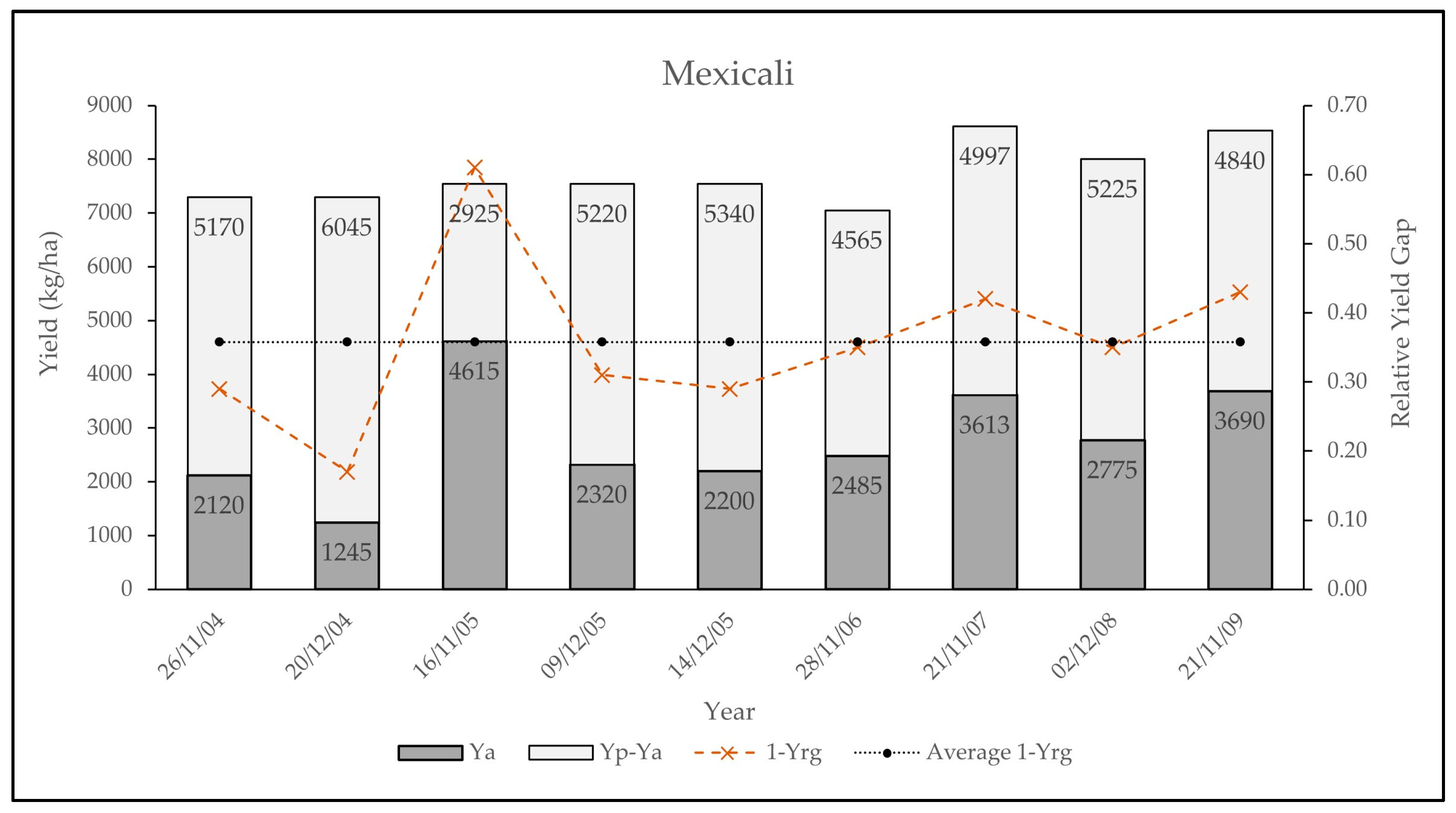
The actual wheat yield (Ya) for Thermi ranged from 1.2 t/ha for 2004 to 4.8 t/ha for 2005, with the three cultivars exhibiting similar variability (34–35% when expressed in terms of coefficient of variation (std/mean × 100)). The correlation between the cultivars is also very high (from 96% to 98%). The potential yield (Yp) from the global yield gap atlas varied from 7.0 t/ha for 2007 to 8.6 t/ha for 2008 for the three cultivars (Figure 2 and Figure S1). The higher Yp was observed in 2007 and the lower in 2006. The correlation between actual and potential yield is 0.72 for Simeto and 0.55 for Mexicali and Sifnos. The yield gaps (Yp-Ya) between actual and potential yield for the specific yield trials ranged from 2.9 t/ha to 6.0 t/ha for Mexicali, from 2.7 t/ha to 6.1 t/ha for Sifnos and from 3.4 t/ha to 6.1 t/ha for Simeto. The higher relative yield gaps (1-Yrg) × 100 (%) occurred in 2005 early plantings for both cultivars (61% for Mexicali, 64% for Sifnos and 55% for Simeto), and the lower in 2004 late plantings (17% for Mexicali and 16% for both Sifnos and Simeto), which also coincided with the higher and the lower Ya, respectively, for the three cultivars.

3.2. Selection of Genetic Coefficients

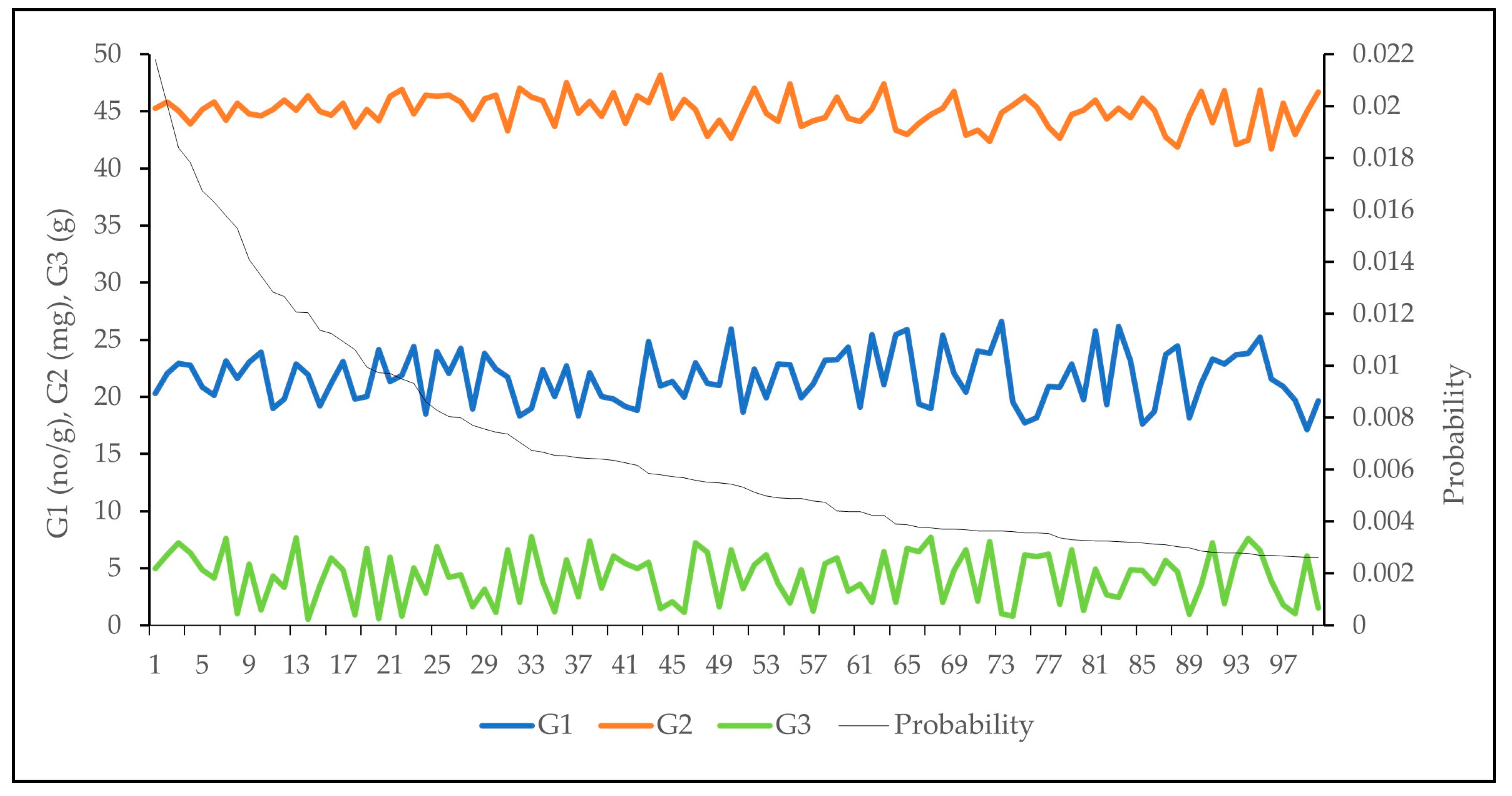
Choosing genetic parameters is usually made based on the statistical measure that is considered more useful with respect to application purposes [41]. In this study, the selection of genetic parameters was not only based on the probability given by GLUE but also on MAE and RMSE. In the case of fitting measured yield, for example, GLUE was used to identify the parameters G1, G2, and G3 to fit measured yield, and from the 9000 of combinations tested, 100 along with their corresponding probabilities, arranged from highest to lowest probability, are shown for Mexicali in Figure 3. The values for G1 ranged from 17.1 to 26.6 (no/g), for G2 from 41.7 to 48.2 (mg) and for G3 from 0.5 to 7.7 (g), with the last parameter showing the largest variability (51.8% for G3 vs. 10.5% for G1 and 3.1% for G2%) when expressed in terms of coefficient of variation.
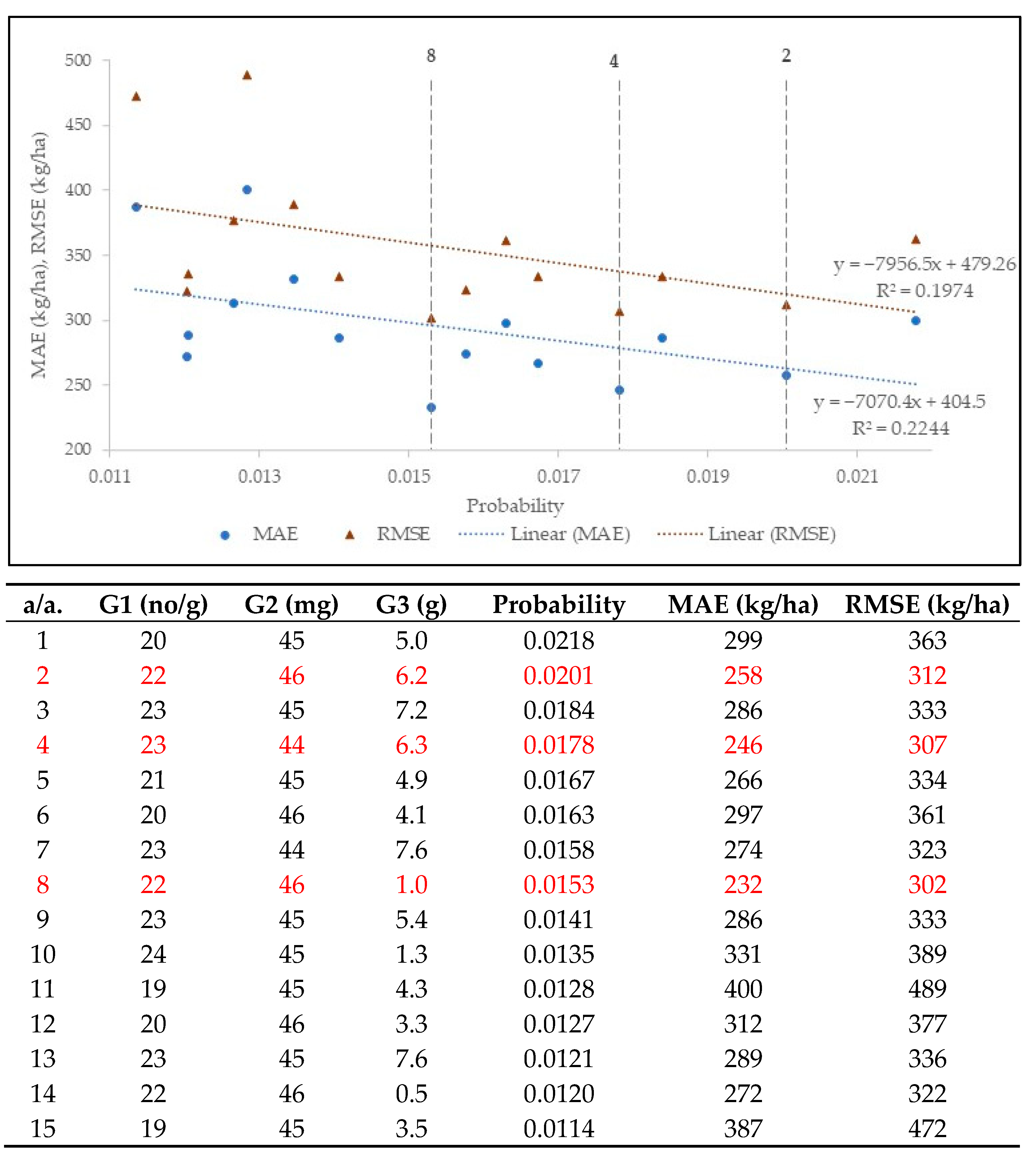
Notably, G1 and G2 exhibit lower variability, particularly at higher levels of probability, making them the most probable combinations. Figure 4 shows MAE and RMSE estimated between actual and simulated yield with the 15 sets of genetic parameters scoring the higher probabilities computed with GLUE. Regression analysis between MAE, RMSE, and probability showed that despite errors (i.e., MAE and RMSE) decreasing with increasing probability, (a) the slopes of the regression lines were not statistically significant at p = 0.05 (p-values of 0.07 for MAE and 0.10 for RMSE were found) and (b) weak association (as indicated by the low R2 values—0.22 and 0.20 for MAE and RMSE, respectively) between MAE and RMSE and probability was found. Such findings agree with these from James et al. (2013) [42], who also noted that changes in statistical measures, such as these used in this study, are likely not strongly associated with changes in probability. Besides the fact that the first combination is not necessarily the optimal one for the model, the accompanying Figure 4 table indicates that different sets of genetic parameters produce comparable values for statistical measures. Thus, the selection of the most appropriate genetic parameters can be determined by evaluating the statistical measures that are deemed most relevant for the intended application. These conclusions agree with a multi-model calibration study [4], which explored the advantages and disadvantages of several calibration methodologies but was unable to identify the most appropriate calibration procedures. They concluded that relying only on automatic calibration techniques may not be the best approach, although manual trial and error tends to produce non-optimal and non-replicable solutions.

3.3. Anthesis and Maturity fitting

The parameters of P1V and P1D for the three cultivars with the two calibration strategies (yield gap calibration (YgC) vs. calibration in rainfed mode (TrC)) were adjusted firstly, as suggested by the literature (e.g., [16,27]), using GLUE, to match the observed anthesis dates during 2004–2010. The selected values of P1V and P1D obtained by fitting the model to trial data are displayed in Table 2. The coefficients values between YgC and TrC are identical, suggesting that water and N stresses had no effect on simulated anthesis. Symeonidis (2011) [12] reported with DSSAT v3.5 similar values for P1V and significantly lower values (the ranking of cultivars was the same, however).
Although high correlation (R2 > 0.60) for anthesis dates was found from the comparison of all cultivars and calibration strategies, yield gap analysis produced a higher value for Mexicali, explaining about 8% more of the measured variability observed in the field (R2 was 0.699 vs. 0.621) and slightly worse values for Sifnos (R2 was 0.757 vs. 0.767, respectively) and Simeto (R2 was 0.776 vs. 0.803, respectively) (Figure 5). In contrast to MBE, lower MAE and RMSE were found by the YgC for Mexicali and Sifnos, regarding the former statistic, and Simeto, regarding for the latter. The yield gap analysis reproduced better (lower) statistical measures for this development stage for Sifnos than Mexicali and Simeto and the TrC for Simeto. The slopes and intercepts of the regression lines were in favor (closer to unity and zero, respectively) of the TrC for Mexicali and Simeto and of the YgC for Sifnos. The differences in statistical measures and regression characteristics between the two strategies is attributed to the different modes in which the crop model was run (potential mode for YgC vs. rainfed mode for TrC) and not to the yield gap analysis, which intends to improve yield predictions only.
The results achieved with DSSAT v3.5, for the same experiments (Table S2), are better compared with those found in this study (Figure 5). However, they were accomplished based on the assumptions related to initial soil water conditions mentioned in Section 2.2.4. With DSSAT v3.5, R2 between observed and simulated days to end ear growth was greater than 0.9, and the deviations between simulated and observed values for all cultivars ranged from 0.8 to 2.1 days for MAE, and from 1.1 to 3.4 days for RMSE, respectively.
The values of P5 for Mexicali, Sifnos, and Simeto were determined to be 555, 530, and 540 °C days, respectively, with YgC and 575, 560, and 570 °C days, respectively, with TrC. The respective values reported by Symeonidis (2011) [12] with DSSAT v3.5 were 490, 500, and 560 °C days (Table 2). Based on literature, these values are close to the range of 600–800 °C proposed by Kassie et al. (2016) [43] for durum wheat under Mediterranean climate conditions. Dettori et al. (2011) [17] and Rinaldi (2004) [27] reported 450 and 570 °C days, respectively, for Simeto in Italy. Rezzoug et al. (2008) [44] reported a substantially lower value of 322 °C days for Mexicali in Algeria.

3.4. Crop Yield Fitting

Table 2 also displays the values of G1, G2, and G3 coefficients for the three wheat cultivars obtained by fitting the crop model in the three different ways, as well as those from Symeonidis (2011) [12]. The values obtained with YgC_adj for the three cultivars compared to these from YgC_unadj were: similar for G2 (45–46 mg for the former strategy vs. 44–45 mg for the latter), slightly higher for G1 (21–23 no/g for YgC_adj vs. 17–18 no/g for YgC_unadj), and significantly lower for G3 (0.9–1.5 mg for YgC_adj vs. 5.6–7.3 mg for YgC_unadj). Apparently, since the final grain yield in CERES-Wheat is the product of plant population, kernels per plant (G1), and weight per kernel (G3) [45], the fitting process approximated observed yield by favoring kernel numbers for the YgC_adj strategy over kernel weight for the latter strategy. Compared to the rainfed strategies (TrC and DSSAT v3.5), the parameter values obtained with the YgC_adj strategy for the three cultivars were: significantly higher for G1 (21–23 no/g for the YgC_adj vs. 13–14 for the rainfed ones) and similar for G2 (in the range 45–46 mg for all three strategies). The values for G3 from the YgC_adj strategy were lower than these found with DSSAT v3.5 by Symeonidis (2011) [12] (0.9–1.5 mg for YgC_adj vs. 1.7–2.1 mg for DSSAT 3.5) and higher (except for Simeto) than the respective found with the TrC strategy.
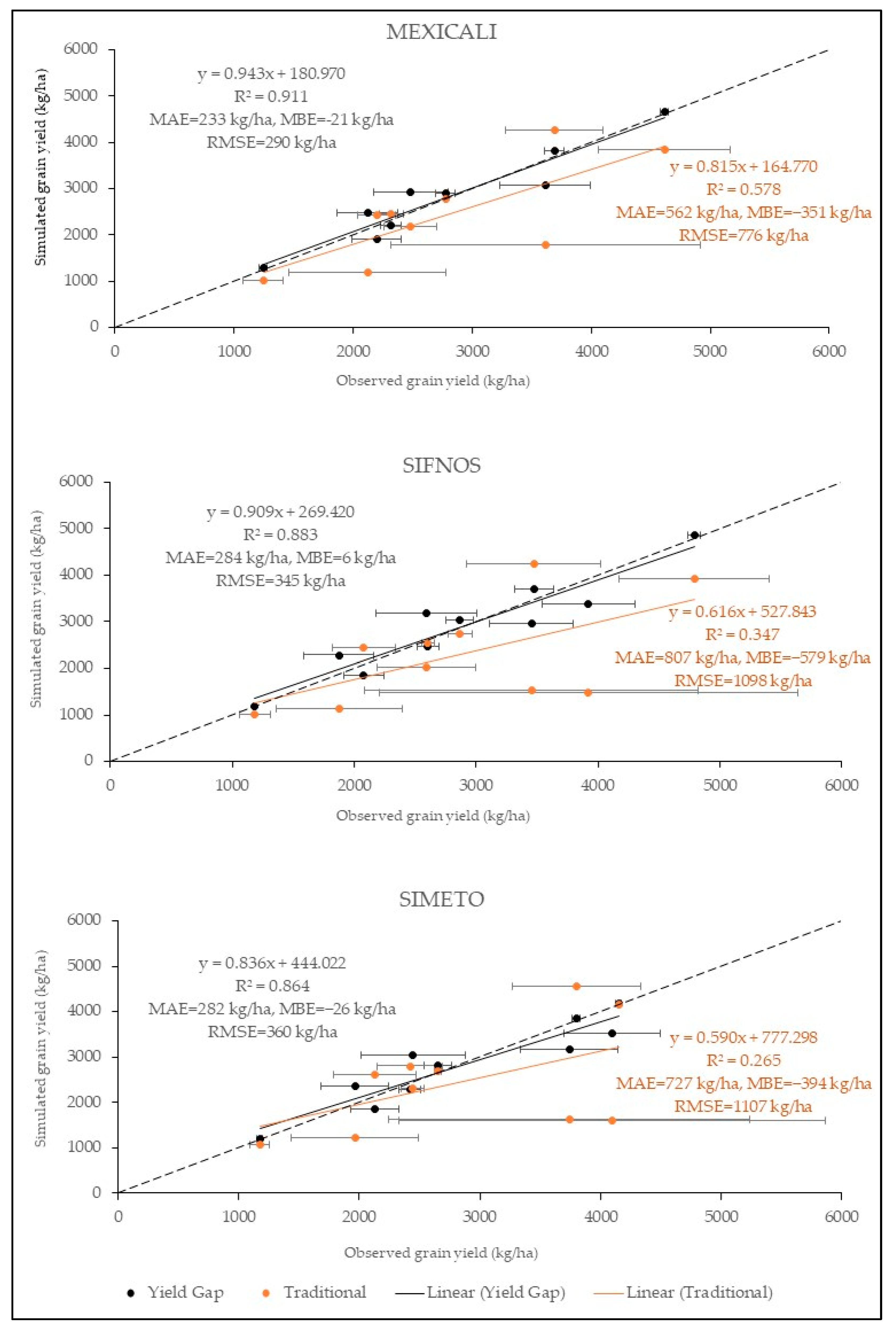
The yield gap-based calibration strategy accounting for year-to-year variability of Yrg (YgC_adj) was more effective than the “traditional” strategy (TrC) as most of the statistical measures were better. While very strong associations (R2 > 0.86) were found with the former strategy for the three cultivars between actual and simulated yields, only moderate (R2 was 0.347 for Sifnos and 0.265 for Simeto) and high (R2 was 0.578 for Mexicali) association was found from the latter strategy (Figure 6). MAE and RMSE were substantially lower with YgC_adj strategy than TrC for all cultivars and the slopes of the regression lines were closer to the 1:1 line.
As for the yield gap-based calibration strategy using an average site value of Yrg (YgC_unadj), the YgC_adj strategy was far more effective as all the statistical measures were much better (Figure S2). Only very weak (R2 ranged from 0 for Simeto to 0.056 for Mexicali) associations between measured and simulated yields were found with this strategy. The relative values of MAE and RMSE were significantly higher with the YgC_unadj strategy (36% and 48%, respectively, for Mexicali, 46% and 57%, respectively, for Sifnos and 42% and 53%, respectively, for Simeto) than YgC_adj, for all cultivars strategy (8% and 10%, respectively, for Mexicali, 10% and 12%, respectively, for Sifnos and 10% and 13%, respectively, for Simeto), and the slopes of the regression lines were almost parallel to the x axis.
The results from the YgC_adj strategy are compared to those with DSSAT v3.5 in Figure S3 and Table S2. Although very strong associations were found with both strategies, those with DSSAT v3.5 are closer to unity (R2 ranged 0.969 (Mexicali) to 0.984 (Sifnos) vs. 0.864 (Simeto) to 0.911 (Mexicali) with the YgC_adj). Except for the lower MBE with the YgC_adj strategy, relative MAE and RMSE were substantially lower with DSSAT v3.5 (6% and 8%, respectively, for Mexicali, 4% and 5%, respectively, for Sifnos, and 5% and 7%, respectively, for Simeto). The slopes of the regression lines were closer to the 1:1 line for Sifnos and Simeto with the latter method, while the slope for Mexicali was slightly closer with the former method.

3.5. Sensitivity Analysis

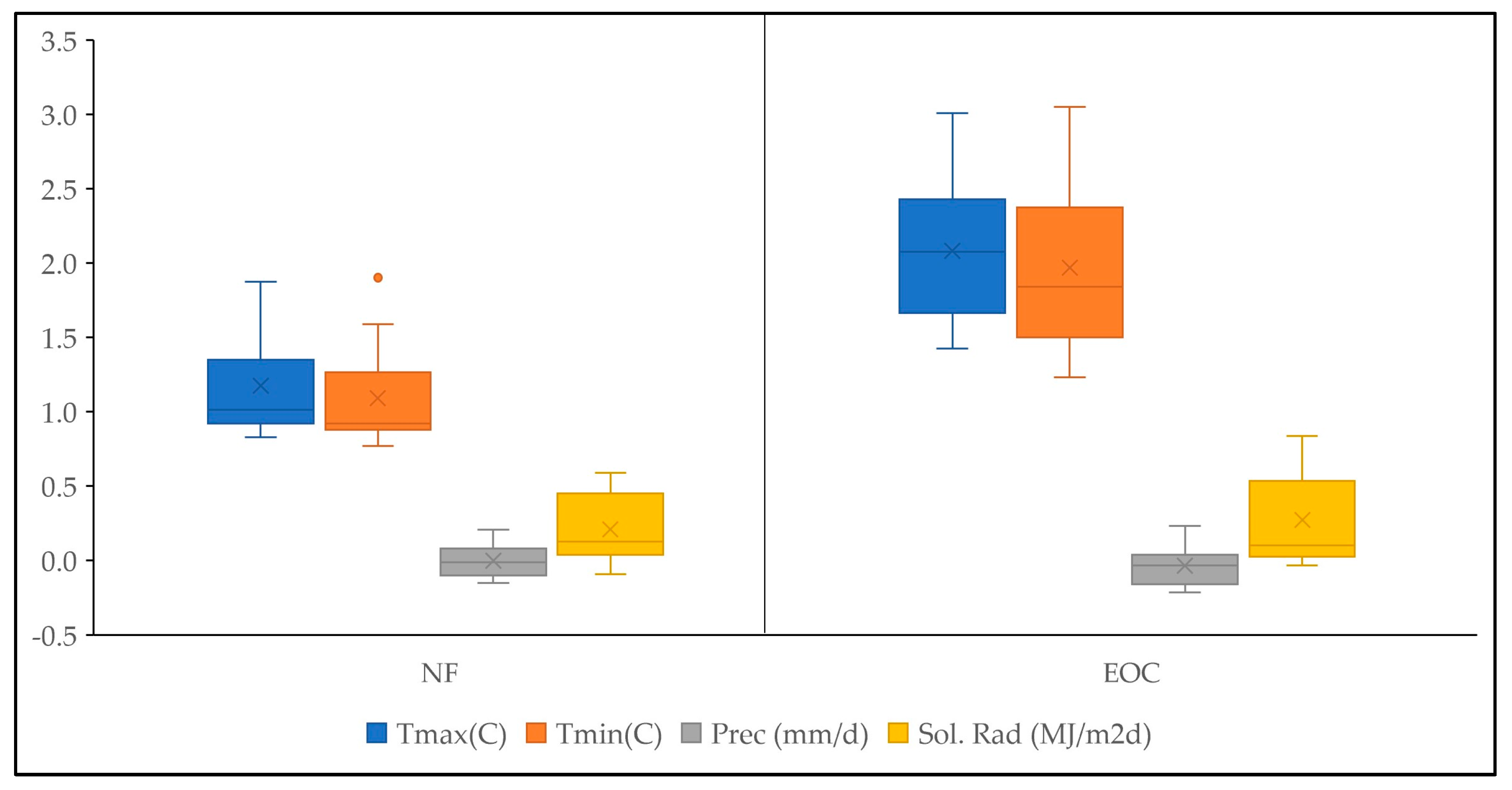
The anticipated differences in mean daily solar radiation, maximum (Tmax) and minimum (Tmin) air temperature, and precipitation from the EURO-CORDEX ensemble between the near-future (2021–2050) (NF) and the end-of-the-century (2071–2100) (EOC) with the reference period (1981–2005) (REF) for Thermi under the emission scenario RCP4.5 are shown in Figure 7. Average Tmax and Tmin temperatures in Thermi during the growing season (1 December–30 June) are expected to increase by approximately 1.2 °C and 1.1 °C, respectively, for the NF period and even higher (by approximately 2.1 °C and 2.0 °C, respectively) for EOC. Solar radiation will slightly increase (by about 1.3% and 1.7%) and precipitation will decrease (by almost 0.01 mm/day and 0.03 mm/day) for NF and EOC periods, respectively. Comparing these regional projections to those for Greece in general, under the RCP4.5 scenario, the average temperature during the growing season is expected to increase by 1.4 °C for NF and 2.3 °C for EOC. Precipitation is expected to decrease by 0.01 mm/day and 0.02 mm/day for the NF and EOC, respectively [39].
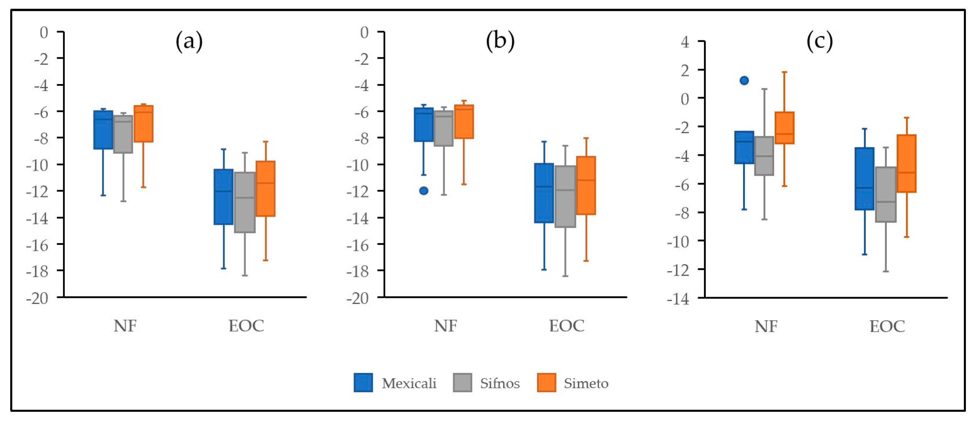
When the historical time series from the site’s meteorological station (covering the period 1979–2010) were independently adjusted (positive or negative) by the differences (11 such sensitivity experiments were conducted—one for each climate model) expected in NF and EOC (the genetic parameters produced with the YgC_adj strategy were used), crop simulated anthesis and maturity are anticipated to occur earlier, primarily due to increasing temperatures in Figure 7. Anthesis is showing a decrease by 8 days for the NF period and 13 days for EOC for Mexicali and Sifnos, and by 7 days for NF period and 12 days for EOC for Simeto (Figure 8a). As for maturity, decreases by 7 days for the NF period and 13 days for EOC for Mexicali, by 8 days for the NF period and 13 days for EOC for Sifnos, and by 8 days for NF period and 12 days for EOC for Simeto are projected (Figure 8b). On the other hand, the mean and median values of potential grain yield are expected to show a similar decrease for the three cultivars for each period, varying from 2.2 to 3.9% for the NF period, and from 5.0 to 7.1% for the EOC period (Figure 8c)
Similar reductions in anthesis, maturity, and yield for wheat cultivars have been observed, as well as in other Mediterranean regions for the period 2031–2060. For instance, according to [46], Sicily, Crete, and Cyprus have experienced a decrease in anthesis by 9 to 11 days and a decrease in maturity by 12 to 13 days. Moreover, there has been a reduction in grain yield values in these regions, with Cyprus and Crete showing a decrease of 2% and 7%, respectively, while Sicily has shown an increase of 6%.

4. Discussion

Results of numerous studies that rely on crop yield estimations (such as those related with climate change and food security), at global or regional spatial scales (e.g., [47,48]), have been compromised by uncertainties associated with poor crop model calibration and lack of transparency about underpinning assumptions (among others—see [5]) (e.g., [11]). In this context, there is an urgent need for an approach that will allow the determination of a genotype’s characteristics and minimize the numerous input-data required by crop models. This study proposes a methodology that facilitates the estimation of CERES-Wheat requirements by the genetic parameters for grain growth and yield based on the concept of yield gap, utilizing the GLUE coefficient estimator [6] and the global yield gap atlas (GYGA). The results of this methodology are compared with those of a traditional calibration strategy using data from yield trials, for three durum wheat cultivars, collected from the Aristotle University Farm in Thessaloniki, Greece, during 2004 to 2010.
Specifically, CERES-Wheat v4.7.5 was run in (a) potential mode with (ΥgC_adj strategy) and without (ΥgC_unadj strategy) accounting for the year-to-year variability of the relative yield gap Yrg and (b) rainfed mode, with water and nitrogen stresses simulated according to a common set of assumptions related to initial soil moisture (TrC strategy—[12]). Once the parameters affecting timing of anthesis and maturity in wheat (P1V, P1D, and P5) were adjusted to match observations, these affecting wheat yield potential (G1, G2, and G3) followed, utilizing the GLUE method. The proposed procedure is straightforward: the simulated potential yield for each year Yp is adjusted by the relative yield gap Yrg (the ratio between the yield gap Yg and the potential site yield Ysp) to achieve agreement with the actual yield Yac. Yg is calculated as the difference between Ysp and the actual yield Yac. The Yrg values (with (the ΥgC_adj strategy) and without (the ΥgC_unadj strategy) accounting for the year-to-year variability) were derived from the global yield gap atlas (GYGA) [32,33]. The WOFOST crop model [34] was used for their estimation [11]. Finally, the results of these strategies were compared with these obtained from Symeonidis (2011) [12] with DSSAT v.3.5 for the same set of yield trials. The primary findings are summarized as follows:
  • Regarding genetic coefficients: (i) the fitting process for all cultivars approximated the site yield by favoring grain numbers (G1) for the YgC_adj strategy over grain weight (G3) for the YgC_unadj strategy, while similar values for grain size (G2) were found for both strategies; and (ii) compared to the rainfed strategies (TrC and DSSAT 3.5), similar values for G2 and significantly higher values for G1 were obtained for all cultivars with the YgC_adj strategy. The values for G3 from the YgC_adj strategy were lower than these found with DSSAT v3.5 and higher (except for Simeto) than the respective obtained with the TrC strategy. Notably, the selection of the most appropriate genetic parameters in this study illustrated that statistical measures (such as MAE and RMSE) more relevant for the intended application could be preferred over the probability estimated by GLUE since different sets of genetic parameters produce similar statistical measure estimates.
  • The yield gap-based calibration strategy accounting for year-to-year variability of Yrg (YgC_adj) was: (i) superior to the “traditional” strategy (TrC) for all cultivars, as MAE and RMSE were substantially lower with the former strategy and the slopes of the regression lines were closer to the 1:1 line; (ii) more effective than the respective calibration strategy using an average site value of Yrg (YgC_unadj) showing much lower relative MAE (from 36 to 46% for YgC_unadj vs. 8 to 10% for YgC_adj) and RMSE (from 48 to 57% for YgC_unadj vs. 10 to 13% for YgC_adj) values. These results confirm the importance of incorporating temporal variability into yield gap analysis conducted at the farming systems level, as noted by Silva and Ramisch (2018) [49]; and (iii) slightly inferior to calibration with DSSAT v.3.5, which presented closer to 1:1 regression lines and lower relative MAE and RMSE values (6% and 8%, respectively, for Mexicali, 4% and 5%, respectively, for Sifnos, and 5% and 7%, respectively, for Simeto). The different results show the sensitivity of the two crop model versions to the initial soil moisture conditions assumed by Symeonidis (2011) [12]. The substantial impacts of uncertainties in soil and management information on crop simulated water, N, and yield were confirmed in recent studies [50,51].
  • The sensitivity analysis of simulated wheat development and yield, applying the genetic parameters produced with the YgC_adj strategy, based on climate change projections from the ensemble of 11 high-resolution EURO-CORDEX regional climate model simulations, under the influence of the moderate mitigation emission scenario RCP4.5 for the future periods 2021–2050 (NF) and 2071–2100 (EOC), revealed: alike earlier anthesis and maturity (by 7–8 and 12–13 days, on average, for the NF and the EOC, respectively) and decreased yield (from 2.2 to 3.9% for the NF period, and from 5.0 to 7.1% for the EOC) as a result of the increased temperature and solar radiation (by 1.4 °C and 1.3%, for the NF, and 2.3 °C and 1.7%, for the end EOC, respectively).

5. Conclusions

The proposed methodology provides a transparent, reproducible, and scientifically robust guideline for crop model calibration since on potential mode (i) it requires no more knowledge of site-specific initial soil moisture (not routinely measured) and other management practices (such as fertilizer application information); therefore, it substantially minimizes data input requirements and (ii) the performance of CERES-Wheat, and generally of crop models, is more satisfactory than under resource-limiting conditions in some growing stages [52,53]. Further testing of this methodology with different plants, crop models, and environmental conditions is required.
Furthermore, reliable and accurate assessment of yield gaps at the farming systems level is challenging, even without considering the effects of future climate change [49,54]. There are several methods for estimating yield gaps, including field experiments, yield contests, maximum farmer yields based on surveys, and crop model simulations [11,55]. Field experiments involve controlled trials of different crops or cultivation techniques, while yield contests encourage farmers to compete to achieve the highest yields. Maximum farmer yields based on surveys involve surveying farmers to determine their highest yields in the past [56,57]. Crop simulation models provide the most robust approach because they account for the interactive effects of genotype, weather, and management (GxExM) on yields across agroecological zones and years [11]. Finally, the choice of the spatial framework (for the differences between top-bottom vs. bottom-up approaches, see Figure 1 in Edreira et al. (2021) [29]) for robust estimation of yield potential and gaps for assessing future food security constitutes an additional challenge on the use of crop models, since the abovementioned study revealed large discrepancies across all spatial levels.

Supplementary Materials

The following supporting information can be downloaded at: https://www.mdpi.com/article/10.3390/land12071372/s1, Figure S1: Actual Yield (Ya) (kg dm/ha), Yield Gap (Yp-Ya) (kg dm/ha), relative Yield Gap (1-Yrg) and average rela-tive Yield Gap for Sifnos and Simeto. Planting dates of the reported years are also shown on the horizontal axis; Figure S2: Comparison of the two calibration strategies (“Traditional (TrC)” vs “Yield gap (YgC_unadj)”) grain yield for the three cultivars (Mexicali (n = 9), Sifnos (n = 10) and Simeto (n = 10)); Figure S3: Comparison of the two calibration strategies (“DSSAT 3.5” vs “Yield gap (YgC_unadj)”) grain yield for the three cultivars (Mexicali (n = 9), Sifnos (n = 10) and Simeto (n = 10)); Table S1: The EURO-CORDEX regional climate models whose simulations were used in the present study; Table S2: Statistical indicators (correlation coefficient r, mean absolute error (MAE), mean bias (MBE), root mean squared error (RMSE) and the slope of the regression line (slope)) of the evaluation of CERES-Wheat results for an-thesis and yield for the three cultivars with DSSAT 3.5 (Symeonidis, 2011).

Author Contributions

Conceptualization, T.M.; methodology, T.M.; software, M.N.; validation, M.N. and T.M.; formal analysis, M.N.; investigation, M.N. and T.M.; data curation, M.N.; writing—original draft preparation, M.N.; writing—review and editing, M.N. and T.M; visualization, M.N.; project administration, T.M. All authors have read and agreed to the published version of the manuscript.

Funding

This research received funding from the action titled “National Network on Climate Change and its Impacts—CLIMPACT” (grant no. 2018SE01300001), which is implemented under sub-project 3 of the project “Infrastructure of national research networks in the fields of Precision Medicine, Quantum Technology and Climate Change”, funded by the Public Investment Program of Greece, General Secretary of Research, and Technology/Ministry of Development and Investments.

Data Availability Statement

The EURO-CORDEX simulations used for the analysis are publicly available via https://esgf-data.dkrz.de/search/cordex-dkrz/, accessed on 7 June 2023.

Acknowledgments

We thank A.K. Georgoulias, D. Akritidis, and P. Zanis for providing the EURO-CORDEX data for this work. We acknowledge the World Climate Research Program’s Working Group on Regional Climate, and the Working Group on Coupled Modelling, the former coordinating body of CORDEX and the panel responsible for CMIP5. We also acknowledge the Earth System Grid Federation infrastructure, an international effort led by the U.S. Department of Energy’s Program for Climate Model Diagnosis and Intercomparison, the European Network for Earth System Modelling, and other partners in the Global Organization for Earth System Science Portals (GO-ESSP).

Conflicts of Interest

The authors declare no conflict of interest.

References

  1. Schulze, R.; Durand, W. Maize Production in South Africa and Climate Change. In Handbook for Farmers, Officials and Other Stakeholders on Adaptation to Climate Change in the Agriculture Sector within South Africa; Schulze, R.E., Ed.; Section C: Crops in South Africa and Climate Change, South Africa, 2016. [Google Scholar]
  2. Asseng, S.; Zhu, Y.; Basso, B.; Wilson, T.; Cammarano, D. Simulation Modeling: Applications in Cropping Systems. Encycl. Agric. Food Syst. 2014, 5, 102–112. [Google Scholar] [CrossRef]
  3. Kephe, P.N.; Ayisi, K.K.; Petja, B.M. Challenges and opportunities in crop simulation modelling under seasonal and projected climate change scenarios for crop production in South Africa. Agric. Food Secur. 2021, 10, 10. [Google Scholar] [CrossRef]
  4. Wallach, D.; Palosuo, T.; Thorburn, P.; Hochman, Z.; Gourdain, E.; Andrianasolo, F.; Asseng, S.; Basso, B.; Buis, S.; Crout, N.; et al. The chaos in calibrating crop models: Lessons learned from a multi-model calibration exercise. Environ. Model. Softw. 2021, 145, 105206. [Google Scholar] [CrossRef]
  5. Grassini, P.; van Bussel, L.G.J.; Van Wart, J.; Wolf, J.; Claessens, L.; Yang, H.; Boogaard, H.; de Groot, H.; van Ittersum, M.K.; Cassman, K.G. How good is good enough? Data requirements for reliable crop yield simulations and yield-gap analysis. Field Crop. Res. 2015, 177, 49–63. [Google Scholar] [CrossRef] [Green Version]
  6. Jones, J.W.; He, J.; Boote, K.J.; Wilkens, P.; Porter, C.H.; Hu, Z. Estimating DSSAT Cropping System Cultivar-Specific Parameters Using Bayesian Techniques. Methods Introd. Syst. Model. into Agric. Res. 2011, 2, 365–393. [Google Scholar] [CrossRef]
  7. Seidel, S.J.; Palosuo, T.; Thorburn, P.; Wallach, D. Towards improved calibration of crop models—Where are we now and where should we go? Eur. J. Agron. 2018, 94, 25–35. [Google Scholar] [CrossRef]
  8. Annicchiarico, P. Genotype x Environment Interaction: Challenges and Opportunities for Plant Breeding and Cultivar Recommendations; FAO: Rome, Italy, 2002. [Google Scholar]
  9. Choruma, D.; Balkovic, J.; Odume, O.N. Calibration and validation of the EPIC model for maize production in the Eastern Cape, South Africa. Agronomy 2019, 9, 494. [Google Scholar] [CrossRef] [Green Version]
  10. Jones, J.W.; Antle, J.M.; Basso, B.; Boote, K.J.; Conant, R.T.; Foster, I.; Godfray, H.C.J.; Herrero, M.; Howitt, R.E.; Janssen, S.; et al. Toward a new generation of agricultural system data, models, and knowledge products: State of agricultural systems science. Agric. Syst. 2017, 155, 269–288. [Google Scholar] [CrossRef]
  11. Van Ittersum, M.K.; Cassman, K.G.; Grassini, P.; Wolf, J.; Tittonell, P.; Hochman, Z. Yield gap analysis with local to global relevance-A review. Field Crop. Res. 2013, 143, 4–17. [Google Scholar] [CrossRef] [Green Version]
  12. Symeonidis, K.; Mavromatis, T.; Kotzamanidis, S. Investigating with the Ceres-Wheat Model the Impacts of Soil and Climate Factors on Durum Wheat Performance and Earliness in Northern Greece. Springer Atmospheric Sciences; Springer: Berlin/Heidelberg, Germany, 2013. [Google Scholar] [CrossRef]
  13. Jones, C.A.; Kiniry, J.R.; Dyke, P.T. CERES-Maize: A Simulation Model of Maize Growth and Development; A&M Univ. Press: College Station, TX, USA, 1986. [Google Scholar]
  14. Suleiman, A.A.; Ritchie, J.T. Estimating Saturated Hydraulic Conductivity from Soil Porosity. Trans. ASAE 2001, 44, 235. [Google Scholar] [CrossRef]
  15. Hoogenboom, G.; Porter, C.H.; Boote, K.J.; Shelia, V.; Wilkens, P.W.; Singh, U.; White, J.W.; Asseng, S.; Lizaso, J.I.; Moreno, L.P.; et al. The DSSAT Crop Modeling Ecosystem, In Advances in Crop Modelling for a Sustainable Agriculture; Burleigh Dodds Science Publishing: Cambridge, UK, 2019; pp. 173–216. [Google Scholar]
  16. Jones, J.W.; Hoogenboom, G.; Porter, C.H.; Boote, K.J.; Batchelor, W.D.; Hunt, L.A.; Wilkens, P.W.; Singh, U.; Gijsman, A.J.; Ritchie, J.T. The DSSAT cropping system model. Eur. J. Agron. 2003, 18, 235–265. [Google Scholar] [CrossRef]
  17. Dettori, M.; Cesaraccio, C.; Motroni, A.; Spano, D.; Duce, P. Using CERES-Wheat to simulate durum wheat production and phenology in Southern Sardinia, Italy. Field Crop. Res. 2011, 120, 179–188. [Google Scholar] [CrossRef]
  18. Dettori, M.; Cesaraccio, C.; Duce, P. Simulation of climate change impacts on production and phenology of durum wheat in Mediterranean environments using CERES-Wheat model. Field Crop. Res. 2017, 206, 43–53. [Google Scholar] [CrossRef]
  19. Eitzinger, J.; Trnka, M.; Hösch, J.; Žalud, Z.; Dubrovský, M. Comparison of CERES, WOFOST and SWAP models in simulating soil water content during growing season under different soil conditions. Ecol. Modell. 2004, 171, 223–246. [Google Scholar] [CrossRef]
  20. Beven, K.; Binley, A. The future of distributed models: Model calibration and uncertainty prediction. Hydrol. Process. 1992, 6, 279–298. [Google Scholar] [CrossRef]
  21. Franks, S.W.; Gineste, P.; Beven, K.J.; Mérot, P. On constraining the predictions of a distributed model: The incorporation of fuzzy estimates of saturated areas into the calibration process. Water Resour. Res. 1998, 34, 787–797. [Google Scholar] [CrossRef]
  22. Schulz, K.; Beven, K.; Huwe, B. Equifinality and the Problem of Robust Calibration in Nitrogen Budget Simulations. Soil Sci. Soc. Am. J. 1999, 63, 1934–1941. [Google Scholar] [CrossRef]
  23. Romanowicz, R.J.; Beven, K.J. Comments on generalised likelihood uncertainty estimation. Reliab. Eng. Syst. Saf. 2006, 91, 1315–1321. [Google Scholar] [CrossRef]
  24. Niu, J.Y.; Gan, Y.T.; Zhang, J.W.; Yang, Q.F. Postanthesis dry matter accumulation and redistribution in spring wheat mulched with plastic film. Crop. Sci. 1998, 38, 1562–1568. [Google Scholar] [CrossRef]
  25. Zhang, D.; Wang, H.; Li, D.; Li, H.; Ju, H.; Li, R.; Batchelor, W.D.; Li, Y. DSSAT-CERES-Wheat model to optimize plant density and nitrogen best management practices. Nutr. Cycl. Agroecosyst. 2019, 114, 19–32. [Google Scholar] [CrossRef]
  26. Mereu, V.; Gallo, A.; Spano, D. Optimizing genetic parameters of CSM-CERES wheat and CSM-CERES maize for durum wheat, common wheat, and maize in Italy. Agronomy 2019, 9, 665. [Google Scholar] [CrossRef] [Green Version]
  27. Rinaldi, M. Water availability at sowing and nitrogen management of durum wheat: A seasonal analysis with the CERES-Wheat model. Field Crop. Res. 2004, 89, 27–37. [Google Scholar] [CrossRef]
  28. Ji, J.; Cai, H.; He, J.; Wang, H. Performance evaluation of CERES-Wheat model in Guanzhong Plain of Northwest China. Agric. Water Manag. 2014, 144, 1–10. [Google Scholar] [CrossRef]
  29. Rattalino Edreira, J.I.; Andrade, J.F.; Cassman, K.G.; van Ittersum, M.K.; van Loon, M.P.; Grassini, P. Spatial frameworks for robust estimation of yield gaps. Nat. Food 2021, 2, 773–779. [Google Scholar] [CrossRef]
  30. van Bussel, L.G.J.; Grassini, P.; Van Wart, J.; Wolf, J.; Claessens, L.; Yang, H.; Boogaard, H.; de Groot, H.; Saito, K.; Cassman, K.G.; et al. From field to atlas: Upscaling of location-specific yield gap estimates. Field Crop. Res. 2015, 177, 98–108. [Google Scholar] [CrossRef] [Green Version]
  31. Habte, A.; Worku, W.; Gayler, S.; Ayalew, D.; Mamo, G. Model-based yield gap analysis and constraints of rainfed sorghum production in Southwest Ethiopia. J. Agric. Sci. 2020, 158, 855–869. [Google Scholar] [CrossRef]
  32. Global Yield Gap Atlas. Available online: https://www.yieldgap.org/ (accessed on 7 June 2023).
  33. Grassini, P.; Cassman, K.G.; van Ittersum, M.K. Exploring Maize Intensification with the Global Yield Gap Atlas. Better Crop. Plant Food 2017, 101, 7–9. [Google Scholar]
  34. De Wit, A.; Boogaard, H.; Fumagalli, D.; Janssen, S.; Knapen, R.; van Kraalingen, D.; Supit, I.; van der Wijngaart, R.; van Diepen, K. 25 years of the WOFOST cropping systems model. Agric. Syst. 2019, 168, 154–167. [Google Scholar] [CrossRef]
  35. Pirttioja, N.; Palosuo, T.; Fronzek, S.; Räisänen, J.; Rötter, R.P.; Carter, T.R. Using impact response surfaces to analyse the likelihood of impacts on crop yield under probabilistic climate change. Agric. For. Meteorol. 2019, 264, 213–224. [Google Scholar] [CrossRef]
  36. Ceglar, A.; van der Wijngaart, R.; de Wit, A.; Lecerf, R.; Boogaard, H.; Seguini, L.; van den Berg, M.; Toreti, A.; Zampieri, M.; Fumagalli, D.; et al. Improving WOFOST model to simulate winter wheat phenology in Europe: Evaluation and effects on yield. Agric. Syst. 2019, 168, 168–180. [Google Scholar] [CrossRef]
  37. Jacob, D.; Petersen, J.; Eggert, B.; Alias, A.; Christensen, O.B.; Bouwer, L.M.; Braun, A.; Colette, A.; Déqué, M.; Georgievski, G.; et al. EURO-CORDEX: New high-resolution climate change projections for European impact research. Atmosphere 2014, 14, 563–578. [Google Scholar] [CrossRef]
  38. Vautard, R.; Gobiet, A.; Jacob, D.; Belda, M.; Colette, A.; Déqué, M.; Fernández, J.; García-Díez, M.; Goergen, K.; Güttler, I.; et al. The simulation of European heat waves from an ensemble of regional climate models within the EURO-CORDEX project. Clim. Dyn. 2013, 41, 2555–2575. [Google Scholar] [CrossRef]
  39. Georgoulias, A.K.; Akritidis, D.; Kalisoras, A.; Kapsomenakis, J.; Melas, D.; Zerefos, C.S.; Zanis, P. Climate change projections for Greece in the 21st century from high-resolution EURO-CORDEX RCM simulations. Atmos. Res. 2022, 271, 106049. [Google Scholar] [CrossRef]
  40. Hinkle, D.E.; Wiersma, W.; Jurs, S. Applied Statistics for the Behavioral Sciences, 5th ed.; Houghton Mifflin: Boston, MA, USA, 2003. [Google Scholar]
  41. Bao, Y.; Hoogenboom, G.; McClendon, R.; Vellidis, G. A comparison of the performance of the CSM-CERES-Maize and EPIC models using maize variety trial data. Agric. Syst. 2017, 150, 109–119. [Google Scholar] [CrossRef] [Green Version]
  42. James, G.; Witten, D.; Hastie, T.; Tibshirani, R. An Introduction to Statistical Learning wth Application in R; Springer: New York, NY, USA, 2013; ISBN 9781461471370. [Google Scholar]
  43. Kassie, B.T.; Asseng, S.; Porter, C.H.; Royce, F.S. Performance of DSSAT-Nwheat across a wide range of current and future growing conditions. Eur. J. Agron. 2016, 81, 27–36. [Google Scholar] [CrossRef] [Green Version]
  44. Rezzoug, W.; Gabrielle, B.; Suleiman, A.; Benabdeli, K. Application and evaluation of the DSSAT-wheat in the Tiaret region of Algeria. J. Agric. Res. 2008, 3, 284–296. [Google Scholar]
  45. Ritchie, J.T.; Otter, S. Description and performance of CERES-Wheat: A user-oriented wheat yield model. Usda-Ars 1985, 38, 159–175. [Google Scholar]
  46. Life ADAPT2CLIMA. Adaptation to Climate Change Impacts on the Mediterranean islands’ Agriculture. 2017. Available online: http://adapt2clima.eu/uploads/2017/adapt2clima_Deliverable_C.4.2_final.pdf (accessed on 7 June 2023).
  47. Challinor, A.J.; Watson, J.; Lobell, D.B.; Howden, S.M.; Smith, D.R.; Chhetri, N. A meta-analysis of crop yield under climate change and adaptation. Nat. Clim. Chang. 2014, 4, 287–291. [Google Scholar] [CrossRef] [Green Version]
  48. Rosenzweig, C.; Elliott, J.; Deryng, D.; Ruane, A.C.; Müller, C.; Arneth, A.; Boote, K.J.; Folberth, C.; Glotter, M.; Khabarov, N.; et al. Assessing agricultural risks of climate change in the 21st century in a global gridded crop model intercomparison. Proc. Natl. Acad. Sci. USA 2014, 111, 3268–3273. [Google Scholar] [CrossRef]
  49. Silva, J.V.; Ramisch, J.J. Whose gap counts? the role of yield gap analysis within a development-oriented agronomy. Exp. Agric. 2018, 55, 311–338. [Google Scholar] [CrossRef] [Green Version]
  50. Archontoulis, S.V.; Castellano, M.J.; Licht, M.A.; Nichols, V.; Baum, M.; Huber, I.; Martinez-Feria, R.; Puntel, L.; Ordóñez, R.A.; Iqbal, J.; et al. Predicting crop yields and soil-plant nitrogen dynamics in the US Corn Belt. Crop. Sci. 2020, 60, 721–738. [Google Scholar] [CrossRef] [Green Version]
  51. Basso, B.; Hyndman, D.W.; Kendall, A.D.; Grace, P.R.; Robertson, G.P. Can impacts of climate change and agricultural adaptation strategies be accurately quantified if crop models are annually re-initialized? PLoS ONE 2015, 10, 0127333. [Google Scholar] [CrossRef] [Green Version]
  52. Timsina, J.; Humphreys, E. Performance of CERES-Rice and CERES-Wheat models in rice-wheat systems: A review. Agric. Syst. 2006, 90, 5–31. [Google Scholar] [CrossRef]
  53. Wei, Y.; Ru, H.; Leng, X.; He, Z.; Ayantobo, O.O.; Javed, T.; Yao, N. Better Performance of the Modified CERES-Wheat Model in Simulating Evapotranspiration and Wheat Growth under Water Stress Conditions. Agriculture 2022, 12, 1902. [Google Scholar] [CrossRef]
  54. Ollenburger, M.; Kyle, P.; Zhang, X. Uncertainties in estimating global potential yields and their impacts for long-term modeling. Food Secur. 2022, 14, 1177–1190. [Google Scholar] [CrossRef]
  55. Lobell, D.B.; Cassman, K.G.; Field, C.B. Crop yield gaps: Their importance, magnitudes, and causes. Annu. Rev. Environ. Resour. 2009, 34, 179–204. [Google Scholar] [CrossRef] [Green Version]
  56. Grassini, P.; Thorburn, J.; Burr, C.; Cassman, K.G. High-yield irrigated maize in the Western U.S. Corn Belt: I. On-farm yield, yield potential, and impact of agronomic practices. Field Crop. Res. 2011, 120, 142–150. [Google Scholar] [CrossRef] [Green Version]
  57. Laborte, A.G.; de Bie, K.C.A.J.M.; Smaling, E.M.A.; Moya, P.F.; Boling, A.A.; Van Ittersum, M.K. Rice yields and yield gaps in Southeast Asia: Past trends and future outlook. Eur. J. Agron. 2012, 36, 9–20. [Google Scholar] [CrossRef]
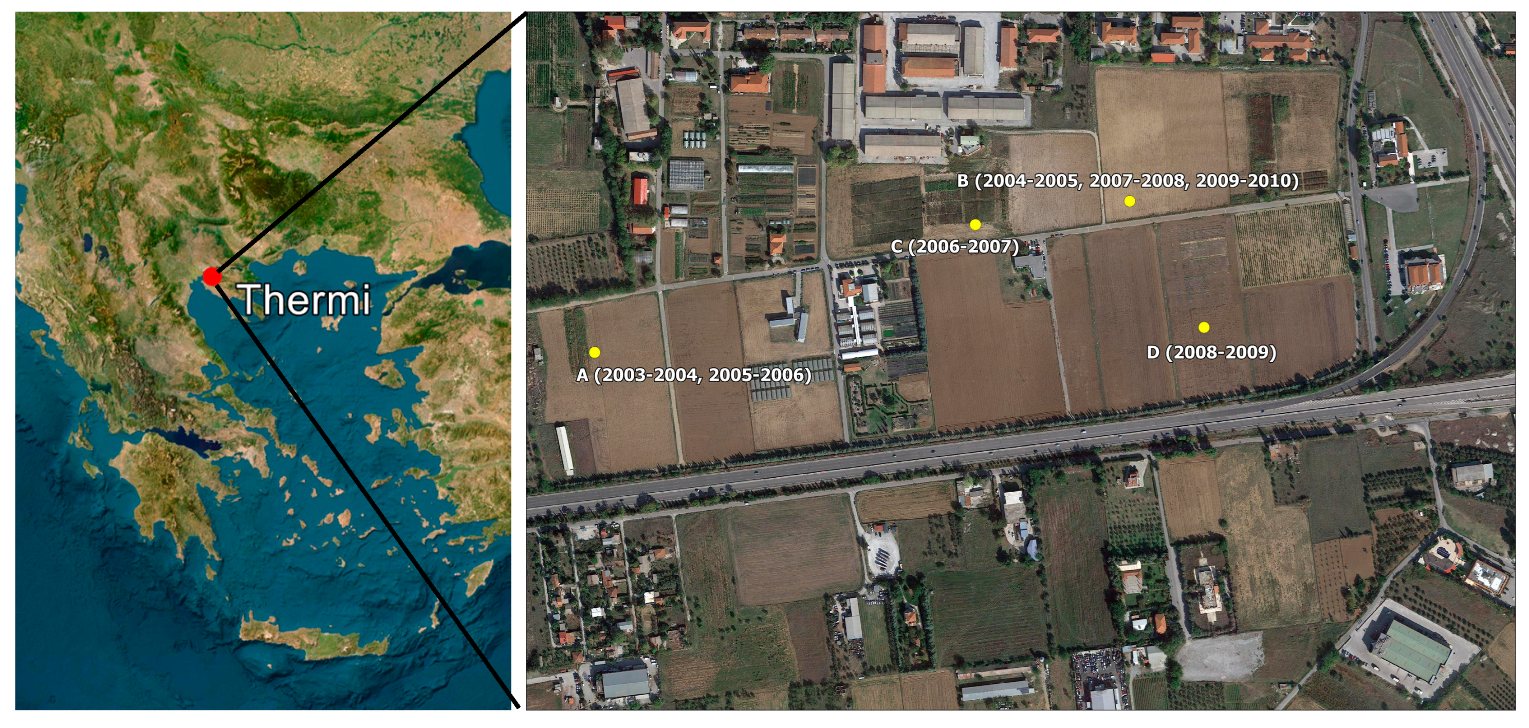
Figure 1. The study area (red dot) and site-years of experiments (yellow dots).
Land 12 01372 g001
Figure 2. Actual yield (Ya) (kg/ha), yield gap (Yp-Ya) (kg/ha), relative yield gap (1-Yrg), and average relative yield gap for Mexicali. Planting dates of the reported years are also shown on the horizontal axis.
Land 12 01372 g002
Figure 3. Mexicali’s 100 most probable combinations of genetic parameters of G1 (no/g), G2 (mg), and G3 (g) and their corresponding probabilities.
Land 12 01372 g003
Figure 4. MAE and RMSE of the first 15 most probable combinations of Mexicali’s G1, G2, and G3 coefficients (plot) identified by GLUE. The combinations with lower MAE and RMSE are noted in the figure and shown (in red fonts) in the table.
Land 12 01372 g004
Figure 5. Comparison of the two calibration strategies (“Traditional (TrC)” vs. “Yield gap (YgC_adj)”) anthesis dates for the three cultivars (Mexicali (n = 9), Sifnos (n = 10) and Simeto (n = 10)). Bars indicate standard deviations of observations in relation to the average. The solid lines represent the linear regression fits to crop data, while the dotted line represents the 1:1 line.
Land 12 01372 g005
Figure 6. Comparison of the two calibration strategies (“Traditional (TrC)” vs. “Yield gap (YgC_adj)”) grain yield for the three cultivars (Mexicali (n = 9), Sifnos (n = 10), and Simeto (n = 10)). Bars indicate standard deviations of observations in relation to the average. The solid lines represent the linear regression fits to crop data, while the dotted line represents the 1:1 line.
Land 12 01372 g006
Figure 7. Differences in maximum (Tmax) and minimum (Tmin) air temperature, daily solar radiation (Sol. Rad.), and precipitation (Prec.) during the growing season (1 December–30 June) from the EURO-CORDEX ensemble between the near-future (2021–2050) (NF-left part) and the end-of-the-century (2071–2100) (EOC-right part) and the reference period (1981–2005) (REF) for Thermi (northern Greece) for the emission scenario RCP4.5.
Land 12 01372 g007
Figure 8. Differences in simulated with CERES-Wheat (a) anthesis (Julian Date), (b) maturity (Julian Date), and (c) grain yield (%) for the near future (2021–2050) and the end of century (2071–2100) periods.
Land 12 01372 g008
Table 1. Genetic parameters of wheat cultivars for CERES-Wheat.
ParameterDefinitionUnit
P1VDays at the optimum vernalizing temperature required to complete vernalizationdays
P1DPercentage reduction in development rate in a photoperiod 10 h shorter than the threshold relative to that at the threshold
P5Grain filling (excluding lag) phase duration°C day
PHINTInterval between successive leaf tip appearances°C day
G1Kernel number per unit canopy weight at anthesisnο/g
G2Standard kernel size under optimum conditionsmg
G3Standard non-stressed dry weight (including grain) of a single tiller at maturityg
Table 2. Genetic parameters of wheat cultivars from fitting CERES-Wheat (DSSAT v. 4.7.5 (with the two calibration strategies (in potential model with and without interannual relative yield gap variability (Yrg) considered, and in rainfed mode (TrC)) and DSSAT v. 3.5 [12]).
DSSAT v4.7.5 (YgC with Year Adjustment of Yrg (ΥgC_adj))
Cultivars1 P1V1 P1D1 P51 G11 G21 G31 PHINT
Mexicali545155522461.598
Sifnos475253023450.999
Simeto585954021450.998
DSSAT v4.7.5 (YgC without Year Adjustment of Yrg (YgC_unadj))
CultivarsP1VP1DP5G1G2G3PHINT
Mexicali545155518457.3100
Sifnos475253017456.9100
Simeto585954017445.699
DSSAT v4.7.5 (TrC—Rainfed Mode)
CultivarsP1VP1DP5G1G2G3PHINT
Mexicali545157513450.6100
Sifnos475256013460.798
Simeto585957014466.9100
DSSAT v3.5
CultivarsP1VP1DP5G1G2G3PHINT
Mexicali523249014581.791
Sifnos553450014582.193
Simeto623756014562.190
1: See Table 1 for parameter definitions.
Disclaimer/Publisher’s Note: The statements, opinions and data contained in all publications are solely those of the individual author(s) and contributor(s) and not of MDPI and/or the editor(s). MDPI and/or the editor(s) disclaim responsibility for any injury to people or property resulting from any ideas, methods, instructions or products referred to in the content.