Article

Evaluation of Biodiversity Maintenance Capacity in Forest Landscapes: A Case Study in Beijing, China

1
School of Landscape Architecture, Beijing Forestry University, Beijing 100083, China
2
Beijing Laboratory for Urban and Rural Ecological Environment, Beijing 100083, China
3
Research Institute for Beautiful China’s Human Settlements and Ecological Environment, Beijing 100083, China
*
Author to whom correspondence should be addressed.
Land 2023, 12(7), 1293; https://doi.org/10.3390/land12071293
Submission received: 1 June 2023 / Revised: 20 June 2023 / Accepted: 25 June 2023 / Published: 26 June 2023
(This article belongs to the Section Landscape Ecology)

Abstract

:
Understanding how landscape pattern changes impact forest biodiversity conservation and ecosystem management is crucial. This study evaluated the biodiversity maintenance capacity (BMC) of forest landscapes in Beijing, China from 2005 to 2020 based on habitat quality and carbon sink. For this, the moving window method was employed to compute landscape indices that depict variations in landscape patterns, including intermixing, connectivity, diversity, and compactness. Lastly, the relationship between landscape pattern changes and the BMC of forest landscapes was investigated using a combination of spatial correlation analysis and geographic weighted regression measurement models. The results showed the following. (1) The average BMC increased from 0.798 to 0.822. Spatially, 84.14% of the areas experienced an improvement, mainly in the mountainous region. In contrast, a decrease was observed in 4.03% of the areas, primarily concentrated in the transition zone between mountains and suburban plain. (2) The landscape pattern changed dramatically from 2005 to 2020. Landscape intermixing and compactness decreased slightly by 11.45% and 7.82%, while landscape connectivity and diversity increased significantly by 64.28% and 55.44%, respectively. (3) The BMC’s global Moran’s I values in 2005 and 2020 were 0.711 and 0.782, respectively, signifying a spatial bipolar agglomeration pattern. (4) Among the four selected landscape indices, the compactness was found to be the most critical factor. It attained a positive contribution to forests with high BMC, but had a negative impact on forests with low BMC. The results could provide a reference for planners coordinating forest management and biodiversity conservation.

1. Introduction

The alteration of landscape patterns resulting from urbanization is widely acknowledged as a significant contributor to the global decline in biodiversity and biotic homogenization [1]. At the same time, cities also face increasing climatic pressures and threats to the survival of many species and types of natural communities [2,3]. Currently, over 50% of the global population resides in urban areas. By 2030, the global urbanized land area is projected to double, with the majority of future urban expansion taking place in global biodiversity hotspots such as China [4]. Urban expansion leads to a continued decline in urban biodiversity and the capacity of urban ecosystems to adapt, threatening human health and well-being [5].
In this context, the forest landscape plays a significant role in providing suitable habitats for species, supporting complex ecological processes, and mitigating climate change [6]. Critical habitat creation along with carbon storage and sequestration are the most important ecological functions of forests and help maintain biodiversity [7]. Given the synergy between biodiversity and climate objectives provided by forest conservation, Kangas and Ollikainen [8] used the combined indexes of biodiversity and carbon sequestration for forest site selection and policy development. In this study, we selected habitat quality and carbon sink to characterize the ability of forest landscapes to create suitable habitats and regulate climate. It is defined as biodiversity maintenance capacity (BMC).
In previous studies, habitat quality has frequently been regarded as the primary determinant of biodiversity levels. It encompasses the capacity of the natural surroundings to offer suitable living conditions for diverse species [9,10,11]. Habitat quality assessment serves as the sole predictor for the distributions of less sensitive species [12], while also assisting planners in monitoring biodiversity and ecosystem wellbeing [13]. The InVEST model is one of the most commonly employed tools for habitat quality assessment [14]. This model integrates habitat suitability and human-induced pressures to offer comprehensive insights into biodiversity conservation, making it suitable for urban areas with limited availability of species distribution data [15].
In addition, wide observational evidence exists that the conservation or restoration of high-carbon forests can effectively mitigate climate change and indirectly contribute to biodiversity [16,17], such as by mitigating heat island effects as well as by regulating temperature and humidity resulting through the beneficial effect of increased forest cover [18,19]. In human-impacted low-density forests at the landscape scale, Ferreira et al. [20] discovered that carbon serves as a reliable proxy for biodiversity. Leveau [21] revealed the positive effects of carbon sinks on bird species richness and composition along urban–rural gradients. High-carbon forests exhibit features of intact forests with high structural diversity, having high levels of carbon density and species richness [17]. Currently, the assessment methods for carbon sinks primarily involve plot survey [22], model simulation evaluation [23], and remote sensing data inversion [24]. In regional and urban-scale research, the combination of satellite remote sensing data products, light use efficiency models, and soil respiration calculations has been widely recognized and applied for estimating Net Ecosystem Productivity (NEP) [25].
The concept of landscape pattern, as an essential part of landscape ecology, has become a key driving factor for the ability of forests to maintain biodiversity by affecting the energy flow and material circulation between habitat patches [26,27]. In particular, forests have been widely promoted in China as a nature-based solution to enhance biodiversity conservation [28]. Each landscape index is a summary and quantitative reflection of different characteristics of landscape patterns, showing the composition and spatial distribution of landscape structure, including the three levels of patch, class, and landscape [29]. FRAGSTATS software has found extensive application in calculating diverse landscape indices, including fragmentation [30] and diversity [31], enabling analysis and monitoring of the temporal and spatial variations in landscape patterns. Previous studies have demonstrated the effect of patch-level landscape structure on multiple ecosystem services of forests [32,33], which contribute to improving habitat protection and biodiversity [34]. However, the current understanding of the most important drivers behind the BMC of forests at the landscape level has not yet been developed [35,36]. Moving window analysis is a predominant method used for developing a gradient perspective on landscape patterns. This type of analysis not only improves the efficiency and accuracy of index calculation on a large-scale and multi-temporal dataset [37], but also provides a valuable tool for quantifying the spatial effects of landscape patterns on the BMC of forest landscapes. Furthermore, diverse statistical models have been utilized to examine the influences of landscape patterns on the multifunctionality of forest landscapes [36,38]. Traditional linear regression models assume that the relationship between variable is homogeneous. In fact, the relationship between variable changes with the geographical location as a result of the differences in natural conditions and levels of socio-economic development in different regions; that is, it has spatial non-stationarity [39]. The geographically weighted regression (GWR) model extends beyond the ordinary least squares (OLS) model, effectively addressing spatial non-stationarity and serving as a crucial geographic statistical tool for investigating spatial heterogeneity. By enabling the construction of local regression equations in each unit, the geographically weighted regression (GWR) model facilitates the provision of detailed spatial information regarding complex relationships among multiple variables. This capability enhances researchers’ comprehension of geographic processes [40].
The BMC of forest landscapes reflects the ecological function and biodiversity of that forest based on habitat quality and production capacity, which is affected by complex landscape patterns. Currently, there is limited understanding of the spatial driving mechanism linking landscape patterns to the biodiversity maintenance capacity (BMC) of forest landscapes. It can be proved that forest structure directly affects forest biodiversity through complex interactions by forming microhabitats and determining large-scale landscape characteristics [41]. However, no clear conclusion exists on the specific mechanism of landscape patterns affecting BMC of forest landscapes. While certain scholars have investigated the impact of land use change on forest biodiversity [42] or carbon sinks [43], the underlying driving mechanism connecting landscape patterns to these crucial ecosystem functions has not been comprehensively summarized [44,45]. Similarly, some scholars have employed statistical methods such as correlation analysis or ordinary linear regression to assess the effects of landscape pattern changes on forest habitat quality or carbon sinks [46,47]. Indeed, simplistic statistical models fall short in providing adequate support for drawing conclusions in spatial data exploration. On the whole, previous studies have analyzed the reason of the change in landscape patterns on forest biodiversity from the patch scale and tried to improve the effectiveness of biodiversity conservation by optimizing patch structure, shape, and area [48,49]. The significance of overall landscape patterns in forest planning and biodiversity conservation has been overlooked [34,50,51]. Few studies have coordinated the functions of forest climate regulation and biodiversity conservation. Further research is necessary to delve into the underlying causes linking landscape patterns to the biodiversity maintenance capacity (BMC) of forest landscapes.
Beijing is one of the cities with the fastest socio-economic development in China. Urbanization has caused dramatic changes in landscape patterns, resulting in spatial heterogeneity of the BMC of forest landscapes. As a region with a high population density, Beijing faces severe environmental challenges. Issues such as air pollution, water scarcity, and land degradation have had a significant negative impact on the ecological functions provided by forests. Moreover, Beijing serves as a crucial habitat for numerous endangered species, which are threatened by habitat loss and fragmentation. It is imperative to prioritize appropriate forest planning to protect and restore the habitats of these endangered species and mitigate biodiversity loss. Additionally, the influence of climate change on the ecological stability of the Beijing region cannot be ignored. Urgent action is needed to enhance the carbon sequestration capacity of forests and improve the adaptive capacity of ecosystems to alleviate the adverse effects of climate change in Beijing. In response to these challenges, the government attaches great importance to the management of the environment and has implemented two rounds of afforestation projects [52], which have achieved remarkable benefits in forest planning and biodiversity conservation. Taking into account the aforementioned concerns and needs, this paper aims to achieve the following objectives: (1) to evaluate the BMC and analyze spatial variation in forest landscapes from 2005 to 2020; (2) to choose representative landscape indices and examine the alterations in landscape patterns that transpired throughout the study duration; (3) to explore the driving mechanism of landscape pattern changes on the biodiversity maintenance capacity (BMC) from a spatial-temporal perspective; (4) to propose methods for landscape pattern optimization to establish a solid scientific foundation for collaborative forest landscape planning and biodiversity conservation decisions (Figure 1).

2. Materials and Methods

2.1. Study Area and Data Sources

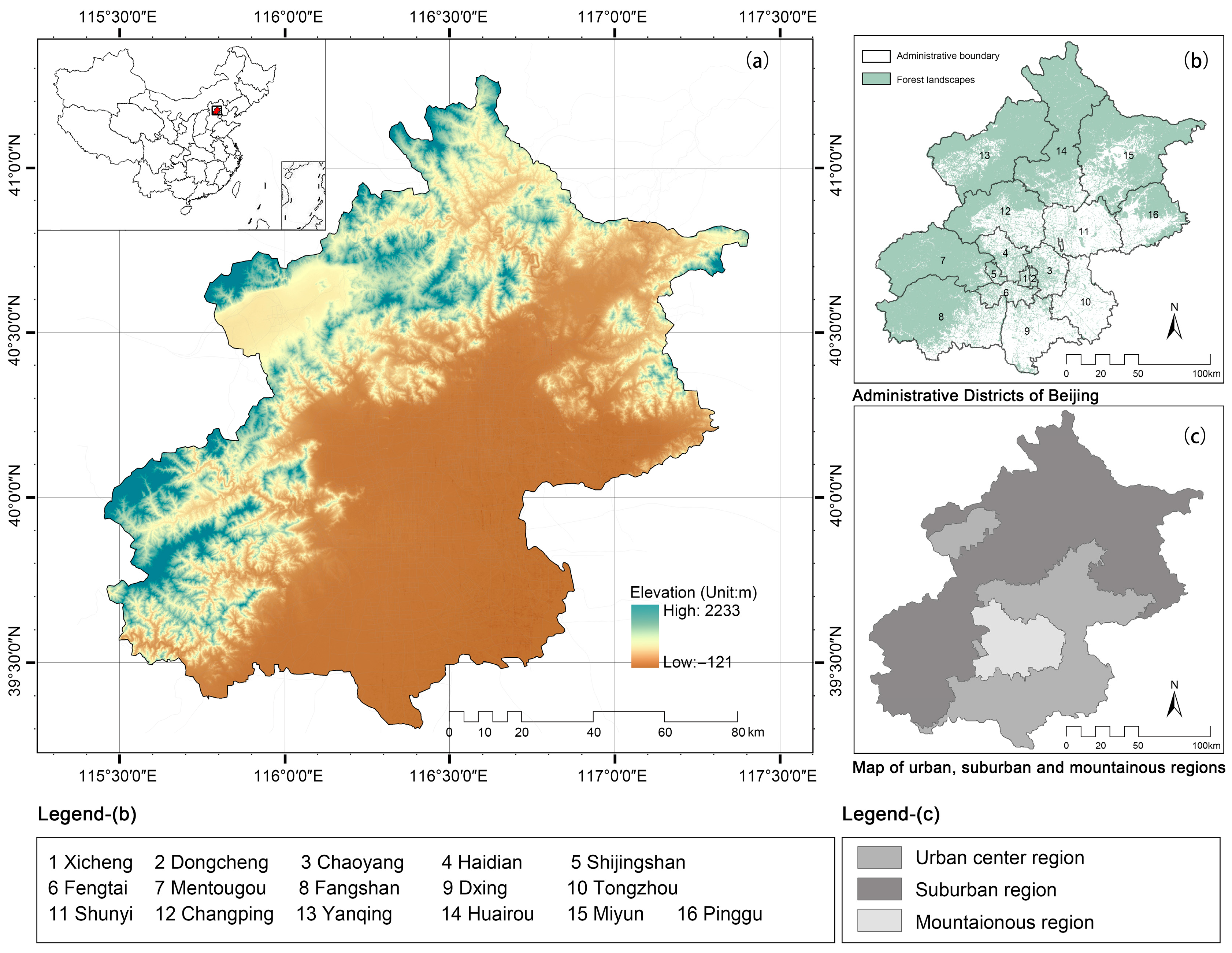
Beijing is located in the northwestern part of the North China Plain (115°25′–117°30′ E, 39°28′–41°05′ N), and presents a characteristic semi-humid continental monsoon climate. Encompassing a total area of 16,410 km2, the city is surrounded by mountains to the north, northeast, and west, boasting abundant forests and high species diversity. The central part is a vast plain area, where a high level of urbanization has led to the fragmentation of forest landscapes (Figure 2). Because Beijing is a megacity, the urbanization and development of the city has seriously affected the landscape structure and maintenance of biodiversity of these forests.
The data sources employed in this paper were as follows: First, the land use data for the year 2020, with a spatial resolution of 10 × 10 m, was acquired from the global surface coverage products offered by the European Space Agency. The data can be accessed on the website https://esa-worldcover.org/en, accessed on 24 November 2021). We used Google Earth Pro and SAS Planet software to obtain 10 m resolution satellite remote sensing image data of Beijing in 2005. The detailed process involved using Google Earth Pro software to cache the historical remote sensing images of Beijing in 2005, followed by reading and loading the cached images using SAS Planet software. Subsequently, we completed the mosaic preservation and download of the remote sensing images. ENVI software was used to interpret remote sensing image data after radiometric calibration, atmospheric correction, image mosaic, geometric correction, and cutting. The accuracy is 92.7%. Taking into account the actual land resource utilization in the study area, we classified the land use types into six distinct categories: forest land, cultivated land, grassland, water, urbanized land, and unused land. Considering the scope of the study and available computing power, we resampled these data to a resolution of 30 m. Next, the net primary productivity (NPP) data for the year 2020, with a spatial resolution of 30 × 30 m, were acquired from the Geographic Remote Sensing Ecological Platform. The data can be accessed on the website http://www.gisrs.cn/, accessed on 24 November 2021. Thirdly, the national monthly average temperature and precipitation datasets for the year 2020, with a spatial resolution of 1 km, were obtained from the National Science and Technology Infrastructure. The data can be accessed on the website http://data.tpdc.ac.cn/zh-hans/, accessed on 15 November 2021. Fourthly, the digital elevation model (DEM) data, with a spatial resolution of 30 m, were sourced from the Geospatial Data Cloud Platform. The data can be accessed on the website http://www.gscloud.cn/, accessed on 15 November 2021. Fifthly, the road vector data, including railway, primary road, and secondary road, were acquired from the Resource and Environment Science and Data Center. The data can be accessed on the website: http://www.resdc.cn, accessed on 15 November 2021. Lastly, the nighttime light intensity data for the year 2020 were acquired from the National Environmental Information Center of the United States National Oceanic and Atmospheric Administration.

2.2. Methods

2.2.1. Construction of Biodiversity Potentiality Evaluation Model

Habitat quality refers to the combined impact of external threats’ intensity and the inherent vulnerability of ecosystem types to threats, influencing biodiversity. That is, habitat quality can be used to quantify the effects of human activity factors on the living environment of any species in a particular spatial range. High-carbon forests can provide obvious advantages in effectively mitigating climate change, promoting biodiversity by alleviating the heat island effect, and regulating temperature and humidity in a city. Therefore, we selected habitat quality and carbon sink as vital ecosystem services that were used to evaluate the BMC of forest landscapes. Based on questionnaire responses from 15 experts and hierarchical analysis, the weight coefficients of habitat quality and carbon sink were determined (See Table S1 and Figure S1 in the supporting document for the process of weight coefficients determination). The calculation formula for the BMC is as follows:
B M C = 0.43 C S S D + 0.57 H Q S D ,
where CSSD is the standardized carbon sink value of each grid unit and HQSD is the standardized habitat quality value of each grid unit. The standardization was performed using the Min–Max normalization method. The specific calculation formula for Min–Max standardization is as follows:
x S D = x x m i n x m a x x m i n ,
where, x S D represents the standardized value, x represents the original data value, xmin represents the minimum value of the original data, and xmax represents the maximum value of the original data.
(1)
Carbon sink model
Net Ecosystem Productivity (NEP) is the portion of Net Primary Productivity (NPP) that remains after subtracting the respiration of heterotrophic organisms [53]. Specifically, soil heterotrophic respiration reflects the value of the net carbon exchange and carbon sink in terrestrial ecosystems [54], which can be quantitatively described as the carbon sink potential of the ecosystem [55]. Soil heterotrophic respiration was computed based on the methods of Liu et al. [56], utilizing Equations (3)–(5):
N E P = N P P R h
R h = 0.6163 R s 0.7918
R s = 1.55 e 0.031 T × P P + 0.68 × S O C S O C + 2.23 ,
where NEP represents net ecosystem productivity (kgC·m−2·a−1), NPP represents net primary productivity (kgC·m−2·a−1), R h represents soil heterotrophic respiration (kgC·m−2·a−1), R s represents soil respiration (kgC·m−2·a−1), P represents annual precipitation (m), T represents annual average temperature (°C), and SOC represents the carbon density of the 0–20 cm surface soil. The SOC value, based on the findings of Xu et al. (2019) [57], is determined to be 4.12 kgC/m2.
(2)
Habitat quality model
The assessment of habitat quality for forest landscapes was conducted using the InVEST model. Drawing upon the specific conditions of the study area and pertinent research findings [58,59,60], we selected cultivated land, urbanized land, railways, primary roads, and secondary roads as the threat factors. Primary roads include national expressways and provincial highways, and secondary roads refer to urban arteries. Then, we set three threat factor parameters, including the maximum effect distance (drmax), the threat weight (wr), and the distance–decay function according to the model manual and existing findings of Lv et al. [36], Sallustio et al. [61], Gong et al. [62], and Song et al. [63]. The specific settings of the parameters are shown in Table 1. The calculation of habitat quality involved the utilization of the following formula:
Q x t = H t 1 D x t z D x t z + k z ,
where Q x t represents the habitat quality of grid unit x in land use type t; H t signifies the habitat suitability of land use type t; k represents the half-saturation constant, which can be determined through model execution; z is a scaling parameter with a fixed value of 0.5, and Dxt represents the threat degree of grid unit x in land use type t; and was calculated using Equation (7):
D x t = r = 1 R y = 1 Y r w r r = 1 R w r r y i r x y β x S t r ,
where R is the number of threat factors; wr represents the effective weight of each threat factor; Yr means the set of grid cells of the threat factor layer in the land use/cover map; ry denotes the number of threat factors in the unit grid of a land use type; βx is the accessibility of grid cell x; Str represents the sensitivity of land use type t to threat factor r; and irxy is expressed as a linear or exponential function of the distance from the threat source to the habitat. This was calculated using Equations (8) and (9):
i r x y = 1 d x y d r m a x   i f   l i n e a r
i r x y = e x p 2.99 d x y d r m a x   i f   e x p o n e n t i a l ,
where dxy represents the linear distance between grid units x and y, while drmax indicates the maximum influence distance of threat factor r.

2.2.2. Selection and Calculation of Landscape Pattern Indices

Drawing on the context of Beijing and relevant studies [48,64,65], we selected a set of 20 commonly used landscape indices that capture various aspects such as area and edge, shape, aggregation, and diversity (See Table S2 in the supporting document for landscape indices descriptions). However, the multicollinearity caused by the overlapping of some indices affects the accuracy of regression results. Therefore, according to the selection criteria proposed by Su et al. [66], we conducted Pearson correlation analysis on these 20 landscape indices and retained the indices with a correlation coefficient |r| > 0.9 through a two-tailed test (see Table S3 in the supporting document for correlation analysis results of 20 landscape indices). Finally, the IJI, CONNECT, PRD and the CIRCLE_MN were selected. IJI is a measure of isolating the intermixing or juxtaposition of patch types. It reflects the isolated distribution of different patch types. The smaller the value, the more adjacent the patch is to the same patch type and the less adjacent to other patch types. CONNECT quantifies the degree of functional connectivity between patches of the same type. It acts as a rough proxy for connectivity within the form samples. PRD is calculated as the ratio of the count of patch types within the landscape boundary to the total landscape area, which provides an assessment of landscape diversity. CIRCLE_MN calculates the ratio of patch area to the minimum outer circle of the patch, indicating the compactness of the landscape. After verification by the ordinary least squares method (OLS), the variance inflation factor of each variable was less than 7.5, indicating no multicollinearity remained. The moving window analysis method was used to quantify the local landscape patterns. If the search window size is a multiple of the pixel size, the error is small [67]. We selected 90 m, 180 m, 270 m, 360 m, 450 m, and 540 m as window sizes for analysis. When the search window size is 360 m, the change in each index curve gradually tends to be gentle, indicating that this size can retain the variation characteristics of landscape patterns.

2.2.3. Spatial Autocorrelation Analysis

Spatial autocorrelation refers to the examination of the spatial interaction between neighboring regions to understand the relationships of specific geographical phenomena. It encompasses global spatial autocorrelation and local autocorrelation [68]. The global Moran’s I was utilized to assess the spatial clustering of BMC across the entire study area. Geoda software was employed to perform this analysis. The range of Moran’s I value is from −1 to 1, where its absolute value indicates the degree of correlation. When the value is close to 0, this indicates a random distribution of BMC. The calculation formula is:
I = i = 1 n j = 1 n w i j x i x ¯ x j x ¯ S 2 i = 1 n j = 1 n w i j ,
where n represents the count of patches in the study area. Wij denotes the spatial weight matrix, and xi and xj represent the BMC values of regions i and j, respectively. x ¯ signifies the average BMC value, and S2 denotes the variance of the BMC values.
Local spatial autocorrelation reveals the similarity between a regional unit and its neighborhood, which explains spatial heterogeneity [69]. The Local Indicators of Spatial Association (LISA) diagram commonly characterizes the spatial aggregation position. A positive local spatial correlation is indicated when the LISA coefficient is greater than 0, suggesting a “High–High” or “Low–Low” spatial aggregation type. Conversely, a negative local spatial correlation is indicated when the value is less than 0, indicating a “High–Low” or “Low–High” spatial aggregation type. In this study, the single variable local autocorrelation was used to reflect the spatial aggregation characteristics of BMC values.

2.2.4. Geographical Weighted Regression Analysis

A geographic weighted regression (GWR) model is effective for addressing spatial heterogeneity in regression analysis. This type of model can be used to calculate the regression coefficient of each unit and construct a local regression equation to accurately describe the spatial relationship between variables. The model is expressed as Equation (11):
y i = β 0 m i , n i + k = 1 P β k m i , n i x i k + ε i ,
where (mi,ni) is the geographical coordinate of the ith sample unit, β0 (mi,ni) is the intercept of the ith sample, βk (mi,ni) is the local estimated coefficient of independent variable xik, and εi is a random error term.
In this study, the BMC of forest landscapes was used as the dependent variable, and the four indices representing landscape intermixing, connectivity, diversity, and compactness were used as the dependent variables to construct OSL and GWR regression models. The adaptive approach was employed to determine the spatial weights, while the corrected Akaike Information Criterion (AICc) was utilized to identify the optimal bandwidth. The diagnostic results indicate that the GWR model outperformed the OLS model, as evidenced by a higher adjusted R2 and an AICc value < 3, suggesting better explanatory power of the GWR model in comparison to the OLS model (Table 2). Street and township-level data were employed to demarcate the study area and examine the variations in landscape patterns across different regions. Additionally, these data were utilized to explore the driving mechanisms of these patterns on the BMC of forest landscapes.

3. Results

3.1. Land Use Structure Change

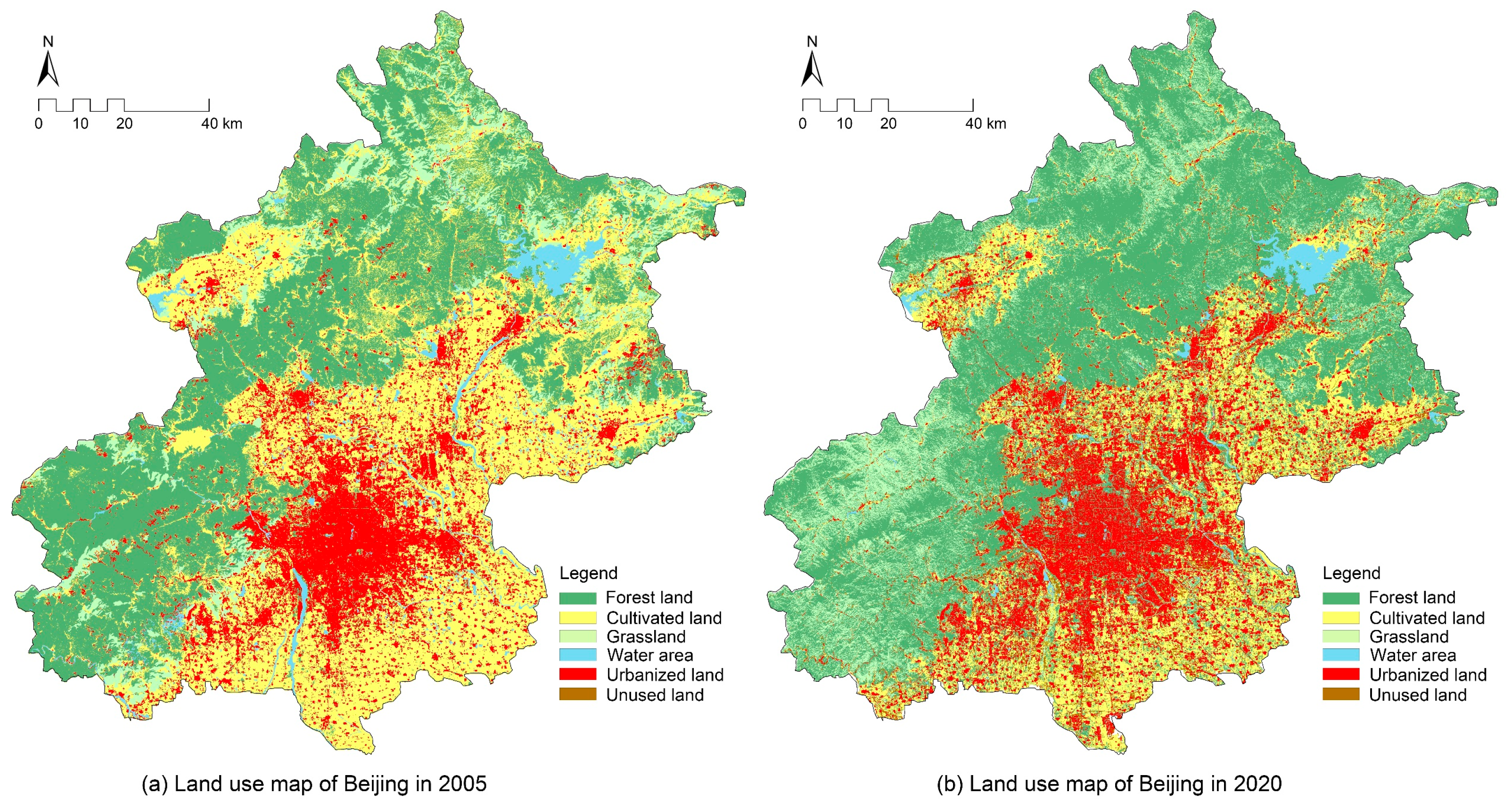
Figure 3 illustrates the predominant land use types in Beijing in 2005 and 2020, including forest land, cultivated land, and urbanized land. From 2005 to 2020, the three proportions changed as follows 36.53% to 47.86%, 37.55% to 18.02%, and 14.85% to 15.36%, respectively, accounting for 88.93% to 81.24% of the total area. According to Table 3, it can be seen that during this period there was a land use change area of 6755.11 km2, comprising 41.16% of the total area. The loss of cultivated land was the most significant, with a decrease of 2081.14 km2, and was mainly transformed into forest land, grassland, and unused land. The net increase in those three was 1850.37 km2, 775.59 km2, and 554.64 km2, respectively, which benefited from the Returning Farmland to Forest as well as the Afforestation and Greening projects. The urbanized land area remained relatively stable, with a net increase of 161.91 km2. The transformation from cultivated land represented 88.11% of the total change, indicating that the rapid expansion of urban areas and population increase have led to the loss of marginal cultivated land and intensified the land supply-demand imbalance. The water area experienced a decrease of 261.47 km2, with conversions into other land cover types such as cultivated land, forest land, and grassland, accounting for transfer ratios of 32.87%, 29.39%, and 18.89% respectively.

3.2. Patterns and Changes for the BMC of Forest Landscapes

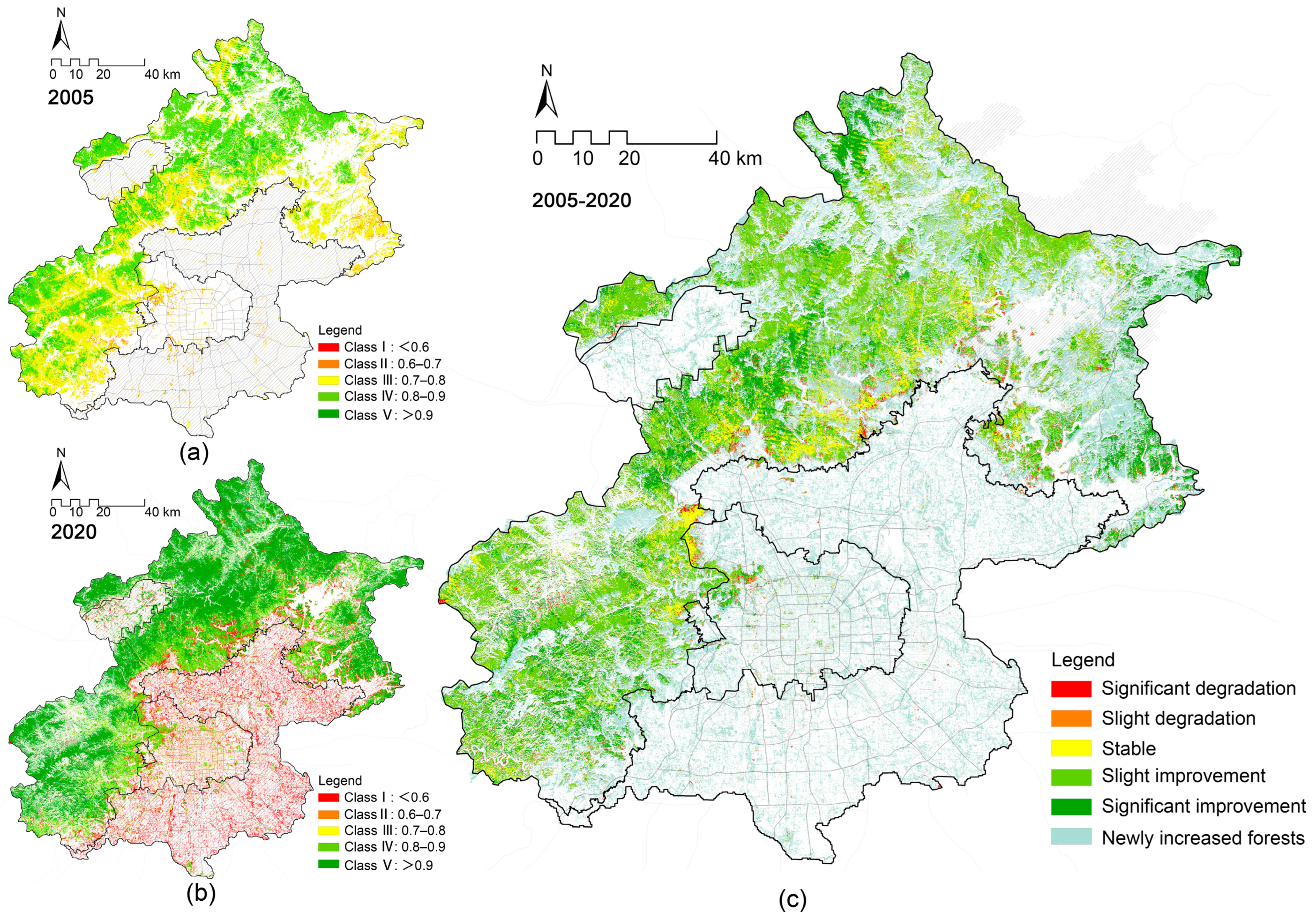
After 15 years of large-scale afforestation, the BMC of forest landscapes has improved, with an average value rising from 0.798 to 0.822, indicating that the environment restoration capacity and ecosystem service function have been enhanced. However, due to differences in the levels of urbanization, the BMC showed significant spatial heterogeneity. To facilitate the analysis of specific changes, the BMC was categorized into five classes using the natural breakpoint method: Class I (<0.6), Class II (0.6–0.7), Class III (0.7–0.8), Class IV (0.8–0.9), and Class V (>0.9). It can be seen from Table 4 that the proportion of classes I and V increased significantly from 2005 to 2020. In 2005, the areas of classes I and II accounted for only 3.55% and were mainly distributed in urban centers, showing a gradual decrease along the urban–rural gradient. Class III and IV areas accounted for 46.95% and 47.59% of the total area, respectively, and were primarily situated in the mountainous region. In 2020, the Class I area increased by 16.85%, due to the large scale of newly developed forests with low values in urban and suburban regions. The BMC of classes IV and V BMC constituted 80.40% of the overall forest area and were concentrated in the western and northern mountains.
Figure 4 and Table 5 show the spatial pattern change of BMC. Areas that remained at the same class during the study period were considered stable, while those that varied between consecutive classes were considered to exhibit slightly improved or decreased BMC. Those areas that underwent dramatic changes across multiple grades were considered to be significantly improved or decreased. The total transferred area was 4650.57 km2, of which the stable area was 550.25 km2, accounting for 11.83%; this type of area was located in the mountainous region with a low intensity of human disturbance. Areas of 36.02 km2 in the urban center and suburbs experienced a slight decline, accounting for 0.77% of the total area. The transition zone between plain and mountainous areas experienced a significant decline, with an area of 151.44 km2, accounting for 3.26% of the total area. In addition, 60.46% and 23.68% of the areas experienced slight and significant improvement in BMC, in the mountainous areas with low accessibility, at high elevations, or with steep slopes. In addition, areas experiencing a slight or significant improvement were scattered in urban and suburban regions.

3.3. Landscape Patterns Change

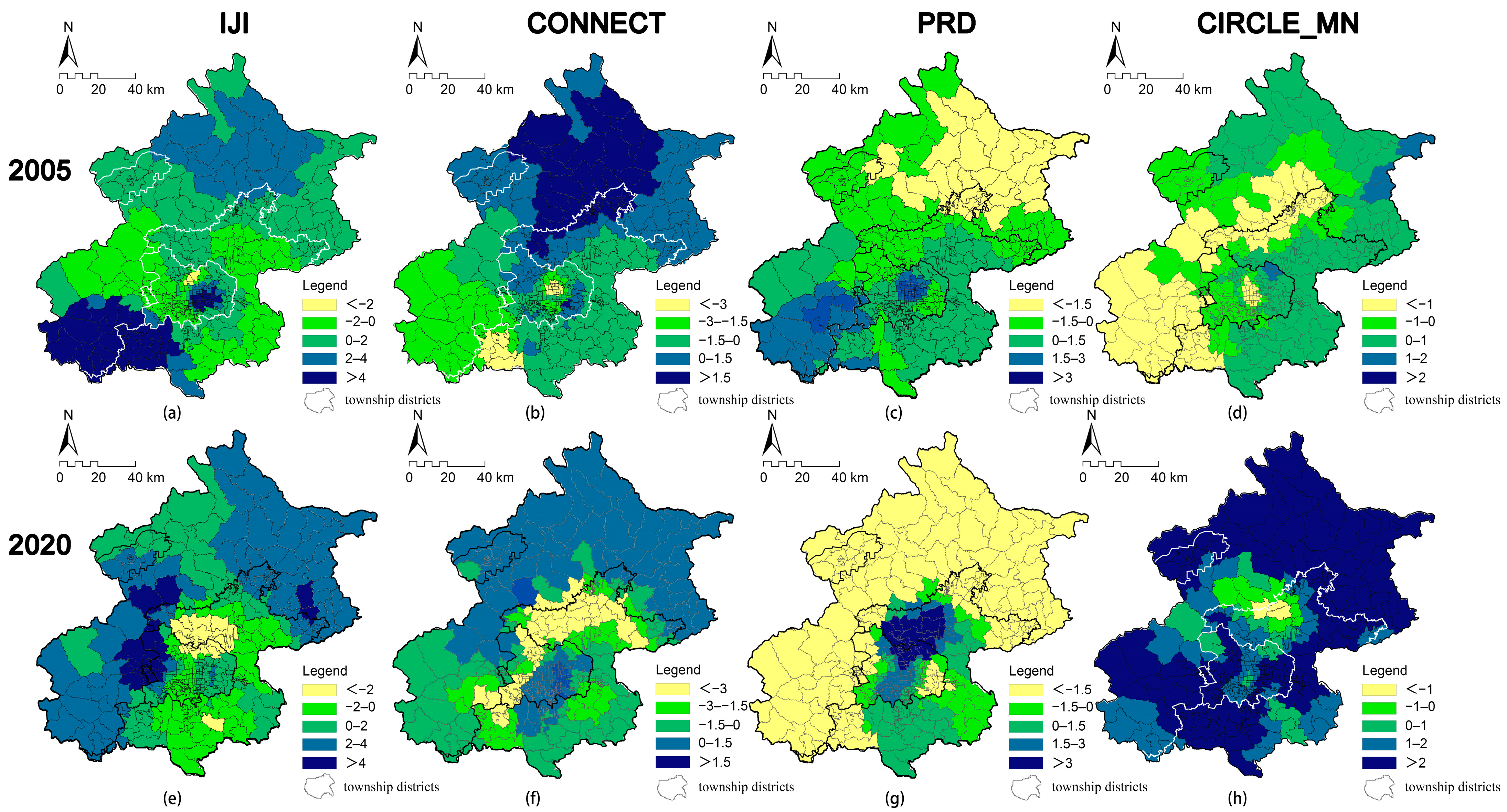
Figure 5 depicts the landscape pattern variations and transformations in the urban, suburban, and mountainous areas of Beijing over the past 15 years. The IJI shows that, in 2005, landscape intermixing was high in the urban region, medium in the mountainous region, and low in the suburban region. By 2020, the landscape intermixing of the urban center as well as in the northwestern and southwestern mountainous regions had decreased significantly. In contrast, the landscape intermixing in the suburban region increased had transformed into a multi-type aggregation pattern. The CONNECT shows that, in 2005, low values existed in the urban center, the southeastern suburban plain, and western mountainous regions. By 2020, the spatial extent of the low-value CONNECT area had been greatly reduced, and the connectivity of the urban center and the western mountainous region had been significantly improved, reflecting that the trend of landscape spatial fragmentation has been alleviated. The PRD shows that, in 2005, the landscape diversity was low in the urban center, the southeastern suburban region, and the western mountainous region. The diversity was high in the northern mountainous region and the southwest suburban region. By 2020, noticeable expansion of high-value areas was observed, particularly in the suburban region, signifying an augmentation in landscape diversity and complexity, along with a reduction in the disparity of area proportions. However, the city center continued to have a low value of PRD. For the CIRCLE_MN, in 2005, low-value areas were predominantly concentrated in the urban center, whereas high-value areas were primarily situated in peri-urban suburbs and northern mountainous regions. By 2020, the compactness of the urban center and the southwestern mountainous regions had increased slightly, reflecting a gradual regularization of the patches. The compactness of the suburban region had declined, indicating a more natural transformation of the patches. In general, from 2005 to 2020, the landscape intermixing decreased, and the diversity, compactness, and connectivity increased in the urban center. The landscape compactness decreased while the connectivity, intermixing, and diversity improved in the suburban region. In the mountainous region, the landscape intermixing decreased while the connectivity and diversity increased, and the compactness remained unchanged.

3.4. Spatial Autocorrelation Analysis Results of the BMC of Forest Landscapes

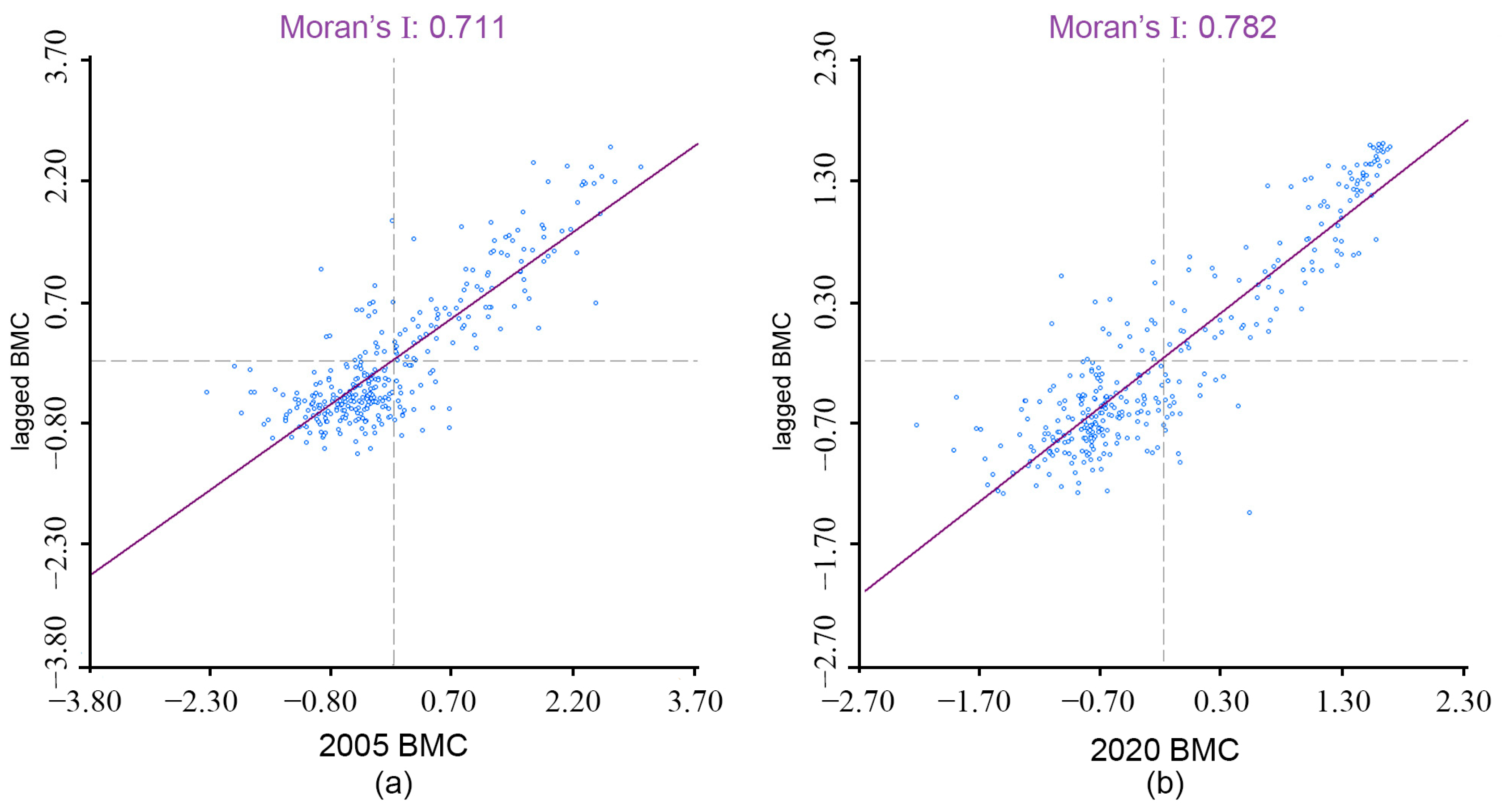
To further investigate the spatial pattern of the BMC of forest landscapes, an analysis of the global and local spatial autocorrelation of BMC was conducted. The findings of the global autocorrelation analysis are depicted in Figure 6, revealing global Moran’s I indices of 0.711 in 2005 and 0.782 in 2020. The data points were predominantly located in the first and third quadrants, indicating that BMC was positively correlated in spatial distribution and showed spatial bipolar agglomeration. Specifically, districts with high BMC tended to be aggregated with surrounding districts with high BMC, while districts with low BMC tended to be aggregated with surrounding districts with low BMC.
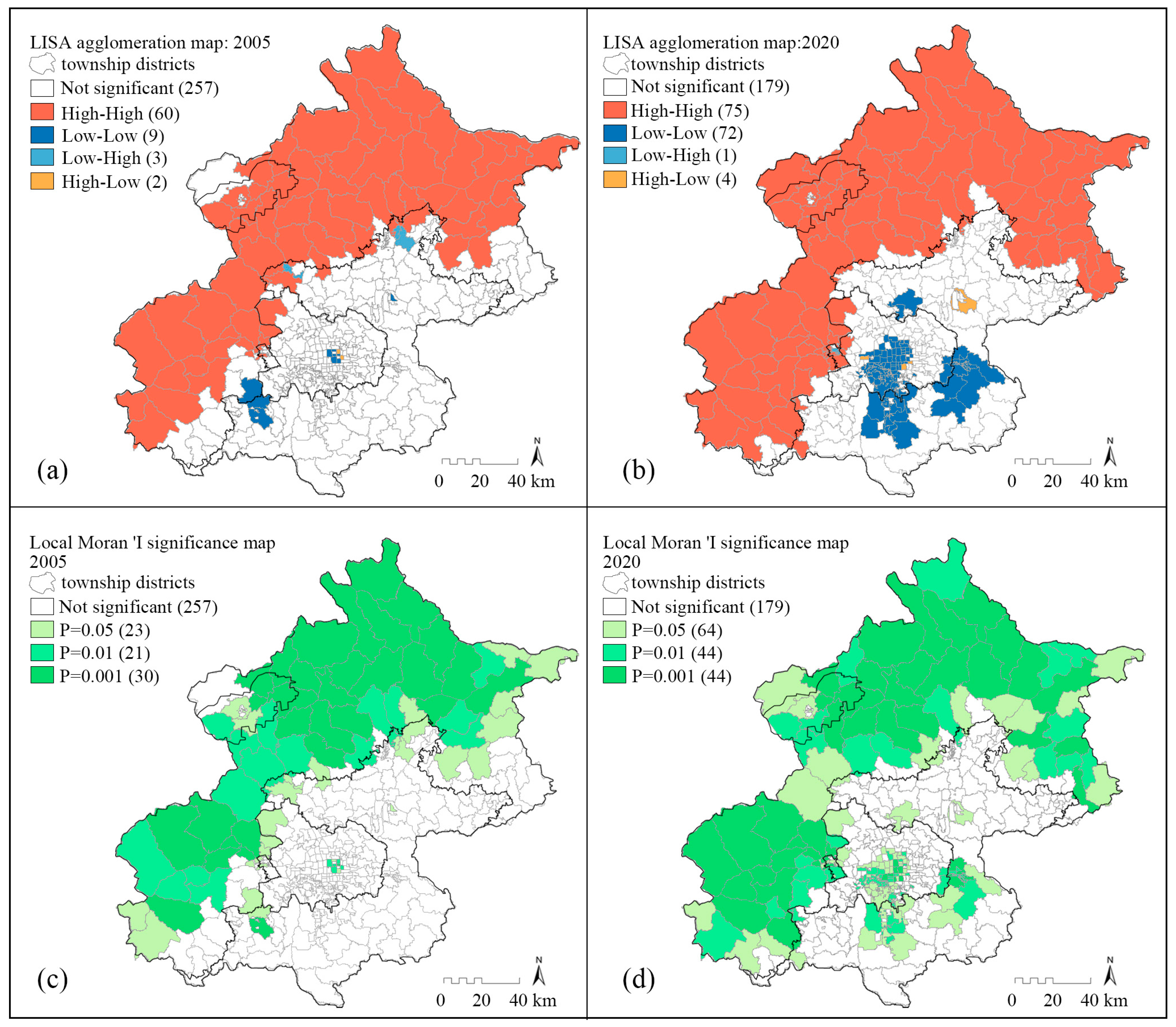
The local spatial agglomeration characteristics of BMC values were analyzed based on the LISA clustering map. The results showed that all districts could be divided into five types: high-value districts adjacent to neighboring high-value districts (H-H), low-value districts adjacent to neighboring low-value districts (L-L), high-value districts adjacent to neighboring low-value districts (H-L), low-value districts adjacent to neighboring high-value districts (L-H), and districts with no significant difference in values (Figure 7). Throughout the study period, the H-H areas were predominantly distributed in the mountainous region, with numerous nature reserves and national forest parks belonging to restricted development zones (See Figure S2 in the supporting document for spatial distribution of nature reserves and forest parks). The L-L areas increased significantly, mainly in the urban region with high density urbanization and southern and southeastern peri-urban suburbs that were greatly affected by human disturbance. The H-L and L-H areas showed a sporadic distribution. Overall, the forest landscapes with the most significant spatial correlation of BMC were predominantly distributed in the urban and mountainous regions due to the differences in the degree of urbanization caused by economic development. Finally, the global and local spatial autocorrelation of BMC value was tested by Monte Carlo simulation testing. The results indicated that the p value was <0.001, the Z score was higher than 2.58, and the BMC had characteristics of significant spatial correlation and aggregation, with a confidence level of 99.9%.

3.5. Effects of Landscape Patterns on the BMC of Forest Landscapes

The geographic weighted regression results are shown below in Figure 8 and Table 6. The results of IJI show that, in 2005, landscape intermixing was spatially unstable with intense urbanization. Whether in rural or large-scale urban areas, the positive effect of intermixing was very significant. In contrast, the negative effects of intermixing on BMC in peri-urban suburbs were evident. By 2020, in the urban region, the effects of landscape intermixing on the BMC had changed from positive to negative. The negative effects in the northern peri-urban suburbs had increased significantly. The mountainous region and outer suburbs were the main areas of positive correlation, and the intensity and scope of positive effects had increased. In general, in areas with high or low values of BMC, IJI was positively correlated with BMC. In areas with moderate BMC values, IJI was negatively correlated with BMC.
The results of CONNECT show that, in 2005, landscape connectivity positively affected the BMC in the northern outer suburbs and mountainous regions, while it negatively affected the BMC in the urban center and southwestern mountainous areas. By 2020, in the urban region, the effects of landscape connectivity on BMC had changed from negative to positive. However, the scope and intensity of the negative effects on the BMC in northern peri-urban suburbs had increased significantly. Overall, connectivity analysis shows a significant positive effect in the northern mountainous regions and fluctuations in the intensity and scope in urban and suburban regions that experienced intensive human disturbance.
The results of PRD show that, in 2005, landscape diversity had a significant positive effect on BMC in the urban and southwestern mountainous regions and a predominantly negative effect on northern mountainous regions and outer suburbs. By 2020, the negative effect on the scope and intensity of landscape diversity on BMC in mountainous and suburban regions increased significantly, and the positive effect on the scope and intensity of BMC in the northern peri-urban suburbs increased significantly. Overall, diversity had a strong positive effect on BMC in urban and peri-urban areas, with urbanized land as the matrix. For large and intact forest landscapes, the negative effect was more significant.
The results of CIRCLE_ MN show that in the past 15 years, due to the changes in land use patterns in Beijing, the scope and intensity of landscape compactness also fluctuated wildly. In 2005, the landscape compactness reduced the BMC in the urban center and the southwestern mountainous regions, while it positively affected the BMC in the northern mountainous regions and the eastern suburbs. By 2020, the positive effects of landscape compactness on BMC increased significantly in scope and intensity, with only the northern peri-urban suburbs showing a negative effect.

4. Discussion

4.1. Spatial and Temporal Changes of the BMC and Landscape Patterns in Beijing

As an important city in northern China, Beijing experienced rapid urbanization and ecological development in the early years of the 21st century [70]. The forest landscape is the most critical habitat for protecting biodiversity and maintaining ecosystem services. These forests are subject to increased levels of environmental threats during urbanization, which has had a negative effect on BMC and gradually decreased with the urban–rural gradient in Beijing. At the same time, large-scale ecological planning efforts and policy interventions have protected more ecological spaces, restricted the expansion of urbanized land, and increased forest area, enhancing the overall BMC.
In this context, the landscape pattern of Beijing has also undergone significant changes. First, the average value of IJI decreased by 11.45%, indicating that the overall landscape intermixing decreased. The landscape intermixing in the northwestern and southwestern mountainous regions decreased significantly because the Returning Farmland to Forest Project along with Afforestation and Greening projects have promoted a significant increase in forest area [71] and a decrease in the diversity of landscape types. The intermixing of the urban center has increased significantly because the multi-scale green spaces such as urban greenways, pocket parks, and forest parks have dispersed the concentrated urbanized land [72]. In the suburban region, as a result of and the conversion of large-scale cultivated land into forest land, the landscape is now characterized by multi-type aggregation, and the intermixing has increased. In many other countries, particularly in Latin America, urban development over the past few decades has been characterized by urbanization, expansion of agricultural land, and encroachment into protected areas. The main challenge faced by landscapes is forest conservation. da Silva et al. [73] assessed forest landscapes in the Atibaia River basin, which connects the important cities and economic centers of São Paulo and Campinas in Brazil. They found that it is crucial to consider the land use patterns surrounding forest fragments to determine the permeability that ensures both material and energy flows between the remnants. Additionally, other factors such as matrix permeability, terrain characteristics, and species’ responses to these structural features need to be evaluated.
Second, the average CONNECT_MN increased by 64.28%, indicating a significant increase in overall landscape connectivity and a close link between all land use types. This was primarily because Beijing has established a global territorial spatial development and protection pattern in recent years. This has been accomplished through detailed land use planning adjustment which continues to promote a reduction in the urbanization rate of urban and rural and efficient use of land resources [66]. Vanderley-Silva et al. [74] studied the forest landscapes of the Green Belt Biosphere Reserve in São Paulo and employed a multicriteria evaluation approach to verify the benefits of enhancing forest connectivity and avoiding the clustering of high-density urban land uses. Their findings showed that improving connectivity not only facilitated resource utilization and habitat establishment but also promoted plant gene flow and animal migration. Additionally, factors such as altitude and proximity between forest remnants were identified as important considerations in determining the highest priority conservation areas, which is consistent with the results of our study. Han et al. [32]. explored the relationship between forest remnants and new green spaces in southern Seoul, South Korea, and made an intriguing discovery. They found that the spatial arrangement of patches may play a more significant role in species survival than patch size when less than 30% of a specific habitat type remains fragmented in the landscape. However, currently, most forest patches at the urban edge are protected as part of green belts, while smaller patches receive minimal to no protection. Therefore, it is increasingly important to consider scattered forest remnants as essential components and incorporate them into conservation plans when developing urban green infrastructure. The actual measures taken in Beijing’s urban forest conservation planning validate the significance of these research findings.
Third, the average value of PRD increased by 55.44%, indicating that the overall landscape diversity has improved. However, the urban center is always a low-value area, because urbanized land dominates and there are fewer types of landscape present. In contrast, the landscape diversity in the suburban region has increased significantly because the urbanization process and the environmental protection projects have led to a significant fluctuation in landscape types. In addition, more forest land, cultivated land, and water bodies are predominantly located in the suburban regions, and the landscape types are more abundant. According to the land use transfer matrix, there is a decreasing trend in water bodies compared to forest landscapes, primarily due to their conversion into agricultural land, forest land, and unused land. First and foremost, Beijing faces the challenge of relatively scarce water resources, leading to a long-standing issue of water supply–demand imbalance [75]. To meet the needs of urban development and residents’ water consumption, Beijing extensively relies on water transfers from surrounding areas, including water diversion and groundwater extraction [76]. These excessive practices of water resource exploitation have resulted in declining water levels in rivers and lakes, consequently reducing the area of water bodies [77]. Moreover, in recent years, Beijing has experienced reduced rainfall and increased drought conditions due to climate change, further exacerbating the pressure on water resource availability. Decreased rainfall has led to diminished water levels in rivers and lakes, resulting in a corresponding decrease in water body areas [78]. The degraded water bodies have mainly been transformed into agricultural land and unused land. Additionally, extensive afforestation projects have been undertaken in Beijing to enhance vegetation coverage and improve ecosystem functions. Consequently, some water bodies have been transformed into forest land. These forest land projects encompass urban forests, forest parks, wetland parks, and other initiatives that aim to improve the ecological and living environments [79]. It is important to note that these projects undergo rigorous planning and assessment to ensure the protection and sustainable utilization of water bodies, maintaining overall ecosystem stability, and addressing challenges such as water scarcity and pollution.
Fourth, in terms of compactness, due to the more refined land use planning and control in the urban center [80], the CIRCLE_MN value has increased slightly, reflecting that the patches have become more regular. In the suburbs, landscape compactness has declined, mainly because regular farmland has been replaced by natural forest land and scattered towns.

4.2. Driving Mechanism of Landscape Pattern on the BMC of Forest Landscapes

Understanding the changes in the capacity of a system to maintain biodiversity across time and space and the driving mechanism of that change is crucial for effective ecosystem management and can alleviate the enormous pressure of urban expansion on ecological protection efforts [48,81]. As the most essential and fundamental component of urban ecosystem services, the effects of landscape patterns on the ecological function of forest landscapes should not be ignored during the process of rapid urbanization [82].
Overall, from 2005 to 2020, the effects of the four attributes of landscape pattern on the BMC of forest landscapes showed significant differences. Landscape compactness had the greatest effect, followed by landscape diversity, intermixing, and connectivity. First, in areas with high values of BMC, landscape compactness showed a positive effect because higher compactness increased the resistance of forests to negative factors [64]. For areas with low values of BMC, a decrease in landscape compactness means a decline in the density of urbanized or cultivated land, which benefits the improvement of BMC. As pointed out by Moro and Milan [83], both patch area and compactness are crucial because dispersed forest patches are more susceptible to the influence of external factors, including increased wind and solar radiation incidence, decreased humidity and microclimate changes, alterations in species distribution and abundance, increased vulnerability to invasive species, and loss of gene flow. These disturbances, known as edge effects, result from a combination of natural and anthropic factors that operate in the boundary zones between patches and their surroundings, ultimately affecting internal ecological processes [84].
Second, landscape diversity has a positive effect on the BMC in the urban center and peri-urban suburbs because the increase in diversity can alleviate the ecological pressure brought by high-density urbanized land, which is in line with the research results of Li et al. [40] and Zhu et al. [14]. In contrast, in areas with high values of BMC, an increase in landscape diversity may expand the negative effects of human disturbance, thus reducing BMC. For areas with medium values of BMC, with the strengthening of policy intervention, the stress effects of urban expansion would be effectively controlled, and the positive benefits of landscape diversity gradually increases. The identification of land use and occupation around forest patches enables the assessment of the intensity of external environmental pressures exerted on the remaining forest fragments. Previous studies have revealed that a significant portion of forest fragments is surrounded by extensively modified areas, including deforested and/or degraded regions, roads, exposed soil, and buildings. The widespread conversion of land for urbanization and agricultural purposes may disrupt forest ecosystems and impact the size of the fragments [85].
Third, in the urban center, landscape intermixing positively affects BMC because an increase in intermixing means that the spatial relationship between urbanized land and other ecological land is relatively balanced. In contrast, landscape intermixing harms BMC in suburban and mountainous regions, because increased intermixing reduces the scale effects of high-quality forests. With the development of urbanization, the negative effects of intermixing on BMC in peri-urban areas gradually expands. This is consistent with the findings put forward by Han et al. that ecosystem services provided by natural habitat fragments to adjacent areas may follow a distance-dependent pattern, whereby fragments in close proximity to high-density residential areas often exhibit lower habitat quality compared to fragments closer to the urban edge covered by primary forest [32].
Fourth, enhancing landscape connectivity in the urban center leads to a significant improvement in BMC. The spatial configuration and degree of isolation of habitats are important variables, particularly in urban landscapes with few forest fragments [74,86]. These small forest fragments play an essential role in landscape connectivity as they serve as steppingstones, refuges, or sources of forest nucleation, which help ensure biotic movement and accelerate recovery processes [73]. In recent years, the development of urban park rings, greenways, and micro-green spaces in Beijing has improved the connectivity of forest landscapes. This development is conducive to improving the success rate of biological migration [87]. For the northern peri-urban suburbs, the negative effects of the expansion of urbanized land are far more significant than the positive effects of policy intervention on ecological protection. In the southwestern mountainous areas, landscape connectivity has a minor positive impact on BMC, primarily attributed to the extensive conversion of grassland and cultivated land into forest land facilitated by initiatives such as the Three-North Shelterbelt and the Afforestation and Greening projects [88]. The sensitivity of BMC to connectivity in other regions was not significant.

5. Conclusions

This study investigated the specific driving mechanism of landscape patterns on BMC of forest landscapes. By evaluating the BMC of forest landscapes and four typical landscape pattern indices, this study used spatial correlation analysis and geographic weighted regression models to explore the driving mechanism of landscape pattern characteristics on the BMC of Beijing’s forests. Our findings could serve as a valuable resource for future urban biodiversity conservation planning and the sustainable development of forest landscapes in Beijing. The main conclusions are as follows:
(1)
The overall BMC of forest landscapes in Beijing improved from 2005 to 2020, with the average value rising from 0.798 to 0.822. In the urban center and suburban regions, 36.02 km2 of forests experienced a slight decline. In the transition zone connecting suburban and mountainous regions, about 3.26% of forests experienced a significant decline. Increasing the aggregation of high-quality, healthy, and stable forests is critical to preventing landscape fragmentation and promoting material cycling and capacity flow. In the mountainous region with a low intensity of human disturbance and high elevation, about 11.83% of forests remained stable, and 60.46% and 23.68% of the forests experienced slight and significant improvement, respectively. It is necessary to strengthen the management of nature reserves, build a biodiversity conservation network, and limit the encroachment of human activities on ecologically fragile and sensitive areas.
(2)
The landscape pattern changed significantly from 2005 to 2020 in Beijing. As a whole, landscape intermixing and compactness decreased slightly by 11.45% and 7.82%, while landscape connectivity and diversity increased significantly by 64.28% and 55.44%, respectively. In the mountainous region, the intermixing of the landscape decreased significantly, while the diversity and connectivity increased. It shows that the overall landscape pattern of the mountainous area has improved. In future planning and development, it is necessary to continuously strengthen ecological conservation and restoration to reduce landscape diversity and confounding. At the same time, measures such as artificial afforestation, hill-closing afforestation, young growth tending, and low-quality forest transformation should be taken to ensure that the ecological function remain unchanged. In the suburban region, the landscape compactness decreased across a wide range, while the intermixing, diversity, and connectivity increased. The urban green belt dominated by forest land can actively promote the transformation of construction space to ecological space, avoid the reduction in ecological space area caused by disorderly urban expansion, and help to increase ecological connectivity and optimize the forest–grass composite structure. Although landscape diversity increased in the urban center, it always remained at a low level. Landscape intermixing, compactness, and connectivity showed a significant increase. Reducing landscape compactness and increasing landscape diversity, intermixing, and connectivity are conducive to alleviating the adverse consequences of the clustering of urbanized land on the BMC of forest landscapes. Under the guidance of urban renewal policy, we encourage expanding urban forest areas and optimizing the blue-green space structure by shifting construction space.
(3)
The global Moran’s I of the BMC in 2005 and 2020 was 0.711 and 0.782, respectively, showing a spatial bipolar agglomeration feature. Districts with high values were distributed in the western and northern high-altitude mountainous regions; districts with low values were located in the urban center and peri-urban suburbs with high density urbanization. The change in BMC of forest landscapes in Beijing was significantly correlated with a change in landscape pattern. Landscape compactness had the most significant effect, followed by landscape diversity, intermixing, and connectivity. The increase in compactness had a negative effect on BMC in areas with low values of BMC and a positive effect in areas with high values of BMC. An increase in landscape diversity and intermixing can alleviate the ecological pressure brought by high-density urbanization of land in the urban center and provide opportunities for embedding forest patches with high values of BMC. In addition, through the development of forest parks, pocket parks shaded streets, and other forms of green spaces to further increase and create new ecosystem services [89], the beneficial impacts of landscape connectivity may gradually increase. In contrast, for the mountainous regions with high BMC values, increasing landscape diversity and intermixing may expand the negative effects of human disturbance. Increased landscape connectivity positively affected BMC in the urban center and mountainous regions, indicating that patches with high-value BMC on low-value BMC substrates tend to be connected. It is necessary to increase the diversity and intermixing of the landscape and reduce the compactness of urbanized land by constructing near-natural forest ecosystems [66]. For peri-urban suburbs, an increase in landscape connectivity had a negative effect because urbanization promotes the connections between various fragments of previously urbanized land. It is vital to control the speed and shape of urban sprawl by establishing wedge-shaped or ring-shaped isolated forest belts.

Supplementary Materials

The following supporting information can be downloaded at: https://www.mdpi.com/article/10.3390/land12071293/s1, Figure S1: Statistical results of the questionnaire survey; Figure S2: Spatial distribution of forest parks, nature reserves, scenic spots, and forest farms in Beijing; Table S1: The scoring results of 15 experts on the weight coefficients of carbon sink (CS) and habitat quality (HQ); Table S2: Twenty commonly used landscape indices interpretation and acronyms; Table S3: Pearson correlation analysis results of 20 landscape indices.

Author Contributions

Y.L.: Conceptualization, Methodology, Formal analysis, Visualization, Writing—original draft. J.Z.: Methodology, Supervision, Writing—original draft. X.Z.: Supervision, Funding acquisition, Writing—review and editing. X.O.: Methodology, Formal analysis, Visualization, Writing—original draft. Y.Z.: Visualization. J.L.: Visualization. All authors have read and agreed to the published version of the manuscript.

Funding

This research was funded by the National Key Research and Development Program of China: Construction of rural landscape evaluation system, grant number “2019YFD11004021”.

Data Availability Statement

Not applicable.

Acknowledgments

The authors would like to thank all experts who participated in this research. The authors also would like to express their gratitude to Letpub (https://www.letpub.com.cn/, accessed on 16 May 2023) for the expert linguistic services provided during the preparation of this manuscript.

Conflicts of Interest

The authors declare that they have no known competing financial interest or personal relationship that could have appeared to influence the work reported in this paper.

References

  1. Grimm, N.B.; Faeth, S.H.; Golubiewski, N.E.; Redman, C.L.; Wu, J.; Bai, X.; Briggs, J.M. Global change and the ecology of cities. Science 2008, 319, 756–760. [Google Scholar] [CrossRef] [PubMed] [Green Version]
  2. Marselle, M.R.; Lindley, S.J.; Cook, P.A.; Bonn, A. Biodiversity and health in the urban environment. Curr. Environ. Health Rep. 2021, 8, 146–156. [Google Scholar] [CrossRef] [PubMed]
  3. Pörtner, H.O.; Scholes, R.J.; Agard, J.; Archer, E.; Arneth, A.; Bai, X.; Barnes, D.; Burrows, M.; Chan, L.; Cheung, W.L. IPBES, IPCC Co-Sponsored Workshop Report on Biodiversity and Climate Change; Intergovernmental Science-Policy Platform on Biodiversity and Ecosystem Services (IPBES) and Intergovernmental Panel on Climate Change (IPCC): Bonn, Germany, 2021; pp. 24–32. [Google Scholar]
  4. McDonald, R.I.; Mansur, A.V.; Ascensão, F.; Colbert, M.; Crossman, K.; Elmqvist, T.; Gonzalez, A.; Güneralp, B.; Haase, D.; Hamann, M.; et al. Research gaps in knowledge of the impact of urban growth on Biodiversity. Nat. Sustain. 2019, 3, 16–24. [Google Scholar] [CrossRef]
  5. Cardinale, B.J.; Duffy, J.E.; Gonzalez, A.; Hooper, D.U.; Perrings, C.; Venail, P.; Naeem, S. Biodiversity loss and its impact on humanity. Nature 2012, 486, 59–67. [Google Scholar] [CrossRef] [Green Version]
  6. Nielsen, A.B.; Hedblom, M.; Olafsson, A.S.; Wiström, B. Spatial configurations of urban forest in different landscape and socio-political contexts: Identifying patterns for green infrastructure planning. Urban Ecosyst. 2017, 20, 379–392. [Google Scholar] [CrossRef]
  7. Nowak, D.J.; Hoehn, R.E.; Bodine, A.R.; Greenfield, E.J.; O’Neil-Dunne, J. Urban Forest Structure, Ecosystem Services and change in Syracuse, NY. Urban Ecosyst. 2013, 19, 1455–1477. [Google Scholar] [CrossRef]
  8. Kangas, J.; Ollikainen, M. A PES scheme promoting forest biodiversity and carbon sequestration. For. Policy Econ. 2022, 136, 102692. [Google Scholar] [CrossRef]
  9. Xiao, P.; Zhou, Y.; Li, M.; Xu, J. Spatiotemporal patterns of habitat quality and its topographic gradient effects of Hubei province based on the invest model. Environ. Dev. Sustain. 2022, 25, 6419–6448. [Google Scholar] [CrossRef]
  10. Alaniz, A.J.; Carvajal, M.A.; Fierro, A.; Vergara-Rodríguez, V.; Toledo, G.; Ansaldo, D.; Moreira-Arce, D.; Rojas-Osorio, A.; Vergara, P.M. Remote-sensing estimates of forest structure and dynamics as indicators of habitat quality for Magellanic woodpeckers. Ecol. Indic. 2021, 126, 107634. [Google Scholar] [CrossRef]
  11. Lee, D.; Jeon, S.W. Estimating changes in habitat quality through land-use predictions: Case study of roe deer (Capreolus Pygargus tianschanicus) in Jeju Island. Sustainability 2020, 12, 10123. [Google Scholar] [CrossRef]
  12. Regolin, A.L.; Oliveira-Santos, L.G.; Ribeiro, M.C.; Bailey, L.L. Habitat quality, not habitat amount, drives mammalian habitat use in the Brazilian Pantanal. Landsc. Ecol. 2021, 36, 2519–2533. [Google Scholar] [CrossRef]
  13. Song, S.; Liu, Z.; He, C.; Lu, W. Evaluating the effects of urban expansion on natural habitat quality by coupling localized shared socioeconomic pathways and the land use scenario dynamics-urban model. Ecol. Indic. 2020, 112, 106071. [Google Scholar] [CrossRef]
  14. Zhu, C.; Zhang, X.; Zhou, M.; He, S.; Gan, M.; Yang, L.; Wang, K. Impacts of urbanization and landscape pattern on habitat quality using OLS and GWR models in Hangzhou, China. Ecol. Indic. 2020, 117, 106654. [Google Scholar] [CrossRef]
  15. He, J.; Huang, J.; Li, C. The evaluation for the impact of land use change on habitat quality: A joint contribution of cellular automata scenario simulation and habitat quality assessment model. Ecol. Model. 2017, 366, 58–67. [Google Scholar] [CrossRef]
  16. Venter, O.; Koh, L.P. Reducing emissions from deforestation and forest degradation (REDD+): Game changer or just another quick fix? Ann. N. Y. Acad. Sci. 2012, 1249, 137–150. [Google Scholar] [CrossRef]
  17. Buotte, P.C.; Law, B.E.; Ripple, W.J.; Berner, L.T. Carbon sequestration and biodiversity co-benefits of preserving forests in the western united states. Ecol. Appl. 2019, 30, 2039. [Google Scholar] [CrossRef] [PubMed] [Green Version]
  18. Rahman, M.A.; Moser, A.; Gold, A.; Rötzer, T.; Pauleit, S. Vertical air temperature gradients under the shade of two contrasting urban tree species during different types of summer days. Sci. Total Environ. 2018, 633, 100–111. [Google Scholar] [CrossRef]
  19. Nero, B.F.; Callo-Concha, D.; Denich, M. Structure, diversity, and carbon stocks of the tree community of Kumasi, Ghana. Forests 2018, 9, 519. [Google Scholar] [CrossRef] [Green Version]
  20. Ferreira, J.; Lennox, G.D.; Gardner, T.A.; Thomson, J.R.; Berenguer, E.; Lees, A.C.; Barlow, J. Carbon-focused conservation may fail to protect the most biodiverse tropical forests. Nat. Clim. Chang. 2018, 8, 744–749. [Google Scholar] [CrossRef] [Green Version]
  21. Leveau, L.M. Primary productivity and habitat diversity predict bird species richness and composition along urban-rural gradients of Central Argentina. Urban For. Urban Green. 2019, 43, 126349. [Google Scholar] [CrossRef]
  22. Paul, K.I.; Roxburgh, S.H. Predicting carbon sequestration of woody biomass following land restoration. For. Ecol. Manag. 2020, 460, 117838. [Google Scholar] [CrossRef]
  23. Chu, X.; Zhan, J.; Li, Z.; Zhang, F.; Qi, W. Assessment on forest carbon sequestration in the three-north shelterbelt program region, China. J. Clean. Prod. 2019, 215, 382–389. [Google Scholar] [CrossRef]
  24. Zhao, J.; Xie, H.; Ma, J.; Wang, K. Integrated Remote Sensing and model approach for impact assessment of future climate change on the carbon budget of Global Forest Ecosystems. Global Planet. Chang. 2021, 203, 103542. [Google Scholar] [CrossRef]
  25. Ye, X.; Chuai, X. Carbon Sinks/sources’ spatiotemporal evolution in China and its response to built-up land expansion. J. Environ. Manag. 2022, 321, 115863. [Google Scholar] [CrossRef] [PubMed]
  26. Zhao, S.M.; Ma, Y.F.; Wang, J.L.; You, X.Y. Landscape Pattern Analysis and ecological network planning of Tianjin City. Urban For. Urban Green. 2019, 46, 126479. [Google Scholar] [CrossRef]
  27. Ahmadi Mirghaed, F.; Souri, B. Relationships between habitat quality and ecological properties across Ziarat Basin in Northern Iran. Environ. Dev. Sustain. 2021, 23, 16192–16207. [Google Scholar] [CrossRef]
  28. Chen, W.Y.; Li, X. Urban forests’ recreation and habitat potentials in China: A nationwide synthesis. Urban For. Urban Green. 2021, 66, 127376. [Google Scholar] [CrossRef]
  29. Zhou, Z.X.; Li, J. The correlation analysis on the landscape pattern index and hydrological processes in the Yanhe watershed, China. J. Hydrol. 2015, 524, 417–426. [Google Scholar] [CrossRef]
  30. Mitchell, M.G.; Wu, D.; Johansen, K.; Maron, M.; McAlpine, C.; Rhodes, J.R. Landscape structure influences urban vegetation vertical structure. J. Appl. Ecol. 2016, 53, 1477–1488. [Google Scholar] [CrossRef]
  31. Ren, Y.; Wei, X.; Wang, D.; Luo, Y.; Song, X.; Wang, Y.; Yang, Y.; Hua, L. Linking landscape patterns with ecological functions: A case study examining the interaction between landscape heterogeneity and carbon stock of urban forests in Xiamen, China. For. Ecol. Manag. 2013, 293, 122–131. [Google Scholar] [CrossRef]
  32. Han, Y.; Kang, W.; Thorne, J.; Song, Y. Modeling the effects of landscape patterns of current forests on the habitat quality of historical remnants in a highly urbanized area. Urban For. Urban Green. 2019, 41, 354–363. [Google Scholar] [CrossRef]
  33. Sonti, N.F.; Riemann, R.; Mockrin, M.H.; Domke, G.M. Expanding wildland-urban interface alters forest structure and landscape context in the Northern United States. Environ. Res. Lett. 2022, 18, 014010. [Google Scholar] [CrossRef]
  34. Mitchell, M.G.E.; Devisscher, T. Strong relationships between urbanization, landscape structure, and ecosystem service multifunctionality in urban forest fragments. Landsc. Urban Plan. 2022, 228, 104548. [Google Scholar] [CrossRef]
  35. Pickard, B.R.; Van Berkel, D.; Petrasova, A.; Meentemeyer, R.K. Forecasts of urbanization scenarios reveal trade-offs between landscape change and Ecosystem Services. Landsc. Ecol. 2016, 32, 617–634. [Google Scholar] [CrossRef]
  36. Lv, H.; Yang, Y.; Zhang, D.; Du, H.; Zhang, J.; Wang, W.; He, X. Perimeter-area ratio effects of urbanization intensity on forest characteristics, landscape patterns and their associations in Harbin city, Northeast China. Urban Ecosyst. 2019, 22, 631–642. [Google Scholar] [CrossRef]
  37. Li, Q.; Jin, T.; Peng, Q.; Lin, J.; Zhang, D.; Huang, J.; Liu, B. Identifying the extent of the spatial expression of landscape fragmentation based on scale effect analysis in Southwest China. Ecol. Indic. 2022, 141, 109120. [Google Scholar] [CrossRef]
  38. Maseko, M.S.; Zungu, M.M.; Ehlers Smith, D.A.; Ehlers Smith, Y.C.; Downs, C.T. Effects of habitat-patch size and patch isolation on the diversity of forest birds in the urban-forest mosaic of durban, South Africa. Urban Ecosyst. 2020, 23, 533–542. [Google Scholar] [CrossRef]
  39. Wang, J.; Zhou, W.; Pickett, S.T.A.; Yu, W.; Li, W. A multiscale analysis of urbanization effects on Ecosystem Services Supply in an urban megaregion. Sci. Total Environ. 2019, 662, 824–833. [Google Scholar] [CrossRef]
  40. Li, H.; Peng, J.; Yanxu, L.; Yi’na, H. Urbanization impact on landscape patterns in Beijing City, China: A spatial heterogeneity perspective. Ecol. Indic. 2017, 82, 50–60. [Google Scholar] [CrossRef]
  41. Marín, A.I.; Abdul Malak, D.; Bastrup-Birk, A.; Chirici, G.; Barbati, A.; Kleeschulte, S. Mapping forest condition in Europe: Methodological developments in support to Forest Biodiversity assessments. Ecol. Indic. 2021, 128, 107839. [Google Scholar] [CrossRef]
  42. Gao, J.; Tang, X.; Lin, S.; Bian, H. The influence of land use change on key ecosystem services and their relationships in a mountain region from past to future (1995–2050). Forests 2021, 12, 616. [Google Scholar] [CrossRef]
  43. Xu, X.; Yang, G.; Tan, Y.; Tang, X.; Jiang, H.; Sun, X.; Zhuang, Q.; Li, H. Impacts of land use changes on net ecosystem production in the Taihu Lake Basin of China from 1985 to 2010. J. Geophys. Res. Biogeosci. 2017, 122, 690–707. [Google Scholar] [CrossRef]
  44. Ersoy Mirici, M.; Satir, O.; Berberoglu, S. Monitoring the Mediterranean type forests and land-use/cover changes using appropriate landscape metrics and hybrid classification approach in eastern Mediterranean of Turkey. Environ. Earth Sci. 2020, 79, 492. [Google Scholar] [CrossRef]
  45. Devi, A.R.; Shimrah, T. Assessment of Land Use and land cover and forest fragmentation in traditional landscape in Manipur, Northeast India. Int. J. Environ. Sci. Technol. 2021, 19, 10291–10306. [Google Scholar] [CrossRef]
  46. Zhang, D.; Wang, W.; Zheng, H.; Ren, Z.; Zhai, C.; Tang, Z.; Shen, G.; He, X. Effects of urbanization intensity on forest structural-taxonomic attributes, landscape patterns and their associations in Changchun, Northeast China: Implications for urban green infrastructure planning. Ecol. Indic. 2017, 80, 286–296. [Google Scholar] [CrossRef]
  47. Mandal, M.; Chattarjee, N.D. Geo-statistical analysis to understand nature of forest patch shape complexity in panchet forest division under Bankura district, West Bengal. Indian J. Ecol. 2020, 47, 96–101. [Google Scholar]
  48. Mengist, W.; Soromessa, T.; Feyisa, G.L. Landscape change effects on habitat quality in a Forest Biosphere Reserve: Implications for the conservation of native habitats. J. Clean. Prod. 2021, 329, 129778. [Google Scholar] [CrossRef]
  49. Qiu, C.L.; Wang, C.X.; Zhang, R. Characteristics of ecological space carbon sequestration service function and its relationship with landscape pattern in Beijing-Tianjing-Hebei urban agglomeration. Acta Ecol. Sin. 2022, 42, 9590–9603. [Google Scholar]
  50. Camba Sans, G.H.; Verón, S.R.; Paruelo, J.M. Forest strips increase connectivity and modify forests’ functioning in a deforestation hotspot. J. Environ. Manag. 2021, 290, 112606. [Google Scholar] [CrossRef]
  51. Palmero-Iniesta, M.; Espelta, J.M.; Gordillo, J.; Pino, J. Changes in forest landscape patterns resulting from recent afforestation in Europe (1990–2012): Defragmentation of pre-existing forest versus New Patch proliferation. Ann. For. Sci. 2020, 77, 43. [Google Scholar] [CrossRef]
  52. Zhang, S.; Liu, J.; Song, C.; Chan, C.S.; Pei, T.; Wenting, Y.; Xin, Z. Spatial-temporal distribution characteristics and evolution mechanism of urban parks in Beijing, China. Urban For. Urban Green. 2021, 64, 127265. [Google Scholar] [CrossRef]
  53. Mao, F.; Du, H.; Zhou, G.; Zheng, J.; Li, X.; Xu, Y.; Huang, Z.; Yin, S. Simulated net ecosystem productivity of subtropical forests and its response to climate change in Zhejiang Province, China. Sci. Total. Environ. 2022, 838, 155993. [Google Scholar] [CrossRef]
  54. Wang, C.; Zhao, W.; Zhang, Y. The change in net ecosystem productivity and its driving mechanism in a mountain ecosystem of arid regions, Northwest China. Remote Sens. 2022, 14, 4046. [Google Scholar] [CrossRef]
  55. Zhou, X.F.; Yu, F.; Cao, G.Z.; Yang, W.S.; Zhou, Y. Spatiotemporal features of carbon source-sink and its relationship with climate factors in Qinghai-Tibet Plateau grassland ecosystem during 2001–2015. Res. Soil Water Conserv. 2019, 26, 76–81. [Google Scholar]
  56. Liu, Y.; Xia, C.; Ou, X.; Lv, Y.; Ai, X.; Pan, R.; Zhang, Y.; Shi, M.; Zheng, X. Quantitative structure and spatial pattern optimization of urban green space from the perspective of carbon balance: A case study in Beijing, China. Ecol. Indic. 2023, 148, 110034. [Google Scholar] [CrossRef]
  57. Xu, L.; Yu, G.R.; He, N.P. Increased soil organic carbon storage in Chinese terrestrial ecosystems from the 1980s to the 2010s. J. Geogr. Sci. 2019, 29, 49–66. [Google Scholar] [CrossRef] [Green Version]
  58. Gao, J.; Bian, H. The impact of the Plains afforestation program and alternative land use scenarios on ecosystem services in an urbanizing watershed. Urban For. Urban Green. 2019, 43, 126373. [Google Scholar] [CrossRef]
  59. Wu, J.; Delang, C.O.; Li, Y.; Ye, Q.; Zhou, J.; Liu, H.; He, H.; He, W. Application of a combined model simulation to determine ecological corridors for western black-crested gibbons in the Hengduan Mountains, China. Ecol. Indic. 2021, 128, 107826. [Google Scholar] [CrossRef]
  60. Wu, L.; Sun, C.; Fan, F. Estimating the characteristic spatiotemporal variation in habitat quality using the invest model—A case study from Guangdong–Hong Kong–macao greater bay area. Remote Sens. 2021, 13, 1008. [Google Scholar] [CrossRef]
  61. Sallustio, L.; De Toni, A.; Strollo, A.; Di Febbraro, M.; Gissi, E.; Casella, L.; Marchetti, M. Assessing habitat quality in relation to the spatial distribution of protected areas in Italy. J. Environ. Manag. 2017, 201, 129–137. [Google Scholar] [CrossRef]
  62. Gong, J.; Xie, Y.; Cao, E.; Huang, Q.; Li, H. Integration of InVEST-habitat quality model with landscape pattern indexes to assess mountain plant biodiversity change: A case study of Bailongjiang watershed in Gansu Province. J. Geogr. Sci. 2019, 29, 1193–1210. [Google Scholar] [CrossRef] [Green Version]
  63. Song, Y.; Wang, M.; Sun, X.; Fan, Z. Quantitative assessment of the habitat quality dynamics in Yellow River Basin, China. Environ. Monit. Assess. 2021, 193, 614. [Google Scholar] [CrossRef] [PubMed]
  64. Hu, J.; Zhang, J.; Li, Y. Exploring the spatial and temporal driving mechanisms of landscape patterns on habitat quality in a city undergoing rapid urbanization based on GTWR and MGWR: The case of Nanjing, China. Ecol. Indic. 2022, 143, 109333. [Google Scholar] [CrossRef]
  65. Basile, M.; Storch, I.; Mikusiński, G. Abundance, species richness and diversity of forest bird assemblages—The relative importance of habitat structures and landscape context. Ecol. Indic. 2021, 133, 108402. [Google Scholar] [CrossRef]
  66. Su, S.; Wang, Y.; Luo, F.; Mai, G.; Pu, J. Peri-urban vegetated landscape pattern changes in relation to socioeconomic development. Ecol. Indic. 2014, 46, 477–486. [Google Scholar] [CrossRef]
  67. Liu, C.; Zhang, F.; Carl Johnson, V.; Duan, P.; Kung, H. Spatio-temporal variation of oasis landscape pattern in arid area: Human or natural driving? Ecol. Indic. 2021, 125, 107495. [Google Scholar] [CrossRef]
  68. Moran, P.A. The interpretation of Statistical Maps. J. R. Stat. Soc. B 1948, 10, 243–251. [Google Scholar] [CrossRef]
  69. Yanna, Z.; Gang, H.; Guisheng, Z.; Keyu, B.; Chaoyu, Y.; Xiangqian, W. Research on coupling coordination and spatial differentiation of new-type urbanization and ecological environment in Wanjiang Demonstration Area. GeoJournal 2020, 87, 1511–1523. [Google Scholar] [CrossRef]
  70. Peng, J.; Liu, Y.; Shen, H.; Xie, P.; Hu, X.; Wang, Y. Using impervious surfaces to detect urban expansion in Beijing of China in 2000. Chin. Geogr. Sci. 2016, 26, 229–243. [Google Scholar]
  71. Yang, Z.; Dong, J.; Liu, J.; Zhai, J.; Kuang, W.; Zhao, G.; Shen, W.; Zhou, Y.; Qin, Y.; Xiao, X. Accuracy assessment and inter-comparison of eight medium resolution forest products on the Loess Plateau, China. ISPRS Int. J. Geo-Inf. 2017, 6, 152. [Google Scholar] [CrossRef] [Green Version]
  72. Zhang, Y.; Zhang, T.; Zeng, Y.; Yu, C.; Zheng, S. The rising and heterogeneous demand for urban green space by Chinese urban residents: Evidence from Beijing. J. Clean. Prod. 2021, 313, 127781. [Google Scholar] [CrossRef]
  73. da Silva, A.L.; de Nunes, A.J.N.; Marques, M.L.; Ribeiro, A.Í.; Longo, R.M. Assessing the fragility of forest remnants by using landscape metrics. Comparison between river basins in Brazil and Portugal. Environ. Monit. Assess. 2021, 193, 172. [Google Scholar] [CrossRef] [PubMed]
  74. Vanderley-Silva, I.; Valente, R.A. Functional connectivity supported by forest conservation in urban sprawl landscape in São Paulo, Brazil. GeoJournal 2022, 88, 3011–3028. [Google Scholar] [CrossRef]
  75. Du, C. Dynamic Evaluation of Sustainable Water Resource Systems in metropolitan areas: A case study of the Beijing megacity. Water 2020, 12, 2629. [Google Scholar] [CrossRef]
  76. Du, Z.; Ge, L.; Ng, A.H.-M.; Lian, X.; Zhu, Q.; Horgan, F.G.; Zhang, Q. Analysis of the impact of the south-to-north water diversion project on water balance and land subsidence in Beijing, China between 2007 and 2020. J. Hydrol. 2021, 603, 126990. [Google Scholar] [CrossRef]
  77. Liu, W.; Chen, W.; Feng, Q.; Deo, R.C. Situations, challenges and strategies of urban water management in Beijing under rapid urbanization effect. Water Supply 2018, 19, 115–127. [Google Scholar] [CrossRef]
  78. Zhang, J.Z.; Li, L.W.; Zhang, Y.N.; Liu, Y.F.; Ma, W.L.; Zhang, Z.M. Using a fuzzy approach to assess adaptive capacity for urban water resources. Int. J. Environ. Sci. Technol. 2018, 16, 1571–1580. [Google Scholar] [CrossRef]
  79. Mu, X.; Wang, H.; Zhao, Y.; Liu, H.; He, G.; Li, J. Streamflow into Beijing and its response to climate change and human activities over the period 1956–2016. Water 2020, 12, 622. [Google Scholar] [CrossRef] [Green Version]
  80. Fan, J.; Liu, Q.; Ren, Z.; Chen, Z.; Li, W.; Yu, Y.; Zhou, Y. Nighttime luminosity transitions are tightly spatiotemporally correlated with land use changes: A pixelwise case study in Beijing, China. Ecol. Indic. 2022, 145, 109649. [Google Scholar] [CrossRef]
  81. Lawrence, A.; O’Connor, K.; Haroutounian, V.; Swei, A. Patterns of diversity along a habitat size gradient in a biodiversity hotspot. Ecosphere 2018, 9, e02183. [Google Scholar] [CrossRef]
  82. Lv, H.; Wang, W.; He, X.; Xiao, L.; Zhou, W.; Zhang, B. Quantifying Tree and soil carbon stocks in a temperate urban forest in Northeast China. Forests 2016, 7, 200. [Google Scholar] [CrossRef] [Green Version]
  83. Moro, R.S.; Milan, E. Natural forest fragmentation evaluation in the Campos Gerais region, southern Brazil. Environ. Ecol. Res. 2016, 4, 74–78. [Google Scholar] [CrossRef] [Green Version]
  84. Blumenfeld, E.C.; Dos Santos, R.F.; Thomaziello, S.A.; Ragazzi, S. Relações Entre Tipo de Vizinhança e Efeitos de Borda em Fragmento Florestal. Ciênc. Florest. 2016, 26, 1301–1316. [Google Scholar] [CrossRef] [Green Version]
  85. Longo, R.M.; Da Silva, A.L.; Bettine, S.D.C.; Demanboro, A.C.; Bressane, A.; Fengler, F.H.; Riberio, A.I. Environmental quality in urban forests in Campinas–São Paulo State/Brazil. Int. J. Environ. Impacts 2019, 2, 117–130. [Google Scholar] [CrossRef] [Green Version]
  86. Coudrain, V.; Schüepp, C.; Herzog, F.; Albrecht, M.; Entling, M.H. Habitat amount modulates the effect of patch isolation on host-parasitoid interactions. Front. Environ. Sci. 2014, 2, 27. [Google Scholar] [CrossRef] [Green Version]
  87. Strohbach, M.W.; Lerman, S.B.; Warren, P.S. Are small greening areas enhancing bird diversity? insights from community-driven greening projects in Boston. Landsc. Urban Plan. 2013, 114, 69–79. [Google Scholar] [CrossRef]
  88. Yang, Z.; Dong, J.; Qin, Y.; Ni, W.; Zhao, G.; Chen, W.; Chen, B.; Kou, W.; Wang, J.; Xiao, X. Integrated analyses of palsar and landsat imagery reveal more agroforests in a typical agricultural production region, North China Plain. Remote Sens. 2018, 10, 1323. [Google Scholar] [CrossRef] [Green Version]
  89. Li, F.; Zheng, W.; Wang, Y.; Liang, J.; Xie, S.; Guo, S.; Li, X.; Yu, C. Urban green space fragmentation and urbanization: A spatiotemporal perspective. Forests 2019, 10, 333. [Google Scholar] [CrossRef] [Green Version]
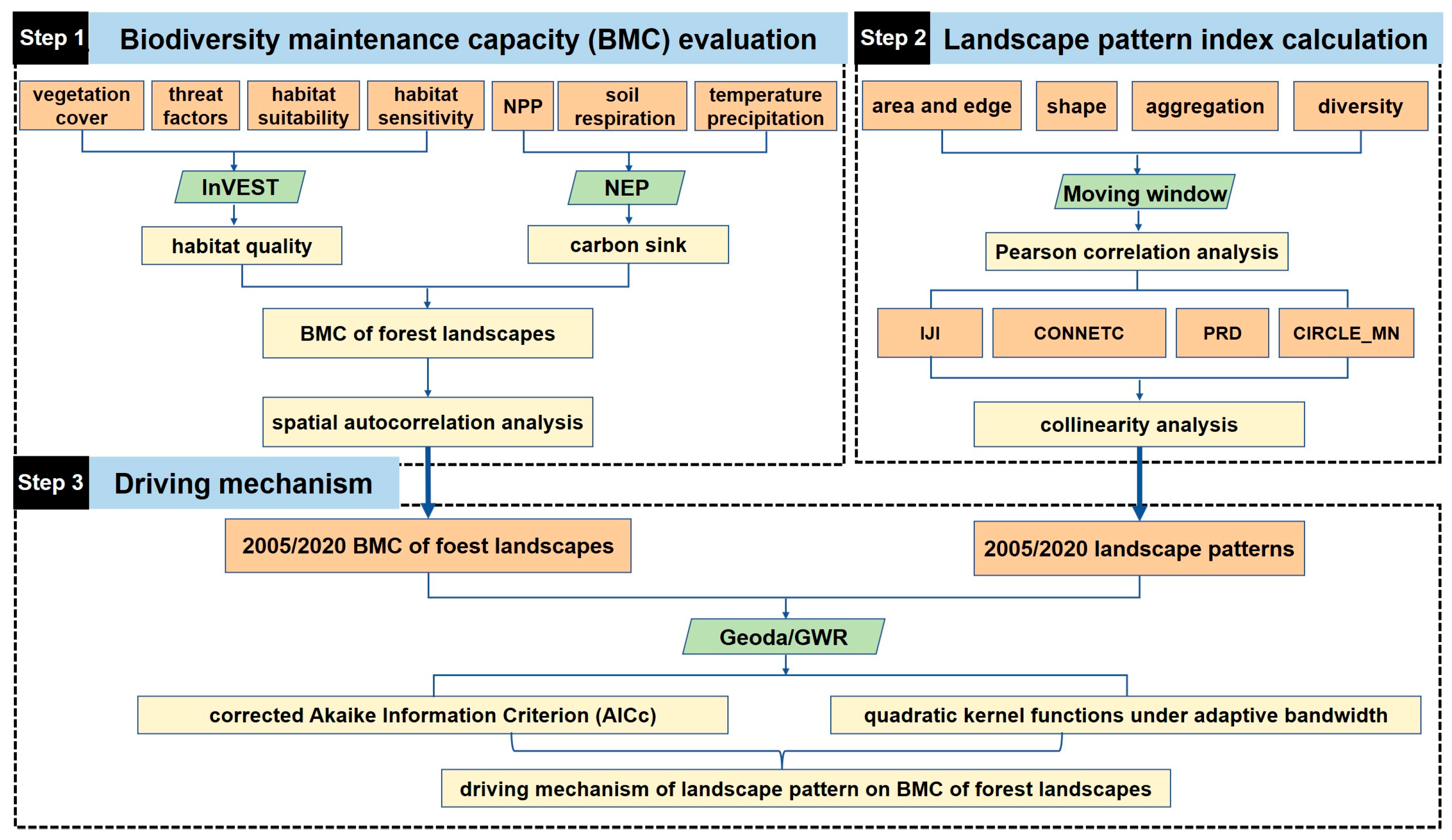
Figure 1. Working flow chart of this study. Note: Landscape indices include: IJI, intermixing and juxtaposition index; CONNECT, connectance index; PRD, patch richness density; CIRCLE_MN, mean of the related circumscribing circle. See the supporting document (Table S2) for landscape indices descriptions.
Land 12 01293 g001
Figure 2. Geographic location of Beijing, China. (a) A map displaying the elevation of the study area, with an inset showing the location within China. (b) A map displaying the administrative districts of Beijing, along with the distribution of forest landscapes. (c) A map depicting the urban, suburban, and mountain areas.
Land 12 01293 g002
Figure 3. Land use maps for Beijing during (a) 2005 and (b) 2020.
Land 12 01293 g003
Figure 4. Spatial distribution of different BMC classes of forest landscapes in Beijing in (a) 2005 and (b) 2020; (c) alteration in the spatial pattern of BMC between 2005 and 2020. Note: significant degradation or improvement means the BMC of forest landscapes underwent dramatic changes across multiple classes from 2005 to 2020; stable means the BMC of forest landscapes remained at the same class from 2005 to 2020; slight degradation or improvement means the BMC of forest landscapes varied between consecutive classes.
Land 12 01293 g004
Figure 5. Evaluation results of the four landscape pattern indices (IJI, CONNECT, PRD and CIRCLE_MN) in 2005 and 2020. Note: The black lines in (ac,e) represent the boundaries between the urban center region, suburban region, and mountainous region. The white lines in (d,fh) also represent the same boundaries.
Land 12 01293 g005
Figure 6. Moran scatter plots of biodiversity maintenance capacity (BMC) values in (a) 2005 and (b) 2020.
Land 12 01293 g006
Figure 7. Results of local spatial autocorrelation analysis of the biodiversity maintenance capacity of forest landscapes at the street and township administrative scales: LISA agglomeration maps in (a) 2005 and (b) 2020; local Moran’s I significance maps in (c) 2005 and (d) 2020. Note: High-High (H-H) means high-value districts adjacent to neighboring high-value districts; Low-Low (L-L) means low-value districts adjacent to neighboring low-value districts; High-Low (H-L) means high-value districts adjacent to neighboring low-value districts; Low-High (L-H) means low-value districts adjacent to neighboring high-value districts. Note: Black lines represent the boundaries between the urban center region, suburban region, and mountainous region.
Land 12 01293 g007
Figure 8. Average geographic weighted regression coefficients of the four landscape pattern indices (IJI, CONNECT, PRD, and CIRCLE_MN) in 2005 and 2020. Note: The white lines in (a,b,h) represent the boundaries between the urban center region, suburban region, and mountainous region. The black lines in (cg) also represent the same boundaries.
Land 12 01293 g008
Table 1. Threat factors and their corresponding coefficients considered in the InVEST model. Note: drmax, maximum effect distance (km); wr represents the effective weighting of each threat factor; Sensitivity refers to the degree of impact or responsiveness of forest landscapes to each threat.
Threat FactordrmaxwrDistance–Decay FunctionSensitivity
Cultivated land80.68Linear0.7
Urbanized land101Exponential0.8
Railway90.9Exponential0.55
Primary road81Linear0.85
Secondary road50.75Linear0.77
Table 2. Comparative analysis of model fitting results for 2005 and 2020 using the Ordinary Least Squares (OLS) and Geographic Weighted Regression (GWR) models. Note: AICc, Akaike Information Criterion.
Parameter20052020
OLSGWROLSGWR
Adjusted R20.540.680.830.86
AICc−865.64−817.07−915.12−884.12
Table 3. Land use transition matrix for Beijing between 2005 and 2020. (Unit: km2).
2020GrasslandCultivated LandUrbanized LandForest LandWater AreaUnused LandTotal
2005
Grassland-66.8729.33712.328.1236.55853.18
Cultivated land432.94-819.831956.1621.16333.763563.85
Urbanized land56.81252.51-343.7715.8099.66768.55
Forest land1108.4558.3943.61-5.9739.481255.90
Water area30.24104.8537.5993.77-46.25312.68
Unused land0.330.100.100.260.16-0.95
Total1628.77482.71930.463106.2751.21555.696755.11
Table 4. Area and proportion of forest landscapes with five classes of BMC in 2005 and 2020 (units: area, km2; ratio, %).
BMC Class20052020
AreaRatioAreaRatio
I0.210.01%1324.0316.86%
II210.713.54%118.441.51%
III2796.1546.95%97.031.24%
IV2834.2747.59%2217.0328.23%
V113.801.90%4097.6452.17%
Table 5. Transfer matrix between different BMC classes of forest landscapes in Beijing from 2005 to 2020. (Unit: km2).
2020IIIIIIIVVTotal
2005
I0.020.000.010.010.000.04
II14.851.722.4867.2344.13130.40
III104.9915.0111.60865.99989.581987.17
IV34.5410.625.18426.691943.422420.45
V1.230.030.040.99110.22112.51
Total155.6327.3819.301360.903087.364650.57
Table 6. Results of geographic weighted regression (GWR) results of landscape indices and biodiversity maintenance capacity of forest landscapes.
Landscape IndexAverage ValueMinimum ValueMedianMaximum Value
20052020200520202005202020052020
IJI0.0020.003−0.007−0.0110.0020.0010.0170.017
CONNECT−0.001−0.003−0.011−0.0240.0000.0000.0150.014
CIRCLE_MN−0.3211.130−3.042−1.287−0.0691.1513.8022.806
PRD0.007−0.009−0.040−0.0600.005−0.0030.1570.038
Disclaimer/Publisher’s Note: The statements, opinions and data contained in all publications are solely those of the individual author(s) and contributor(s) and not of MDPI and/or the editor(s). MDPI and/or the editor(s) disclaim responsibility for any injury to people or property resulting from any ideas, methods, instructions or products referred to in the content.