Matching Relationship between Urban Service Industry Land Expansion and Economy Growth in China

Abstract

In the era of the urban economy and service economy, the decoupling of service industry land expansion from economic growth has always been a key measure to evaluate sustainable and healthy development. Based on the decoupling model and GIS spatial analysis method, this paper conducted an empirical study of Chinese cities from 2012 to 2019. Results: (1) Increasing spatial heterogeneity, correlation and agglomeration of land expansion were found in China’s urban service industry and its economic growth; (2) Most cities were in weak decoupling, with evolved, degraded and unchanged cities accounting for one-third each, and the number of cities in negative decoupling was increasing, leading to increasingly diverse and complex decoupling relationships; (3) From the perspective of changes in the urban service industry land and its decoupling from economic growth, HH cities were clustered in the Yangtze River Delta, Pearl River Delta, Beijing–Tianjin–Hebei and Chengdu–Chongqing urban agglomerations in a continuous belt pattern, while LL and HL cities were mostly in the north, especially in the northeast, creating many cluster-like agglomerations that have become problematic spaces; (4) A significant synergistic effect was identified between the factors of urban permanent population, value added of the secondary industry, per capita GDP, government financial expenditure, international trade, foreign direct investment, total retail of commodities, and authorized patents, with factor pairs formed showing nonlinear enhancement. The factor value added of the secondary industry had the largest direct impact, while urban permanent population and foreign direct investment led in terms of net synergies; (5) It is recommended to introduce classified and differentiated urban service industry land use policies, plan and build a number of national, provincial and municipal modern service industry clusters, demonstrate changes in land supply and use, build a scientific and efficient land resource allocation and management system, guard against and prevent recoupling and effectively improve the ability of cities to achieve high-quality economic development.

1. Introduction

1.1. Background

Today the service industry is playing an increasingly important role in the industrial revolution and economic development, and more and more countries are transitioning their economic systems from industrial to service-oriented systems [1,2]. According to World Bank data, the proportion of the service industry in the GDP of developed countries such as the United States, Britain, France, Canada, Singapore, Israel and Japan reaches or exceeds 70%, and it is more than 50% even in developing countries such as China, Egypt, India, Iran, Turkey, Malaysia, Thailand, Brazil and Russia [3]. The transformation of industrial structure drives and influences the change of urban land use, and the study of the change of urban service land use and its relationship with economic development has become an important topic in economic geography and spatial planning [4,5].

According to the National Bureau of Statistics of China, the added value of China’s service industry was USD 8031.69 billion in 2020, a huge scale that makes China a major service economy in the world. In 2012, China’s service industry output exceeded 50% of the GDP and has now reached 54.5%, making China a typical service-oriented economy. Cities are the central engine of local and regional construction in China, and the structure, scale and efficiency of their land use is changing dramatically as more and more industrial cities are transformed into service-oriented ones. Urban economies are becoming service-oriented, a fact that inevitably drives adaptive changes in urban land planning, supply and management tools [6,7]. However, blocking the coupling between economic growth and resource consumption and environmental pollution and decoupling economic growth from environmental resources are the key to achieving high-quality development [8]. Due to the huge land use and economic scale of China’s urban service industry, exploring the relationship between land expansion and economic growth in China’s urban service industry and identifying whether service economy growth depends on expanded land use or land consumption in the process of urban development are not only of great importance for the sustainable and healthy development of Chinese cities, but also provide typical cases for other countries in the world [9,10].

1.2. Literature Review

1.2.1. Service Industry Land Use

Now more and more scholars are focusing on service industry land use, and the analysis of the impact of changes in transportation modes such as subways, high-speed railways and viaducts on changes in service industry land use, such as supply patterns, utilization patterns and socio-economic benefits, has become a central research topic in the field. Wang [11], Shao [12] and Tian [13] et al. concluded, based on case studies in the lower reaches of the Yangtze River and the Wuhan–Guangzhou high-speed railway region, that there is still a great deal of uncertainty as to whether the construction of high-speed rail stations and the increased frequency of a train service will drive the development of the service sector. Tian [14] and Yang [15] found that high-speed rail has a significant effect on the spatial agglomeration of urban service industries and is closely related to the location of stations in the high-speed rail network, based on multiple measurements of Chinese urban panel data over many years. Sheng [16] conducted an evaluation of the economic benefits of Grey Space based on the case study of Wuhan.

Analyzing service industry land uses and their changing impacts on the surrounding environment has become a popular topic, including impacts on adjacent land use patterns and asset values, urban community security environments and criminal behavior, spatial accessibility and economic development. Yang concluded that service industry land has positive and negative externalities on residential land, with the economic benefits of residential land increasing and then decreasing as service industry land becomes more concentrated [17]. Sohn and Browning concluded that the change of the composite pattern of service industry land will have a completely different impact on the security environment of the community [18,19]. Service industry land use forms such as catering, business, office and retail can improve the security of the residential environment. Commercial and residential densities are positively correlated with criminal activity. Izanloo believes that service industry land use is positively correlated with traffic behavior and has a strong impact on spatial accessibility [20]. Langer found that the increase in commercial land area has led to a significant increase in tax revenues in Bavarian cities, but there are great differences between cities [21]. In addition, the study of commercial land price changes and their influencing factors has also received some scholarly attention. Nichols [22] studied the commercial land price fluctuations in America; Garang [23] studied the spatiotemporal change mechanisms of service land prices and concluded that factors such as the price level of residential land, the maturity of living services and the plot ratio have a strong influence on commercial land prices. Ustaoglu [24] and Silva [25] analyzed the factors driving the change in demand for service industry land.

To sum up, the studies on service industry land have aroused the concern of the government and scholars. However, there is much to be desired. First of all, in most cases these studies focus on the case of a particular city while ignoring the overall study of most or even all cities in a given country, resulting in no systematic understanding of service industry land use and its changing patterns. Secondly, the papers available mainly focus on the demand for service industry land, development patterns, land price changes and their interaction with the surrounding community environment, but there is no research on the relationship between service land efficiency, land supply and service economy demand, making them not sufficiently supportive for policy design.

1.2.2. Decoupling of Economic Growth

The decoupling model mainly applies to economic and human geography, landscape and ecology, resource utilization and environmental protection. This paper presents an analysis of the match between economic output and resources [26,27], energy [28,29,30] input or consumption, ecological footprint [31], haze [32,33], harmful and greenhouse gas emissions (such as sulfur dioxide [34], carbon [35,36], ammonia [37] and nitrogen oxides [38]), environmental pollution [39], waste generation [40] and the development trend. In recent years, more and more scholars have begun to study the match between land change and economic and population growth, with focus on the coordination between land productivity, construction land growth and economic development, population growth, greenhouse gas emissions and the scale of concentration of migrant workers [41,42].

In the field of land use change and high-quality economic development, the application of decoupling models for coupling analysis has become a hot topic. For example, Shao argued, based on the Tapio decoupling model, that the land use intensification and heat island effect in Shijiazhuang were negatively decoupled from 1995 to 2004 and their relationship shifted to weak decoupling from 2004 to 2016 [43]. Li found a weak decoupling relationship between carbon emissions generated from construction land and the economic benefits created, with energy intensity being an important influencing factor [44]. According to Li, the change in population size and the growth of urban and rural construction land in Hebei are generally not coordinated, mainly manifesting as weak decoupling [45]. Hubei Province, however, is very different, with only a few counties in a coordinated state [46]. Liu classifies the coordination relationship between urban construction land expansion and changes in the number of migrant workers into eight types [47]. Wang found a negative decoupling between population and construction land in most counties in Hubei Province, and only nine are in a coordinated state.

Existing papers generally focus on the compound relationship between land and economic growth, usually analyzing construction land as an overall variable in relation to economic growth, population change and pollutant emissions but with no attention to specialized studies on subdivided land types. Apart from some exploratory studies by Guo, there are no other studies on the relationship between one or more types of land use and economic development [48]. Construction land contains residential land, industrial land, service industry land, administrative land, logistics land, transportation land, utility land, green land and land of many other types, and the different land types maintain widely varying relationships with economic development. Therefore, in the context of the transformation of the urban economy from the industrial era to the service era, it is of great theoretical significance and practical value to conduct research on the relationship between service industry land use change and economic growth based on the decoupling model and reveal the evolution pattern and development trend of the relationship to provide a basis for decision making on service industry land use management and service economy development.

1.3. Aim and Question

The dramatic expansion of demand for service industry land in the urban economy during the transition from industrial cities to service-oriented cities has made the service economy an important part in determining the level and capacity of sustainable urban development [49]. To accurately identify the complex relationship between land expansion in the service industry and economic growth, we conducted an empirical study of China from 2012 to 2019 by GIS spatial analysis using a decoupling model. This paper aims to address the following questions: What are the patterns of land use change in urban services in the temporal and spatial dimensions? What are the driving factors for the expansion of service industry land? What is the decoupling relationship between urban service industry land expansion and economic growth? What are the characteristics or trends of decoupling relationship changes, and how should they be dealt with in policy design? Answering the above questions will help reveal the characteristics of service land changes in cities in different periods and their correlation with economic growth and provide a reference for decision making on policy design for service land supply and economic development.

2. Research Design

2.1. Study Area: China

This study is conducted on 273 prefecture-level and above cities in China, accounting for 92% of all those in similar conditions in China, covering most provinces, cities and municipalities directly under the central government, including Jiangsu, Zhejiang, Anhui, Henan, Shaanxi, Gansu, Guangxi, Guangdong, Heilongjiang, Liaoning, Beijing, Shanghai, Tianjin and Chongqing (Figure 1).

For the sake of spatial integrity and coherence, as well as data accessibility and comparability, this study does not cover those cities in the Hainan, Yunnan, Tibet, Xinjiang and Qinghai provinces, besides autonomous prefectures, provincial counties and county-level cities in Sichuan, Gansu, Guizhou, Inner Mongolia, Heilongjiang and Hubei, due to three considerations as follows. Firstly, the distribution pattern of western provinces and ethnic autonomous regions with mainly autonomous prefectures and counties and only a small number of prefecture-level cities would make their inclusion in the study area likely to bring many isolated prefecture-level cities, thus hindering spatial association analysis. For example, Qinghai has only two cities, Xining and Haidong, and Xinjiang has only four cities, Urumqi, Karamay, Turpan and Hami, which would be isolated points if they were included in the study area. In addition, many of the prefecture-level cities in these regions are newly established ones, and they do not have sufficient historical data to support a sufficient and extensive analysis. Secondly, data on the development of the autonomous prefectures are scarce and hard to collect due to the difference in statistical systems, policies and standards. Thirdly, Tianmen, Xiantao, Qianjiang and other provincial counties or county-level and prefecture-level cities are not at the same administrative level or level of development capacity, making it inappropriate to place them together for comparative analysis.

2.2. Technical Roadmap and Research Methods

2.2.1. Research Steps

Three research steps are included in this paper (Figure 2).

The first step is the data preprocessing. It involves collecting and collating data on all indicators of 273 cities from 2012 to 2019 released by the Chinese government’s statistics department. The second step is the result analysis. We first study the spatial characteristics of urban service industry land change by GIS cluster analysis and spatial autocorrelation analysis (calculated as shown in Section 2.2.2). Next, we analyze the relationship between service industry land use change and economic growth from three dimensions of the service industry, urban economy and government revenue (calculated as shown in Section 2.2.3). Then we compare and analyze the results of the first two in different time periods, trying to extract the trend of development and change, while analyzing the impact mechanism of different factors on the decoupling effect (calculated as shown in Section 2.2.4) based on GeoDetector. The third step is the discussion and application of the results. We discuss the findings and limitations of this paper in terms of development trends and spatial characteristics, and further attempt to propose targeted solutions and improvement suggestions for city governments in their policy design.

2.2.2. Exploratory Spatial Data Analysis and Spatial Clustering Analysis

ESDA is a “data-driven” analysis method that uses spatial autocorrelation as a statistical indicator to measure the level of spatial interdependence of variables. Spatial interdependence includes global spatial autocorrelation and local spatial autocorrelation. Both Global Moran’s I and Local Moran’s I are the two principal spatial autocorrelation coefficients of ESDA (see Zhang et al. [50] for their equations), with the former exploring the spatial distribution and correlation characteristics of observations across the region, while the latter focuses on the spatial distribution patterns and spatial heterogeneity of observations in sub-regions. It should be noted that the Moran’s I value ranges from −1 to 1, and a value greater than zero, less than zero or equal to zero represents positive, negative autocorrelation and random distribution, respectively. Clustering analysis is a mathematical method for classifying objects in a spatial data set into different types or sets based on how similar and close their attributes or variables are to each other. Spatial clustering analysis is an unsupervised learning method that does not require a priori knowledge. Algorithms such as quantile, natural break, K-means and K-medoids are allowed in the process of cluster analysis. In this paper, the quantile algorithm is used to classify urban service land and economic-related indicators into high, medium and low levels. Spatial autocorrelation analysis is used to measure the effect of spatial association based on Goodhild‘s Second Law of Geography, while spatial clustering analysis is used to measure the effect of spatial differentiation based on Goodhild‘s Second Law of Geography [51].

2.2.3. Decoupling Model

Originating in physics, decoupling theory was pioneered by the Organization for Economic Cooperation and Development (OECD) for use in economics and has now become a well-established quantitative method for analyzing the relationship between economic growth and resource consumption and environmental change. The OECD defines decoupling as the breakdown of the coupling between economic growth and environmental shocks, i.e., the absence of simultaneous changes between the two. The OECD proposes a method for calculating decoupling indicators and further classifies the types of decoupling into absolute, relative and non-decoupling [52]. The decoupling theory proposed by the OECD has obvious shortcomings, specifically, the different choices of the base period cause changes in the decoupling index, which leads to uncertainty in the determination of the decoupling type; moreover, the fewer delineations of the decoupling types lead to rougher conclusions of the study, which is of low guiding significance for practical application [53,54]. The current common decoupling model is the one proposed by Tapio, which is adopted in this paper. The Tapio decoupling model uses the elasticity coefficient method to calculate decoupling indicators, with 0.8 and 1.2 as the thresholds for decoupling indicator classification and classifies decoupling types into 8 categories according to the direction (positive or negative) of economic output and resource consumption growth [55]. The Tapio decoupling model cleverly sidesteps the shortcomings of the OECD model and it has been used as a primary tool to measure the compatibility of urban economic growth with resource consumption and environmental change and the possibility to achieve sustainable development [56,57].

This paper analyzes the relationship between urban service industry land and economic growth using the Tapio decoupling model to reveal whether there is a correlation between the two with synchronous or asynchronous changes. Value added of service industry is the direct output brought by the service industry land, and the analysis of the decoupling relationship between service industry land and value added is the most direct indicator to determine the intensification of service industry land use. Moreover, the service industry stimulates and interacts with industrial development and has a non-negligible effect on the overall development of urban economy [58,59]. Therefore, this paper analyzes the decoupling relationship between service industry land and GDP of municipal districts and tries to reveal the relationship between service industry land and high-quality development of the urban economy. In addition, income generation is a powerful driving force for the government to promote industrial development, and fiscal revenue is a common indicator of comprehensive government revenue. In the context of relying on land finance, changes in the supply of land for service industries have a significant impact on the fiscal revenue of city governments. Against the background of increasingly tight land resources, the analysis conducted in this paper on the decoupling relationship between service industry land and fiscal revenue helps provide a basis for city governments to optimize the scale and structure of land supply.

The decoupling indicator between service industry land and economic growth is calculated by the following equation, where $\epsilon$ represents the decoupling indicator, $\Delta \alpha$ represents the average annual growth of service industry land, ${SL}_i$ and ${SL}_{i+n}$ represent the values of service industry land area in years $i$ and $i+n$, respectively, $\Delta \beta$ represents the average annual growth of economic output indicators (including value added of service industry, GDP and fiscal revenue), ${OP}_i$ and ${OP}_{i+n}$ represent the annual values of economic output indicators in years $i$ and $i+n$, respectively, and $n$ represents the study time period:

$$\epsilon =\frac{\Delta \alpha }{\Delta \beta }, \Delta \alpha =\sqrt[n]{\frac{{SL}_{i+n}}{{SL}_i}}, \Delta \beta =\sqrt[n]{\frac{{OP}_{i+n}}{{OP}_i}}$$

(1)

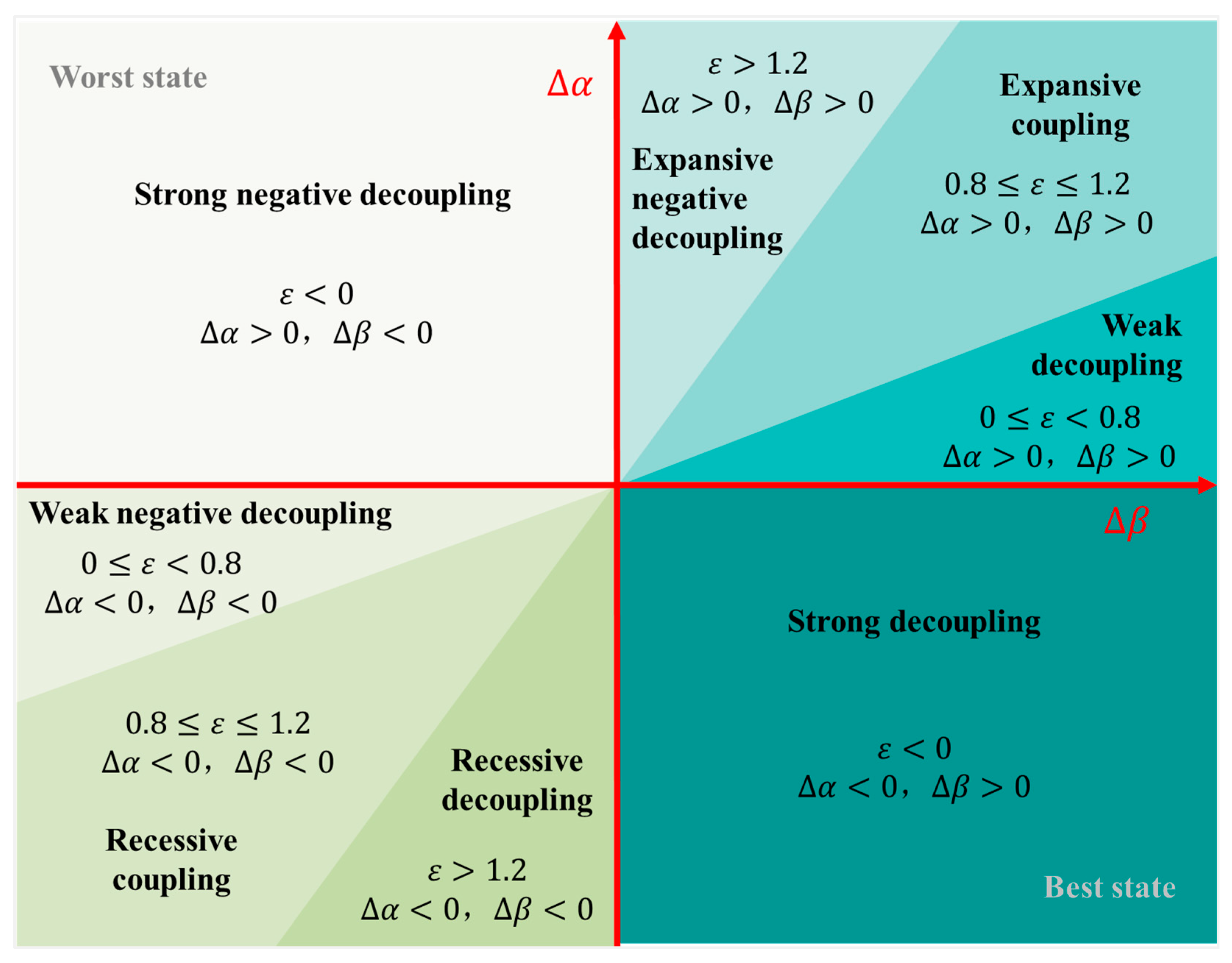
Based on the experience from relevant research [60,61], and the positive and negative results of $\Delta \alpha$ and $\Delta \beta$, this paper classifies the decoupling into 3 types and 8 sub-types with 0.8 and 1.2 as the classification thresholds for $\epsilon$ (Figure 3). The first type is decoupling, including three sub-types of strong decoupling, weak decoupling and recessive decoupling. Strong decoupling is the most favorable state, which implies continued growth in economic output while the size of service land continues to shrink, indicating a highly intensive use of service industry land. Weak decoupling ranks second, which shows that the economic output index grows rapidly along with the expansion of service industry land, with the economic growth faster than the land growth, indicating an efficient use of service industry land. Recessive decoupling is unfavorable, which shows that the service industry land use and economic output are shrinking, with land use declining at a faster rate, indicating an intensive land use contraction. The second type is coupling, including two sub-types of expansive coupling and recessive coupling. It reflects the simultaneous rise or fall in service industry land with the change of economic output, standing for an intermediate transitional state between intensive and extensive land use. The third type is negative decoupling, including three sub-types of strong, weak and expansive negative decoupling, and all indicating unhealthy states of extensive land use. Strong negative decoupling is the most unfavorable, showing that the corresponding economic output keeps declining in the face of the growth of service industry land. Weak negative decoupling shows a decrease in both the size of service industry land and economic output, with a faster economic downturn. Expansive negative decoupling shows that both service industry land and economic output are growing, with the land consumption at a higher speed.

The concept of “decoupling” emphasizes the trend of decoupling, that is, it emphasizes that the decoupling relationship between land resource consumption and service economy, GDP and fiscal revenue growth is not a short-term process, but a process of adjustment that requires a certain period and cost. There is a time lag from site input to output, so a lead time is required for construction and development. Additionally, the analysis of economic and social development should maintain overall policy consistency as much as possible, because both the central and local governments in China implement a “five-year planning” system for urban economic development to ensure a relatively stable policy environment over a five-year period. Accordingly, based on the five-year plan and the time series of available data, this paper uses n = 4 and controls time periods in the 12th Five-Year Plan (2012–2015) and the 13th Five-Year Plan (2016–2019).

2.2.4. GeoDetector

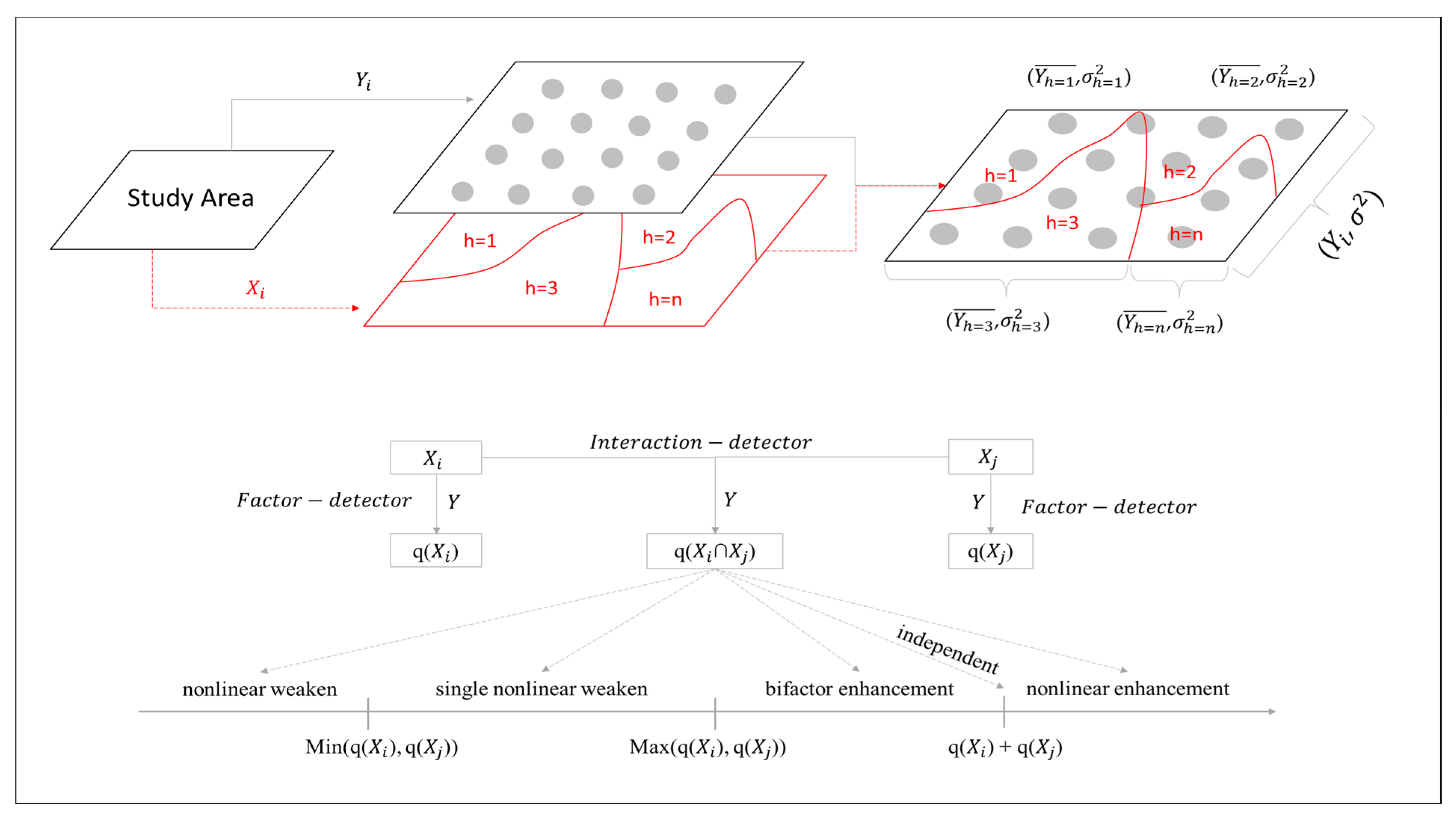
GeoDetector is a free and open software application, available at http://geodetector.cn/ (13 August 2021). The decoupling between urban service land expansion and economic growth reveals significant spatial effects, and the driving mechanism cannot be analyzed directly by the traditional statistical regression models (OLS) or other methods. GeoDetector takes full account of the spatial effects in its analysis and explains the driving forces behind geographic phenomena by detecting the similarity between spatial patterns of independent and dependent variables (Figure 4). As an emerging spatial econometric model, it is now widely used to study the natural and socio-economic influences.

GeoDetector calculates and outputs $q$ index, ranging from 0 to 1, with larger values indicating greater impact. In this paper, factor detection and interaction detection modules of GeoDetector are borrowed to analyze the direct and indirect influences of different factors on decoupling. In the direct impact analysis, the $q$ index represents the direct driving force of different factors (e.g., $X_i$ and $X_j$) on decoupling, expressed by q($X_i$) and q($X_j$)). In the indirect impact analysis, the $q$ index represents the interactive driving force on decoupling when factors $i$ and $j$ interact with each other, expressed by q($X_i$∩$X_j$). According to the relationship of q($X_i$∩$X_j$)) with the minimum (Min(q($X_i$), q($X_j$))), maximum (Max(q($X_i$))), q($X_j$))) and sum (q($X_i$) + q($X_j$)) of the direct driving forces, the interaction influence is classified into five types, and the relevant measures and recommendations can be combined or matched according to the interaction between factors in the policy design stage [62]. The equation for $q$ is as follows [63], where h is the number of zonings of the influencing factor in the study area (2–10 in this paper), $N_h$ and N are the numbers of cities in zoning h and the study area, ${\sigma }_h^2$ and ${\sigma }^2$ are the squares of the decoupling effect in zoning h and the study area, SSW is the sum of squares within the zoning (Within Sum of Squares) and SST is the number of total squares in the study area (Total Sum of Squares):

$$q=1-\frac{\sum _{h=1}^l{N}_h{\sigma }_h^2}{N{\sigma }^2}=1-\frac{SSW}{SST}$$

(2)

$$SSW=\sum _{h=1}^l{N}_h{\sigma }_h^2$$

(3)

$$SST=N{\sigma }^2$$

(4)

The development of the service economy is affected by population, industrialization, government investment, international trade, social policy environment and other factors, which is the fundamental reason for the change in urban service land. The service industry is usually classified into production- and consumer-oriented service industries. The size of regional population and urbanization level are major factors affecting the development of consumer-oriented services, and it is represented by the urban permanent population; in the general trend of promoting the integrated development of manufacturing and service industries, industrialization is a major factor affecting the development of production-oriented services, and it is represented by the secondary industry and per capita GDP in this paper. The government has given great support that can never be ignored in China’s transition from a manufacturing economy to a service economy, for example, the central government has promulgated policies such as Guidelines for Accelerating the Development of High Technology Service Industry, Several Opinions on Promoting the Development of Health Service Industry and Measures for the Management of Funds for the Development of Service Industry, with increased investment in the service industry. In this paper, it is represented by government financial expenditure. In addition, service trade is positioned as an important area of China’s opening up and cooperation, and the central government has designated Tianjin, Shanghai, Hainan, Chongqing, Shenyang, Nanjing, Hangzhou, Wuhan, Guangzhou and Chengdu as national pilot sites for the expansion and opening up of the service industry. Therefore, globalization also has a great influence on the development of the service economy, and we use international trade and foreign direct investment to represent it. With the increasingly intense trade war and science and technology war between China and the United States in recent years, China has launched a new domestic and international dual-cycle development strategy, attaching great importance to expanding domestic demand and stimulating the power of independent innovation. It has released the Outline of Strategic Planning for Expanding Domestic Demand (2022–2035), which focuses on science and technology as the first productive force, talents as the first resource and innovation as the first driving force, while seeking to deeply implement the strategy of developing the country through science and education, the strategy of relying on talents to strengthen the country and the strategy of adhering to innovation to drive development. Therefore, the consumption and innovation orientation of China’s macroeconomic and social development will also have an impact on the development of the service economy, which is represented in this paper by total retail sales of goods and granted patents.

2.2.5. Data Sources

In this paper, the term “service industry” is equivalent to the tertiary industry, but the two are different only in usage habits. Statistically, the term “tertiary industry” is used when it is juxtaposed with primary and secondary industries, while the term “service industry” is often used when it is juxtaposed with “agriculture, forestry, animal husbandry and fisheries” and “industry and construction”. The urban service land in this paper, or “Class B land” in the Code for Classification of Urban Land Use and Planning Standards of Development Land, includes commercial land; retail approval land; catering and accommodation land; financial and insurance land; cultural and creative land; entertainment and leisure land; health, science and technology service land; and engineering consultation and technical service land. The year 2012 was chosen as the base period for the study because, on the one hand, China began to release land use statistics for urban service industries with a stable and consistent caliber in 2012, and on the other hand, the service industry became the top sector in China in 2012, marking the transformation of China as a whole from an industrial economy to a service economy.

The data used in the research process mainly came from the China City, Construction, and Tertiary Industry Statistical Yearbook published by the NBSC (National Bureau of Statistics of China, Beijing, China) and MHURDC (Ministry of Housing and Urban-Rural Development of China, Beijing, China) from 2013 to 2020. If the data were missing, mathematical methods were used for interpolation estimation. In case of missing data for the first and last years or missing data for consecutive years, such as the data of Jilin and Baishan in 2019, estimates were made by trend extrapolation based on the data of the same policy area. For the data accidentally missing in a certain year, such as data of Zunyi and Jiamusi in 2018, Chongqing in 2017, and Jinzhou in 2016, estimates were made by the mean value method based on the data of the adjacent years before and after.

3. Results

3.1. Dynamic Analysis

3.1.1. Spatial Heterogeneity

Shanghai had the Max service industry land area of 135.21 km² and 137.54 km² in 2012 and 2015; while Beijing took its place with the Max of 135.13 km² and 137.98 km² in 2016 and 2019, respectively. Qitaihe had the Min service industry land area of 0.08 km² in 2012; the Min was found in Qingyang and Dingxi in 2015 and 2016, decreasing to 0.02 km² and 0.03 km²; in 2019, Qingyang and Longnan had the Min, elevating to 0.04 km². In general, the SUM and Average of service industry land in the study area increased over the years, with the Max and Min in dynamic change and both land expansion and contraction in coexistence. The Max service industry added value remained in Shanghai, while the Min remained in Heihe, along with gross domestic product. The Max, Min, Average and SUM of service industry added value and gross domestic product were in positive growth. Shanghai remained the city to have the Max service industry land, which was USD 86.57 billion, USD 59.51 billion, USD 96.44 billion and USD 103.86 billion, respectively, experiencing a change process of growth followed by decrease; the Min was found in Hechi, Guyuan and Ya’an, respectively, which, like Average and SUM, experienced a change process of decrease followed by growth (

Table 1. Statistical analysis of urban service industry land and economy.

Year	Indicator	Max	Min	Average	Sum
2012	Service Industry Land	135.21	0.08	9.40	2566.06
	Service Industry Added Value	214.51	0.17	8.99	2455.51
	Gross Domestic Product	315.97	0.41	18.51	5052.91
	Government Revenue	58.72	0.03	1.97	536.73
2015	Service Industry Land	137.54	0.02	10.13	2766.83
	Service Industry Added Value	294.32	0.20	13.04	3559.61
	Gross Domestic Product	398.79	0.48	24.55	6700.85
	Government Revenue	87.74	0.04	2.87	782.23
2016	Service Industry Land	135.13	0.03	10.59	2890.18
	Service Industry Added Value	310.05	0.33	13.79	3765.80
	Gross Domestic Product	424.23	0.51	25.13	6860.40
	Government Revenue	96.44	0.05	2.88	786.72
2019	Service Industry Land	137.98	0.04	11.90	3247.59
	Service Industry Added Value	428.24	0.39	18.49	5046.58
	Gross Domestic Product	553.11	0.55	31.08	8484.89
	Government Revenue	103.86	0.03	3.19	870.38

Note: The unit of land area is square kilometers, and the other indicators are in billions of US Dollars. The average exchange rates between the Chinese Yuan and the US dollar in 2012, 2015, 2016 and 2019 were 6.3124, 6.2284, 6.6423 and 6.89852, respectively.

).

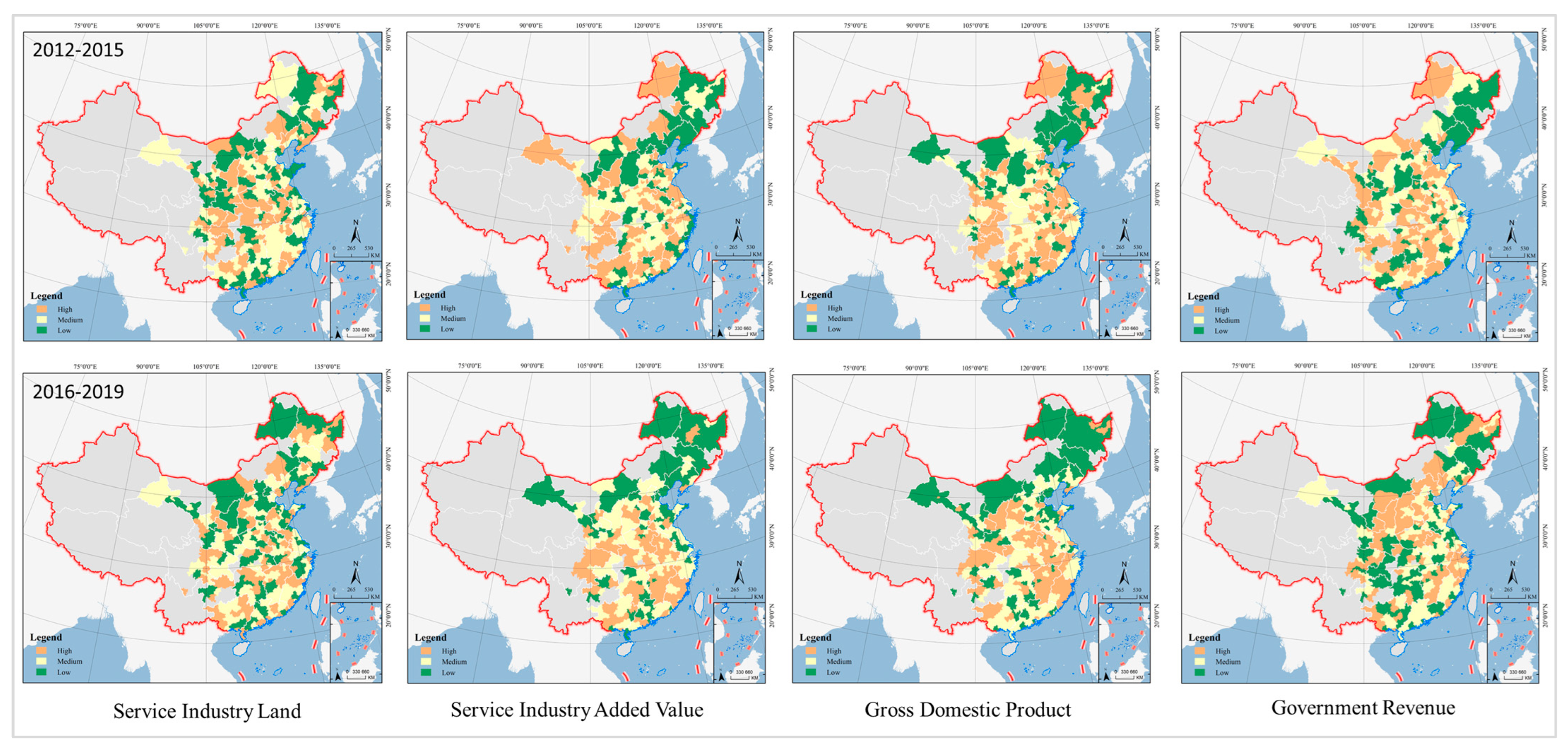
The spatial heterogeneity and agglomeration of urban service industry land use and its economic growth in China are significant and increasing (

Table 2. Statistical analysis of average annual growth rate.

		Max	Min	Average	Coefficient of Variation	Global Moran I
2012–2015	Service Industry Land	208.55	−81.42	10.61	3.08	−0.03 (0.111)
	Service Industry Added Value	61.38	−12.93	13.59	0.58	0.15 (0.001)
	Gross Domestic Product	80.87	−20.27	9.07	1.12	0.20 (0.001)
	Government Revenue	74.77	−30.15	12.81	1.17	0.22 (0.001)
2016–2019	Service Industry Land	431.38	−41.91	8.04	3.83	−0.22 (0.427)
	Service Industry Added Value	189.60	−23.49	13.35	1.08	0.16 (0.001)
	Gross Domestic Product	189.22	−25.15	8.87	1.60	0.09 (0.002)
	Government Revenue	68.15	−44.32	4.44	2.90	0.07 (0.002)

Note: Significance values are in parentheses, and the Global Moran’s I index is statistically significant when p ≤ 0.1.

). The studies of Guan [64], Liu [65], Miyamoto [66] and She [67] show that a coefficient of variation greater than 0.36 leads to highly discrete and unbalanced variables. The coefficients of variation of service industry land, government revenue, gross domestic product and service industry added value were all much greater than 0.36 and they were increasing from 2012–2015 to 2016–2019. This paper conducts a spatial clustering analysis by the quantile method of ARCGIS and classifies the urban service industry land and its economic growth in China into three types of high, medium and low levels. Changes in urban service industry land use in China show that high-growth cities are becoming increasingly geographically dispersed, while those with low growth are increasingly clustered in the northeast and northwest. From the perspective of economic development changes, cities with high-growth and low-growth service industry added value, gross domestic product and government revenue are increasingly concentrated, mainly showing a cluster-like agglomeration with great variation in spatial pattern. It should be noted that long-term lagging development has made northeastern and northwestern cities a problematic region affecting China’s coordinated regional development.

From the perspective of changes in service industry land, the maximum annual growth rate was further expanding from 2012 to 2015 and from 2016 to 2019, while the minimum and average values were decreasing. From 2012 to 2015, the high-level cities were mainly distributed in Chongqing, Henan and Hubei; the medium-level cities gathered in Jiangxi, Fujian, Zhejiang, Hebei and Shaanxi; and the low-level cities were clustered in Jilin, Heilongjiang, Gansu, Ningxia, Shaanxi and Inner Mongolia. The cities of high and medium levels in 2016 to 2019 were more dispersed, with the former distributed in small agglomerations only in Anhui and Zhejiang, and the latter only in Zhejiang and Fujian. Lower-level cities were becoming more geographically concentrated, mainly in Heilongjiang, Liaoning, Hebei, Inner Mongolia, Shaanxi, Gansu, Ningxia and other northeast and northwest regions (Figure 5).

From the perspective of the service industry added value, the maximum and minimum annual growth rates were further expanding in 2012–2015 and 2016–2019, and the average remained relatively stable. The cities of a high level in 2012–2015 were mainly distributed in Guangdong, Guizhou and Fujian; the cities of a medium level gathered in Sichuan, Shaanxi, Henan and Hunan; and the cities of a low level were clustered in Liaoning, Jilin, Heilongjiang, Hebei, Shanxi and Inner Mongolia. The cities of high and low levels were more concentrated from 2016 to 2019, with the former mainly distributed in the eastern and central regions such as Fujian, Jiangxi, Anhui, Henan and Hubei, while the latter mainly concentrated in the northeast and northwest regions such as Liaoning, Jilin, Heilongjiang, Inner Mongolia and Gansu. Medium-level cities are geographically dispersed and banded, serving as a transition zone between cities of different levels (Figure 5).

In terms of GDP changes, both the maximum and minimum annual growth rates expanded further in 2012–2015 and 2016–2019, and the average remained relatively stable. In 2012–2015, the cities of a high level were mainly distributed in eastern coastal and central–western policy preference areas such as Guangdong, Fujian, Jiangxi, Jiangsu, Anhui, Guizhou and Chongqing; the cities of a medium level were concentrated in central regions such as Henan, Hubei and Hunan; and the cities of a low level were clustered in northeast and northwest regions such as Liaoning, Jilin, Heilongjiang, Hebei, Shanxi, Inner Mongolia and Gansu. From 2016 to 2019, the cities of a high level mainly gathered in the central and eastern regions such as Fujian, Jiangxi, Henan, Anhui, Shaanxi and Ningxia; the cities of a medium level were clustered in the eastern coastal and its immediate hinterland regions such as Guangdong, Hunan, Zhejiang, Shanghai and Jiangsu; and the cities of a low level were further clustered northeastward and northwestward (Figure 5).

In terms of changes in fiscal revenues, the minimum annual growth rates were further expanding in 2012–2015 and 2016–2019, with the minimum and average values gradually shrinking. In 2012–2015 the cities of a high level were concentrated and contiguous in central regions such as Fujian, Jiangxi, Hubei, Henan and Anhui; the cities of a medium level were scattered; and the cities of a low level were clustered in the northeast and northwest regions. From 2016 to 2019, the cities of a high level were clustered in Ningxia, Shaanxi, Shanxi, Hebei, Henan, Jiangsu, Zhejiang and Jiangxi; the cities of a medium level were mainly distributed in Shandong, Jiangsu, Anhui, Hubei and Guangdong; and the agglomerations of low-level cities were expanding from northeast to Hunan, Chongqing and Guizhou (Figure 5).

Urban service land and its economic negative growth should not be ignored, and its spatial distribution shows a certain degree of agglomeration, which is spreading from the northeast to the whole country. A total of 52 cities experienced negative growth in service industry land in 2012–2015, expanding to 58 from 2016 to 2019. During the same period, about 20 cities saw zero growth, with increasingly serious stagflation. Cities with zero growth and negative growth are widely distributed in all provinces of China, with no obvious agglomerations. In terms of economic output efficiency, there were 5, 30 and 40 cities with negative growth in government revenue, gross domestic product and service industry added value in 2012–2015, respectively, increasing to 22, 36 and 68, respectively, from 2016 to 2019. Spatial clustering analysis of ARCGIS shows that cities with negative growth in service industry added value and gross domestic product are mainly concentrated in north China, especially in the northeast region, and cities with negative growth in government revenue are concentrated in northeast, northwest, southwest, central and south regions such as Jilin, Liaoning, Heilongjiang, Hunan, Guangxi, Guizhou, Sichuan, Shanxi, Gansu and Ningxia (Figure 6).

3.1.2. Spatial Autocorrelation

The Global Moran’s I of land use change in urban services in China is negative but fails the significance level test in the long run, indicating weak or even no spatial agglomeration and correlation. Service industry added value, gross domestic product and government revenue of Chinese cities had a global Moran’s I of 0.15, 0.20 and 0.22 and 0.16, 0.09 and 0.07 from 2012 to 2015 and from 2016 to 2019, respectively. Moran’s I passed the significance test of 0.1 and above, indicating that the economic growth created by service land use in China is significantly spatially dependent and aggregated, and the spatial agglomeration and correlation of service industry added value remained generally unchanged, but GDP and government revenue gradually declined.

Local autocorrelation analysis using Geoda software can detect the spatial association patterns of local areas in different regions and identify the degree of similarity (positive correlation) or difference (negative correlation) between different cities and their neighboring cities. The spatial association of service industry land in Chinese cities is not significant, but the spatial dependence of service industry added value, gross domestic product and government revenue is significant. The comparison between the periods of 2012–2015 and 2016–2019 shows that the spatial positive correlation covered a gradually expanding geographical area and increasing spatial agglomeration. There were a large number of HH and LL cities, distributed in clusters, while in the same period, there were fewer LH and HL cities, which failed to form spatial clusters and were scattered in the peripheral areas of HH and LL cities.

From the perspective of service industry land, only two cities of Laibin and Hechi in Guangxi were of HH level from 2012 to 2015, while this expanded to four in Guangdong and Fujian from 2016 to 2019. LL cities from 2012 to 2015 were scattered in Guangdong, Gansu, Henan, Jiangsu and Heilongjiang, while from 2016 to 2019, they were distributed in the Yangtze River Delta, Beijing–Tianjin–Hebei regions, as well as Zhejiang, Jiangsu, Anhui and Hebei. HL and LH cities were isolated in provinces including Shandong, Inner Mongolia, Jiangxi and Guangxi from 2012 to 2015, and from 2016 to 2019, the geographical coverage was further expanded and the degree of agglomeration increased, with relative concentration in the Yangtze River Delta, Pearl River Delta and Beijing–Tianjin–Hebei regions (Figure 7).

From the perspective of service industry added value, from 2012 to 2015, HH cities were clustered in Guangdong, Fujian, Jiangsu, Zhejiang, Shandong, Guangxi and Guizhou; LL cities were mainly distributed in northeast China; LH cities were relatively concentrated in the Yangtze River Delta and Shandong Peninsula; and HL cities were isolated and scattered in Shaanxi, Liaoning and Jilin. From 2016 to 2019, HH cities were concentrated and contiguous in Jiangxi, Fujian, Hubei, Henan and Sichuan and LL cities were concentrated and contiguous in the northeast region, while LH and HL cities were distributed in the fringe areas of HH and LL cities.

From the perspective of gross domestic product, three agglomerations emerged from both HH and LL cities from 2012 to 2015, with the former distributed in south, east and southwest China and the latter in northeast, north and northwest China. HH cities from 2016 to 2019 were distributed in a belt-like cluster in Fujian, Jiangxi, Hubei, Henan and Shaanxi, with some scattered in Sichuan and Guizhou. During the same period, LL cities were concentrated and contiguous in the northeast and north regions. There were a small number of HL and LH cities and they were dispersed geographically, while the number of LH cities was increasing.

From the perspective of government revenue, there were a large number of HH cities from 2012 to 2015, mainly concentrated in the central region, including Jiangxi, Hubei, Henan, Shandong, Anhui and Chongqing. During the same period, there were a small number of LL cities and they were mainly clustered in northeast China. The coverage of both HH and LL cities was decreasing from 2016 to 2019, with the former clustered in northern China, such as Shaanxi, Henan and Hebei, and southern China, such as Zhejiang, and the latter scattered in Hunan, Guangxi, Hubei, Gansu, Ningxia, Inner Mongolia and Jilin, with no spatial agglomerations.

3.2. Decoupling Analysis

3.2.1. Service Industry

According to the spatial clustering analysis of the decoupling indicator, cities of the high, medium and low levels are fragmented in geographical distribution, with no obvious large agglomerations. According to the decoupling indicator correlation analysis, the global autocorrelation coefficient was 0.04 from 2012 to 2015 and increased to 0.13 from 2016 to 2019 at 0.1 or a more stringent level of significance, indicating positive spatial association and increasing spatial similarity and agglomeration. HH and LL cities were mainly distributed in the Yangtze River Delta and northeast China from 2012 to 2015 and expanded to the Beijing–Tianjin–Hebei regions in 2016–2019. It should be noted that there are no large geographic communities in the local spatial autocorrelation Lisa plots, indicating that the results of spatial clustering and autocorrelation analysis do not contradict each other and that there is spatial heterogeneity and correlation in the decoupling indices, but it is not significant.

In terms of decoupling type, most of the cities were in a weak decoupling state, stable at around 50% on the whole. There were six decoupling types from 2012 to 2015, that is, strong and weak decoupling, expansive coupling, expansive negative decoupling, strong and weak negative decoupling, and a new type of recessive decoupling emerged from 2016 to 2019. It should be noted that 15–20% of cities were in the state of strong decoupling and expansive coupling, and there was no city in the state of strong negative decoupling.

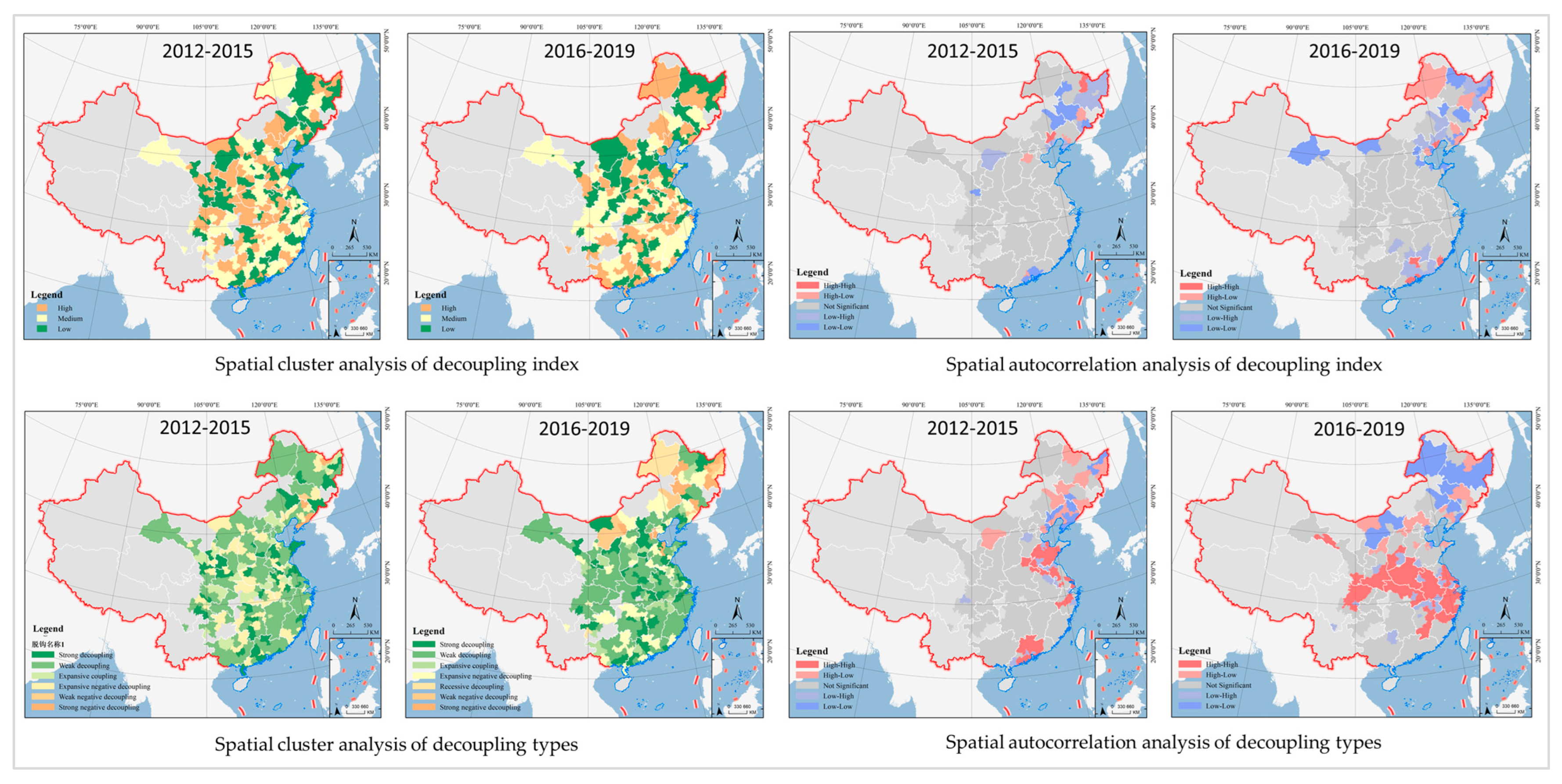
According to the analysis of the spatial clustering results, only the cities in strong and weak negative decoupling were clustered in the northeast region, while those in other types of decoupling were fragmented with no obvious spatial agglomerations. According to the spatial association analysis, from 2012 to 2015, HH cities were clustered in the eastern coastal regions such as Shandong, Jiangsu, Zhejiang and Guangdong, while LL and HL cities were concentrated in the northeast. HH cities expanded significantly from 2016 to 2019, and their spatial agglomeration level increased significantly. They were concentrated in a contiguous distribution in the Yangtze River Delta and its inland hinterland in the belt region, including Shanghai, Jiangsu, Zhejiang, Anhui, Henan, Hubei, Shaanxi and Sichuan. LL and HL cities were mainly concentrated in the north, including Heilongjiang, Jilin, Liaoning, Hebei and Inner Mongolia (Figure 8).

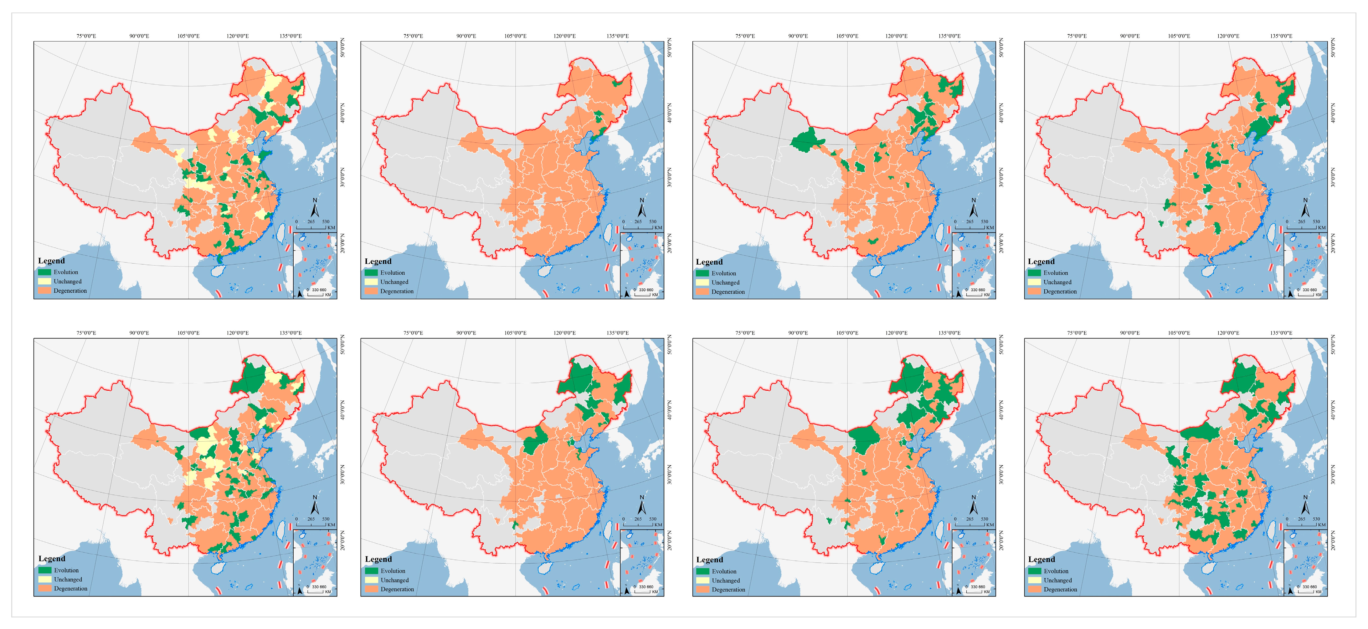
From the perspective of changes in decoupling type between 2012–2015 and 2016–2019, 91 cities achieved evolution, accounting for 33.33%, mostly located in central and north China. A total of 96 cities showed degeneration, accounting for 35.16%, and they were concentrated in the northeast region, but very scattered in other regions. There were 86 cities unchanged, accounting for 31.51%, mostly located in the eastern Yangtze River Delta and the west coast of the Strait region (Figure 9 and

Table 3. Statistical analysis of average annual growth rate.

		Service Industry Added Value		Gross Domestic Product		Service Industry Added Value
		2012–2015	2016–2019	2012–2015	2016–2019	2012–2015	2016–2019
Decoupling	Strong	51	54	44	51	42	43
	Weak	138	129	109	109	128	77
	Recessive	25	21	23	23	16	15
Coupling	Expansive	54	47	67	54	47	70
	Recessive	0	3	6	4	5	8
Negative Decoupling	Strong	0	0	1	1	1	2
	Weak	1	6	3	4	9	9
	Expansive	4	13	20	27	25	49

).

3.2.2. Urban Economy

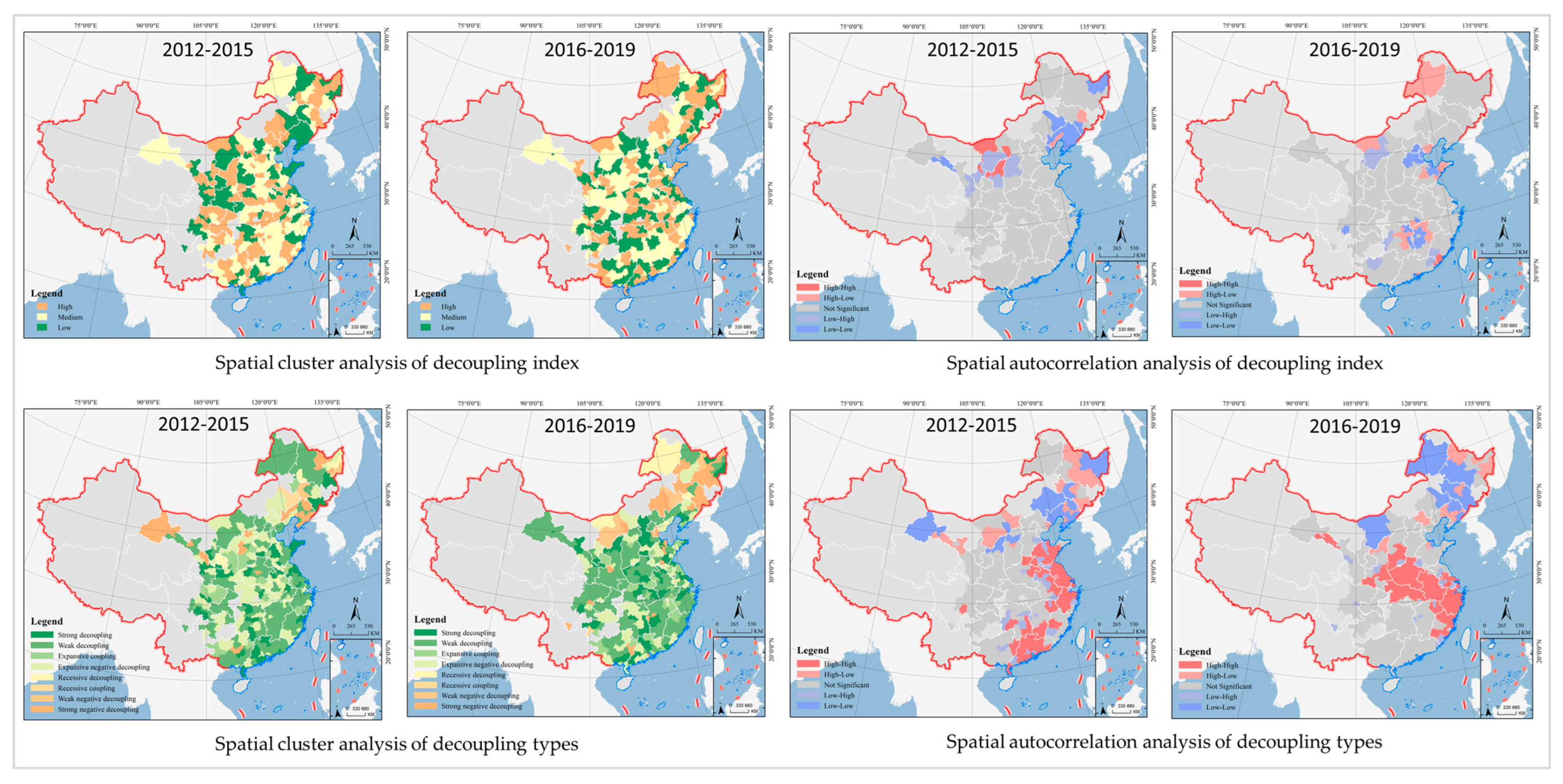
From the spatial clustering analysis of the decoupling indicator, cities of the high, medium and low levels were also fragmented in geographical distribution, with no obvious agglomerations. From the decoupling indicator correlation analysis, the global autocorrelation coefficient was 0.17 from 2012 to 2015 at 0.1 or a more stringent level of significance, and increased to 0.15 for 2016–2019, indicating that the spatial association was positive, but the spatial similarity and agglomeration level decreased slightly. From 2012 to 2015, HH cities were distributed in Inner Mongolia and Shaanxi Province, LL cities were distributed in Liaoning and Heilongjiang and LH cities were distributed in the fringe areas of HH cities. From 2016 to 2019, HH cities were distributed at the junction of Guangdong and Fujian, LL cities were clustered in Hebei and Jiangxi and HL cities were close to them.

In terms of decoupling types, all eight decoupling types emerged, with 40% in weak decoupling, about 20% in strong decoupling and expansive decoupling and nearly 10% in recessive decoupling and expansive negative decoupling. Strong and weak negative decoupling cities were concentrated in northeast China, which is becoming a problem area of concern and importance as the number of such cities continues to grow. Other types of cities were fragmented in distribution and there were no obvious spatial agglomerations. From the spatial association analysis, HH cities were concentrated and contiguous in zonal distribution in the eastern coastal region from 2012 to 2015, with the highest concentration in the Pearl River Delta and Yangtze River Delta. From 2016 to 2019, HH cities were highly clustered in the Yangtze River Delta and its inland hinterland region, covering Zhejiang, Jiangsu, Fujian, Anhui, Henan, Hubei and Shaanxi. LL and HL regions were mainly found in the north and highly concentrated in the northeast (Figure 10).

3.2.3. Government Revenue

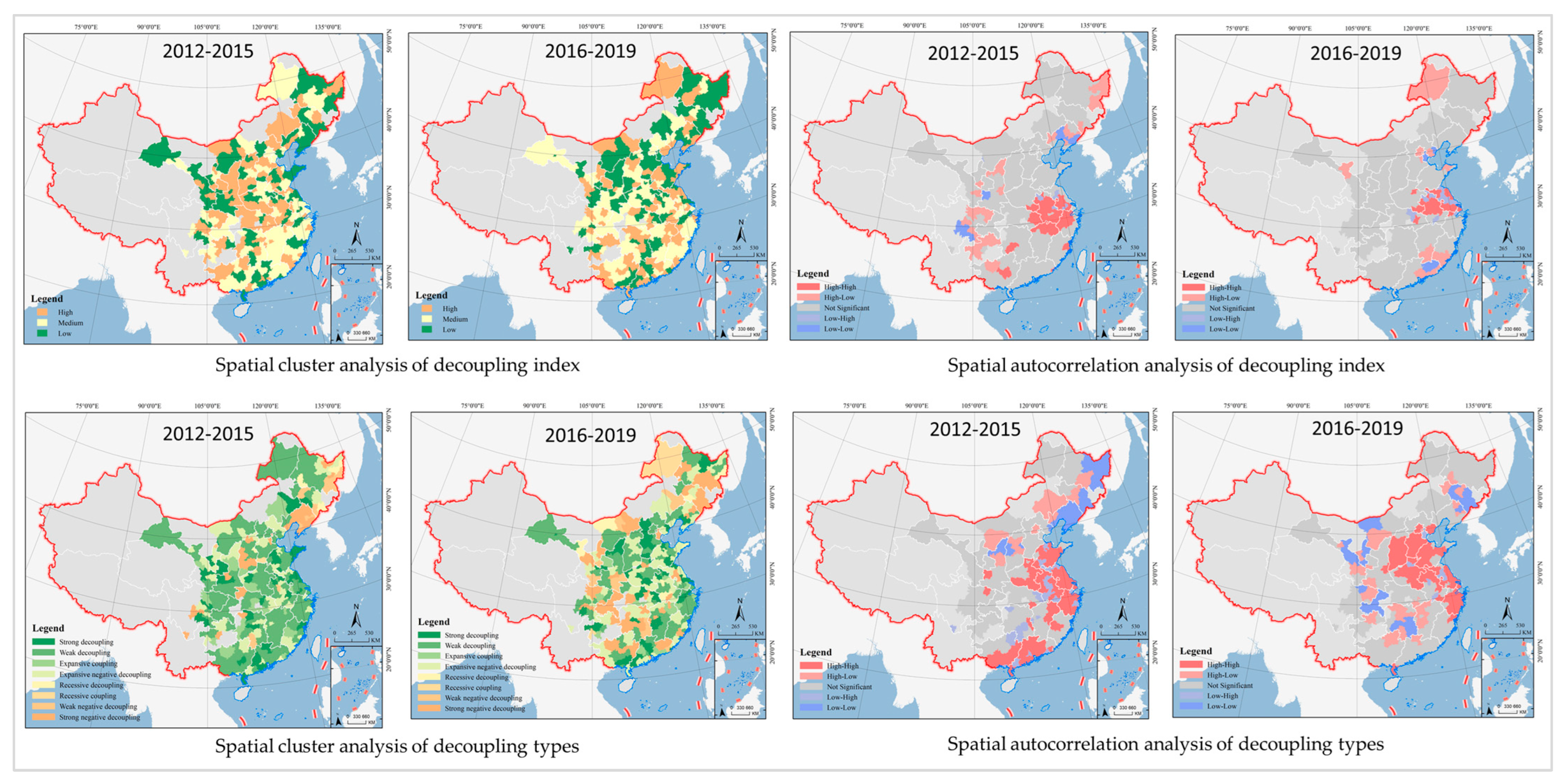
From the spatial clustering analysis of the decoupling indicator, from 2012 to 2015, the cities of high and medium levels were concentrated, with the former clustered in Hubei, Anhui and Shaanxi, while the latter clustered in Fujian, Jiangxi and Zhejiang. In the same period, the cities of a low level were scattered and there was no obvious agglomeration formed. From 2016 to 2019, the cities of high and low levels were fragmented in spatial distribution, while the cities of a medium level still maintained the trend of agglomeration. The coastal agglomeration of medium-level cities shrank moderately and new agglomerations were formed in the junctions of Chongqing, Hubei, Sichuan and Gansu in the west.

From the correlation analysis of the decoupling indicator, the global autocorrelation coefficient was 0.23 from 2012 to 2015 and increased to 0.10 from 2016 to 2019 at 0.1 or a more stringent level of significance, indicating a positive spatial association but gradually decreasing spatial similarity and agglomeration. From 2012 to 2015, HH cities were clustered in the Yangtze River Delta, while LL and HL cities formed two small agglomerations in the west and northeast, the former at the junctions of Sichuan, Shaanxi and Gansu, while the latter was in the coastal area of Liaoning and the border area of Heilongjiang. HH cities were concentrated in Jiangsu and Anhui from 2016 to 2019, but their spatial scope shrank. In the same period, there were a small number of HL and LL cities, mainly concentrated at the junction of Guangdong and Fujian and in the core area of Beijing–Tianjin–Hebei regions.

In terms of decoupling types, all eight types were present, with more cities in weak decoupling, strong decoupling and expansive coupling. The percentage of cities in weak decoupling decreased from 46.89% to 28.21%, those in expansive coupling increased from 17.22% to 25.64% and those in expansive negative decoupling increased from 9.16% to 17.95%, with the number of cities in unfavorable conditions continuing to grow.

Cities in states other than strong and weak negative decoupling were becoming increasingly fragmented in spatial distribution. Cities in strong and weak negative decoupling were mostly concentrated in the border region between China and North Korea from 2012 to 2015 and expanded to most of the northeast, northwest, central and western regions from 2016 to 2019. From the perspective of spatial association analysis, HH cities were concentrated and contiguous in the eastern coastal areas such as the Pearl River Delta, Yangtze River Delta and Shandong Peninsula from 2012 to 2015, forming two clusters, one large and one small, in south China and east China. From 2016 to 2019, the small cluster in south China disappeared while the large cluster in east China further expanded. LL and HL cities formed two clusters from 2012 to 2015 and expanded to four from 2016 to 2019. The former was located in the border region between China and North Korea, at the junction of Shaanxi, Shanxi and Inner Mongolia in the northeast; the latter covered the junctions of Gansu and Inner Mongolia, Chongqing and Sichuan, Hunan and its neighbors and Jilin and Liaoning. Specifically, the clusters in the northeast region shrank significantly (Figure 11).

In terms of decoupling type changes from 2012–2015 to 2016–2019, 81 cities experienced evolution, accounting for 29.67%. They were concentrated in Shaanxi, Hebei, Jilin and Shanxi but scattered in other regions. A total of 135 cities showed degeneration, accounting for 49.45%, widely distributed throughout the country, and therefore reasonable measures must be taken. There were 57 cities remaining unchanged, representing 20.88%, and they were also quite scattered across the country (Table 2 and Figure 9).

3.3. Influence Factors

3.3.1. Direct Driving Force

Decoupling is a key indicator in determining whether service economic development is independent of land resources. The previous analysis shows that for different cities the decoupling status varies greatly and there is a large spatial correlation effect. What are the driving mechanisms behind the formation and evolution of this phenomenon? To answer this question, we quantitatively measure the direct impact of each factor on decoupling and the interaction effects between different factors based on GeoDetector in this section to provide a basis for government policy design to promote more cities to move from a negative decoupling state to a decoupling state. In terms of the dependent variable, the previous analysis shows that the decoupling relationship between urban service land change and economic growth measured from different dimensions is somewhat different, and this paper works out the final decoupling effect by overlay analysis in accordance with the most unfavorable principle (

Table 4. Superposition analysis results of dependent variables.

Indicator	Code	Cities
Strong decoupling	4	Shijiazhuang, Handan, Baoding, Zhangjiakou, Hengshui, Anshan, Yingkou, Panjin, Hegang, Nantong, Lianyungang, Taizhou-jiangsu, Hangzhou, Jiaxing, Suzhou-anhui, Bozhou, Ji’an, Linyi, Binzhou, Pingdingshan, Jiaozuo, Puyang, Sanmenxia, Zhumadian, Ezhou, Jingmen, Huanggang, Suizhou, Loudi, Guangzhou, Shantou, Maoming, Qingyuan, Yunfu, Qinzhou, Yulin-guangxi, Leshan, Bijie, Yulin-shaanxi, Jiayuguan, Pingliang.
Weak decoupling	3	Beijing, Chengde, Cangzhou, Datong, Yangquan, Shuozhou, Yuncheng, Linfen, Lvliang, Jinzhou, Fuxin, Chaoyang, Heihe, Shanghai, Wuxi, Changzhou, Wenzhou, Huzhou, Shaoxing, Jinhua, Taizhou-zhejiang, Lishui, Hefei, Huaibei, Lu’an, Xuancheng, Xiamen, Putian, Sanming, Longyan, Ningde, Ganzhou, Yichun-jiangxi, Fuzhou-jiangxi, Wei fang, Kaifeng, Anyang, Hebi, Xuchang, Luohe, Shangqiu, Zhoukou, Huangshi, Shiyan, Yongzhou, Foshan, Nanning, Liuzhou, Guigang, Chengdu, Suining, Yibin, Dazhou, Ya’an, Guiyang, Baoji, Weinan, Yan’an, Hanzhong, Jinchang, Tianshui, Zhangye, Jiuquan.
Expansive coupling	2	Changzhi, Ningbo, Quzhou, Bengbu, Yingtan, Shangrao, Jingzhou, Huizhou, Shanwei, Nanchong, Anshun, Qingyang.
Expansive negative decoupling	1	Tangshan, Xingtai, Taiyuan, Jincheng, Jinzhong, Xinzhou, Shenyang, Dalian, Dandong, Tieling, Huludao, Changchun, Daqing, Suihua, Nanjing, Xuzhou, Suzhou-jiangsu, Yancheng, Zhenjiang, Suqian, Zhoushan, Wuhu, Maanshan, Huangshan, Chuzhou, Fuyang, Fuzhou-fujian, Zhangzhou, Nanping, Jiujiang, Jinan, Qingdao, Yantai, Jining, Tai’an, Rizhao, Dezhou, Liaocheng, Heze, Zhengzhou, Luoyang, Nanyang, Xinyang, Wuhan, Xiangyang, Xianning, Changsha, Changde, Zhangjiajie, Yiyang, Shaoguan, Shenzhen, Zhuhai, Jiangmen, Zhanjiang, Zhaoqing, Yangjiang, Dongguan, Chaozhou, Guilin, Beihai, Fangchenggang, Baise, Chongzuo, Zigong, Luzhou, Deyang, Bazhong, Zunyi, Tongchuan, Dingxi, Zhongwei.
Recessive decoupling	−1	Qinhuangdao, Bayannur, Siping, Jixi, Huainan, Tongling, Anqing, Weihai, Wuwei.
Recessive coupling	−2	Hulunbuir, Liupanshui.
Weak negative decoupling	−3	Baotou, Tongliao, Erdos, Benxi, Shuangyashan, Yichun-heilongjiang, Qitaihe, Zhuzhou, Chenzhou, Jieyang, Ankang, Shangluo, Longnan, Guyuan.
Strong negative decoupling	−4	Tianjin, Langfang, Hohhot, Wuhai, Chifeng, Ulanqab, Fushun, Liaoyang, Jilin Liaoyuan, Tonghua, Baishan, Songyuan, Baicheng, Harbin, Qiqihar, Jiamusi, Mudanjiang, Huai’an, Yangzhou, Chizhou, Quanzhou, Nanchang, Jingdezhen, Pingxiang, Xinyu, Zibo, Zaozhuang, Dongying, Xinxiang, Yichang, Xiaogan, Xiangtan, Hengyang, Shaoyang, Yueyang, Huaihua, Meizhou, Heyuan, Zhongshan, Wuzhou, Hezhou, Hechi, Laibin, Chongqing, Panzhihua, Mianyang, Guangyuan, Neijiang, Meishan, Guang’an, Ziyang, Tongren, Xi’an, Xianyang, Lanzhou, Baiyin, Yinchuan, Shizuishan, Wuzhong.

). In other words, the final decoupling status is the worst result among the three dimensions of service industry, urban economy and government revenue. For example, if the three dimensions have the analysis results of strong decoupling, weak decoupling and expansive coupling, respectively, the final decoupling is determined as expansive coupling. This approach allows the most rigorous analysis to be concluded and offers a higher reference value for government management.

For the independent variables, the quantile method is adopted for data discretization, and the best classification results are found by trial calculations for categories 2–11. When the independent variable is outside the best classification result, the q index becomes smaller or cannot pass the significance level test. According to the direct driving force analysis of the factors, we find the following: First, in terms of the significance level of influence, Government Financial Expenditure and International Trade pass the significance test of 0.05, and all the remaining factors pass the significance test of 0.03, indicating that all independent variables have a significant influence on decoupling. Second, in terms of driving force strength, Value Added of the Secondary Industry has the largest direct impact, followed by Urban Permanent Population, Total Retail of Commodities and Foreign Direct Investment above the average, with the remaining at the bottom, especially International Trade having the smallest value (

Table 5. Analysis on direct driving forces of factors.

Indicator	Code	Best Discretization	q Index	p Value
Urban Permanent Population	$X_1$	10	0.09	0.00
Value Added of the Secondary Industry	$X_2$	8	0.13	0.00
Per capita GDP	$X_3$	7	0.06	0.02
Government Financial Expenditure	$X_4$	6	0.04	0.05
International Trade	$X_5$	4	0.03	0.04
Foreign Direct Investment	$X_6$	10	0.07	0.02
Total Retail of Commodities	$X_7$	9	0.09	0.00
Authorized Patents	$X_8$	10	0.07	0.03

).

3.3.2. Interactive Driving Force

First of all, all the interactions of all factor pairs are of nonlinear enhancement, indicating significant synergy between different influencing factors. Secondly, the interactive driving forces vary considerably across factor pairs. Urban Permanent Population ∩ Value Added of the Secondary Industry, Urban Permanent Population ∩ Per capita GDP, Urban Permanent Population ∩ Foreign Direct Investment, Urban Permanent Population ∩ Total Retail of Commodities, Urban Permanent Population ∩ Authorized Patents, Foreign Direct Investment ∩ Value Added of the Secondary Industry, Foreign Direct Investment ∩ Per capita GDP, Per capita GDP ∩ Authorized Patents and Foreign Direct Investment ∩ Total Retail of Commodities have an interactive driving force over 0.3 times the direct driving force, so they are super interaction factor pairs (

Table 6. Analysis on interactive driving forces of factors.

	${\mathit{X}}_{\mathbf{1}}$	${\mathit{X}}_{\mathbf{2}}$	${\mathit{X}}_{\mathbf{3}}$	${\mathit{X}}_{\mathbf{4}}$	${\mathit{X}}_{\mathbf{5}}$	${\mathit{X}}_{\mathbf{6}}$	${\mathit{X}}_{\mathbf{7}}$
$X_2$	0.36
$X_3$	0.33	0.29
$X_4$	0.23	0.20	0.24
$X_5$	0.21	0.18	0.21	0.15
$X_6$	0.37	0.31	0.31	0.21	0.17
$X_7$	0.32	0.27	0.24	0.21	0.16	0.37
$X_8$	0.35	0.30	0.31	0.21	0.12	0.30	0.29

). Thirdly, the net synergy of the factor pairs can be measured by subtracting the direct driving force from the interactive driving force. Urban Permanent Population and Foreign Direct Investment lead in net synergies, while Value Added of the Secondary Industry, Per capita GDP, Authorized Patents and Total Retail of Commodities are above average, with the smallest values found for Government Financial Expenditure and International Trade (Figure 12).

4. Discussion

4.1. Design and Implement Differentiated Management Zones in Response to Spatial Effects

This paper finds significant spatial heterogeneity, agglomeration and correlation between service industry land and its economic growth in China, and it further corroborates some findings of the existing studies [68]. Shen [69] and Wang [70] conducted studies with the clustering and regression analysis method using Thiel’s coefficient, finding that China’s service industry has significant spatial differences, with economic development level, urban development scale and market capacity being the most important influencing factors. Liao [71] proposed the Concept Lattice Method for analyzing the spatial association of the service industry based on an empirical study of Nanning, China. Seo [72] also confirmed the high heterogeneity of service development in OECD countries and the impact of economies of scale and R&D expenditures on it. De [73] conducted a case study of Italy based on the Exploratory Spatial Data Analysis method and pointed out the high spatial concentration and dependence of the Italian service industry. Cook [74] conducted an empirical study on the UK and pointed out that service industry clusters vary significantly and those national policies are more conducive to cluster development than local policies.

It is necessary to strengthen the control of service industry land supply and improve the effect of urban land planning, construction and management, as a “one-size-fits-all” method is adopted in the current planning and plan management, approval management, land inspection and other control means, resulting in unsatisfactory management and control. Because of the significant spatial heterogeneity and agglomeration of urban service industry land change and their economic growth, different cities should be managed by classification for future service industry land use planning; furthermore, due to the significant spatial autocorrelation and correlation, urban synergy and regional cooperation should be taken into account during the management process, to design and build differentiated management zones based on spatial effects in the end. On the one hand, measures should be taken to implement differentiated and classified management of land use in different cities and industries, implement both rigid and elastic land use policies, and give priority to ensuring land supply in key cities, key industries and major projects [75]; on the other hand, local governments should encourage the establishment of regional urban service land trading platforms in the central cities of city clusters, metropolitan areas and economic zones, accurately identify community boundaries based on spatial correlation effects and promote land resource transactions and cooperation among different cities within the communities according to the needs of service economic development. In addition, it is also important to highlight the key management of unhealthy cities and regions in the future management of urban service industry land and take advantage of the new round of policy dividends and development opportunities to promote their healthy and sustainable development.

We should note that northeast China and northwest China have become the problem areas, where there are an increasing number of low-speed or even negative-growth cities, and spatial agglomerations of LL and HL cities have emerged. With the policy support of the Opinions on Several Major Policy Initiatives to Support the Revitalization of Northeast China in the Near Future, the northeast has been promoting the urban service industry upgrades and raising the proportion of service industry since 2014 and has realized the transformation and upgrading of the service industry and the conversion of development momentum [76]. However, the long-term lag in the expansion of service land and economic growth and the increasing number of cities in strong and weak negative decoupling have made the northeast and western regions key areas limiting the implementation of China’s coordinated regional development strategy.

Therefore, in the future, the northeast and western regions must seize the opportunity of China’s implementation of a new round of northeast revitalization and western development policies in urban service industry development and make policies according to local conditions and classification for different types of cities. Cities in the northeast and western regions should further accelerate the development of modern service industries, especially professional services, by taking advantage of the new opportunities given by the Western Development in China. At the central government level, the catalog of industries with advantages for foreign investment in central and western regions should be revised and dynamically adjusted in due course, and an industrial policy combining the negative list and the catalog of encouraged industries should be introduced to improve the precision and refinement of the policy [77,78]. At the local government level, it is necessary to implement the differentiated land use policy. For cities in the western and northeastern regions that are in decoupling, it is necessary to increase the scale of land supply and give preferential policy on the incremental construction land quota; additionally, it is necessary to strictly control the land supply in cities that are still in coupling and negative decoupling and innovate land use methods to improve the efficiency of land use.

4.2. Design and Implement Intensive Development Policies in Response to Decoupling Effects

This paper finds that most of the cities in China are in decoupling in terms of service industry land and economic growth, but 20% of the cities are still in coupling, and the number of cities in negative decoupling is increasing. From the type of decoupling relationship (rather than index), there is significant spatial clustering and autocorrelation between urban service industry land change and service industry added value, GDP and fiscal revenue growth, with two clusters forming in the Yangtze River Delta and Pearl River Delta in the early stage and mainly clustering in the Yangtze River Delta and its hinterland area in the later stage. In addition, from the perspective of the evolution of the decoupling type, the cities with a decoupling type in evolution, degeneration and unchanged states from 2012–2015 to 2016–2019 accounted for about 30%. In the context of slowing economic growth, special attention should be paid to the recoupling cities, and measures should be taken to reduce the possibility of recoupling between land use and economic development.

Improving the intensification of urban service industry land use, giving full play to the role of the government and the agglomerations it develops in boosting decoupling and promoting the formation of decoupling between urban service industry land and economic growth are key elements and prerequisites for achieving sustainable urban development, but they are not easy tasks. Liu [79] and Wu [80] believe that the government and its establishment of professional service industry clusters is an important factor affecting the level of spatial agglomeration and the development efficiency of the service industry. Therefore, it is suggested that the government should take the initiative to formulate a scientific and reasonable development plan for service industry clusters and introduce a series of incentive policies such as rent, tax and finance to guide service industry clusters and their intensive land use.

Modern service industry agglomeration is a specific industrial function area based on local characteristic resources and advantageous industries of the city, subject to unified planning, design and management according to the concept of the industrial cluster, relying on transportation hubs, industrial parks, historical and cultural neighborhoods, colleges and universities, science and technology parks and other spatial growth poles to promote the clustering and linked development of service industry enterprises and other concerned organizations. It is necessary to make overall plans for the agglomeration, incorporate the agglomeration into the economic and social development planning, master urban planning, land use planning and other special planning and implement it in a planned and step-by-step manner with major projects and leading enterprises as the core [81]. The agglomeration should promote the concentration of service industry enterprises of the same type in space, strengthen the supporting collaboration and professional division of labor in the industrial chain, enhance the public service capacity and give full play to the scale and spillover effects of industrial agglomeration. The government should set up a number of national-, provincial- and city-level modern service industry agglomerations by transforming and upgrading; cultivating and guiding; and planning and building new ones, with focus placed on cultivating new areas, upgrading advantageous areas, making bigger and stronger brands and development by industrial convergence, to establish a modern service industry agglomeration system with a reasonable planning layout, prominent industrial focus, obvious agglomeration benefits and strong radiation drive [82,83].

For agglomerations with a strong industrial base, sound development trend, great industry influence and high concentration of enterprise spatial layout, but with no effective socialized management, less informatization and modernization and the need to improve their ability of scientific and technological research and development, it is necessary to carry out transformation depending on advanced management and information technology, to improve the output and product technology content and enhance competitiveness and the development level. The agglomerations that represent the future direction of industrial development, weak industrial foundation and insufficient industrial influence but with fast development speed, high potential and obvious spatial agglomeration trend should be further accelerated through rational guidance, management upgrades and information transformation, so as to significantly improve their output efficiency and product competitiveness. For agglomerations with a small industry scale or development gap, but falling in the scope of special support by national and provincial policies and having a great impact on economic development with huge market potential, high industrial correlation and strong technological linkage function, it is necessary to provide infrastructure support through rational planning, introduce leading enterprises, drive the development of related industries and continuously create new growth points to promote economic development.

5. Conclusions

With the widespread application and expansion of decoupling theory, “decoupling” has gradually become a principal tool for exploring sustainable development. In a new era where more and more countries and cities are looking at service industry development as a strategic move to change their development model and economic structure, decoupling service industry land from economic growth has become a key measure of healthy urban development. Asia, especially China, is currently undergoing the transition from a manufacturing-based economy to a service-based economy, and its service industry is developing rapidly and has become a new engine of economic growth [84], making it a typical representative in the world. We empirically investigate the relationship between service industry land use and the economic growth in Chinese cities from 2012 to 2019 with a decoupling model. Findings were as follows:

(1) The spatial evolution of service industry land in Chinese cities is characterized by a high degree of heterogeneity and correlation, and it is becoming more significant. High-growth cities are becoming more geographically dispersed, while low-growth cities are increasingly clustered in the northeast and northwest regions.

(2) The change in the urban service economy in China is characterized by obvious cluster-like agglomeration. The increasing concentration of high- and low-growth cities in service industry added value, gross domestic product and government revenue and the long-term lagging urban development have made the northeast and northwest regions key problem areas limiting the implementation performance of China’s coordinated regional development strategy. HH cities are mainly clustered in the Yangtze River Delta, Pearl River Delta, Beijing–Tianjin–Hebei regions and Chengdu–Chongqing urban clusters, while LL and HL cities are mainly clustered in the north, especially in the northeast region.

(3) From 2012 to 2015 and 2016 to 2019, decoupling between service industry land expansion and economic growth in Chinese cities further enriched its types, and most cities were in weak decoupling, with evolution, degeneration and unchanged cities each accounting for one-third; there were a growing number of cities in negative decoupling, and the evolution of urban decoupling was becoming more diversified and complex.

(4) There is no significant spatial agglomeration in the decoupling indicator between urban service industry land and economic growth in China, but the decoupling type shows prominent spatial agglomeration and correlation; the agglomeration of HH cities is shifted from the eastern coastal contiguous zone to the coastal-to-inland contiguous zone, while LL and HL cities are clustered in the northeast and northwest regions for a long time.

(5) The decoupling relationship between urban service land change and economic growth is affected by many factors, and significant synergistic effects are found between different factors, mainly characterized by nonlinear enhancement. Notably, Value Added of the Secondary Industry has the largest direct driving force; Urban Permanent Population ∩ Value Added of the Secondary Industry and Urban Permanent Population ∩ Per capita GDP are among the super interaction factor pairs; and Urban Permanent Population and Foreign Direct Investment have a good lead in the net synergy.

(6) It is recommended to implement classified and differentiated urban land supply and utilization policies, especially to strengthen the management and control of service industry land in northeastern and northwestern cities. The central and local governments should work together to plan and build a group of national-, provincial- and city-level modern service industry clusters and take them as pilot areas to drive the change of the supply and use mode of urban service industry land, reduce the dependence of the service economy on land resources and improve the intensification of land development and utilization.

In theory, the decoupling model can effectively portray the dynamic relationship between urban service industry land expansion and economic growth and timely determine whether the relationship between land consumption and its economic output is in a reasonable state, providing a new method for researchers, government policy makers and the public to study the change pattern of urban service industry land and its driving mechanism. In practice, the methods and conclusions of this paper also provide valuable references for policy making in service industry land use planning and policy design in countries such as India, Egypt, Turkey, Russia and other countries similar to China.

There is a complex and variable relationship between urban service industry land and its economic growth under the influence of many factors. The decoupling model can help determine the level of service industry land use intensively in a concise and intuitive way, but it cannot directly demonstrate its impact mechanism, which is a shortcoming. In addition, given that a city may not be in the same decoupling state in the same period under different decoupling thresholds, the determination of decoupling results is a relative and dynamic process. Accordingly, the thresholds of decoupling indicators should be reasonably defined in the practical application, taking into account the actual situation, in order to further determine the decoupling state and formulate policies to deal with it, otherwise it will restrict the intensive use of urban service land and high-quality development.

It should be noted that decoupling analysis is stage-specific and policy-oriented, and there is no point in blindly pursuing decoupling. In view of the increasing number of cities with changes in service industry land and negative economic growth, it is necessary to be especially vigilant and prevent those in decoupling from recoupling in the context of economic transformation. Therefore, it is necessary to build a scientific and efficient management system for optimal allocation of land resources by taking targeted and adaptive policy measures in accordance with the development stage and policy needs, to gradually reduce the intensity of dependence on land resource consumption for service economic development and effectively enhance the capacity for high-quality urban economic development.

References

1. Lee, J.-W.; McKibbin, W.J. Service sector productivity and economic growth in Asia. Econ. Model. 2018, 74, 247–263. [Google Scholar] [CrossRef]
2. David, A.H. A service sector classification scheme using economic data. Serv. Ind. J. 2014, 34, 335–353. [Google Scholar] [CrossRef]
3. Eichengreen, B.; Gupta, P. The two waves of service-sector growth. Oxf. Econ. Pap. 2013, 65, 96–123. [Google Scholar] [CrossRef]
4. Li, Y.; Yuan, F. Business-promoted city-regionalism? New Industrial City projects by China Fortune Land Development. Reg. Stud. 2021, 56, 355–370. [Google Scholar] [CrossRef]
5. Borel-Saladin, J.; Crankshaw, O. Social Polarisation or Professionalisation? Another Look at Theory and Evidence on Deindustrialisation and the Rise of the Service Sector. Urban Stud. 2009, 46, 645–664. [Google Scholar] [CrossRef]
6. Meyssonnier, F. Service industry management control: A reflexion about its essence and tools. Comptab. Controle Audit. 2012, 18, 73–97. [Google Scholar] [CrossRef]
7. González-Cruz, T.F.; Roig-Tierno, N.; Botella-Carrubí, D. Quality management as a driver of innovation in the service industry. Serv. Bus. 2018, 12, 505–524. [Google Scholar] [CrossRef]
8. Gupta, S. Decoupling: A step toward sustainable development with reference to OECD countries. Int. J. Sustain. Dev. World Ecol. 2015, 22, 510–519. [Google Scholar] [CrossRef]
9. Guo, S.; Liu, L.; Zhao, Y. The business cycle implications of land financing in China. Econ. Model. 2015, 46, 225–237. [Google Scholar] [CrossRef]
10. Liao, J. The rise of the service sector in China. China Econ. Rev. 2020, 59, 101385. [Google Scholar] [CrossRef]
11. Wang, L.; Yuan, F.; Duan, X. How high-speed rail service development influenced commercial land market dynamics: A case study of Jiangsu province, China. J. Transp. Geogr. 2018, 72, 248–257. [Google Scholar] [CrossRef]
12. Shao, S.; Tian, Z.; Yang, L. High speed rail and urban service industry agglomeration: Evidence from China’s Yangtze River Delta region. J. Transp. Geogr. 2017, 64, 174–183. [Google Scholar] [CrossRef]
13. Tian, M.; Li, T.; Yang, S.; Wang, Y.; Fu, S. The Impact of High-Speed Rail on the Service-Sector Agglomeration in China. Sustainability 2019, 11, 2128. [Google Scholar] [CrossRef]
14. Tian, M.; Li, T.; Ye, X.; Zhao, H.; Meng, X. The impact of high-speed rail on service industry agglomeration in peripheral cities. Transp. Res. Part D Transp. Environ. 2021, 93, 102745. [Google Scholar] [CrossRef]
15. Yang, L.Y.; Hu, L.Q.; Shang, P.; Ye, Y.M. Estimating the Impacts of High-speed Rail on Service Industry Agglomeration in China. J. Transp. Econ. Policy 2021, 55, 16–35. [Google Scholar]
16. Sheng, J.; Xu, H.; Zheng, J.; Luo, M.; Zhou, X. Commercial Value Assessment of “Grey Space” under Overpasses: Analytic Hierarchy Process. Adv. Civ. Eng. 2018, 2018, 4970697. [Google Scholar] [CrossRef]
17. Yang, H.J.; Song, J.; Choi, M.J. Measuring the Externality Effects of Commercial Land Use on Residential Land Value: A Case Study of Seoul. Sustainability 2016, 8, 432. [Google Scholar] [CrossRef]
18. Sohn, D.-W. Do all commercial land uses deteriorate neighborhood safety?: Examining the relationship between commercial land-use mix and residential burglary. Habitat Int. 2016, 55, 148–158. [Google Scholar] [CrossRef]
19. Browning, C.R.; Byron, R.A.; Calder, C.A.; Krivo, L.J.; Kwan, M.-P.; Lee, J.-Y.; Peterson, R.D. Commercial Density, Residential Concentration, and Crime: Land Use Patterns and Violence in Neighborhood Context. J. Res. Crime Delinq. 2010, 47, 329–357. [Google Scholar] [CrossRef]
20. Izanloo, A.; Rafsanjani, A.K.; Ebrahimi, S.P. Effect of Commercial Land Use and Accessibility Factor on Traffic Flow in Bojnourd. J. Urban Plan. Dev. 2017, 143, 05016016. [Google Scholar] [CrossRef]
21. Langer, S.; Korzhenevych, A. The effect of industrial and commercial land consumption on municipal tax revenue: Evidence from Bavaria. Land Use Policy 2018, 77, 279–287. [Google Scholar] [CrossRef]
22. Nichols, J.B.; Oliner, S.D.; Mulhall, M.R. Swings in commercial and residential land prices in the United States. J. Urban Econ. 2013, 73, 57–76. [Google Scholar] [CrossRef]
23. Garang, Z.; Wu, C.; Li, G.; Zhuo, Y.; Xu, Z. Spatio-Temporal Non-Stationarity and Its Influencing Factors of Commercial Land Price: A Case Study of Hangzhou, China. Land 2021, 10, 317. [Google Scholar] [CrossRef]
24. Ustaoglu, E.; Silva, F.B.E.; LaValle, C. Quantifying and modelling industrial and commercial land-use demand in France. Environ. Dev. Sustain. 2020, 22, 519–549. [Google Scholar] [CrossRef]
25. Silva, F.B.E.; Koomen, E.; Diogo, V.; Lavalle, C. Estimating Demand for Industrial and Commercial Land Use Given Economic Forecasts. PLoS ONE 2014, 9, e91991. [Google Scholar] [CrossRef]
26. Wiedenhofer, D.; Virág, D.; Kalt, G.; Plank, B.; Streeck, J.; Pichler, M.; Mayer, A.; Krausmann, F.P.; Brockway, P.; Schaffartzik, A.; et al. A systematic review of the evidence on decoupling of GDP, resource use and GHG emissions, part I: Bibliometric and conceptual mapping. Environ. Res. Lett. 2020, 15, 063002. [Google Scholar] [CrossRef]
27. Haberl, H.; Wiedenhofer, D.; Virág, D.; Kalt, G.; Plank, B.; Brockway, P.; Fishman, T.; Hausknost, D.; Krausmann, F.; Leon-Gruchalski, B.; et al. A systematic review of the evidence on decoupling of GDP, resource use and GHG emissions, part II: Synthesizing the insights. Environ. Res. Lett. 2020, 15, 065003. [Google Scholar] [CrossRef]
28. Wang, T.; Riti, J.S.; Shu, Y. Decoupling emissions of greenhouse gas, urbanization, energy and income: Analysis from the economy of China. Environ. Sci. Pollut. Res. 2018, 25, 19845–19858. [Google Scholar] [CrossRef]
29. Frodyma, K.; Papież, M.; Śmiech, S. Decoupling Economic Growth from Fossil Fuel Use—Evidence from 141 Countries in the 25-Year Perspective. Energies 2020, 13, 6671. [Google Scholar] [CrossRef]
30. Yasmeen, H.; Tan, Q. Assessing Pakistan’s energy use, environmental degradation, and economic progress based on Tapio decoupling model. Environ. Sci. Pollut. Res. 2021, 28, 68364–68378. [Google Scholar] [CrossRef]
31. Szigeti, C.; Toth, G.; Szabo, D.R. Decoupling—shifts in ecological footprint intensity of nations in the last decade. Ecol. Indic. 2017, 72, 111–117. [Google Scholar] [CrossRef]
32. Dong, F.; Li, J.; Zhang, X.; Zhu, J. Decoupling relationship between haze pollution and economic growth: A new decoupling index. Ecol. Indic. 2021, 129, 107859. [Google Scholar] [CrossRef]
33. Dong, F.; Li, J.; Li, K.; Sun, Z.; Yu, B.; Wang, Y.; Zhang, S. Causal chain of haze decoupling efforts and its action mechanism: Evidence from 30 provinces in China. J. Clean. Prod. 2020, 245, 118889. [Google Scholar] [CrossRef]
34. Qian, Y.; Cao, H.; Huang, S. Decoupling and decomposition analysis of industrial sulfur dioxide emissions from the industrial economy in 30 Chinese provinces. J. Environ. Manag. 2020, 260, 110142. [Google Scholar] [CrossRef]
35. Chen, J.; Wang, P.; Cui, L.; Huang, S.; Song, M. Decomposition and decoupling analysis of CO2 emissions in OECD. Appl. Energy 2018, 231, 937–950. [Google Scholar] [CrossRef]
36. Mikayilov, J.I.; Hasanov, F.J.; Galeotti, M. Decoupling of CO2 emissions and GDP: A time-varying cointegration approach. Ecol. Indic. 2018, 95, 615–628. [Google Scholar] [CrossRef]
37. Adalibieke, W.; Zhan, X.; Cui, X.; Reis, S.; Winiwarter, W.; Zhou, F. Decoupling between ammonia emission and crop production in China due to policy interventions. Glob. Chang. Biol. 2021, 27, 5877–5888. [Google Scholar] [CrossRef]
38. Lundquist, S. Explaining events of strong decoupling from CO2 and NOx emissions in the OECD 1994–2016. Sci. Total. Environ. 2021, 793, 148390. [Google Scholar] [CrossRef]
39. Shi, Y.B.; Zhao, X.X.; Jang, C.-L.; Chang, C.-P. Decoupling effect between economic development and environmental pollution: A spatial-temporal investigation using 31 provinces in China. Energy Environ. 2019, 30, 755–775. [Google Scholar] [CrossRef]
40. Chen, X.; Pang, J.; Zhang, Z.; Li, H. Sustainability Assessment of Solid Waste Management in China: A Decoupling and Decomposition Analysis. Sustainability 2014, 6, 9268–9281. [Google Scholar] [CrossRef]
41. Wang, L.; Cutforth, H.; Lal, R.; Chai, Q.; Zhao, C.; Gan, Y.; Siddique, K.H. ‘Decoupling’ land productivity and greenhouse gas footprints: A review. Land Degrad. Dev. 2018, 29, 4348–4361. [Google Scholar] [CrossRef]
42. Zhang, Z.; Hu, B.; Shi, K.; Su, K.; Yang, Q. Exploring the dynamic, forecast and decoupling effect of land natural capital utilization in the hinterland of the Three Gorges Reservoir area, China. Sci. Total. Environ. 2020, 718, 134832. [Google Scholar] [CrossRef] [PubMed]
43. Shao, J.; Ge, J. Investigation into Relationship between Intensive Land Use and Urban Heat Island Effect in Shijiazhuang City Based on the Tapio Decoupling Theory. J. Urban Plan. Dev. 2020, 146, 04020043. [Google Scholar] [CrossRef]
44. Li, Y.-N.; Cai, M.; Wu, K.; Wei, J. Decoupling analysis of carbon emission from construction land in Shanghai. J. Clean. Prod. 2019, 210, 25–34. [Google Scholar] [CrossRef]
45. Li, M.; Shi, Y.; Duan, W.; Chen, A.; Wang, N.; Hao, J. Spatiotemporal Decoupling of Population, Economy and Construction Land Changes in Hebei Province. Sustainability 2019, 11, 6794. [Google Scholar] [CrossRef]
46. Wang, C.; Liu, Y.; Kong, X.; Li, J. Spatiotemporal Decoupling between Population and Construction Land in Urban and Rural Hubei Province. Sustainability 2017, 9, 1258. [Google Scholar] [CrossRef]
47. Liu, Y.; Cai, E.; Jing, Y.; Gong, J.; Wang, Z. Analyzing the Decoupling between Rural-to-Urban Migrants and Urban Land Expansion in Hubei Province, China. Sustainability 2018, 10, 345. [Google Scholar] [CrossRef]
48. Guo, S.; Wang, Y.; Huang, J.; Dong, J.; Zhang, J. Decoupling and Decomposition Analysis of Land Natural Capital Utilization and Economic Growth: A Case Study in Ningxia Hui Autonomous Region, China. Int. J. Environ. Res. Public Health 2021, 18, 646. [Google Scholar] [CrossRef]
49. Imbrogiano, J.-P. Contingency in Business Sustainability Research and in the Sustainability Service Industry: A Problematization and Research Agenda. Organ. Environ. 2020, 34, 298–322. [Google Scholar] [CrossRef]
50. Zhang, P.; Li, W.; Zhao, K.; Zhao, S. Spatial Pattern and Driving Mechanism of Urban–Rural Income Gap in Gansu Province of China. Land 2021, 10, 1002. [Google Scholar] [CrossRef]
51. Li, W.; Zhang, P.; Zhao, K.; Chen, H.; Zhao, S. The Evolution Model of and Factors Influencing Digital Villages: Evidence from Guangxi, China. Agriculture 2023, 13, 659. [Google Scholar] [CrossRef]
52. Organization for Economic Cooperation and Development. Indicators to Measure Decoupling of Environmental Pressure and Economic Growth; OECD: Paris, France, 2000.
53. Casadio Tarabusi, E.C.; Guarini, G. An axiomatic approach to decoupling indicators for green growth. Ecol. Indic. 2018, 84, 515–524. [Google Scholar] [CrossRef]
54. Pesce, A. THE DECOUPLING OF EMERGING ECONOMIES: THEORETICAL AND EMPIRICAL PUZZLE. J. Econ. Surv. 2017, 31, 602–631. [Google Scholar] [CrossRef]
55. Tapio, P. Towards a theory of decoupling: Degrees of decoupling in the EU and the case of road traffic in Finland between 1970 and 2001. Transp. Policy 2005, 12, 137–151. [Google Scholar] [CrossRef]
56. Huang, Y.; Zhang, J.; Wu, J. Integrating Sustainability Assessment into Decoupling Analysis: A Focus on the Yangtze River Delta Urban Agglomerations. Sustainability 2020, 12, 7872. [Google Scholar] [CrossRef]
57. Longhofer, W.; Jorgenson, A. Decoupling reconsidered: Does world society integration influence the relationship between the environment and economic development? Soc. Sci. Res. 2017, 65, 17–29. [Google Scholar] [CrossRef]
58. Eswaran, M.; Kotwal, A. The role of the service sector in the process of industrialization. J. Dev. Econ. 2002, 68, 401–420. [Google Scholar] [CrossRef]
59. Rahman, M.; Kamal, M.M.; Aydin, E.; Haque, A.U. Impact of Industry 4.0 drivers on the performance of the service sector: Comparative study of cargo logistic firms in developed and developing regions. Prod. Plan. Control. 2020, 33, 228–243. [Google Scholar] [CrossRef]
60. Song, Y.; Sun, J.; Zhang, M.; Su, B. Using the Tapio-Z decoupling model to evaluate the decoupling status of China’s CO2 emissions at provincial level and its dynamic trend. Struct. Chang. Econ. Dyn. 2020, 52, 120–129. [Google Scholar] [CrossRef]
61. Lu, Z.; Wang, H.; Yue, Q. Decoupling Analysis of the Environmental Mountain-with Case Studies from China. J. Ind. Ecol. 2015, 19, 1082–1090. [Google Scholar] [CrossRef]
62. Zhao, S.; Li, W.; Zhao, K.; Zhang, P. Change Characteristics and Multilevel Influencing Factors of Real Estate Inventory—Case Studies from 35 Key Cities in China. Land 2021, 10, 928. [Google Scholar] [CrossRef]
63. Wang, J.-F.; Li, X.-H.; Christakos, G.; Liao, Y.-L.; Zhang, T.; Gu, X.; Zheng, X.-Y. Geographical detectors-based health risk assessment and its application in the neural tube defects study of the Heshun region, China. Int. J. Geogr. Inf. Sci. 2010, 24, 107–127. [Google Scholar] [CrossRef]
64. Guan, X.Y.; Wang, S.L.; Gao, Z.Y.; Lv, Y.; Fu, X.J. Spatio-temporal variability of soil salinity and its relationship with the depth to groundwater in salinization irrigation district. Acta Ecol. Sin. 2012, 32, 198–206. [Google Scholar]
65. Liu, X.N.; Huang, F.; Wang, P. Spatial Analysis Principle and Method of GIS; Science Press: Beijing, China, 2008; pp. 199–206. [Google Scholar]
66. Miyamoto, S.; Chacon, A.; Hossain, M.; Martinez, L. Soil salinity of urban turf areas irrigated with saline water I. Spatial variability. Landsc. Urban Plan. 2005, 71, 233–241. [Google Scholar]
67. She, D.L.; Shao, M.A.; Yu, S.G. Spatial Variability of Soil Water Content on a Cropland-grassland Mixed Slope Land in the Loess Plateau, China. Trans. Chin. Soc. Agric. Mach. 2010, 41, 57–63. [Google Scholar]
68. Na, J.; Lee, J.-D.; Baek, C. Is the service sector different in size heterogeneity? J. Econ. Interact. Co-Ord. 2017, 12, 95–120. [Google Scholar] [CrossRef]
69. Shen, Y.; Qiu, L.; Ren, W.; Cao, Y.; Hu, D.; Song, Y. Basic characteristics, spatial disparity and its major influencing factors of service industry in China. Chin. Geogr. Sci. 2009, 19, 314–324. [Google Scholar] [CrossRef]
70. Wang, E. The Service Sector in the Chinese Economy: A Geographic Appraisal. Eurasian Geogr. Econ. 2009, 50, 275–300. [Google Scholar] [CrossRef]
71. Liao, W.; Zhang, Z.; Jiang, W. Concept Lattice Method for Spatial Association Discovery in the Urban Service Industry. ISPRS Int. J. Geo-Inf. 2020, 9, 155. [Google Scholar] [CrossRef]
72. Seo, H.J.; Lee, Y.S.; Kim, H.S. Technological Change and Service Industry Market Share. J. Korea Trade 2013, 17, 1–28. [Google Scholar]
73. De Dominicis, L.; Arbia, G.; De Groot, H.L. Concentration of Manufacturing and Service Sector Activities in Italy: Accounting for Spatial Dependence and Firm Size Distribution. Reg. Stud. 2013, 47, 405–418. [Google Scholar] [CrossRef]
74. Cook, G.A.; Pandit, N.R. Service Industry Clustering: A Comparison of Broadcasting in Three City-Regions. Serv. Ind. J. 2007, 27, 453–469. [Google Scholar] [CrossRef]
75. Hu, Y.; Wang, M. Impact of resource reconfiguration on total factor productivity of service industry. Int. J. Electr. Eng. Educ. 2020, 0020720920940579. [Google Scholar] [CrossRef]
76. Guan, W.; Cao, J.B.; Xu, S.T. The Evolution of the Development Space Polarization and Driving Factors in the Service Industry in Northeast China. Sci. Geogr. Sin. 2015, 35, 733–741. [Google Scholar] [CrossRef]
77. Jia, J.; Ma, G.; Qin, C.; Wang, L. Place-based policies, state-led industrialisation, and regional development: Evidence from China’s Great Western Development Programme. Eur. Econ. Rev. 2020, 123, 103398. [Google Scholar] [CrossRef]
78. Li, P.; Tian, Y.; Wu, J.; Xu, W. The Great Western Development policy: How it affected grain crop production, land use and rural poverty in western China. China Agric. Econ. Rev. 2021, 13, 319–348. [Google Scholar] [CrossRef]
79. Liu, J.; Zhao, M. Study on Evolution and Interaction of Service Industry Agglomeration and Efficiency of Hebei Province China. Complexity 2020, 2020, 1750430. [Google Scholar] [CrossRef]
80. Wu, Y.; Fan, P.; You, H. Spatial Evolution of Producer Service Sectors and Its Influencing Factors in Cities: A Case Study of Hangzhou, China. Sustainability 2018, 10, 975. [Google Scholar] [CrossRef]
81. Chiming, G.; Qian, W. Planning of Service Industry Agglomeration Area from the Perspectives of Geographical Space and Industrial Organization: A Case Study on Changzhou, Jiangsu Province. City Plan. Rev. 2016, 40, 33–42. [Google Scholar] [CrossRef]
82. Dong, O.; Sidong, Z.; Yaoping, X.; Lin, L.; Cunbin, Z. Theory and Practice of Modern Productive Service Concentration Development Planning, Guangxi. Planners 2015, 31, 30–36. [Google Scholar]
83. Xi, C.; Bin, L. The Development Patterns of Service Cluster in Small and Medium-Sized Cities. Econ. Geogr. 2014, 34, 105–111. [Google Scholar] [CrossRef]
84. Kim, J.; Wood, J. Service sector development in Asia: An important instrument of growth. Asian-Pac. Econ. Lit. 2020, 34, 12–25. [Google Scholar] [CrossRef]
Figure 1. Study Area.
Land 12 01139 g001
Figure 2. Research steps.
Land 12 01139 g002
Figure 3. Decoupling type and decoupling indicator range.
Land 12 01139 g003
Figure 4. Factor and interaction detector of GeoDetector.
Land 12 01139 g004
Figure 5. Spatial cluster analysis.
Land 12 01139 g005
Figure 6. Analysis on the change trend of service industry land use and output.
Land 12 01139 g006
Figure 7. Spatial autocorrelation analysis.
Land 12 01139 g007
Figure 8. Analysis on decoupling of service economy.
Land 12 01139 g008
Figure 9. Analysis on change of decoupling types.
Land 12 01139 g009
Figure 10. Analysis on decoupling of urban economy.
Land 12 01139 g010
Figure 11. Analysis on decoupling of government revenue.
Land 12 01139 g011
Figure 12. Analysis on net synergistic effect of factors.
Land 12 01139 g012