Testing the Effect of Relative Pollen Productivity on the REVEALS Model: A Validated Reconstruction of Europe-Wide Holocene Vegetation

Abstract

Reliable quantitative vegetation reconstructions for Europe during the Holocene are crucial to improving our understanding of landscape dynamics, making it possible to assess the past effects of environmental variables and land-use change on ecosystems and biodiversity, and mitigating their effects in the future. We present here the most spatially extensive and temporally continuous pollen-based reconstructions of plant cover in Europe (at a spatial resolution of 1° × 1°) over the Holocene (last 11.7 ka BP) using the ‘Regional Estimates of VEgetation Abundance from Large Sites’ (REVEALS) model. This study has three main aims. First, to present the most accurate and reliable generation of REVEALS reconstructions across Europe so far. This has been achieved by including a larger number of pollen records compared to former analyses, in particular from the Mediterranean area. Second, to discuss methodological issues in the quantification of past land cover by using alternative datasets of relative pollen productivities (RPPs), one of the key input parameters of REVEALS, to test model sensitivity. Finally, to validate our reconstructions with the global forest change dataset. The results suggest that the RPPs.st1 (31 taxa) dataset is best suited to producing regional vegetation cover estimates for Europe. These reconstructions offer a long-term perspective providing unique possibilities to explore spatial-temporal changes in past land cover and biodiversity.

1. Introduction

The IPBES 2019 global report ranked changes in land use and land cover as the greatest drivers of declines in nature and biodiversity [1]. Anthropogenic biodiversity decline and anthropogenic climate change have largely been driven by the direct exploitation of nature through deforestation and conversion for agriculture and livestock production (IPBES, [1,2]). Loss of biodiversity and the transformation of nature by humans are often considered to be recent impacts on the environment, stretching over recent decades and centuries, and reflected in instrumental records and detailed ecological surveys. However, the reshaping of terrestrial nature began in the Paleolithic and Mesolithic ages, with practices including hunting, fishing, and gathering having the potential to modify existing ecosystem systems at localized scales through, for example, selective gathering or depleting of local resources [3,4,5,6]. Forest clearance for agriculture started at least 6000 years ago in western Europe and probably earlier in the regions in which agriculture developed [7]. Sustainable practices over time took the form of appropriation, colonization, and land-use intensification, which led to ecosystem transformations [8]. The intensification of human activities and the loss of sustainable practices make Europe one of the regions of the world where human-induced effects on vegetation are most notable [7]. The increments of species extinction, soil erosion, altered biogeochemical processes, fire frequency, and hydrology left long-term legacies across the biosphere and shaped most of terrestrial nature for at least 12,000 years [8]. A worldwide acceleration in the rates of vegetation compositional change starting between 4600 and 2900 years ago was demonstrated using a global set of over 1000 fossil pollen records and a new method to estimate the “rate of change” [9]. This human-induced acceleration was shown to exceed the climate-driven transformations of the last deglaciation. This study highlights past land use and environmental forcings legacies in relation to the strong anthropogenic imprint of the past decades on contemporary communities and biodiversity trends. Times of technological development (e.g., the introduction of metals, innovations in plough shape, new cropping systems) transformed ecological structures and dynamics, including vegetation (impacting species richness, evenness, and biomass), which led to progressive replacement of semi-natural or natural ecosystems by human-modified ones [3,9,10,11]. In order to fully understand past and contemporary ecological processes, rates of biodiversity changes, and ecological thresholds at continental scales and globally, it is essential to have an overview of long-term land-cover dynamics [12,13,14,15,16,17,18].

Attempts to reconstruct past land cover have been made to model land-use and land-cover change (LULCC) over Holocene time scales (e.g., HYDE 3.2 [19] and KK10 [20]). Such LULCC scenarios have been used in combination with dynamic vegetation models to understand interactions between different components of the Earth system in the past (Earth system modeling (ESM), [21]). However, there can be considerable disagreement between different LULCC scenarios, and this highlights the need to use independent and empirical datasets of land use and land cover [22]. Pollen archives remain the best empirical data to address differences between LULCC scenarios, as they provide a direct proxy for vegetation cover [22,23,24,25].

Efforts to improve our understanding of past vegetation using pollen have led to the development of models that correct the non-linear pollen–vegetation relationship and can compensate for plant taxon-specific differences in pollen production, dispersal, and deposition [26,27]. Currently, the ‘Regional Estimates of VEgetation Abundance from Large Sites’ (REVEALS) model is the most appropriate method to reconstruct plant cover at a regional spatial scale of ca. 100 km × 100 km [27]. The REVEALS model was developed to transform pollen data from large lakes but can also produce regional vegetation cover estimates from multiple small-sized sites [27,28,29,30].

The REVEALS model has previously been applied at regional to continental scale. Githumbi et al. (2022) published the most detailed estimates of past plant cover across Europe and part of the eastern Mediterranean–Black Sea–Caspian corridor [31]. REVEALS reconstructions were performed at a spatial scale of 1° × 1° (grid cell of ca. 100 km × 100 km) and a temporal resolution of 500 years between 11.7 and 0.7 ka BP, and three shorter time windows (0.7−0.35 ka BP, 0.35−0.1 ka BP, and 0.1 ka BP−present) for use in climate modeling studies (e.g., [32]). The accuracy and reliability of gridded REVEALS estimates have been discussed in several studies [28,31,33,34]. Gridded REVEALS estimates are influenced by the quality of individual records used (pollen count size, taxonomic resolution, and chronological uncertainty), basin size, and type of sites (lakes or bogs), the number of pollen records used in each grid cell, and the reliability of the relative pollen productivities (RPPs) used. Where gridded REVEALS estimates are based on low numbers of small sites, there is greater uncertainty in the reliability of the REVEALS estimates; if the RPPs for taxa that are considered important components of the regional vegetation are based on limited empirical studies, this can further impact the quality of the estimates. For instance, more work has been undertaken on RPPs of temperate and boreal taxa than those that characterize the Mediterranean region.

RPPs and their standard deviations exist for more than 131 Northern Hemisphere taxa, with the longest research effort in Europe, and several syntheses of RPPs have been published [28,31,34,35,36]. As the REVEALS model assumes that RPP values are constant within the region of interest and through time [27], studies working at the sub-continental scale have calculated mean RPPs considering all available RPP values. This can overcome the variability of RPP estimates within one taxon. Mazier et al. (2012) produced the first RPP-means dataset for Europe [28], comprising 25 pollen taxa that were used in the “first generation” of REVEALS reconstruction for Europe [33]. Githumbi et al. (2022) published an updated RPP-mean dataset for 50 taxa from Europe [31]. Thirty-nine of the taxa were from boreal and temperate Europe, and for the first time, 11 taxa characteristic of Mediterranean Europe were included.

The first RPP-mean dataset for Europe was used to evaluate the effect of entomophilous taxa on gridded REVEALS estimates for the Czech Republic [28]. The authors showed that entomophilous taxa tend to affect the REVEALS estimates because the REVEALS model assumes that all pollen is airborne [27] and justified excluding as many entomophilous taxa as possible from REVEALS reconstructions. Githumbi et al. (2022) included taxa with mixed wind and insect pollen transport such as Artemisia, Amaranthaceae/Chenopodiaceae, Ericaceae (Calluna excluded), Rubiaceae, and Plantago lanceolata [31]. The application of multiple sets of RPP values for different climatic regions in a single REVEALS reconstruction cannot be achieved without independent data on past climatic changes, which can shift the boundaries between climate regimes over the Holocene [31]. Some taxa are more difficult to handle, such as the family Ericaceae, which contains a morphologically diverse range of taxa, including herbs, dwarf shrubs, shrubs, and trees [37]. Only two RPP values across Europe are available for Ericaceae [31]. The first is from the Mediterranean area, where Ericaceae species are mainly tree forms, produce abundant pollen, and therefore have a high RPP. The second is based on low-growth shrubs in northern Europe and has a lower RPP value than that from the Mediterranean.

In this paper, we use an updated version of the REVEALS reconstruction from [31]. This third generation produces grid-based estimates at 1° × 1° (ca. 100 km × 100 km) across 30°–71° N, 20° W–47° E (northwestern, central Europe, Mediterranean area, and part of the East until 47° E, Figure 1 and Figure A1) for 25 contiguous time windows across the Holocene. The number of pollen records used (1607) and the area covered (most of Europe) of 539 grid cells represent a significant advance on the results presented by [31], which was based on 1128 pollen records for Europe and part of the Eastern Mediterranean–Black Sea–Caspian-Corridor. We used three RPP-means datasets and evaluated the extent to which the selection of a set of RPP-means influences the REVEALS estimates. The three datasets are (i) the RPP-means dataset from [31] (RPPs.st1: 31 taxa); (ii) a new synthesis proposed in this study inclusive of a larger number of entomophilous taxa (RPPs.st2: 46 taxa); and (iii) a composite dataset, derived from [28,31] (RPPs.st3: 31 taxa).

The specific aims of this paper are: (1) to improve the accuracy and reliability of REVEALS estimates across all of Europe through significantly increasing the number of pollen records used for the reconstruction (particularly in the Mediterranean region); (2) to explore how three different RPP-means datasets impact the model output; (3) to identify the geographical location of the differences between the three REVEALS reconstructions and which plant taxa may explain these differences; and (4) to determine which RPP-means dataset is best to use, by validating REVEALS estimates against recent vegetation cover across Europe.

Due to the large number of abbreviations in the paper, and in order to facilitate reading, a glossary is provided in Supplementary Materials.

2. Methods

2.1. The REVEALS Model

REVEALS, a generalized form of the R-value model [38], estimates past regional vegetation abundance using fossil pollen counts from large sites [27] and expresses the regional vegetation composition as “the ratio of the pollen counts of each taxon weighted by its pollen productivity and dispersal term to the total sum of those for all taxa” [39]. REVEALS and its assumptions are described in detail in [27]. Here we briefly list the main assumptions: (1) the major agent of pollen transport is wind, and wind direction is even in all directions; (2) the site shape is circular; (3) no source plants for pollen grow on the basin surface; (4) relative pollen productivities are constant through time and space [27].

REVEALS was developed for pollen records from large lakes (>50–100 ha) [27]. Several empirical studies tested its performance using pollen counts from multiple small-sized sites, showing that REVEALS estimates based on pollen records from small lakes or bogs are similar to REVEALS estimates based on pollen records from large lakes [28,29,30]. In the absence of pollen records from large lakes, the larger the number of small sites (lakes or bogs), the better the REVEALS results. Simulations showed that increasing the number of pollen records significantly decreased the standard error of the REVEALS estimates [27]. However, bogs (large and small) violate one of the assumptions of the REVEALS model, i.e., “no source plants for pollen grow on the basin surface” [27]. Violation of this assumption has been shown to bias REVEALS results most significantly in the case of large bogs, while pollen records from multiple small bogs have been shown to produce REVEALS estimates that are similar to those from large lakes and can thus be used to provide reliable estimates of plant cover [28,30]. In Figure 1, we present a measure of the reliability of the REVEALS reconstructions presented in this paper. It is based on the number of sites (pollen records) and the type and size of sites used in each grid-based REVEALS estimate of plant cover and expressed in percentage of all 25 contiguous time-windows of the Holocene with reliable REVEALS reconstructions (see further details on this issue in the Discussion).

REVEALS accounts for inter-taxonomic differences in pollen productivity and dispersal proprieties as well as the size and type of sedimentary basins. Two major modelling schemes have been implemented in REVEALS to describe the dispersal and deposition of pollen grains in the air. Pollen dispersal is approximated either by a Gaussian plume model (GPM) of small particles from a ground-level source under various atmospheric conditions [40,41,42,43,44,45] or by a Lagrangian stochastic model (LSM) under more realistic wind fields and atmospheric turbulence conditions [46,47,48]. Theoretically, the choice of dispersal model needs to be consistent for both obtaining RPPs and reconstructions of past vegetation using those RPPs [49]. Because of the limited number of LSM-based RPPs available in Europe and elsewhere, most of the REVEALS applications have so far used GPM-based RPPs [28,31,33,34].

The input parameters to run the REVEALS model are original pollen counts, relative pollen productivity (RPPs) and their standard deviations (SDs), fall speed of pollen (FSP), basin type (lake or bog), size (radius, m), maximum extent of the regional vegetation (km), wind speed (m.s⁻¹), and atmospheric conditions. We followed the protocols and criteria published in [28,33] and lately in [31]. The selection and preparation of individual pollen records and the values of model parameters used are described in the following sections.

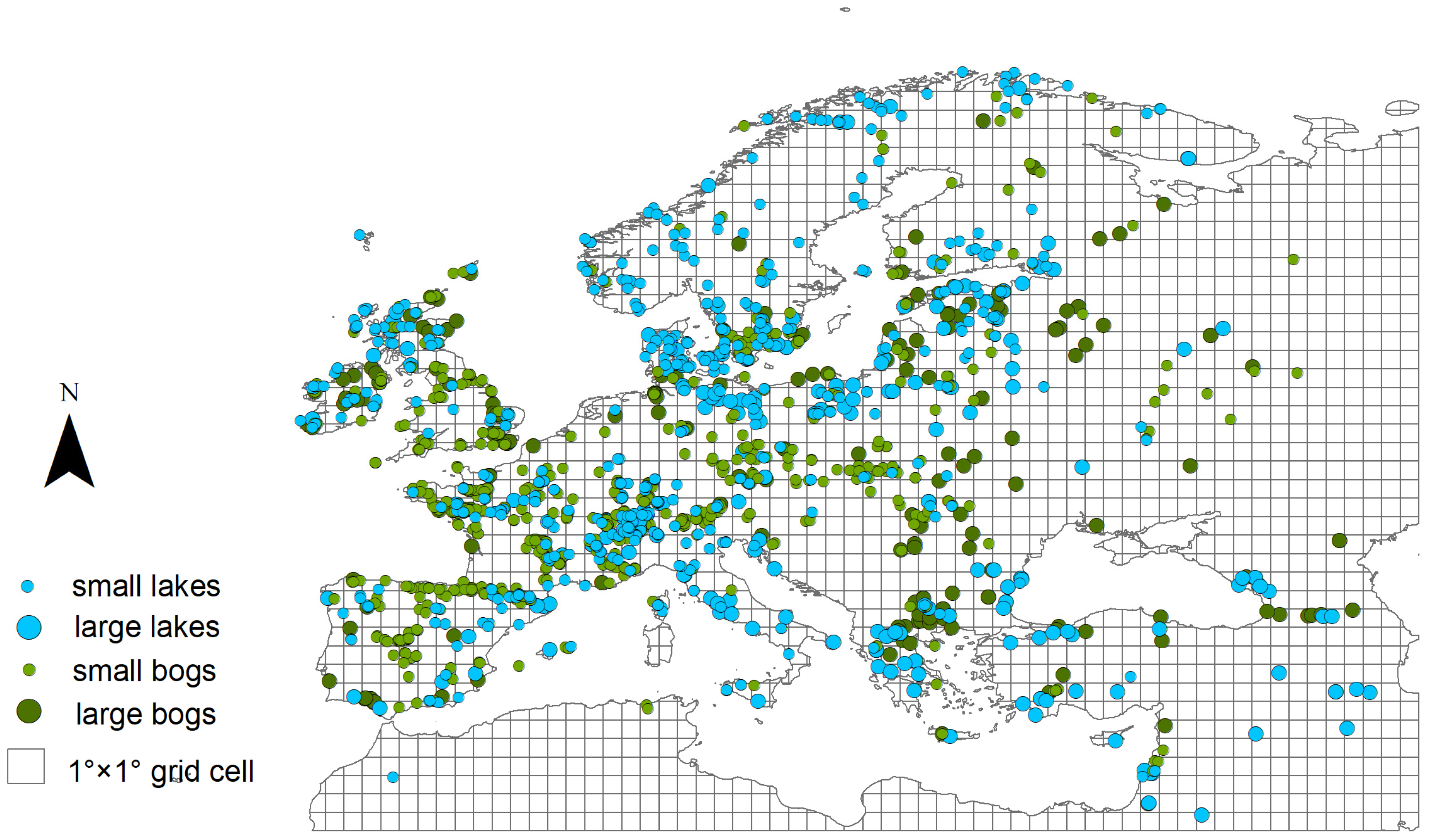
2.2. Fossil Pollen Records: Data Compilation and Preparation

A total of 1607 pollen records (923 and 684 sites from bogs and lakes, respectively) (see TERRANOVA_metadata in https://doi.org/10.48579/PRO/J5GZUO, accessed on 24 April 2023) was compiled from 41 countries covering all European countries, the western part of Russia and the eastern Mediterranean–Black Sea–Caspian corridor (Appendix A, Figure A1). This work benefited from earlier efforts and projects (Landclim I and II), which compiled pollen datasets from open-access databases and individual data contributors [31,33]. The Landclim II pollen dataset includes pollen data from the European Pollen Database [50,51], the Alpine Palynological Database (ALPADABA; Institute of Plant Sciences, University of Bern), the Czech Quaternary Palynological Database (PALYCZ; [52]), the Pyrenean Paleoenvironmental Database (PALEOPYR; [53]), and datasets compiled within synthesis projects from the Mediterranean region [7,11] and the eastern Mediterranean–Black Sea–Caspian corridor (EMBSeCBIO project; [54]). Most of the cited datasets are now archived in NEOTOMA [55]. The 479 new records that have been used here are either datasets added to Neotoma or the EPD until end of 2020 or collated from individual data contributors that fulfill the protocols applied in the Landclim projects. Pollen records are from natural terrestrial basins (lakes or bogs) with calibrated chronologies based on ≥3 dates. Where necessary new age-depth models expressed as (calibrated) calendar years before the present (i.e., cal BP = before 1950 CE, hereafter referred to as BP) were established in collaboration with the data contributors or database managers using the R-package clam [56].

Site radius information was obtained from original publications where possible. Where a site’s radius could not be determined from publication, it was geolocated in Google Earth, and the area of the site was measured. A radius value was extracted, assuming that a site shape is circular [28]. Available pollen records were filtered based on criteria including basin type (to exclude archaeological sites and marine records) and quality of chronological control (excluding sites with poor age-depth models or fewer than three radiocarbon dates).

Pollen counts were aggregated into 25 time windows across the Holocene (present–11,700 BP). The use of consecutive 500-year-long time windows results in REVEALS reconstructions with low SEs. The 500-year-long time windows are meaningful for the study of past land-cover changes over several millennia [31,34] and maximize the pollen-count size within time windows. This minimizes standard errors by decreasing variability between samples. Because human-induced land-cover changes were often more rapid since the early Middle Ages than through the earlier millennia, the three most recent time windows were fixed to present–100 BP (where the present is the year of coring), 100–350 BP, and 350–700 BP. An additional modern window was considered to evaluate the performance of the quality of the REVEALS reconstruction (see Section 2.3).

The taxonomy of each of the 1607 original pollen data files was harmonized. Pollen morphological types were assigned to 31 and 46 taxa (

Table 1. Land-cover types (LCTs) and their corresponding pollen morphological types. Fall speed of pollen (FSP) and the mean relative pollen productivity estimates (RPPs) for three different RPP-means datasets (RPPs.sts), with their standard deviations (SDs) in brackets (see text for more explanations). We highlighted the values that remain fixed across the RPPs.sts in green, the additional values considered in RPPs.st3 in blue and, the 15 additional RPP values (mostly entomophilous taxa) in RPPs.st2 in orange. For more information on species involved in the calculation of original RPP values, see Appendix B, Table A1.

Land Cover Types (LCTs)	Plant Taxa/Pollen-Morphological Types	FSP (m/s)	RPPs.st1 (SD)	RPPs.st2 (SD)	RPPs.st3 (SD)
Evergreen Trees (ET)	Abies	0.12	6.88(1.44)	6.88(1.44)	6.88(1.44)
	Buxus sempervirens	0.032	1.89(0.068)	1.89(0.068)	1.89(0.068)
	Empetrum	0.038		0.11(0.03)
	Ericaceae	0.038	4.27(0.094)	4.27(0.094)	0.07 (0.04)
	Juniperus	0.016	2.07(0.04)	2.07(0.04)	2.07(0.04)
	Phillyrea	0.015	0.51(0.075)	0.51(0.075)	0.51(0.075)
	Picea	0.056	5.44(0.10)	5.44(0.10)	2.62 (0.12)
	Pinus	0.031	6.06(0.24)	6.06(0.24)	6.38 (0.45)
	Pistacia	0.03	0.76(0.201)	0.76(0.201)	0.76(0.201)
	evergreen Quercus t.	0.035	11.04(0.261)	11.04(0.261)	11.04(0.261)
Summergreen Trees (ST)	Acer	0.056		0.63(0.156)
	Alnus	0.021	13.56(0.29)	13.56(0.29)	9.07 (0.10)
	Betula	0.024	5.11(0.30)	5.11(0.30)	3.09 (0.27)
	Carpinus betulus	0.042	4.52(0.43)	4.52(0.43)	3.55 (0.43)
	Carpinus orientalis	0.042	0.24(0.07)	0.24(0.07)	0.24(0.07)
	Castanea sativa	0.01	3.26(0.059)	3.26(0.059)	3.26(0.059)
	Corylus avellana	0.025	1.71(0.10)	1.71(0.10)	1.99 (0.20)
	Fagus	0.057	5.86(0.18)	5.86(0.18)	2.35 (0.11)
	Fraxinus	0.022	1.04(0.05)	1.04(0.05)	1.03 (0.11)
	Populus	0.025		2.66(1.25)
	deciduous Quercus t.	0.035	4.54(0.09)	4.54(0.09)	5.83 (0.15)
	Salix	0.022	1.18(0.08)	1.18(0.08)	1.22 (0.11)
	Sambucus nigra t.	0.013		1.30(0.12)
	Tilia	0.032	1.21(0.12)	1.21(0.12)	0.80 (0.03)
	Ulmus	0.032	1.27(0.05)	1.27(0.05)	1.27(0.05)
Open Land (OL)	Amaranthaceae/Chenopodiaceae	0.019	4.28(0.270)	4.28(0.270)	4.28(0.270)
	Apiaceae	0.042		3.09(0.615)
	Artemisia	0.025	3.94(0.15)	3.94(0.15)	3.48 (0.20)
	Calluna vulgaris	0.038	1.09(0.03)	1.09(0.03)	0.82 (0.02)
	Cerealia t.	0.06	1.85(0.38)	1.85(0.38)	1.85 (0.38)
	Comp. SF. Cichorioideae	0.051		0.36(0.137)
	Cyperaceae	0.035	0.96(0.05)	0.96(0.05)	0.87 (0.06)
	Fabaceae	0.021		0.4(0.07)
	Filipendula	0.006	3.00(0.28)	3.00(0.28)	2.81 (0.43)
	Comp. Leucanthemum (Anthemis) t.	0.029		0.10(0.008)
	Plantago lanceolata	0.029	2.33(0.20)	2.33(0.20)	1.04 (0.09)
	Plantago media	0.024		1.27(0.18)
	Plantago montana	0.03		0.74(0.13)
	Poaceae	0.035	1.00 (0.00)	1.00 (0.00)	1.00 (0.00)
	Potentilla t.	0.018		1.19(0.133)
	Ranunculus acris t.	0.014		1.99(0.265)
	Rubiaceae	0.019		3.95(0.314)
	Rumex acetosa t.	0.018	3.02(0.28)	3.02(0.28)	2.14 (0.28)
	Secale cereale	0.06	3.99(0.32)	3.99(0.32)	3.02 (0.05)
	Trollius	0.013		2.29(0.36)
	Urtica	0.007		10.52(0.31)
	Number of taxa		31	46	31

) using an updated dictionary table from [31] following the protocol described in [33]. Samples from each harmonized record were aggregated in time windows using the assigned calibrated ages BP from each age-depth model. The pollen records were then filtered to remove time windows with fewer than 100 pollen grains to avoid sterile samples that would compromise the correctness of the REVEALS estimates.

RPP (relative to Poaceae, RPP = 1) is one of the most important input parameters required to run the REVEALS model [27]. We test the inclusion or exclusion of plant taxa with dominant entomophily and the effect of RPP values on the grid-based REVEALS estimates (Gb-RVest). The selection of RPP studies, RPP values, and calculation of mean RPP and their standard deviation (SD) for Europe (Table 1) are explained in Appendix B,

Table A1. Available RPPs values for the selected taxa used to calculate the RPPs-means and their SDs of the 31 and 46 taxa in the datasets (i.e., RPPs.st1, RPPs.st2, RPPs.st3). RPPs (with their standard deviations SDs) of 26 tree pollen taxa and 23 herbs, and small shrubs in 17 study areas. The type of surface samples and the ERV submodel used to calculate the original RPPs are indicated. The superscript numbers 1, 2, 3 indicate the values that were not included in the RPPs.st1, st2, and st3, respectively. If no superscript number, the value is included in all three datasets. Poaceae was selected as reference taxon. * RPPs from Germany [68], reference taxon Pinus. RPPs converted to Poaceae as reference taxon. The RPP estimates selected in this case were obtained with a vegetation dataset including only the trees that had reached their flowering age. ** RPPs from Germany [95]; in the original publication, the ERV analysis was performed with the Lagrangian stochastic model (LSM) for the dispersal of pollen and with Pinus as a reference taxon. In Githumbi et al. (2022), Martin Theuerkauf redid the analysis with the Gaussian Plume model for the dispersal of pollen [45,90] and with Poaceae as a reference taxon.

	Moss Polster Sites Used to Calculate RPPs								Lake Sites Used to Calculate RPPs
Region	Finland [89]	C Sweden [75]	S Sweden [98,99]	Norway [96]	England [91]	Swiss Jura [100]	C Bohemia (Czech Rep.) [92]	Bialowieza Forest (Poland) [97]	Estonia [94]	Denmark [93]	Swiss Plateau [101]	Germany * [68]	Germany ** [95]	France Mediterranean [31]	Romania [87]
ERV submodel	ERV 3	ERV 3	ERV 3	ERV 1	ERV 1	ERV 1	ERV 1	ERV 3	ERV 3	ERV 1	ERV 3	ERV 3		ERV	ERV
Poaceae (Reference taxa)	1.00 (0.00)	1.00 (0.00)	1.00 (0.00)	1.00 (0.00)	1.00 (0.00)	1.00 (0.00)	1.00 (0.00)	1.00 (0.00)	1.00 (0.00)	1.00 (0.00)	1.00 (0.00)	1.00 (0.00)	1.00 (0.00)	1.00 (0.00)	1.00 (0.00)
Herb taxa
Amaranthaceae/Chenopodiaceae (mainly Amaranthus retroflexus and Chenopodium album)							4.28 (0.27)
Apiaceae				0.26 (0.009) 1,3											5.91 (1.23) 1,3
Artemisia (mainly A. vulgaris)							2.77 (0.39) 3		3.48 (0.20) 1,2				5.56 (0.020) 3		5.89 (3.16) 1,2,3
Calluna vulgaris		0.30 (0.03) 1,2	4.70 (0.69) 1,2,3	1.07 (0.03)						1.10 (0.05)
Cerealia t. (Secale and Zea excluded except in Grindean et al. 2019)			3.20 (1.14)				0.0462 (0.0018) 1,2,3		1.60 (0.07)	0.75 (0.04)	0.00076 (0.0019) 1,2,3	9.00 (1.92) 1,2,3	0.08 (0.001) 1,2,3		0.22 (0.12) 1,2,3
Comp. SF. Cichorioideae (Comp SF Asteroideae excluded except in Grindean et al. 2019)			0.24 (0.06) 1,3	0.06 (0.004) 1,3							0.17 (0.03) 1,3			1.161 (0.675) 1,3	0.16 (0.1) 1,3
Comp. Leucanthemum (Anthemis) t. (Achillea millefolium and Leucanthemum vulgare)				0.10 (0.008) 1,3
Cyperaceae	0.002 (0.0022) 1,2,3	0.89 (0.03)	1.00 (0.16)	0.29 (0.01) 1,2,3		0.73 (0.08)			1.23 (0.09) 3
Empetrum (mainly E. nigrum subsp. hermaphroditum)	0.07 (0.06) 1,2,3	0.11 (0.03) 1,3
Ericaceae (Calluna excluded, Vaccinium spp. dominant in NE and Arbutus unedo and Erica arborea dominant in SE)		0.07 (0.04) 1,2												4.265 (0.094) 3
Filipendula (F. ulmaria)			2.48 (0.82)	3.39 (missing, 0.00) 3					3.13 (0.24)
Plantago lanceolata			12.76 (1.83) 1,2,3	1.99 (0.04)			3.70 (0.77) 3			0.90 (0.23)	0.24 (0.15) 1,2		2.73 (0.043) 3		0.58 (0.32) 1,2,3
Plantago media						1.27 (0.18) 1,3
Plantago montana (Plantago atrata)						0.74 (0.13) 1,3
Potentilla t. (Potentilla spp. dominant)			2.47 (0.38) 1,3	0.14 (0.005) 1,3		0.96 (0.13) 1,3
Ranunculus acris t. (R. acris, R. repens, Clematis flammula, C. vitalba)			3.85 (0.72) 1,3	0.07 (0.004) 1,3										2.037 (0.335) 1,3
Rubiaceae (Galium spp. dominant)			3.95 (0.59) 1,3	0.42 (0.01) 1,3		3.47 (0.35) 1,3									7.97 (1.08) 1,3
Rumex acetosa t. (mainly R. acetosa and R. acetosella)			4.74 (0.83)	0.13 (0.004) 1,2						1.56 (0.09)			2.76 (0.022) 3
Secale cereale			3.02 (0.05)									4.08 (0.96) 3	4.87 (0.006) 3
Trollius (Trollius europaeus)						2.29 (0.36) 1,3
Urtica (mainly U. dioica)							10.52 (0.31) 1,3
Vaccinium (Vaccinum spp.)	0.01 (0.01) 1,2,3
Tree taxa
Abies (A. alba)						3.83 (0.37)					9.92 (2.86)
Acer (A. spp., A. platanoides, A. pseudoplatanus, A. tataricum)			1.27 (0.45) 1,3			0.32 (0.10) 1,3									0.3 (0.09) 1,3
Alnus (A. spp.)			4.20 (0.14) 1,2		8.74 (0.35)		2.56 (0.32) 1,2,3	15.95 (0.6622) 3	13.93 (0.15)			15.51 (1.25) 3	13.68 (0.049) 3
Betula (mainly B. pubescens, B. pendula)	4.6 (0.70)	2.24 (0.20)	8.87 (0.13) 3		6.18 (0.35)			13.94 (0.2293) 1,2,3	1.81 (0.02) 3		2.42 (0.39)	9.62 (1.92) 3	19.70 (0.117) 1,2,3
Buxus sempervirens														1.89 (0.068)
Carpinus betulus			2.53 (0.07) 1,2					4.48 (0.0301) 3			4.56 (0.85)	9.45 (0.51) 1,2,3
Carpinus orientalis															0.24 (0.07)
Castanea sativa														3.258 (0.059)
Corylus avellana			1.40 (0.04)		1.51 (0.06)			1.35 (0.0512) 3			2.58 (0.39)			3.44 (0.89) 1,2,3
Cupressaceae (Juniperus communis, J. phoenicea, J. oxycedrus)														1.618 (0.16) 1,2,3
Deciduous Quercus t. (Q. spp., Q. petrae, Q. rubra, Q. cerris, Q. pubescens)			7.53 (0.08)		5.83 (0.00)		1.76 (0.20) 3	18.47 (0.1032) 1,2,3	7.39 (0.20)		2.56 (0.39)	2.15 (0.17) 3	17.85 (0.049) 1,2,3		1.10 (0.35) 1,2,3
Evergreen Quercus t. (Q. ilex, Q. coccifera)														11.043 (0.261)
Fabaceae															0.4 (0.07) 1,3
Fagus (F. sylvatica)			6.67 (0.17) 3			1.20 (0.16) 1,2				5.09 (0.22)	0.76 (0.17) 1,2	5.83 (0.45) 3	9.63 (0.008) 1,2,3
Fraxinus (F. excelsior in NE, F. excelsior and F. ornus in SE)			0.67 (0.03)		0.70 (0.06) 3		1.11 (0.09) 3				1.39 (0.21)	6.74 (0.68) 1,2,3	1.35 (0.012) 3		2.99 (0.88) 1,2,3
Juniperus (J. communis)		0.11 (0.45) 1,2,3	2.07 (0.04)
Larix/Pseudotsuga												8.77 (1.81) 1,2,3
Phillyrea (P. angustifolia, P. latifolia, P. media)														0.512 (0.075)
Picea (mainly P. abies)		2.78 (0.21)	1.76 (missing, 0.00) 1,2			8.43 (0.30) 3			4.73 (0.13)	1.19 (0.42) 1,2	0.57 (0.16) 1,2,3	1.58 (0.28) 1,2,3	5.81 (0.007) 3
Pinus (mainly P. sylvestris)	8.40 (1.34)	21.58 (2.87) 1,2,3	5.66 (missing, 0.00)				6.17 (0.41) 3	23.12 (0.2388) 1,2,3	5.07 (0.06)		1.35 (0.45) 1,2,3	5.66 (0.00) 3	5.39 (0.222) 3
Pistacia (P. lentiscus, P. therebinthus)														0.755 (0.201)
Populus (P. alba)												2.66 (1.25) 1,3
Salix (S. spp.)		0.09 (0.03)	1.27 (0.31)		1.05 (0.17)		1.19 (0.12) 3		2.31 (0.08)
Sambucus nigra t. (mainly S. nigra)							1.30 (0.12) 1,3
Tilia (mainly T. cordata)			0.80 (0.03)				1.36 (0.26) 3	0.98 (0.0263) 1,2,3				1.47 (0.23) 3	12.38 (0.101) 1,2,3
Ulmus (mainly U. glabra)			1.27 (0.05)										11.51 (0.101) 1,2,3
Number of taxa	5	9	25	11	6	10	11	7	10	6	12	13	14	10	11

. This paper uses three alternative RPP-means datasets (Table 1) to evaluate the effect of RPP selection on REVEALS results.

RPPs.st1 (31 taxa) is the European RPP-means dataset from [31]. It includes plant taxa from boreal, temperate, and Mediterranean Europe for the calculation of the RPP-mean values. In this selection, most entomophilous herbs are excluded, except the most common taxa with mixed wind and insect transport, such as Amaranthaceae/Chenopodiaceae, Fi—lipendula, Rumex acetosa t., and Plantago lanceolata. Note that the entomophilous tree Tilia and partly entomophilous tree/shrub Salix are included.

RPPs.st2 (46 taxa) is a new synthesis proposed in this study, inclusive of a larger number of entomophilous taxa. It uses the same 31 taxa and mean values of RPP used in the first dataset [31] and 13 additional entomophilous taxa (some with mixed wind and insect transport), i.e., Empetrum, Acer, Sambucus nigra t., Fabaceae, Apiaceae, Compositae SF. Cichorioideae, Comp. Leucanthemum (Anthemis) t., Plantago media, Plantago montana, Ranunculus acris t., Potentilla t., Rubiaceae, and Trollius, as well as Populus and Urtica (mainly anemophilous). For these additional taxa, the mean was calculated using all available European RPP values (Appendix B, Table A1) based on standard 2 from [28]. We excluded values that were not significantly different from zero considering the lower bound of its SD (e.g., Empetrum, 0.07) and values assumed to be outliers or unreliable in the original publications. The RPPs.st2 is used to test the sensitivity of the REVEALS model to the use of pollen types from entomophilous plant taxa, although the model assumes that all pollen is transported by wind (see Section 2.1).

RPPs.st3 (31 taxa) is a composed dataset that compiled 24 plant taxa and their RPP values selected by [28,33] and 7 Mediterranean plant taxa: Amaranthaceae/Chenopodiaceae, Buxus sempervirens, Carpinus orientalis, Castanea sativa, Phillyrea and evergreen Quercus t. [31]. RPPs.st3 differs from RPPs.st2 and RPPs.st1 for 19 RPPs values of the following taxa: Picea, Pinus, Ericaceae, Betula, Corylus avellana, Fraxinus, deciduous Quercus t., Carpinus betulus, Fagus, Tilia, Salix, Calluna vulgaris, Artemisia, Cyperaceae, Filipendula, Plantago lanceolata, Rumex acetosa t., and Secale cereale. The following 12 plant taxa share the same mean value of RPP for all three datasets: Abies, Juniperus, Phillyrea, Pistacia, evergreen Quercus t., Buxus sempervirens, Carpinus orientalis, Castanea sativa, Ulmus, Amaranthaceae/Chenopodiaceae, Poaceae, and Cerealia t.

Fall speed of pollen (FSP) values are listed in [31].

2.3. Modern Vegetation and Pollen Datasets

To perform an evaluation of the quality of the REVEALS results and the effect of RPP-means datasets (RPPs.st1, RPPs.st2, and RPPs.st3) on the grid-based REVEALS estimates (Gb-RVest), we compared the sum of REVEALS-based tree cover for the most recent decades (RV-Trees) with modern measurements of tree cover (GFC-Trees).

GFC-Trees was derived from the global forest change dataset [57]. This is based on the analysis of Landsat 7 Enhanced Thematic Mapper Plus data at a 30-m spatial resolution to characterize forest extent, loss, and gain from 2000 to 2012. We used tree cover data for the year 2000 that expresses tree cover (defined as vegetation taller than 5 m in height) as a percentage per output grid cell. All forms of natural forests or plantations across a range of canopy densities are considered. Broadleaved and coniferous trees are not differentiated. Original tree cover data are viewable and downable at full resolution at http://earthenginepartners.appspot.com/science-2013-global-forest, accessed on 21 March 2023.

RV-Trees values are based on the Gb-RVest results from the core top samples (−45 to −55 BP, i.e., 1995 AD to 2005 AD). GB-RVest results for taxa in the summer green trees and evergreen tree groups (Table 1) have been summed. The number of core top records from large lakes is limited in Europe (N = 9), and thus we have included Gb-RVest, which is based on multiple small-sized sites within our evaluation of RPP-mean datasets. The total number of grid cells used is 111. This results in 36 grid cells with lakes and 75 grid cells with both lakes and bogs (of which 47 with only ≥1 bog(s)) of all radii. Therefore, the modern pollen dataset covered 20 European countries from the Mediterranean to the boreal vegetation zones, with a tree-cover gradient from 1% to 80% (Figure 2). The same pollen dataset was used for the comparison between raw pollen data (RW-data) and GFC-Trees for 31 taxa and 46 taxa.

Comparison of RV-Trees with GFC-Trees required a transformation of the spatial resolution of the modern tree cover. While the tree cover is available at 1 arc-minute resolution, the REVEALS reconstructions were prepared for 1° grid cells. We aggregated the tree-cover data to the REVEALS grid by averaging the tree-cover percentages in each REVEALS grid cell (Figure 2).

2.4. REVEALS Run and Data Analysis

The REVEALS function within the LRA R-package [58] was used to produce grid-based REVEALS estimates (Gb-RVest). In this study, we selected the Gaussian Plume model to describe pollen dispersal as selected RPP values are derived from the GPM model. Depending on the type of site, the REVEALS function used a different deposition model, Sugita’s model for lakes and ponds [40] or Prentice’s model for bogs and mires [43,44]. Pollen records from all sites, regardless of their size, are used to maximize the number of pollen records within each 1° × 1° grid cell across the studied area. For the grid cells that include pollen data from both lakes and bogs, we apply REVEALS separately for the lake and bog data and then combine results to produce a single mean Gb-RVest and its standard error (SE) for each taxon.

When running REVEALS, neutral atmospheric conditions and wind speed of 3 m.s⁻¹ as in [27,28,31,33] are assumed. Z_max, the maximum spatial extent of the regional vegetation from the centre of the site, is set to 50 km, roughly corresponding to a 1° × 1° grid cell [28,31,33].

REVEALS results are extracted by time window, producing 25 matrices of mean Gb-RVest and 25 matrices of corresponding mean SEs for each of the RPP taxa and each grid cell. As three RPP-means datasets are tested, three REVEALS results are produced per time window. The taxon-based Gb-RVest are then grouped into land-cover types (LCTs, Table 1), hereafter named Gb-RVest-LCTs. For the modern time window (−45 to −55 BP), as the RV-Trees do not separate the contributions of evergreen and summer green species, the sum of the two Gb-RVest-LCTs was calculated for comparison with GFC-Trees (Table 1). The SEs of each Gb-RVest-LCT and overall tree cover were calculated using the delta method [59].

We use here major axis (MA) as the regression method (see Appendix C) [60,61] to explore the bivariate relationships between two pairs of variables, or data series: among different RPPs.sts over the Holocene (RPPs.st2 vs. RPPs.st1 and RPPs.st3 vs. RPPs.st1) and between modern vegetation and REVEALS results.

Further, pairs of Gb-RVest-LCTs (RPPs.st1 vs. RPPs.st2, RPPs.st1 vs. RPPs.st3) for all time windows together were compared calculating the difference between the values in each grid cell, geolocalizing in the map of Europe the negative and positive values.

3. Results

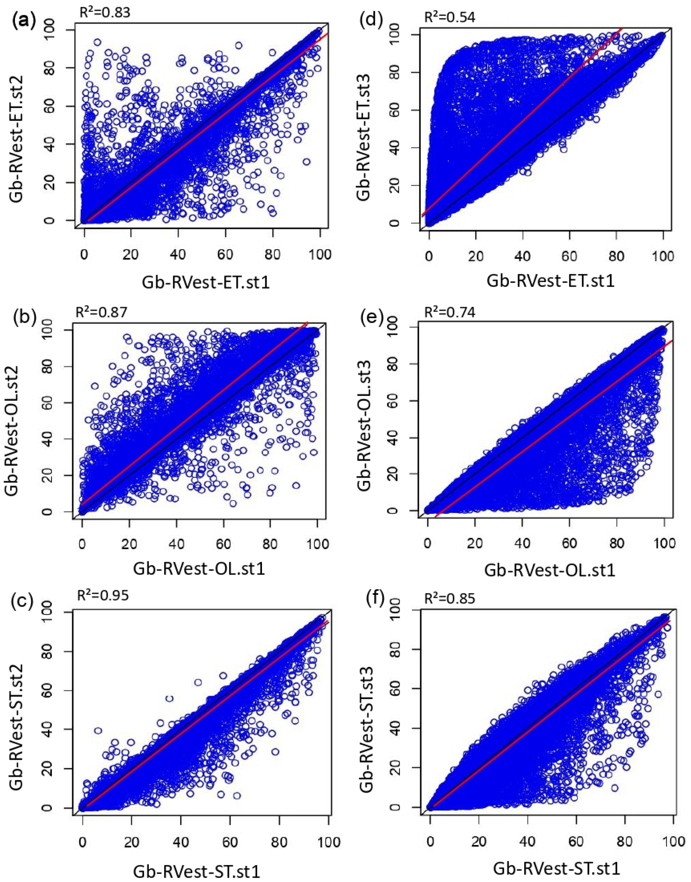
3.1. Effect of Type and Number of Pollen Taxa in RPP-Means Datasets on Gb-RVest-LCTs

In this section, we evaluate how Gb-RVest-LCTs, using RPPs.st1 as a reference, compare to RPPs.st2 and RPPs.st3 (Figure 3) and formulate hypotheses on the nature of these relationships and how they vary across RPP-means datasets.

The strongest association in the MA regression results is between Gb-RVest.st1 and Gb-RVest.st2, with R² values of 0.834 (ET), 0.876 (OL), and 0.953 for (ST). The R² values of the comparison between Gb-RVest.st1 and Gb-RVest.st3 are 0.569 (ET), 0.784 (OL), and 0.858 (ST). ET-RV.st2 values are generally lower than ET-RV.st1 (r = −0.109), as are OL-RV.st3 compared to OL-RV.st1 (r = −0.094), ST-RV.st2 compared to ST-RV.st1 (r = −0.134), and ST-RV.st3 compared to ST-RV.st1 (r = −0.031). ET-RV.st3 values are generally higher than ET-RV.st1 (r = 0.242), as are OL-RV.st2 compared to OL-RV.st1 (r = 0.104) (values of r not shown in Figure 3).

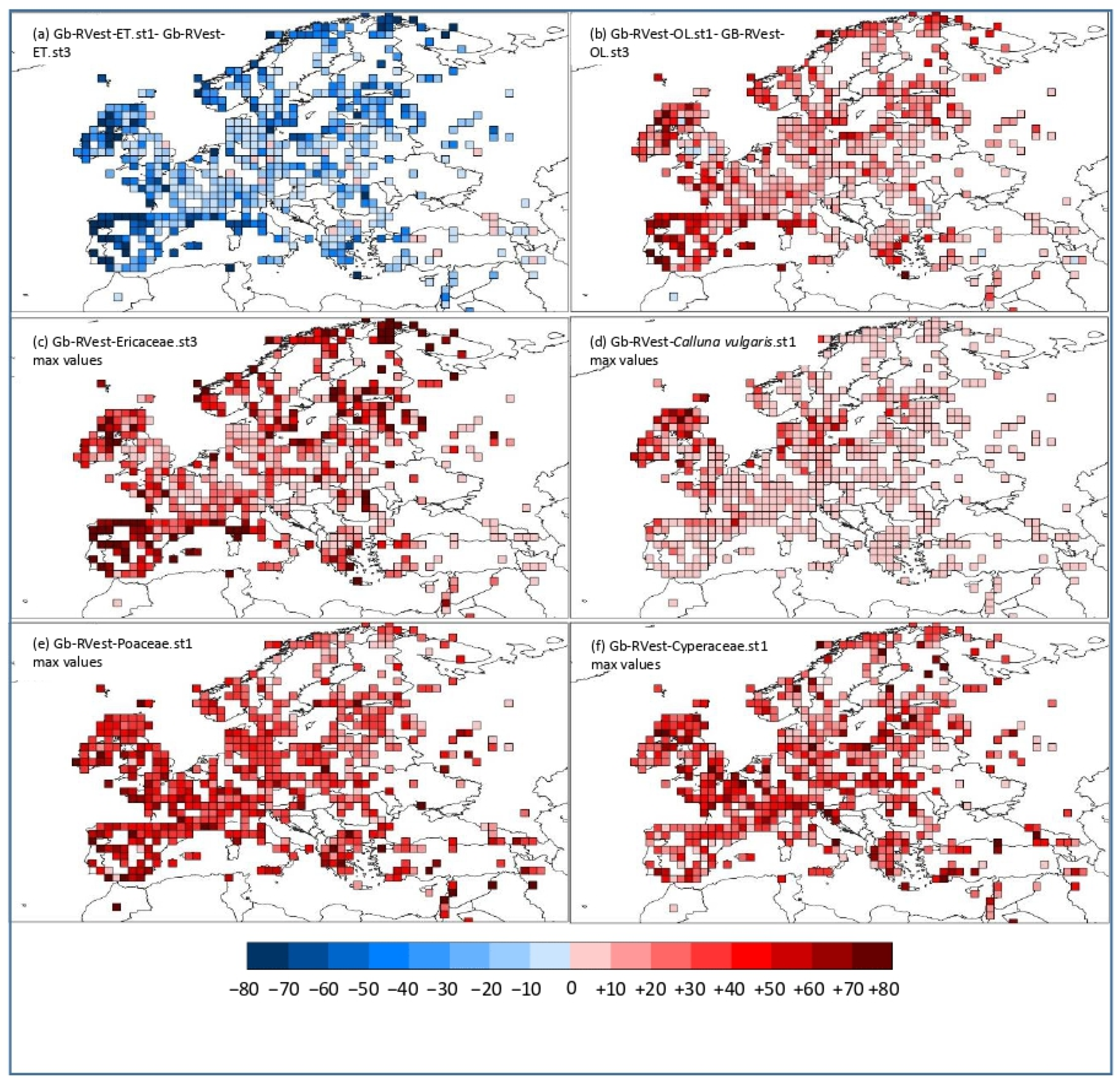
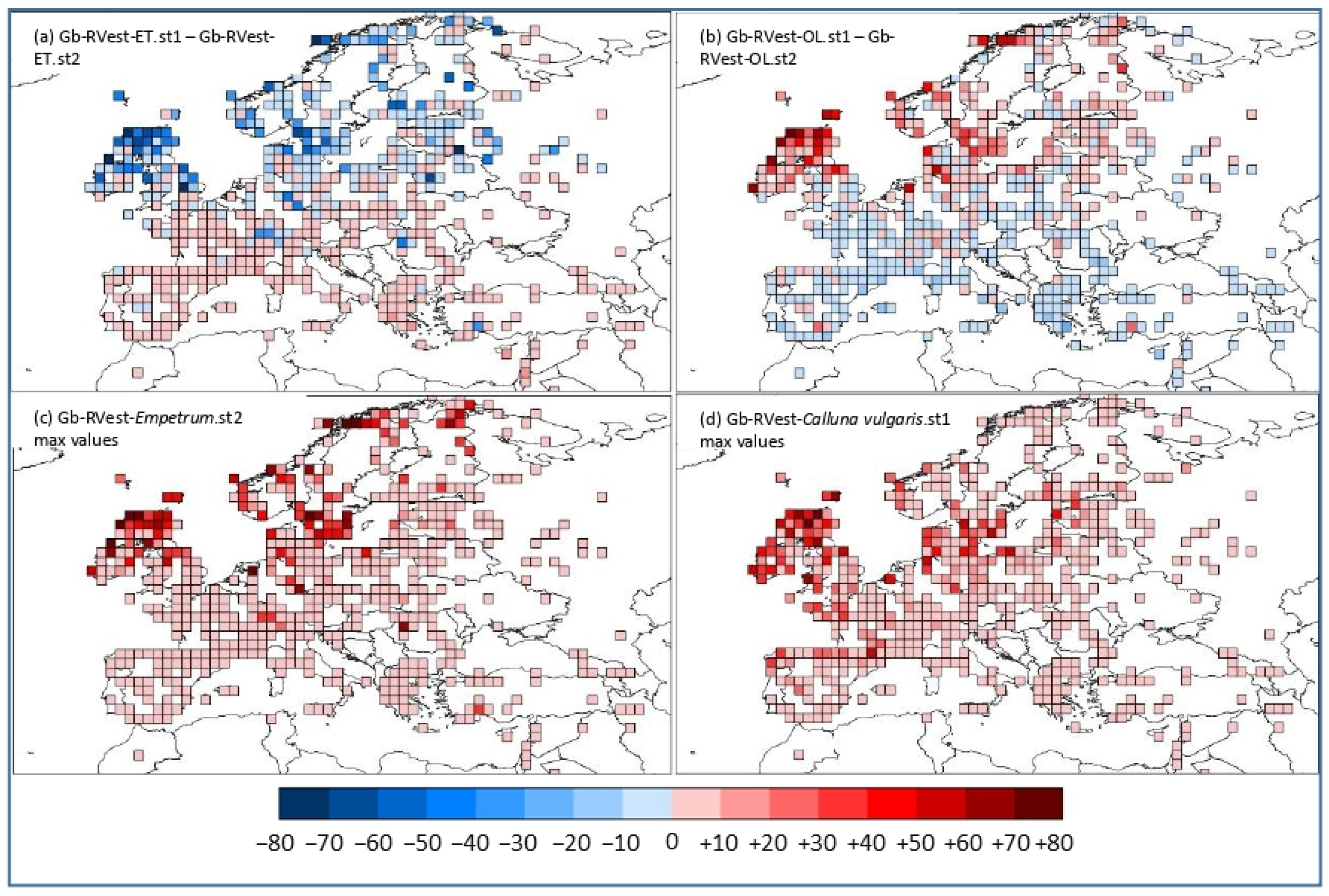
3.2. Geographical Pattern of the Gb-RVest-LCTs Differences between RPP-Means Datasets

Differences between pairs of Gb-RVest-LCTs were mapped using the positive and negative results of the differences (i.e., diff.A, Figure 4a,b; diff.B, Figure 5a,b). Furthermore, the negative and positive values of the differences are explain by maximum values of the most representative taxa over all time windows (Figure 4c–f and Figure 5c,d). These taxa influence the over- or under-representation of LCT in the analyses.

The greatest differences between Gb-RVest-LCTs.st1 and Gb-RVest-LCTs.st3 (diff.A) (Figure 4a,b) are found within ET and OL. ST values are broadly comparable. The greatest differences between Gb-RVest-ET.st3 and Gb-RVest-ET.st1 are located in Spain, Portugal, southern France, central Italy, and the U.K. (Figure 4a). Ericaceae appears to be the taxon that causes this overrepresentation of Gb-RVest-ET.st3 in comparison to Gb-RVest-ET.st1 (Figure 4c). Lower values of ET in Gb-RVest.st1 are compensated by Calluna vulgaris, Cyperaceae, and Poaceae (Figure 4d–f).

The greatest differences between Gb-RVest-LCTs.st1 and Gb-RVest-LCTs.st2 are found within ET and OL (diff.B) (Figure 5a,b). The greatest differences are found within the U.K., Ireland, southern Sweden, and scattered grid cells from central to Eastern Europe. Empetrum causes the overrepresentation of Gb-RVest-ET.st2 in comparison to Gb-RVest-ET.st1 (Figure 5c). Lower values of Gb-RVest-ET.st1 are compensated by OL (Figure 5b), in particular Calluna vulgaris (Figure 5d).

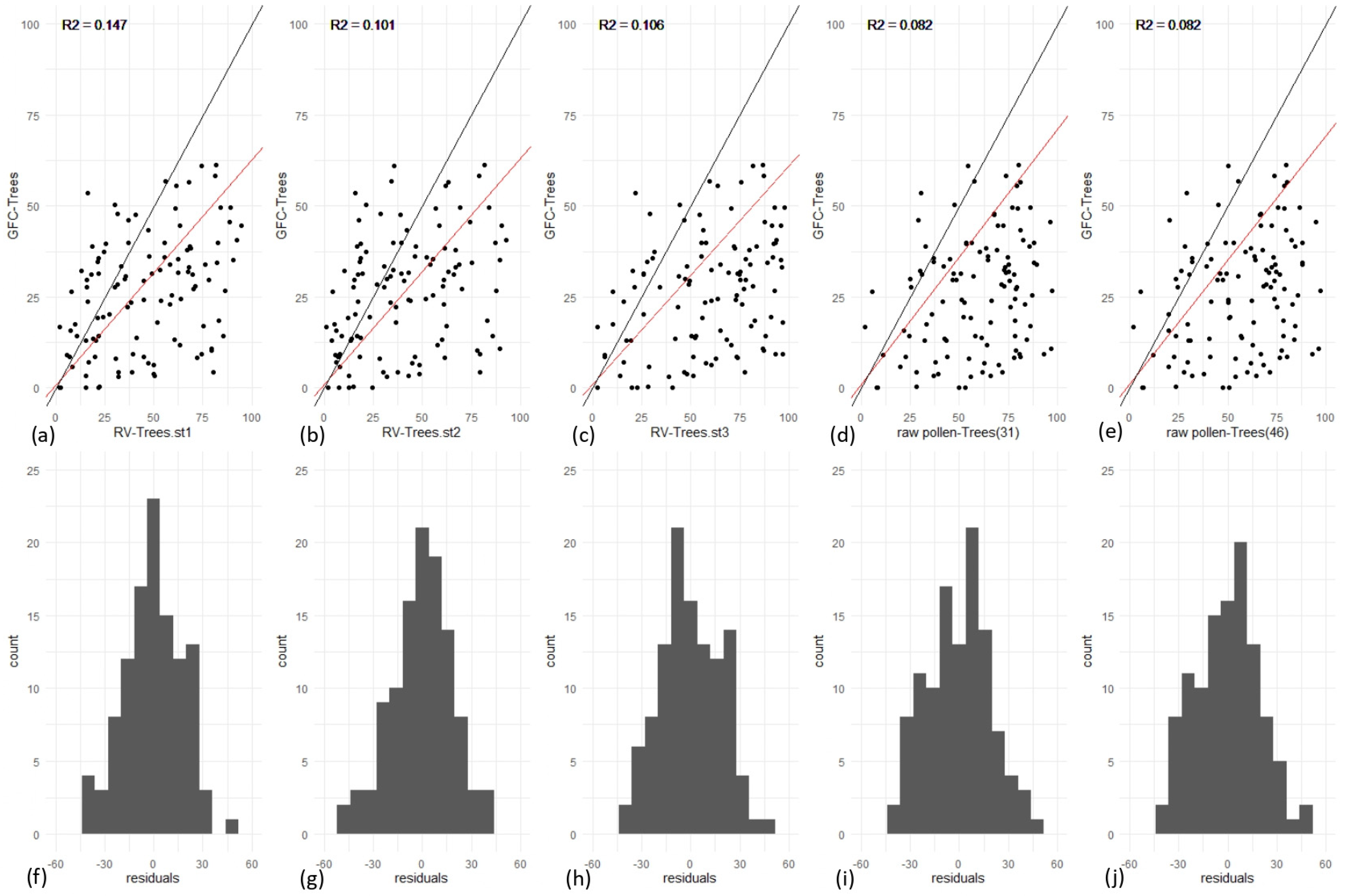
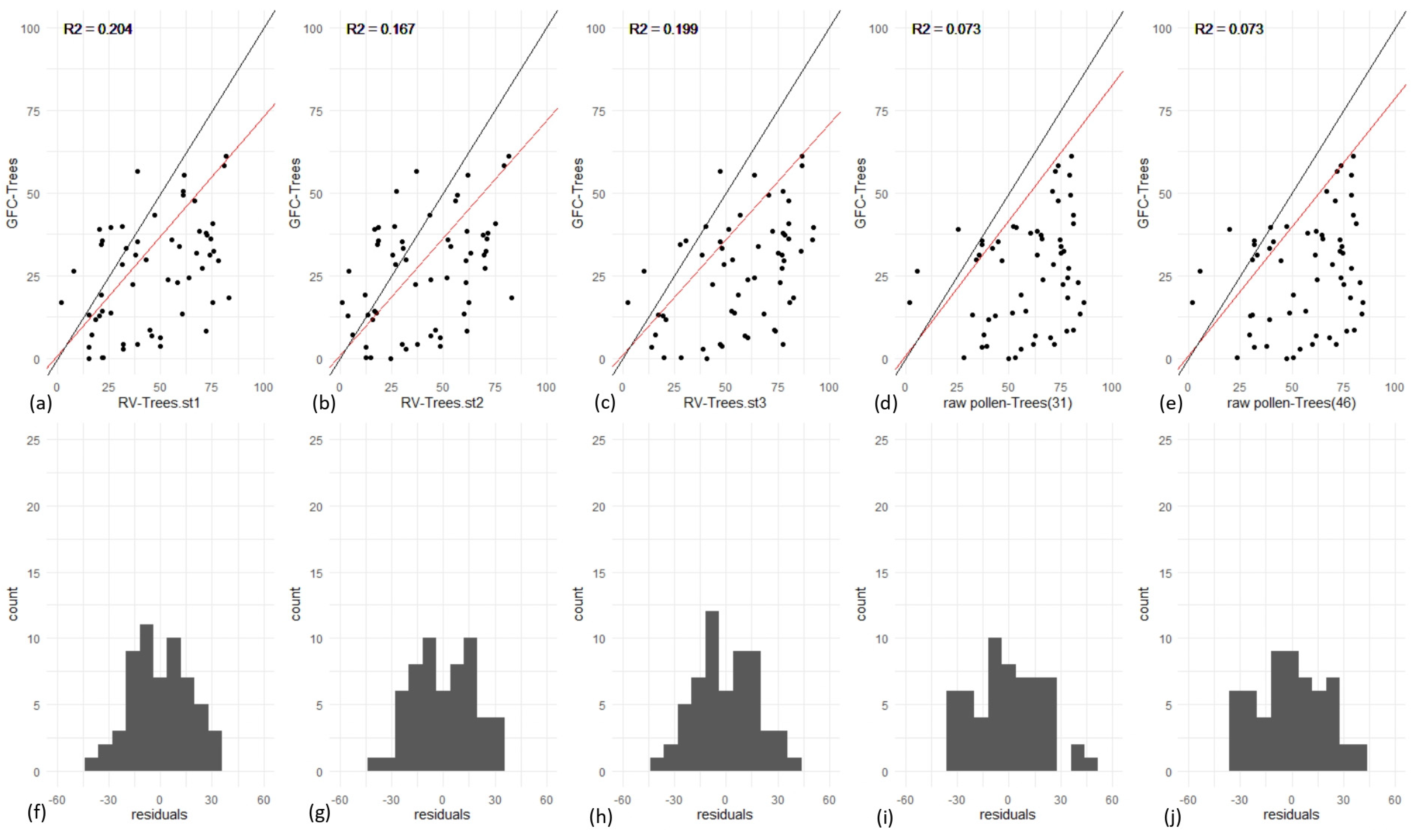
3.3. REVEALS Validation for All Europe

Validation was undertaken on two groups of sites (lakes only: RV-Trees.L.st1; lakes plus bogs: RV-Trees.LnB.st1) to test (a) which RPPs.sts to use in the REVEALS model in order to have robust reconstructions on a wide scale, and (b) whether the inclusion of bog sites influences the goodness of fit between REVEALS model results and modern vegetation.

Comparing the slope values obtained by MA regression for both groups shows a greater association for GFC-Trees vs. RV-Trees.LnB.st1 (0.619) and GFC-Trees vs. RV-Trees.L.st1 (0.722) than in GFC-Trees vs. RV-Trees.LnB.st2 (0.600), GFC-Trees vs. RV-Trees.LnB.st3 (0.601), GFC-Trees vs. RV-Trees.L.st2 (0.709), and GFC-Trees vs. RV-Trees.L.st3 (0.698). RV-Trees.st1 is, therefore, statistically more similar to GFC-Trees than those obtained from the other two RPP sets (Figure 6 and Figure 7a–c). The R² values confirm this analysis. The strongest associations are GFC-Trees vs. RV-Trees.LnB.st1 (0.147) and GFC-Trees vs. RV-Trees.L.st1 (0.203) rather than in GFC-Trees vs. RV-Trees.LnB.st2 (0.105), GFC-Trees vs. RV-Trees.LnB.st3 (0.106), GFC-Trees vs. RV-Trees.L.st2 (0.167), or GFC-Trees vs. RV-Trees.L.st3 (0.199) (Figure 6 and Figure 7a–c).

The best-fit relationship in both MA regression analyses between GFC-Trees and RV-Trees.L.sts/RV-Trees.LnB.sts shows that trees are over-represented in the RV results (Figure 6 and Figure 7a–c). The residuals (Figure 6 and Figure 7f–h) are normally distributed across the RV-Trees gradient.

RW-data (for 31 and 46 taxa, for lakes, and lakes and bogs) was used instead of RVest, to test whether the use of raw pollen-Trees rather than RV-Trees better represented the actual forest cover (GFC-Trees) (Figure 6 and Figure 7d,e). The results show that raw pollen-Trees have a worse association with GFC-Trees than RV-Trees. The regression between raw pollen-Trees (31 and 46 taxa) for lakes and bogs and GFC-Trees only has a weak association (R² = 0.082) (Figure 6d,e), and for the lakes-only group, an even lower R² (0.073) (Figure 7d,e). The residuals in both cases are not normally distributed along the regression line (Figure 6 and Figure 7i,j).

4. Discussion

Our discussion focuses on (i) proposing a robust RPP-means dataset, through validation, for a reliable representation of vegetation for the last 11,700 years BP at a European scale, (ii) the influence of different RPP-means datasets on Gb-RVest as a test of the sensitivity of the REVEALS approach, (iii) the evaluation of some challenging taxa, and (iv) the importance of the number of pollen records for high-quality Gb-RVest to capture transient vegetation change at a sub-millennial time scale through the Holocene.

4.1. New Insight after Validation

Testing the reliability of REVEALS-based reconstructions relies on comparison with different datasets, such as remote sensing data, and here we have used the global forest change dataset (GFC). Neither RVest nor GFC provides a completely accurate reflection of the “actual” vegetation. Both are subject to a number of potential sources of errors, as already observed in [62] in the correspondence between CORINE [63] and pollen-based land-cover classes. This study shares some similar challenges for comparing estimates of vegetation based on the remotely sensed and pollen-inferred land cover with [62], which might have influenced the validation as a whole. These include: (1) georeferencing inaccuracies: misplaced pollen site locations can affect both GFC (by extracting the wrong forest cover data for sites) and RVest (by placing sites in the wrong grid cells); (2) misclassification of land cover as remote sensing techniques make it difficult to differentiate between land-cover types (e.g., the determination of different forest types) and not all land-cover types are detectable via remote sensing; (3) the normalization factor applied to both RVest and GFC to make the datasets comparable leads to loss of some details. However, our comparison differs from that of [62] for several reasons, which are: (1) the approach used to transform pollen data into records of land-cover change, as we have been able to compare quantified values in both RVest and GFC, rather than compare classification results (via biomization techniques used in [62]), (2) the modern vegetation used, (3) the use of modern surface pollen samples.

The global forest change dataset is >80% accurate [57]. It is the most widely used forest cover product for global and regional analyses due to its high resolution (30 m), standardized classes, yearly updates, and convenient and cost-free use [64]. It also has the advantage of being a time series of changes in tree cover [65]. Nevertheless, a number of sources of error are specific to GFC. In [65,66], accuracy issues for this dataset are reported. GFC is less accurate in mountainous regions due to a combination of intense cloudiness and topographic shadowing [67]. GFC is also unable to distinguish between natural forest cover and agricultural tree crops [66]. Lower accuracy is also reported in regions with sparse and variable tree cover due to the background signal or seasonal variability in phenology or cloud cover. Another limiting factor can be ascribed to the rescaling process that limits the ability of the dataset to capture tree canopy cover values on the ground at 30 × 30 m as it is derived from a coarser-resolution product [64].

In this study, the number of available modern pollen datasets with top cores samples was limited. For the sake of complete Europe-wide validation, as many sites (191) as possible were considered, including small lakes and bogs. A total of 41% of the grid cells (111 out of 539) had top core samples useful for comparison. Our comparison revealed that RPPs.st1 is the most suitable to represent modern vegetation in Europe, both using bogs and lakes, or only lakes, as suggested by [31]. The REVEALS model improved the accuracy of vegetation reconstruction significantly over the pollen proportions alone. Both RV-Trees and uncorrected pollen-Trees over-represented forest cover compared to GFC-Trees; however, the best match was found between RV-Trees and GFC-Trees. Trees in GFC are defined as plants taller than 5 m. Some common European trees begin to produce and disperse pollen even before reaching a height of 5 m (e.g., Betula and Alnus), particularly in regions where tree growth might be more stunted or there are lots of shrubby trees [68,69,70]. This may explain a greater representation of trees in RVest than in GFC. On the other hand, a young Pinus woodland may not produce substantial volumes of pollen but will appear in the remote sensing dataset as a forest. Thus, it is important to bear in mind the characteristics of the plant taxa and take into consideration their flowering age (i.e., the number of years a particular plant taxon needs before it produces a significant amount of pollen), location in the landscape (within or outside a woodland), or location within a woodland (with flowering parts below or within the woodland higher canopy) in order to better interpret the pollen-based reconstructions of plant cover. This validation not only identifies the most suitable RPP-means dataset so far that can be used at the European scale for the Holocene but also highlights the complexity of land cover, whose different sets of conditions, history, and dynamics are difficult to interpret from pixelated data. Each set of land-cover maps contains its own limitations and biases, which should not overshadow the value of these products.

4.2. Influence of RPPs.sts on REVEALS Model Sensitivity and Pattern of Difference at the Spatial Level

The second aim of this paper was to explore how different RPP-means datasets impact the model output. It has previously been shown that RVest is strongly influenced by the choice of RPPs that are used [39,71,72]. The RPPs values for a given taxon may, in some cases, differ between study areas, although it was less clear whether differences were related to environmental factors (e.g., climate, soils, land-use practices) or field methodologies in pollen sampling and vegetation survey [35,73,74]. The solution to variable RPPs between studies has been the calculation of mean RPP values that are applied within single studies (e.g., [28,31,33]), and these have facilitated comparison between studies. We explored in our analysis the impact that different RPP-mean datasets may have on the results of analysis, with a particular focus on the inclusion of entomophilous taxa and through experimentation with taxa that have very different values depending on the environment from which they derive. This is the case in particular for Ericaceae (see Appendix B, Table A1), which, to date, has only two extreme values available. The first, from central Sweden, is 0.07 [75], and the second one from Mediterranean France of 4.265 [31], all values are relative to Poaceae.

The results of our analysis show that Gb-RVest is more sensitive to changes in RPP values (when the comparison sets have the same number of RPP taxa) than the addition of taxa. The addition of a larger number of entomophilous taxa did not significantly impact the overall results, despite REVEALS assuming that the major agent of pollen transport is wind [27]. The main differences in Gb-RVest are found between runs using the RPPs.st1 and RPPs.st3 datasets (Figure 3), which are caused by differences in RPP values for 19 taxa (see Table 1). Experimentation using different RPPs.sts, and careful comparison to modern forest cover data, has enabled us to test different values for the same taxa by observing which taxa are responsible for the over- or under-representation of the Gb-RVest-LCTs. We have shown in our experimentation that uncertainty in RPPs for two challenging taxa (Ericaceae and Empetrum) has the greatest impact on our Gb-RVest. This is mainly due to factors that influence the RPP values.

4.3. Challenging Taxa: Ericaceae and Empetrum

The pollen morphotype Ericaceae comprises a wide range of species with highly varied growth forms. Species growing in the Mediterranean area, such as Arbutus unedo and Erica arborea [76,77,78,79], can grow as shrubs up to 5 m in height and have a large number of inflorescences [79,80]. Low-growth species are characteristic of central and northern Europe, e.g., Andromeda polifolia, Erica cinerea, and Vaccinum spp. [81,82]. The observed variability in RPP values (4.265 in the Mediterranean, used in RPPs.st1, and 0.07 in central Sweden, used in RPPs.st3) is most likely a result of both growth form and the number of inflorescences. The use of the higher value (RPPs.st1) led to the under-representation of Ericaceae in Gb-RVest in central northern Europe (Figure 4). The lower value (RPPs.st3) resulted in an overrepresentation of Gb-RVest in the Mediterranean region (Figure 5). In the case of Ericaceae, we might employ two different values in different regions of Europe; however, it is not possible without independent climate data to use several different values for a single reconstruction because the extent of the Mediterranean biome is likely to have shifted during the Holocene [31].

The overrepresentation of Empetrum in Gb-Rvest-ET.st2 in North Europe, mainly in the British Isles, has similar causes as those for Ericaceae. The abundance of Empetrum in some grid cells may reflect the habitat of the species; the type of basin type (lake or bog) may also play a role. Empetrum is generally found in regions with high rainfall at low altitudes in northwest England and at sea level in western Ireland, as shown by our results. Empetrum is most characteristic of ombrogenous bogs but is also present in some open pine and birch woodland [83]: as a result, we are more likely to reconstruct greater land cover of Empetrum when bogs are used rather than lakes, and the same is probably true for Ericaceae.

Besides the different basin types, there are inherent characteristics of Ericaeae and Empetrum that may amplify the importance of heathland pollen taxa. The morphology of Ericaceae flowers (e.g., exserted stamens) as in Calluna vulgaris, Erica umbellata, E. vagans, and E. erigena can trigger anemophilous pollination and, therefore, a wider pattern of pollen dispersal. The buoyancy and hydrodynamic characteristics of the pollen shape of Ericaceae (i.e., tetragonal tetrads) may intensify transport by water (e.g., streams or surface runoff) with subsequent accumulation at the margin of the water body (in our case, lakes) [84]. The combination of those factors can influence the relative abundance of Ericaceae pollen in sediments.

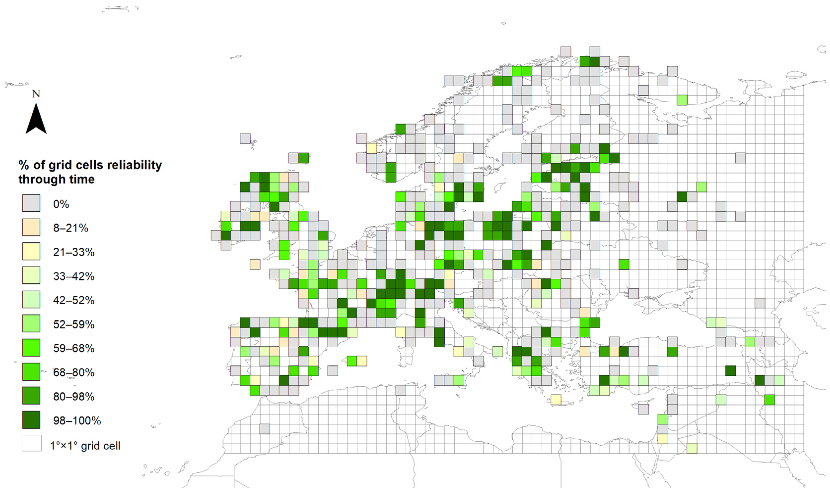
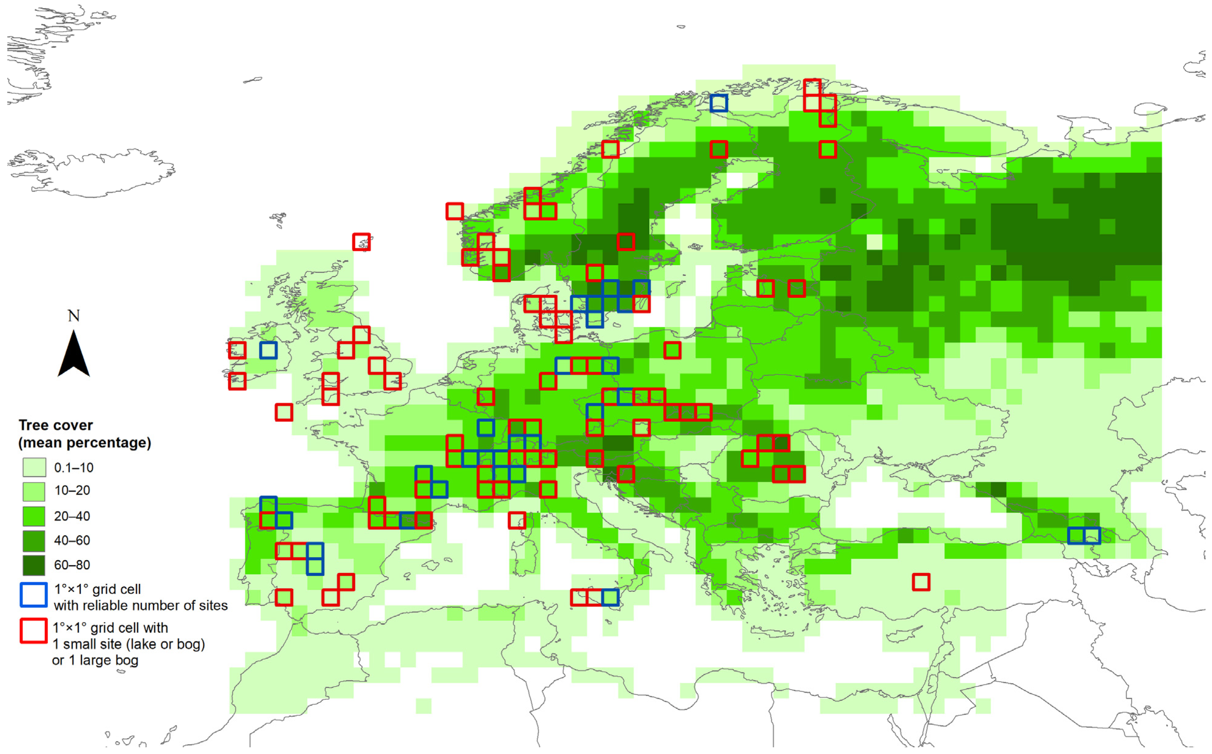
4.4. Importance of the Number of Pollen Records in Europe: Data Reliability

The reliability (quality) of grid-based REVEALS estimates across the Holocene depends on three key elements: the number of pollen records used and their distribution in each grid cell; the type and size of pollen records; and the variation of these factors across time windows [31,33]. The REVEALS model was developed to reconstruct regional vegetation abundance using pollen data from large lakes (>100–500 ha) [27]. Studies using pollen records from the Czech Republic [28], Britain and Ireland [29], and southern Sweden [30] have shown that REVEALS estimates based on pollen records from 2 to 3 small sites (<50 ha) are similar to REVEALS estimates based on pollen records from large lakes. The minimum number of small sites required to obtain reliable outcomes is difficult to define [33]. In this study, we used the “protocol of reliability” proposed earlier [31], considering “reliable” the grid cells with one large lake or at least three small sites. Those grid cells with less than three small sites (lake or bog) or a large bog that violates assumptions of the model (i.e., no pollen-bearing plants grow on the sedimentary basin) were considered “unreliable” (Figure 1). The availability of pollen records from large sites in Europe remains limited, which means that the multiple small sites approach [27] had to be implemented to obtain a larger spatial density of REVEALS estimates across Europe.

Through time, the reliability of an individual grid cell may change, as not all pollen sequences cover the whole Holocene. In this dataset, 186 out of 539 grids are sufficiently reliable (Figure 1) because at least 50% of the time windows are based on large lakes or more than 3 small sites. A total of 62 grid cells are partly reliable as fewer than 50% of the time windows are based on reliable sites or groups of sites. A total of 291 grids are unreliable. Caution should be applied when using REVEALS estimates from unreliable grid cells. These values may still represent regional vegetation if the vegetation in the grid cell was homogeneous in the past, but if the vegetation was heterogenous Gb-RVest from pollen sites that represent local vegetation cover are unlikely to wholly reflect regional vegetation.

The precision of Gb-RVest is indicated by their SEs. Increasing the size of the pollen count for a time window results in RVest with a smaller SE [27,28,31,33]. The 500-year-long time windows (except for the three most recent ones) help to maximize the size of the pollen count for each time window. Caution should be applied when using the Gb-RVest when SEs are equal to or greater than RVest [31].

The results presented here are based on 1607 pollen sequences, which is 40% more than [31], and has greatly improved the availability of reliable Gb-RVest, particularly in southern Europe. Future work should focus on further enhancing this research effort by using more pollen sequences to improve both reliability of values (more sites in each grid cell) and focusing on regions with unreliable grid cells (Figure 1) or where open-source or well-dated sequences are currently lacking. These regions include the Balkan peninsula, Northern Scandinavia, and Eastern and Southern Europe.

5. Conclusions

This paper describes how a different selection of input parameters (three RPP-means datasets, RPPs.sts) affects grid-based REVEALS estimates (Gb-RVest) across the Holocene at a pan-European scale. Using major axis regression, we have shown that the choice of RPP values can result in significant differences in Gb-RVest. RPPs.sts were validated for the first time on a European scale. We had shown that REVEALS performed better when RPPs.st1 was used. This RPP set excluded entomophilous taxa but included those with mixed dispersal mechanisms. Thus, the addition of a larger number of entomophilous taxa does not significantly improve the overall result, and it is more important to obtain reliable RPP values for taxa than broaden the number used. The validation process confirmed earlier studies that have demonstrated that the REVEALS model improves the accuracy of vegetation reconstruction (RVest) significantly over the pollen proportions (raw pollen data) alone.

This study points out the complexity of the variables acting on Gb-RVest. Mainly RPPs values, intrinsic plant characteristics (e.g., entomophily/anemophily, flowers, and pollen morphology), and the place where pollen grains were sampled (lakes or peat bogs) can influence quantified vegetation reconstructions. The increasing number of pollen records used in this study across Europe and during the Holocene has increased the quality and accuracy of vegetation estimates both at the spatial and temporal levels.

This emphasizes the importance of all inputs used in the model and intends to foster the inclusion of numerous factors that act on the pollen grains’ production, dispersion, and deposition when interpreting the estimated results. Thus, it encourages new studies on the improvement of RPPs and pollen records in Europe in order to make the reconstructions increasingly accurate.

The great improvement of the accuracy and spatial coverage of REVEALS-based reconstruction enables better and more detailed usages of these results. Within the Terranova Project, examples of uses are the exploration of spatial-temporal changes in past land cover and biodiversity over long time periods at a European scale, the evaluation of model-simulated vegetation cover from dynamic vegetation model (CARAIB [85]), and Agent-Based Models (ABM [86]), respectively.

References

1. Díaz, S.M.; Settele, J.; Brondízio, E.; Ngo, H.; Guèze, M.; Agard, J.; Arneth, A.; Balvanera, P.; Brauman, K.; Butchart, S.; et al. The Global Assessment Report on Biodiversity and Ecosystem Services: Summary for Policy Makers; IPBES Secretariat: Bonn, Germany, 2019; 1148p. [Google Scholar] [CrossRef]
2. Pörtner, H.O.; Scholes, R.J.; Agard, J.; Archer, E.; Arneth, A.; Bai, X.; Barnes, D.; Burrows, M.; Chan, L.; Cheung, W.L.; et al. Scientific Outcome of the IPBES-IPCC Co-Sponsored Workshop on Biodiversity and Climate Change; Secretariat of the Intergovernmental Science-Policy Platform for Biodiversity and Ecosystem Services; IPBES Secretariat: Bonn, Germany, 2021. [Google Scholar] [CrossRef]
3. Marquer, L.; Gaillard, M.J.; Sugita, S.; Poska, A.; Trondman, A.K.; Mazier, F.; Nielsen, A.B.; Fyfe, R.M.; Jönsson, A.M.; Smith, B.; et al. Quantifying the Effects of Land Use and Climate on Holocene Vegetation in Europe. Quat. Sci. Rev. 2017, 171, 20–37. [Google Scholar] [CrossRef]
4. Poska, A.; Väli, V.; Vassiljev, J.; Alliksaar, T.; Saarse, L. Timing and Drivers of Local to Regional Scale Land-Cover Changes in the Hemiboreal Forest Zone during the Holocene: A Pollen-Based Study from South Estonia. Quat. Sci. Rev. 2022, 277, 107351. [Google Scholar] [CrossRef]
5. Tinner, W.; Hofstetter, S.; Zeugin, F.; Conedera, M.; Wohlgemuth, T.; Zimmermann, L.; Zweifel, R. Long-Distance Transport of Macroscopic Charcoal by an Intensive Crown Fire in the Swiss Alps—Implications for Fire History Reconstruction. Holocene 2006, 16, 287–292. [Google Scholar] [CrossRef]
6. Kalis, A.J.; Merkt, J.; Wunderlich, J. Environmental Changes during the Holocene Climatic Optimum in Central Europe—Human Impact and Natural Causes. Quat. Sci. Rev. 2003, 22, 33–79. [Google Scholar] [CrossRef]
7. Roberts, N.; Fyfe, R.M.; Woodbridge, J.; Gaillard, M.-J.; Davis, B.A.S.; Kaplan, J.O.; Marquer, L.; Mazier, F.; Nielsen, A.B.; Sugita, S.; et al. Europe’s Lost Forests: A Pollen-Based Synthesis for the Last 11,000 Years. Sci. Rep. 2018, 8, 716. [Google Scholar] [CrossRef]
8. Ellis, E.C.; Gauthier, N.; Goldewijk, K.K.; Bird, R.B.; Boivin, N.; Díaz, S.; Fuller, D.Q.; Gill, J.L.; Kaplan, J.O.; Kingston, N.; et al. People Have Shaped Most of Terrestrial Nature for at Least 12,000 Years. Proc. Natl. Acad. Sci. USA 2021, 118, e2023483118. [Google Scholar] [CrossRef]
9. Mottl, O.; Flantua, S.G.A.; Bhatta, K.P.; Felde, V.A.; Giesecke, T.; Goring, S.; Grimm, E.C.; Haberle, S.; Hooghiemstra, H.; Ivory, S.; et al. Erratum: Global Acceleration in Rates of Vegetation Change over the Past 18,000 Years. Science 2021, 373, 860–864. [Google Scholar] [CrossRef]
10. Williams, N.S.G.; Hahs, A.K.; Vesk, P.A. Urbanisation, Plant Traits and the Composition of Urban Floras. Perspect. Plant Ecol. Evol. Syst. 2015, 17, 78–86. [Google Scholar] [CrossRef]
11. Fyfe, R.M.; Woodbridge, J.; Roberts, C.N. Trajectories of Change in Mediterranean Holocene Vegetation through Classification of Pollen Data. Veg. Hist. Archaeobot. 2018, 27, 351–364. [Google Scholar] [CrossRef]
12. Ellis, E.C.; Goldewijk, K.K.; Siebert, S.; Lightman, D.; Ramankutty, N. Anthropogenic Transformation of the Biomes, 1700 to 2000. Glob. Ecol. Biogeogr. 2010, 19, 589–606. [Google Scholar] [CrossRef]
13. Froyd, C.A.; Willis, K.J. Emerging Issues in Biodiversity & Conservation Management: The Need for a Palaeoecological Perspective. Quat. Sci. Rev. 2008, 27, 1723–1732. [Google Scholar] [CrossRef]
14. Willis, K.J.; Bailey, R.M.; Bhagwat, S.A.; Birks, H.J.B. Biodiversity Baselines, Thresholds and Resilience: Testing Predictions and Assumptions Using Palaeoecological Data. Trends Ecol. Evol. 2010, 25, 583–591. [Google Scholar] [CrossRef] [PubMed]
15. Fredh, D.; Broström, A.; Rundgren, M.; Lagerås, P.; Mazier, F.; Zillén, L. The Impact of Land-Use Change on Floristic Diversity at Regional Scale in Southern Sweden 600 BC-AD 2008. Biogeosciences 2013, 10, 3159–3173. [Google Scholar] [CrossRef]
16. Andersen, T.; Carstensen, J.; Hernández-García, E.; Duarte, C.M. Ecological Thresholds and Regime Shifts: Approaches to Identification. Trends Ecol. Evol. 2009, 24, 49–57. [Google Scholar] [CrossRef]
17. Birks, H.J.B.; Felde, V.A.; Seddon, A.W.R. Biodiversity Trends within the Holocene. Holocene 2016, 26, 994–1001. [Google Scholar] [CrossRef]
18. Woodbridge, J.; Fyfe, R.; Smith, D.; Pelling, R.; de Vareilles, A.; Batchelor, R.; Bevan, A.; Davies, A.L. What Drives Biodiversity Patterns? Using Long-Term Multidisciplinary Data to Discern Centennial-Scale Change. J. Ecol. 2021, 109, 1396–1410. [Google Scholar] [CrossRef]
19. Klein Goldewijk, K.; Beusen, A.; Doelman, J.; Stehfest, E. Anthropogenic Land Use Estimates for the Holocene—HYDE 3.2. Earth Syst. Sci. Data 2017, 9, 927–953. [Google Scholar] [CrossRef]
20. Kaplan, J.O.; Krumhardt, K.M.; Ellis, E.C.; Ruddiman, W.F.; Lemmen, C.; Goldewijk, K.K. Holocene Carbon Emissions as a Result of Anthropogenic Land Cover Change. Holocene 2010, 21, 775–791. [Google Scholar] [CrossRef]
21. Hibbard, K.; Janetos, A.; van Vuuren, D.P.; Pongratz, J.; Rose, S.K.; Betts, R.; Herold, M.; Feddema, J.J. Research Priorities in Land Use and Land-Cover Change for the Earth System and Integrated Assessment Modelling. Int. J. Climatol. 2010, 30, 2118–2128. [Google Scholar] [CrossRef]
22. Gaillard, M.-J.; Sugita, S.; Mazier, F.; Trondman, A.-K.; Broström, A.; Hickler, T.; Kaplan, J.O.; Kjellström, E.; Kokfelt, U.; Kuneš, P.; et al. Holocene Land-Cover Reconstructions for Studies on Land Cover-Climate Feedbacks. Clim. Past 2010, 6, 483–499. [Google Scholar] [CrossRef]
23. Willis, K.J.; Birks, H.J.B. What Is Natural? The Need for a Long-Term Perspective in Biodiversity Conservation. Science 2006, 314, 1261–1265. [Google Scholar] [CrossRef] [PubMed]
24. Birks, H.J.B.; Willis, K.J. Alpines, Trees, and Refugia in Europe. Plant Ecol. Divers. 2008, 1, 147–160. [Google Scholar] [CrossRef]
25. Gaillard, M.-J.; Berglund, B.E.; Birks, H.J.B.; Edwards, K.J.; Bittmann, F. “Think Horizontally, Act Vertically”: The Centenary (1916–2016) of Pollen Analysis and the Legacy of Lennart von Post. Veg. Hist. Archaeobot. 2018, 27, 267–269. [Google Scholar] [CrossRef]
26. Prentice, I.C.; Prentice, I.; Webb, T. Pollen Percentages, Tree Abundances and the Fagerlind Effect. J. Quat. Sci. 1986, 1, 35–43. [Google Scholar] [CrossRef]
27. Sugita, S. Theory of Quantitative Reconstruction of Vegetation I: Pollen from Large Sites REVEALS Regional Vegetation Composition. Holocene 2007, 17, 229–241. [Google Scholar] [CrossRef]
28. Mazier, F.; Gaillard, M.J.; Kuneš, P.; Sugita, S.; Trondman, A.K.; Broström, A. Testing the Effect of Site Selection and Parameter Setting on REVEALS-Model Estimates of Plant Abundance Using the Czech Quaternary Palynological Database. Rev. Palaeobot. Palynol. 2012, 187, 38–49. [Google Scholar] [CrossRef]
29. Fyfe, R.M.; Twiddle, C.; Sugita, S.; Gaillard, M.J.; Barratt, P.; Caseldine, C.J.; Dodson, J.; Edwards, K.J.; Farrell, M.; Froyd, C.; et al. The Holocene Vegetation Cover of Britain and Ireland: Overcoming Problems of Scale and Discerning Patterns of Openness. Quat. Sci. Rev. 2013, 73, 132–148. [Google Scholar] [CrossRef]
30. Trondman, A.K.; Gaillard, M.J.; Sugita, S.; Björkman, L.; Greisman, A.; Hultberg, T.; Lagerås, P.; Lindbladh, M.; Mazier, F. Are pollen records from small sites appropriate for REVEALS model-based quantitative reconstructions of past regional vegetation? An empirical test in southern Sweden. Vegetation history and archaeobotany. Veg. Hist. Archaeobot. 2016, 25, 131–151. [Google Scholar] [CrossRef]
31. Githumbi, E.; Fyfe, R.; Gaillard, M.-J.; Trondman, A.-K.; Mazier, F.; Nielsen, A.-B.; Poska, A.; Sugita, S.; Woodbridge, J.; Azuara, J.; et al. European Pollen-Based REVEALS Land-Cover Reconstructions for the Holocene: Methodology, Mapping and Potentials. Earth Syst. Sci. Data 2022, 14, 1581–1619. [Google Scholar] [CrossRef]
32. Strandberg, G.; Lindström, J.; Poska, A.; Zhang, Q.; Fyfe, R.; Githumbi, E.; Kjellström, E.; Mazier, F.; Nielsen, A.B.; Sugita, S.; et al. Mid-Holocene European Climate Revisited: New High-Resolution Regional Climate Model Simulations Using Pollen-Based Land-Cover. Quat. Sci. Rev. 2022, 281, 107431. [Google Scholar] [CrossRef]
33. Trondman, A.K.; Gaillard, M.J.; Mazier, F.; Sugita, S.; Fyfe, R.; Nielsen, A.B.; Twiddle, C.; Barratt, P.; Birks, H.J.B.; Bjune, A.E.; et al. Pollen-Based Quantitative Reconstructions of Holocene Regional Vegetation Cover (Plant-Functional Types and Land-Cover Types) in Europe Suitable for Climate Modelling. Glob. Chang. Biol. 2015, 21, 676–697. [Google Scholar] [CrossRef]
34. Li, F.; Gaillard, M.-J.; Cao, X.; Herzschuh, U.; Sugita, S.; Ni, J.; Zhao, Y.; An, C.; Huang, X.; Li, Y.; et al. Gridded Pollen-Based Holocene Regional Plant Cover in Temperate and Northern Subtropical China Suitable for Climate Modeling. Earth Syst. Sci. Data 2023, 15, 95–112. Available online: https://essd.copernicus.org/preprints/essd-2022-148/ (accessed on 1 December 2022). [CrossRef]
35. Broström, A.; Nielsen, A.B.; Gaillard, M.-J.; Hjelle, K.; Mazier, F.; Binney, H.; Bunting, J.; Fyfe, R.; Meltsov, V.; Poska, A.; et al. Pollen Productivity Estimates of Key European Plant Taxa for Quantitative Reconstruction of Past Vegetation: A Review. Veg. Hist. Archaeobot. 2008, 17, 461–478. [Google Scholar] [CrossRef]
36. Wieczorek, M.; Herzschuh, U. Compilation of Relative Pollen Productivity (RPP) Estimates and Taxonomically Harmonised RPP Datasets for Single Continents and Northern Hemisphere Extratropics. Earth Syst. Sci. Data 2020, 12, 3515–3528. [Google Scholar] [CrossRef]
37. Golam, S.A. Pollen Morphology and Its Systematic Significance in the Ericaceae. Ph.D. Thesis, Hokkaido University, Sapporo, Japan, 2007. [Google Scholar] [CrossRef]
38. Davis, M.B. On the Theory of Pollen Analysis. Am. J. Sci. 1963, 261, 897–912. [Google Scholar] [CrossRef]
39. Sugita, S.; Parshall, T.; Calcote, R.; Walker, K. Testing the Landscape Reconstruction Algorithm for Spatially Explicit Reconstruction of Vegetation in Northern Michigan and Wisconsin. Quat. Res. 2010, 74, 289–300. [Google Scholar] [CrossRef]
40. Sugita, S. A Model of Pollen Source Area for an Entire Lake Surface. Quat. Res. 1993, 39, 239–244. [Google Scholar] [CrossRef]
41. Sutton, O.G. Micrometeorology; McGraw-Hill: New York, NY, USA, 1953. [Google Scholar]
42. Sugita, S. Pollen Representation of Vegetation in Quaternary Sediments: Theory and Method in Patchy Vegetation. J. Ecol. 1994, 82, 881–897. [Google Scholar] [CrossRef]
43. Prentice, C. Records of Vegetation in Time and Space: The Principles of Pollen Analysis. In Vegetation History; Springer: Dordrecht, The Netherlands, 1988; pp. 17–42. [Google Scholar] [CrossRef]
44. Prentice, I.C. Pollen Representation, Source Area, and Basin Size: Toward a Unified Theory of Pollen Analysis. Quat. Res. 1985, 23, 76–86. [Google Scholar] [CrossRef]
45. Parsons, R.W.; Prentice, I.C. Statistical approaches to R-values and the pollen—Vegetation relationship. Rev. Palaeobot. Palynol. 1981, 32, 127–152. [Google Scholar] [CrossRef]
46. Kuparinen, A.; Markkanen, T.; Riikonen, H.; Vesala, T. Modeling Air-Mediated Dispersal of Spores, Pollen and Seeds in Forested Areas. Ecol. Modell. 2007, 208, 177–188. [Google Scholar] [CrossRef]
47. Theuerkauf, M.; Joosten, H. Younger Dryas Cold Stage Vegetation Patterns of Central Europe-Climate, Soil and Relief Controls. Boreas 2012, 41, 391–407. [Google Scholar] [CrossRef]
48. Theuerkauf, M.; Couwenberg, J.; Kuparinen, A.; Liebscher, V. A Matter of Dispersal: REVEALSinR Introduces State-of-the-Art Dispersal Models to Quantitative Vegetation Reconstruction. Veg. Hist. Archaeobot. 2016, 25, 541–553. [Google Scholar] [CrossRef]
49. Marquer, L.; Mazier, F.; Sugita, S.; Galop, D.; Houet, T.; Faure, E.; Gaillard, M.J.; Haunold, S.; de Munnik, N.; Simonneau, A.; et al. Pollen-Based Reconstruction of Holocene Land-Cover in Mountain Regions: Evaluation of the Landscape Reconstruction Algorithm in the Vicdessos Valley, Northern Pyrenees, France. Quat. Sci. Rev. 2020, 228, 106049. [Google Scholar] [CrossRef]
50. Fyfe, R.M.; de Beaulieu, J.-L.; Binney, H.; Bradshaw, R.H.W.; Brewer, S.; Le Flao, A.; Finsinger, W.; Gaillard, M.-J.; Giesecke, T.; Gil-Romera, G.; et al. The European Pollen Database: Past Efforts and Current Activities. Veg. Hist. Archaeobot. 2009, 18, 417–424. [Google Scholar] [CrossRef]
51. Giesecke, T.; Davis, B.; Brewer, S.; Finsinger, W.; Wolters, S.; Blaauw, M.; De Beaulieu, J.-L.; Binney, H.; Fyfe, R.M.; Gaillard, M.-J.; et al. Towards Mapping the Late Quaternary Vegetation Change of Europe. Veg. Hist. Archaeobot. 2014, 23, 75–86. [Google Scholar] [CrossRef]
52. Kuneš, P.; Abrahám, V.; Kovářík, O.; Kopecký, M.; Břízová, E.; Dudová, L.; Jankovská, V.; Knipping, M.; Kozáková, R.; Nováková, K.; et al. Czech Quaternary Palynological Database-PALYCZ: Review and Basic Statistics of the Data. Preslia Česká Kvartérní Pylová Databáze-PALYCZ: Přehled a Základní Statistika. Preslia 2009, 81, 209–238. [Google Scholar]
53. Lerigoleur, E.; Mazier, F.; Jégou, L.; Perret, M.; Galop, D. PALEOPYR: Un Système d’information Pour Les Données Paléoenvironnementales Nord-Pyrénéennes. Ingéniérie Des Systèmes D’information 2015, 20, 63–87. [Google Scholar] [CrossRef]
54. Marinova, E.; Harrison, S.P.; Bragg, F.; Connor, S.; De Laet, V.; Leroy, S.A.; Mudie, P.; Atanassova, J.; Bozilova, E.; Caner, H.; et al. Pollen-derived biomes in the eastern Mediterranean–Black Sea–Caspian-corridor. J. Biogeogr. 2018, 45, 484–499. [Google Scholar] [CrossRef]
55. Goring, S.; Dawson, A.; Simpson, G.L.; Ram, K.; Graham, R.W.; Grimm, E.C.; Williams, J.W. Neotoma: A Programmatic Interface to the Neotoma Paleoecological Database. Open Quat. 2015, 1, 2. [Google Scholar] [CrossRef]
56. Blaauw, M. Methods and Code for “classical” Age-Modelling of Radiocarbon Sequences. Quat. Geochronol. 2010, 5, 512–518. [Google Scholar] [CrossRef]
57. Hansen, M.C.; Potapov, P.V.; Moore, R.; Hancher, M.; Turubanova, S.A.; Tyukavina, A.; Thau, D.; Stehman, S.V.; Goetz, S.J.; Loveland, T.R.; et al. High-Resolution Global Maps of 21st-Century Forest Cover Change. Science 2013, 342, 850–853. [Google Scholar] [CrossRef] [PubMed]
58. Abraham, V.; Oušková, V.; Kuneš, P. Present-Day Vegetation Helps Quantifying Past Land Cover in Selected Regions of the Czech Republic. PLoS ONE 2014, 9, e100117. [Google Scholar] [CrossRef] [PubMed]
59. Stuart, A.; Ord, J.K. Kendall’s Advanced Theory of Statistics, Distrib. Theory, 1; Scientific Research Publishing: Irvine, CA, USA, 1994; Available online: https://ci.nii.ac.jp/naid/10004597057 (accessed on 2 July 2021).
60. Legendre, P.; Legendre, L. Numerical Ecology, 2nd ed.; Elsevier: Amsterdam, The Netherlands, 1998. [Google Scholar]
61. Harper, W.V. Reduced Major Axis Regression. Wiley StatsRef Stat. Ref. Online 2016, 1–6. [Google Scholar] [CrossRef]
62. Woodbridge, J.; Fyfe, R.M.; Roberts, N. A Comparison of Remotely Sensed and Pollen-Based Approaches to Mapping Europe’s Land Cover. J. Biogeogr. 2014, 41, 2080–2092. [Google Scholar] [CrossRef]
63. Bossard, M. CLC2006 Technical Guidelines; European Environment Agency: Copenhagen, Denmark, 2007. [Google Scholar]
64. Kinnebrew, E.; Ochoa-Brito, J.I.; French, M.; Mills-Novoa, M.; Shoffner, E.; Siegel, K. Biases and Limitations of Global Forest Change and Author-Generated Land Cover Maps in Detecting Deforestation in the Amazon. PLoS ONE 2022, 17, e0268970. [Google Scholar] [CrossRef]
65. Cunningham, D.; Cunningham, P.; Fagan, M.E. Identifying Biases in Global Tree Cover Products: A Case Study in Costa Rica. Forests 2019, 10, 853. [Google Scholar] [CrossRef]
66. Tropek, R.; Sedláček, O.; Beck, J.; Keil, P.; Musilová, Z.; Šímová, I.; Storch, D. Comment on “High-Resolution Global Maps of 21st-Century Forest Cover Change”. Science 2014, 344, 850–853. [Google Scholar] [CrossRef]
67. Banskota, A.; Kayastha, N.; Falkowski, M.J.; Wulder, M.A.; Froese, R.E.; White, J.C. Forest Monitoring Using Landsat Time Series Data: A Review. Can. J. Remote Sens. 2014, 40, 362–384. [Google Scholar] [CrossRef]
68. Matthias, I.; Nielsen, A.B.; Giesecke, T. Evaluating the Effect of Flowering Age and Forest Structure on Pollen Productivity Estimates. Veg. Hist. Archaeobot. 2012, 21, 471–484. [Google Scholar] [CrossRef]
69. Coomes, D.A.; Allen, R.B. Effects of Size, Competition and Altitude on Tree Growth. J. Ecol. 2007, 95, 1084–1097. [Google Scholar] [CrossRef]
70. Katz, D.S.W.; Morris, J.R.; Batterman, S.A. Pollen Production for 13 Urban North American Tree Species: Allometric Equations for Tree Trunk Diameter and Crown Area. Aerobiologia 2020, 36, 401–415. [Google Scholar] [CrossRef] [PubMed]
71. Hellman, S.E.V.; Gaillard, M.; Broström, A.; Sugita, S. Effects of the Sampling Design and Selection of Parameter Values on Pollen-Based Quantitative Reconstructions of Regional Vegetation: A Case Study in Southern Sweden Using the REVEALS Model. Veg. Hist. Archaeobot. 2008, 17, 445–459. [Google Scholar] [CrossRef]
72. Hellman, S.; Gaillard, M.-J.; Broström, A.; Sugita, S. The REVEALS Model, a New Tool to Estimate Past Regional Plant Abundance from Pollen Data in Large Lakes: Validation in Southern Sweden. J. Quat. Sci. 2008, 23, 21–42. [Google Scholar] [CrossRef]
73. Bunting, M.J.; Farrell, M.; Broström, A.; Hjelle, K.L.; Mazier, F.; Middleton, R.; Nielsen, A.B.; Rushton, E.; Shaw, H.; Twiddle, C.L. Palynological Perspectives on Vegetation Survey: A Critical Step for Model-Based Reconstruction of Quaternary Land Cover. Quat. Sci. Rev. 2013, 82, 41–55. [Google Scholar] [CrossRef]
74. Bunting, M.J.; Hjelle, K.L. Effect of Vegetation Data Collection Strategies on Estimates of Relevant Source Area of Pollen (RSAP) and Relative Pollen Productivity Estimates (Relative PPE) for Non-Arboreal Taxa. Veg. Hist. Archaeobot. 2010, 19, 365–374. [Google Scholar] [CrossRef]
75. Von Stedingk, H.; Fyfe, R.M.; Allard, A. Pollen Productivity Estimates from the Forest-Tundra Ecotone in West-Central Sweden: Implications for Vegetation Reconstruction at the Limits of the Boreal Forest. Holocene 2008, 18, 323–332. [Google Scholar] [CrossRef]
76. Celikel, G.; Demirsoy, L.; Demirsoy, H. The Strawberry Tree (Arbutus unedo L.) Selection in Turkey. Sci. Hortic. 2008, 118, 115–119. [Google Scholar] [CrossRef]
77. Mesléard, F.; Lepart, J. Germination and Seedling Dynamics of Arbutus Unedo and Erica Arbórea on Corsica. J. Veg. Sci. 1991, 2, 155–164. [Google Scholar] [CrossRef]
78. Sealy, J.R. Arbutus Unedo. J. Ecol. 1949, 37, 365. [Google Scholar] [CrossRef]
79. Fagúndez, J. Two Wild Hybrids of Erica L. (Ericaceae) from Northwest Spain. Bot. Complut. 2006, 30, 131–135. [Google Scholar]
80. Bannister, P. Erica cinerea L. J. Ecol. 1965, 53, 527–542. [Google Scholar] [CrossRef]
81. Wood, C.E. The Genera of Guttiferae (Clusiaceae) in the Southeastern United States. J. Arnlod Arbor. 1976, 57, 74–90. [Google Scholar]
82. Froborg, H. Pollination and Seed Production in Five Boreal Species of Vaccinium and Andromeda (Ericaceae). Can. J. Bot. 1996, 74, 1363–1368. [Google Scholar] [CrossRef]
83. Bell, J.N.B.; Tallis, J.H. Empetrum nigrum L. Source J. Ecol. 1973, 61, 289–305. [Google Scholar] [CrossRef]
84. Castro-Parada, A.; Muñoz Sobrino, C. Variations in Modern Pollen Distribution in Sediments from Nearby Upland Lakes: Implications for the Interpretation of Paleoecological Data. Rev. Palaeobot. Palynol. 2022, 306, 104765. [Google Scholar] [CrossRef]
85. François, L.; Ghislain, M.; Otto, D.; Micheels, A. Late Miocene Vegetation Reconstruction with the CARAIB Model. Palaeogeogr. Palaeoclim. Palaeoecol. 2006, 238, 302–320. [Google Scholar] [CrossRef]
86. Romanowska, I.; Crabtree, S.A.; Harris, K.; Davies, B. Agent-Based Modeling for Archaeologists: Part 1 of 3. Adv. Archaeol. Pr. 2019, 7, 178–184. [Google Scholar] [CrossRef]
87. Grindean, R.; Nielsen, A.B.; Tanţău, I.; Feurdean, A. Relative Pollen Productivity Estimates in the Forest Steppe Landscape of Southeastern Romania. Rev. Palaeobot. Palynol. 2019, 264, 54–63. [Google Scholar] [CrossRef]
88. Li, F.; Gaillard, M.-J.; Xu, Q.; Bunting, M.J.; Li, Y.; Li, J.; Mu, H.; Lu, J.; Zhang, P.; Zhang, S.; et al. A Review of Relative Pollen Productivity Estimates from Temperate China for Pollen-Based Quantitative Reconstruction of Past Plant Cover. Front. Plant Sci. 2018, 9, 1214. [Google Scholar] [CrossRef]
89. Räsänen, S.; Suutari, H.; Nielsen, A.B. A Step Further towards Quantitative Reconstruction of Past Vegetation in Fennoscandian Boreal Forests: Pollen Productivity Estimates for Six Dominant Taxa. Rev. Palaeobot. Palynol. 2007, 146, 208–220. [Google Scholar] [CrossRef]
90. Prentice, I.C.; Parsons, R.W. Maximum Likelihood Linear Calibration of Pollen Spectra in Terms of Forest Composition. Biometrics 1983, 39, 1051. [Google Scholar] [CrossRef]
91. Bunting, M.J.; Armitage, R.; Binney, H.A.; Waller, M. Estimates of ‘relative pollen productivity’ and ‘relevant source area of pollen’ for major tree taxa in two Norfolk (UK) woodlands. Holocene 2005, 15, 459–465. [Google Scholar] [CrossRef]
92. Abraham, V.; Kozáková, R. Relative Pollen Productivity Estimates in the Modern Agricultural Landscape of Central Bohemia (Czech Republic). Rev. Palaeobot. Palynol. 2012, 179, 1–12. [Google Scholar] [CrossRef]
93. Nielsen, A.B. Modelling Pollen Sedimentation in Danish Lakes at c. AD 1800: An Attempt to Validate the POLLSCAPE Model. J. Biogeogr. 2004, 31, 1693–1709. [Google Scholar] [CrossRef]
94. Poska, A.; Meltsov, V.; Sugita, S.; Vassiljev, J. Relative Pollen Productivity Estimates of Major Anemophilous Taxa and Relevant Source Area of Pollen in a Cultural Landscape of the Hemi-Boreal Forest Zone (Estonia). Rev. Palaeobot. Palynol. 2011, 167, 30–39. [Google Scholar] [CrossRef]
95. Theuerkauf, M.; Kuparinen, A.; Joosten, H. Pollen Productivity Estimates Strongly Depend on Assumed Pollen Dispersal. Holocene 2013, 23, 14–24. [Google Scholar] [CrossRef]
96. Hjelle, K.L. Herb Pollen Representation in Surface Moss Samples from Mown Meadows and Pastures in Western Norway. Veg. Hist. Archaeobot. 1998, 7, 79–96. [Google Scholar] [CrossRef]
97. Baker, A.G.; Zimny, M.; Keczyński, A.; Bhagwat, S.A.; Willis, K.J.; Latałowa, M. Pollen Productivity Estimates from Old-Growth Forest Strongly Differ from Those Obtained in Cultural Landscapes: Evidence from the Białowieża National Park, Poland. Holocene 2016, 26, 80–92. [Google Scholar] [CrossRef]
98. Broström, A.; Sugita, S.; Gaillard, M.J. Pollen Productivity Estimates for the Reconstruction of Past Vegetation Cover in the Cultural Landscape of Southern Sweden. Holocene 2004, 14, 368–381. [Google Scholar] [CrossRef]
99. Sugita, S.; Gaillard, M.J.; Broström, A. Landscape Openness and Pollen Records: A Simulation Approach. Holocene 1999, 9, 409–421. [Google Scholar] [CrossRef]
100. Soepboer, W.; Sugita, S.; Lotter, A.F.; van Leeuwen, J.F.N.; van der Knaap, W.O. Pollen Productivity Estimates for Quantitative Reconstruction of Vegetation Cover on the Swiss Plateau. Holocene 2007, 17, 65–77. [Google Scholar] [CrossRef]
101. Mazier, F.; Broström, A.; Gaillard, M.-J.; Sugita, S.; Vittoz, P.; Buttler, A. Pollen Productivity Estimates and Relevant Source Area of Pollen for Selected Plant Taxa in a Pasture Woodland Landscape of the Jura Mountains (Switzerland). Veg. Hist. Archaeobot. 2008, 17, 479–495. [Google Scholar] [CrossRef]
102. Li, F.; Gaillard, M.-J.; Cao, X.; Herzschuh, U.; Sugita, S.; Tarasov, P.E.; Wagner, M.; Xu, Q.; Ni, J.; Wang, W.; et al. Towards Quantification of Holocene Anthropogenic Land-Cover Change in Temperate China: A Review in the Light of Pollen-Based REVEALS Reconstructions of Regional Plant Cover. Earth-Sci. Rev. 2020, 203, 103119. [Google Scholar] [CrossRef]
103. Durbin, J.; Watson, G.S. Testing for Serial Correlation in Least Squares Regression. I. Volume II; Springer: New York, NY, USA, 1992; pp. 237–259. [Google Scholar] [CrossRef]
104. Legendre, P.; Legendre, L. Numerical Ecology in R; Elsevier: Amsterdam, The Netherlands, 2012. [Google Scholar]
105. Warton, D.I.; Wright, I.J.; Falster, D.S.; Westoby, M. Bivariate line-fitting methods for allometry. Biol. Rev. Camb. Philos. Soc. 2006, 81, 259–291. [Google Scholar] [CrossRef] [PubMed]
106. Warton, D.I.; Duursma, R.A.; Falster, D.S.; Taskinen, S. Smatr 3- an R Package for Estimation and Inference about Allometric Lines. Methods Ecol. Evol. 2012, 3, 257–259. [Google Scholar] [CrossRef]
Figure 1. Study area showing grid coverage with available REVEALS-based reconstruction of land-cover. Grid-cell reliability depends on the number and type of pollen records for the 25 time windows (TWs). Reliable: ≥1 large lake(s), ≥2 small lake(s) and/or small bog(s), mix of ≥1 large lake(s) and ≥1 small lake(s) and/or small bog(s); less reliable: 1 bog (large or small) or 1 small lake. Grey grid cells: less reliable results for all TWs. Colour indicate, for each grid cell, the % of the total number of TWs with reliable REVEALS reconstructions of plant cover. For instance, light yellow grid cells imply that reconstructions are reliable for 8–21% of the TWs, while they are less reliable for 79–92% of the TWs; and dark green grid cells indicate that reconstructions are reliable for 98–100% of the TWs, while they are less reliable for 0–2% of the TWs.
Land 12 00986 g001
Figure 2. Grid cells with sites (bogs and lakes) used for validation and tree cover at 2000 AD according to the global forest change dataset [57] in mean percentage cover of the grid cell (1° × 1°). Blue and red grid cells, see the legend. See Methods for the definition of “reliable number of sites” (i.e., implying reliable REVEALS estimates of plant cover). Red grid cells represent less reliable REVEALS reconstructions. Note that the information on the reliability of results in this Figure is valid for the time window –45 to –55 (1995–2005 CE) only.
Land 12 00986 g002
Figure 3. Panels (ac): Major axis (MA) regression between grid-based REVEALS estimates (Gb-RVest) using either RPPs.st1 or RPPs.st2, (a) evergreen trees (Gb-RVest-ET), (b) open land (Gb-RVest-OL), and (c) summer green trees (Gb-RVest-ST). Panels (df): MA regression between grid-based REVEALS estimates using either RPPs.st1 or RPPs.st3, (d) evergreen trees, (e) open land, and (f) summer green trees. The black line is the 1 to 1 relationship, and the red line is the best-fitted relationship.
Land 12 00986 g003
Figure 4. Geolocalisation of the diff.A (see Section 3.2) between grid-based REVEALS estimates (Gb-RVest) for Land-cover types using RPPs.st1 and RPPs.st3, shown as negative values of diff.A for evergreen trees (ET) in panel (a) and positive values of diff.A for open land (OL) in panel (b). Panel (c) shows the maximum values of Ericaceae using RPPs.st3. Panels (df) illustrate the maximum values of Calluna vulgaris, Cyperaceae, and Poaceae using RPPs.st1. Scale range is valid for negative and positive values (panels a,b) from dark blue (−80) to dark red (+80) and for maximum values (panels cf) from light pink (0) to dark red (+80).
Land 12 00986 g004
Figure 5. Geolocalisation of the diff.B (see Section 3.2) between grid-based REVEALS estimates (Gb-RVest) for Land-cover types for RPPs.st1 and grid-based REVEALS estimates for Land-cover types using RPPs.st2, in terms of negative values of evergreen trees (ET) panel (a) and positive values of the open land (OL) panel (b). Panel (c) shows the maximum values of Empetrum using RPPs.st2. Panel (d) illustrates the maximum values of Calluna vulgaris using RPPs.st1. For scale range (see caption of Figure 4).
Land 12 00986 g005
Figure 6. From left to right major axis regression between global forest change trees and REVEALS estimates for tree cover RPPs.st1 (lakes and bogs), global forest change trees and REVEALS estimates for tree cover RPPs.st2 (lakes and bogs), global forest change trees and REVEALS estimates for tree cover RPPs.st3 (lakes and bogs) (panels: ac) and corresponding residuals (panels: fh), major axis regression between global forest change trees and raw pollen data (31 taxa), global forest change trees and raw pollen data (46 taxa) (panels: d,e) and corresponding residuals values graphs below (panels: i,j). Black dots correspond to the grid-cell values used, the dark line is the 1 to 1 relationship, and the red line is the best-fitted relationship.
Land 12 00986 g006
Figure 7. From left to right major axis regression between global forest change trees and REVEALS estimates for tree cover RPPs.st1 (lakes), global forest change trees and REVEALS estimates for tree cover RPPs.st2 (lakes), global forest change trees and REVEALS estimates for tree cover RPPs.st3 (lakes) (panels: ac) and corresponding residuals (panels: fh), major axis regression between global forest change trees and raw pollen data (31 taxa), global forest change trees and raw pollen data (46 taxa) (panels: d,e) and corresponding residuals values graphs below (panels: i,j). Black dots correspond to the grid cells values used, the dark line is the 1 to 1 relationship, and the red line is the best-fitted relationship.
Land 12 00986 g007