Article

Responses of Vegetation Phenology to Urbanisation and Natural Factors along an Urban-Rural Gradient: A Case Study of an Urban Agglomeration on the Northern Slope of the Tianshan Mountains

1
Department of Geography and Tourism, Xinjiang Normal University, Urumqi 830054, China
2
Xinjiang Key Laboratory of Lake Environment and Resources in Arid Zone, Urumqi 830054, China
*
Author to whom correspondence should be addressed.
These authors contributed equally to this work.
Land 2023, 12(5), 1108; https://doi.org/10.3390/land12051108
Submission received: 6 April 2023 / Revised: 14 May 2023 / Accepted: 18 May 2023 / Published: 22 May 2023

Abstract

:
Understanding the responses of vegetation phenology to natural and human disturbances is essential for better understanding ecosystems. In this study, Moderate Resolution Imaging Spectroradiometer data and products were used together with other relevant data to analyse vegetation phenological responses to urbanisation and natural factors in the major urban agglomerations of the Urumqi-Changji, Shihezi-Manasi, and Wusu-Kuidun-Dushanzi regions on the Urban Agglomeration on the Northern Slope of the Tianshan Mountains (UANSTM). Vegetation phenology distributed along an urban-rural gradient showed distinct variability, with start of growing season (SOS), end of growing season (EOS), and growing season length (GSL) occurring earlier, later, and longer, respectively, in urban areas than those in suburban and rural areas. In the Urumqi-Changji region, the earliest SOS, the later EOS, and the longest GSL occurred. Surface urban heat island intensity (SUHII) was most pronounced in the Urumqi-Changji region, with a heat island intensity of 1.77–3.34 °C. Vegetation phenology was influenced by both urbanisation and natural factors, whose contributions were 44.2% to EOS and 61.8% to SOS, respectively. The results of this study emphasise the importance of quantifying the vegetation phenological responses to human disturbances, including climate change, along the urban-rural gradient on the UANSTM.

1. Introduction

Vegetation plays an important role in the exchange of energy and materials in terrestrial ecosystems [1]. Periodically rhythmic changes that plants exhibit in response to environmental changes are referred to as vegetation phenology. Phenology reflects the growth and development cycle and productivity of vegetation [2]. An increase in the air temperature can promote the activity of vegetation enzymes, thereby accelerating vegetation phenology. Temperature is an important factor in vegetation phenology [2,3]. The change in local temperature due to the surface urban heat island (SUHI) effect influences not only the local ecosystem but also its vegetation phenology [1,2].
Urbanisation and human activities have fundamentally changed the landscape and ecology of the land. Rapid urban growth and sprawl have led to the widespread transformation of vegetation, which in turn causes local changes in a variety of biotic conditions, including impermeable aquifers, atmospheric and climatic conditions, and the SUHII [4]. With intensified SUHII and its associated environmental challenges, SUHI-induced high temperatures have become a dominant driver of vegetation phenology in and around cities [5]. However, the interaction between the SUHII and climate change complicates the response mechanisms of urban plant phenology. Compared with those in suburban vegetation phenology, early spring phenology, delayed fall and winter phenology, and a long growing season in urban areas are caused by a surge in the SUHII [6,7]. Germino et al. [8] showed that plant phenology is closely related to temperature, in particular at the start and end of the growing season (EOS), indicating that temperature is a primary driver of vegetation phenology. In recent years, the impact of urbanisation on climate has received considerable scientific attention [4,9,10]. Luo et al. [11] found that the early spring phenology of vegetation was closely associated with urban warming in eastern North America. Ding et al. [12] reported that the urbanisation of the Yangtze River Delta in China has led to an advanced start and delayed end of the vegetation growth season in urban areas, thus lengthening the growing season. Jeong et al. [13] found that increased population density led to an earlier start of the vegetation growth season and a later end of the growing season in Seoul, Korea. The natural environment, urban structure, and scale of interest in this study substantially differ from those of the Yangtze River Delta in China, Seoul in Korea, and the eastern part of North America. In the present study, the study area is surrounded by large areas of bare land, deserts, and sparse vegetation, and urban agglomerations are relatively small and scattered. This study area provides a leverage point to explore not only the extent to which the superposition of natural elements and the SUHII affect vegetation phenology along an urban-rural gradient but also the effects of differences between daytime and night-time urban surface temperatures on vegetation phenology.
As a key integrated economic zone in the economic planning of western China, the urban agglomeration on the northern slope of the Tianshan Mountains (UANSTM) has a unique geographical location and natural resource conditions. However, only a few studies have been conducted on the UANSTM in the arid region of Xinjiang, China, and the ecological and environmental challenges in this region remain to be addressed. Therefore, this study considered this region the study area and used Moderate Resolution Imaging Spectroradiometer (MODIS) MOD11A2, MCD12Q2, and MOD13Q1 Enhanced Vegetation Index (EVI) products during 2001–2020 to extract vegetation phenology and surface urban heat island intensity (SUHII) and quantify the spatiotemporal changes in vegetation phenology and SUHII in the three urban clusters of the Urumqi-Changji, Shihezi-Manasi, and Wusu-Kuidun-Dushanzi districts. Thus, the objective of this study was to quantify the effects of urban structure, scale, and population on vegetation phenology along an urban-rural gradient based on the detection of spatiotemporal changes in vegetation phenology and SUHII in the three major urban clusters.

2. Study Area and Data
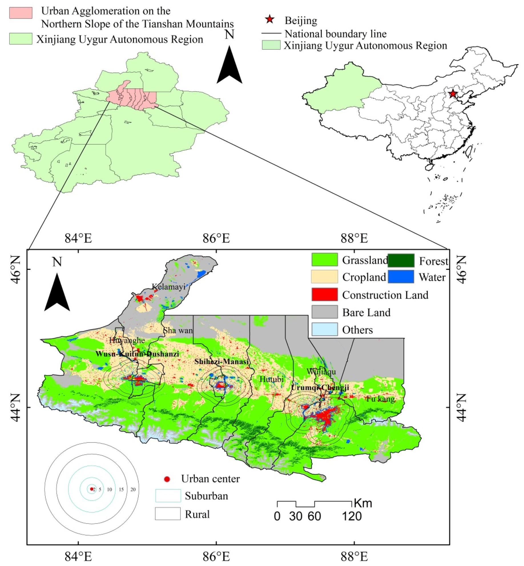
2.1. Study Area

The UANSTM is located in the central part of the Tianshan Mountains and the southern part of the Junggar Basin (Figure 1). The total study area was 95,400 km2, accounting for 5.8% of the total area of Xinjiang, and the population was 8.92 million, accounting for 38.10% of the total population of Xinjiang. With the implementation of the “Western Development Strategy” of China, the study area has become the most economically developed region of Xinjiang and an important hub of the “Silk Road Economic Belt”, as well as one of the 19 key areas of Chinese comprehensive territorial development. The topography of the study area is complex, and the climate type belongs to an arid continental climate with an average annual temperature of 7.5 ± 0.1 °C, an average annual precipitation of 215 mm, and a potential evaporation of 1210 mm, with evaporation being higher than precipitation. The mainland-use and land-cover types are grassland, cropland, forest land, water, construction land, and bare land (28.4% of the area); the main vegetation types are trees, shrubs, herbs, mixed forests, and deciduous coniferous forests; and the ecological environment of the study area is extremely fragile [14]. With increased human disturbances and the construction of UANSTM, the region has experienced rapid urban expansion and increasingly significant urbanisation, making it an ideal test area for elucidating the mechanisms of vegetation phenological changes due to urbanisation in an arid zone.

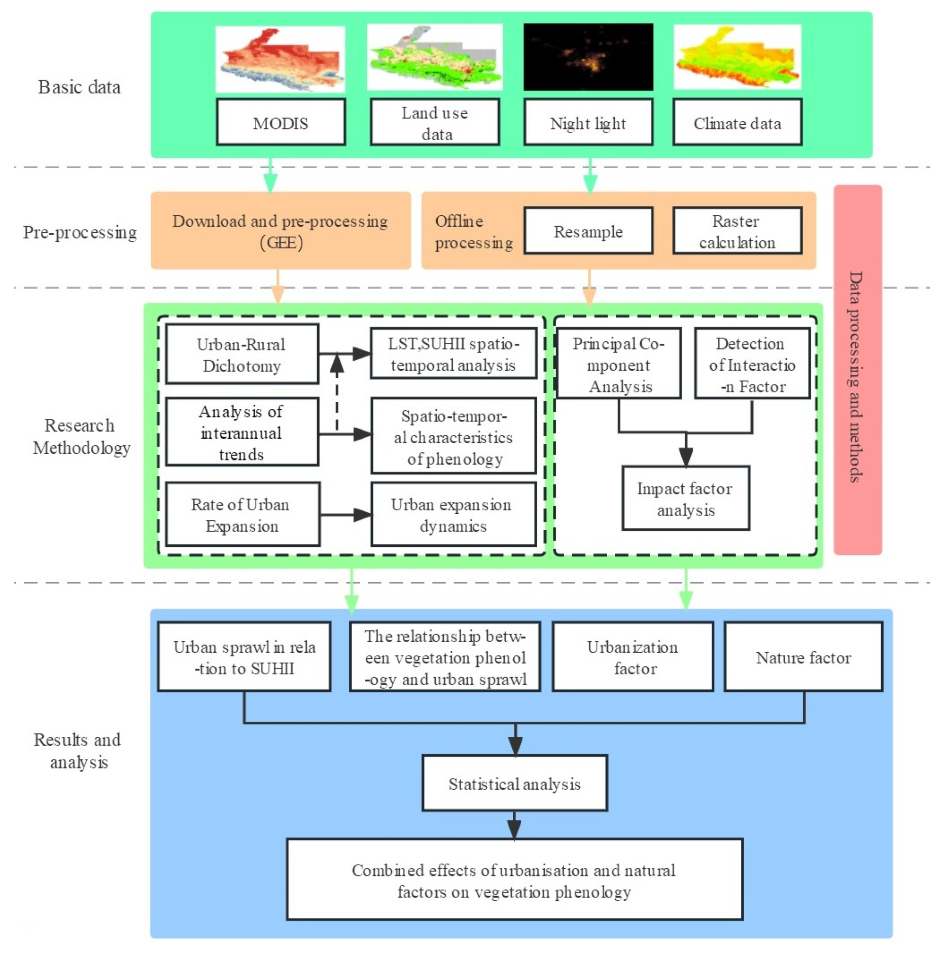
2.2. Data and Processing

As a weather product of the MODIS data, MCD12Q2 includes weather information such as the start of the growing season (SOS), the EOS, and the growing season length (GSL) [15]. Validation results showed that MCD12Q2 has high accuracy in the Xinjiang region, with a coefficient of correlation (r) value of 0.75 (p < 0.05) between the greening period and ground observation. The weather products satisfactorily reflect the spatial distribution of vegetation conditions in the Xinjiang region and meet the research accuracy requirements [16]. The MCD12Q2 and MOD13Q1 data for the study area during 2001–2019 were pre-processed and downloaded from the Google Earth Engine. Since the MCD12Q2 product was not updated to 2020, the EVI and NDVI values of the MOD13Q1 data are important indicators for detecting plant phenology, and EVI can reflect vegetation phenology more accurately than NDVI [16]. The present study estimated the vegetation phenology of the study area in 2020 based on the EVI data of MOD13Q1 by comparing and validating the MOD13Q1 product of the same year with the inverse phenology results, and then corrected the estimated phenology information of the study area in 2020. The MOD11A2 data are ideal for studying SUHII on a large regional scale with high accuracy, with an absolute error of ±1 K [17,18]. The global “National Polar-orbiting Partnership (NPP) Visible Infrared Imager Radiometer Suite (VIIRS)-like” night-time light data with cross-sensor calibration was used for night-time light data [19]. Land-use data were used to define the three major urban agglomerations in the study area. Monthly average temperature and precipitation data for China were extracted and processed in batches using Python. A digital elevation model (DEM) was used to classify vegetation parameters and analyse the variational characteristics of elevation. All data were resampled to maintain a consistent spatial resolution. The specific data sources and parameters are listed in Table 1.

3. Methods

In this study, the UANSTM was used as the study area. Based on the MOD11A2 surface temperature product and the MCD12Q2 vegetation phenology product, the urban-rural dichotomy method was used to calculate the SUHII values and phenological periods of urban agglomerations and analyse their temporal trends and spatial characteristics. Finally, the effects of urbanisation and natural factors on vegetation phenology were analysed. This article utilises corresponding monthly and annual scale datasets with the same time resolution as surface temperature and vegetation phenology data in the study area, as well as other remote sensing data for resampling analysis, to obtain a unified resolution dataset. The technical route is illustrated in Figure 2.

3.1. Urban-Rural Dichotomy

3.1.1. Determining Urban-Rural Boundaries

To calculate the SUHII value of the study area by using the urban-rural dichotomy method, the premise was to first determine the city and township boundaries and then extract the surface temperatures of the city and township. Due to the complex topography and scattered urban areas in the study area, unifying the vector data of the administrative city-county streets was impossible; therefore, accurately determining the city and township boundaries was difficult. In this study, township boundaries were determined using night-time lighting, land-use types, and elevation extracted by Yong Hong et al. [20]. Urbanisation within 10–20 km of urban centres has been shown to exert a significant effect on vegetation phenological differences [21,22]. Therefore, five concentric buffer rings (urban centre, suburban area, 2–15 km, and rural area, 15–20 km) were established for the three urban clusters using the urban built-up area as the centre, extracted from the night-time lighting and land-use data. The buffer rings were used as the urban-rural gradient boundaries. The land-use and night lighting data were used to distinguish between the main urban area and non-main urban areas (arable land, shrub land, grassland, and forest land) and establish a 20 km buffer zone outward from the main urban area as a suburban area [20]. The DEM data were then used to remove bare land and other land types with elevations higher than 1500 m to avoid interference from the cold island effect on SUHII [23].

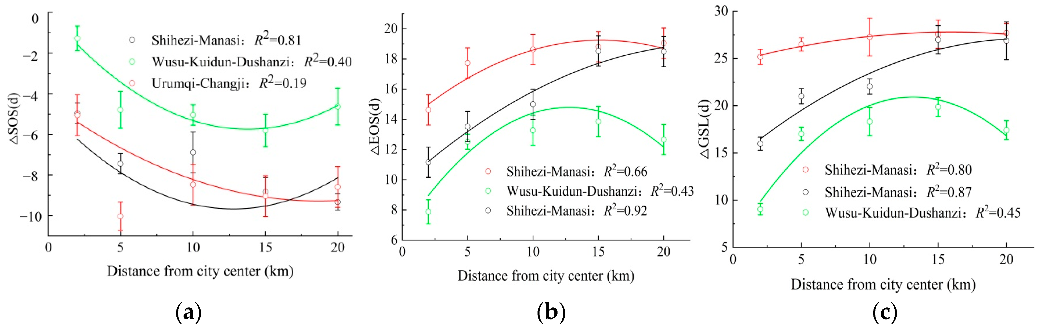
3.1.2. Differences in Vegetation Phenology between Urban and Rural Gradients and SUHII

Based on a comprehensive consideration of the 2001, 2010, and 2020 land-use data in the study area, a buffer zone analysis was conducted for the Urumqi-Changji, Shihezi-Manasi, and Wusu-Kuidun-Dushanzi regions. The values of ΔSOS (d), ΔEOS (d), and ΔGSL (d) were calculated using the differences in SOS, EOS, and GSL between urban centres, suburbs, and rural areas, respectively, as follows:
Δ S O S i = S O S u r b a n   c e n t e r S O S i
Δ E O S i = E O S u r b a n   c e n t e r E O S i
Δ G S L i = G S L u r b a n   c e n t e r G S L i
where ΔSOSi, ΔEOSi, and ΔGSLi are the differences of the average SOS, EOS, and GSL of each buffer zone in the urban centre, suburban area, and rural area, respectively; SOSurban centre, EOSurban centre, and GSLurban centre are the averages of the urban centre SOS, EOS, and GSL, respectively; and SOSi, EOSi, and GSLi are the averages of the SOS, EOS, and GSL for suburban and rural areas, respectively. The difference in land surface temperature (LST) between the urban centre, suburban, and rural areas is then used to express SUHII (°C) as follows:
S U H I I i = T u r b a n   c e n t e r T i
where SUHIIi is the SUHII of each buffer zone in the suburban and rural areas; Turban centre is the average LST of the city centre; and Ti is the average LST for each buffer zone in the suburban and rural areas.

3.2. Average Annual Rate of Urban Expansion

The average annual expansion rate is an indicator used to evaluate the spatial expansion of a city, and its magnitude reflects the rate of urban expansion [24]. Thus:
V r = T S b S a 1 × 100 %
where Vr is the expansion velocity (km2·a−1); Sb and Sa are the urban areas (km2) at the beginning and end of the study, respectively; and T is the time interval (yr).

3.3. Statistical Analysis

The Pearson’s correlation coefficient (r) is widely used in statistical analysis to measure the degree of correlation between two variables and has a value between −1 and 1 [25]. The coefficient of determination (R2) indicates the extent to which the dependent variable is explained by the independent variable in the regression relationship, and its value is equal to the square of r. The larger the value, the higher the degree of explanation for the variation in the response variable [26].

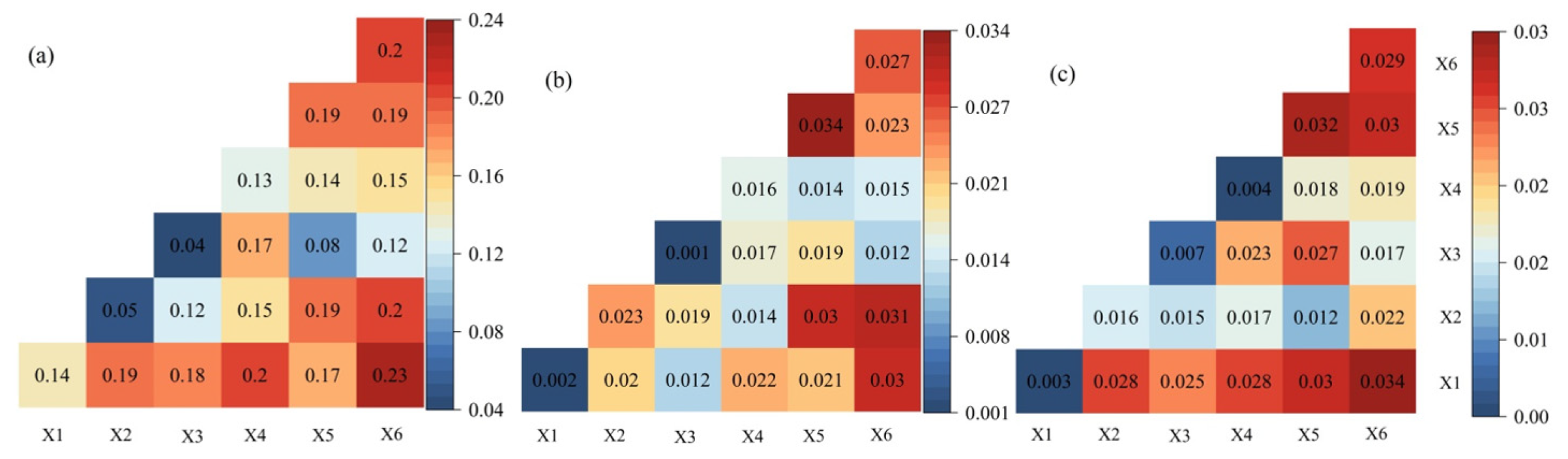
3.4. Detection of Interaction Factors

Geographic detectors can detect the spatial differentiation of geographical phenomena and quantitatively reveal the explanatory power of factors that influence spatial differentiation [27]. The detectors can be classified into factors, interactions, risks, and ecological detection methods. An interaction detector can detect the interactions between different factors and evaluate whether there is an increase or decrease in the effect on vegetation phenology when factors x1 and x2 work together. First, the explanatory powers of x1 and x2 on vegetation phenology were calculated, namely q(x1) and q(x2). Furthermore, q was calculated, i.e., q(x1∩x2) when x1 and x2 interacted, and the sum of q(x1), q(x2), and q(x1 ∩ x2) was compared [28,29].

3.5. Principal Component Analysis and Variance Contribution Rate

Principal component analysis is a statistical method by which a set of potentially correlated variables is transformed into a set of linearly uncorrelated variables via orthogonal transformation; thus, the transformed set of variables is called a principal component [30]. The principal component contribution is the proportion of the variance of the principal component to the total variance of the random variable of interest. It is primarily used to measure the explanatory power of principal components for the variability of the original variables. In the present study, we used the variance contribution ratio to analyse the explanatory power of urbanisation and natural factors for vegetative phenology.

4. Results and Analysis

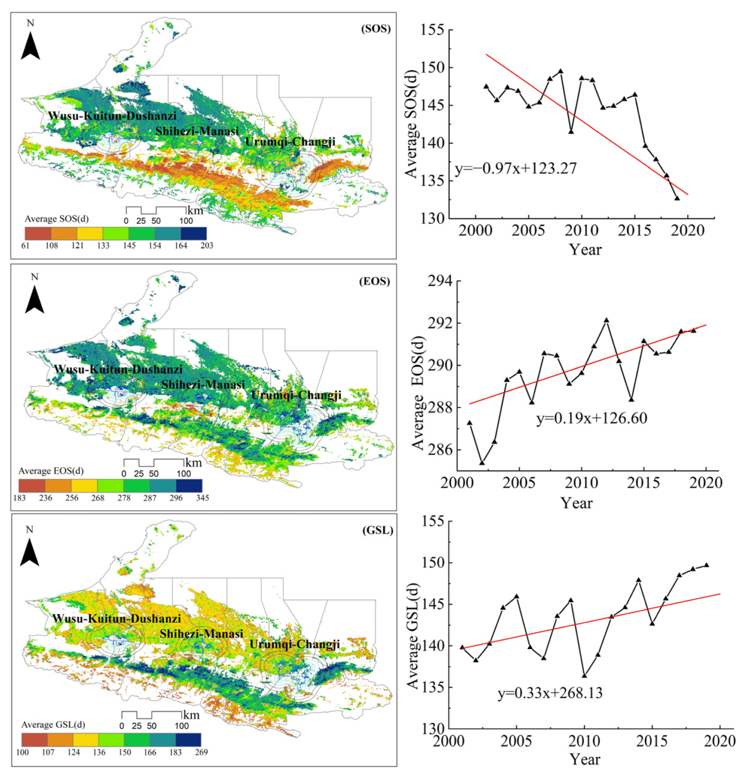
4.1. Spatial and Temporal Evolutionary Characteristics of Vegetation Phenology

During 2001–2020, the SOS value in the study area was in the range of 108–203 d, with a multi-year mean of 142.44 d. The range of EOS and GSL was 236–345 d with a multi-year mean of 282.32 d and 107–269 d with a multi-year mean of 140.03 d, respectively (Figure 3). The smallest mean SOS value was 125.21 d in the Urumqi-Changji region, followed by the Shihezi-Manasi (139.21 d) and Wusu-Kuidun-Dushanzi (145.25 d) regions. The mean EOS value in the Urumqi-Changji region was the highest (302 d), followed by the Wusu-Kuidun-Dushanzi (300.39 d) and Shihezi-Manasi (299.81 d) regions. The mean GSL value in the Urumqi-Changji region was the largest (173.79 d), followed by the Shihezi-Manasi (160.60 d) and Wusu-Kuidun-Dushanzi (155.14 d) regions. The overall variation in the vegetation phenological period in the urban clusters during 2001–2020 was significant, and variability was observed in SOS, EOS, and GSL in the urban clusters at different time periods. The SOS values decreased over time throughout the study area, indicating that the vegetation growth period advanced gradually. The increasing EOS values indicated that the EOS values were delayed gradually, thus extending the GSL value in the study area.
As shown in Figure 4, the farther away it was from the city centre, the smaller the multi-year average value of ΔSOS was; in other words, the distance from the city centre showed a negative correlation with ΔSOS. The average ΔSOS value was 8.24 d (R2 = 0.19, p < 0.05) for the Urumqi-Changji region, 7.40 d (R2 = 0.81, p < 0.01) for the Shihezi-Manasi region, and 4.31 d (R2 = 0.40, p < 0.05) for the Wusu-Kuidun-Dushanzi region. The multi-year average ∆EOS value of the study area rose with increasing distance from the urban centre. The mean ΔEOS was 17.77 d (R2 = 0.66, p < 0.01) in the Urumqi-Changji region, 15.34 d (R2 = 0.92, p < 0.01) in the Shihezi-Manasi region, and 12.04 d (R2 = 0.43, p < 0.05) in the Wusu-Kuidun-Dushanzi region. The multi-year average ∆GSL value of the study area also rose with the increasing distance from the urban centre. The mean ΔGSL value was 16.84 d (R2 = 0.80, p < 0.01) in the Urumqi-Changji region, 12.57 d (R2 = 0.45, p < 0.01) in the Shihezi-Manasi region, and 6.33 d (R2 = 0.87, p < 0.01) in the Wusu-Kuidun-Dushanzi region. These findings indicated that the SUHII in the study area significantly influenced the vegetation phenology in the surrounding area.

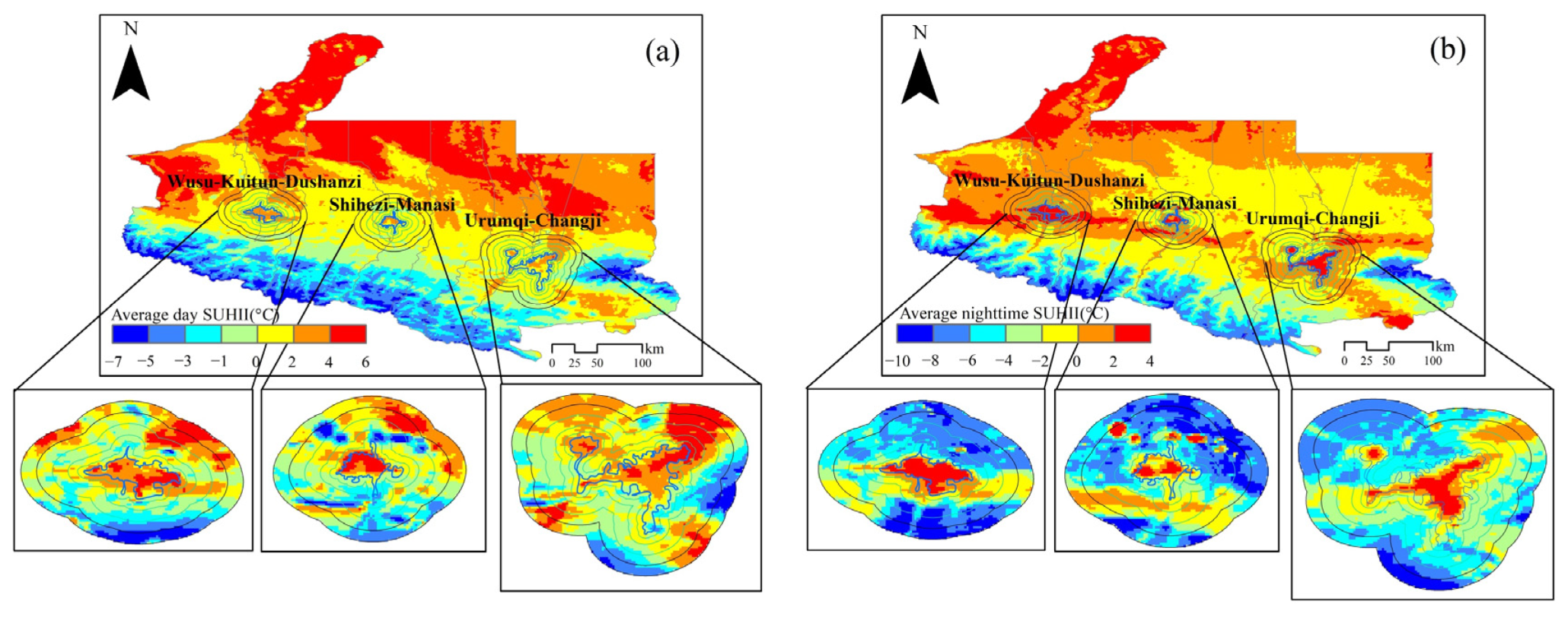
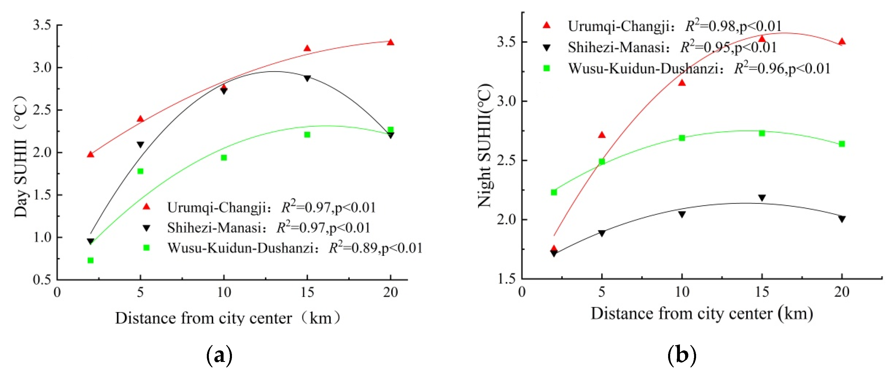
4.2. Spatial and Temporal Distribution Characteristics of Diurnal SUHII

The spatial pattern of SUHII in the urban agglomerations was estimated using the urban-rural dichotomy, and the distance of SUHII from the urban centre was analysed (Figure 5). The average SUHII value of the study area during 2001–2020 ranged from −7 °C to 6 °C during the day and −10 °C to 4 °C at night, with a large difference in the diurnal SUHII value. A high daytime SUHII was concentrated in the northern part of the study area, that is, the desert and sparsely vegetated areas, with cold island effects occurring in the south and southeast. The high SUHII at night was concentrated in the central part of the study area, that is, the inner-city area. The multi-year average SUHII value ranged from 1.97 °C to 3.29 °C and 1.75 °C to 3.52 °C during the day and at night in the Urumqi-Changji region, 0.96 °C to 2.88 °C and 1.72 °C to 2.05 °C in the Shihezi-Manasi region, and 0.73 °C to 2.27 °C and 2.23 °C to 2.69 °C in the Wusu-Kuidun-Dushanzi region, respectively.
As shown in Figure 6, with the increased distance from the urban centre, the multi-year average SUHII value of the study area first rose and then fell; in other words, the distance along the urban-rural gradient showed a significant non-linear relationship with the multi-year average SUHII value. The high SUHII values were mainly located 10–20 km from the urban centre, which was mainly due to the large temperature difference between the urban centre and the suburban and rural areas. The corresponding SUHII peaks of 3.29 °C and 3.52 °C occurred at 15 km from the Urumqi-Changji urban centre during the day and night. During the daytime, 2–6 km from the urban centre, the SUHII values were the highest for Urumqi-Changji, followed by Shihezi-Manasi and Wusu-Kuidun–Dushanzi. At night, 5–20 km from the city centre, the SUHII values were highest in the Urumqi-Changji region, followed by the Wusu-Kuidun-Dushanzi and Shihezi-Manasi regions.

4.3. Response of Vegetation Phenology to Urbanisation

4.3.1. Responses of Vegetation Phenology to Urban Economy and Population Size

A Pearson’s correlation analysis was performed between the urbanisation level and vegetation phenology in the UANSTM. Variability existed in the effects of the three urbanisation levels in the different urban agglomerations on the vegetation phenology in the different cities. The urbanisation level of the urban clusters was correlated negatively with SOS but positively with EOS and GSL (Figure 7). Given the r values, the correlation was weak between the low urbanisation level and vegetation phenology in the urban clusters but strong between the medium-to-high urbanisation levels and vegetation phenology. The average r values were −0.61, −0.59, and −0.77 between the urbanisation level and SOS; 0.77, 0.67, and 0.73 between the urbanisation level and EOS; and 0.72, 0.62, and 0.80 between the urbanisation level and GSL in the Urumqi-Changji, Shihezi-Manasi, and Wusu-Kuidun-Dushanzi districts, respectively. In other words, the Wusu-Kuidun-Dushanzi district showed the strongest correlation with SOS and GSL, followed by the Urumqi-Changji and Shihezi-Manasi districts, whereas the Urumqi-Changji district exhibited the strongest correlation with EOS, followed by the Wusu-Kuidun-Dushanzi and Shihezi-Manasi districts. For the Urumqi-Changji region, the low urbanisation level did not exert a significant impact on SOS and GSL but had a significant impact on EOS. The medium-to-high urbanisation levels showed a greater effect and correlation at the start and end of growing seasons than did the low urbanisation levels.

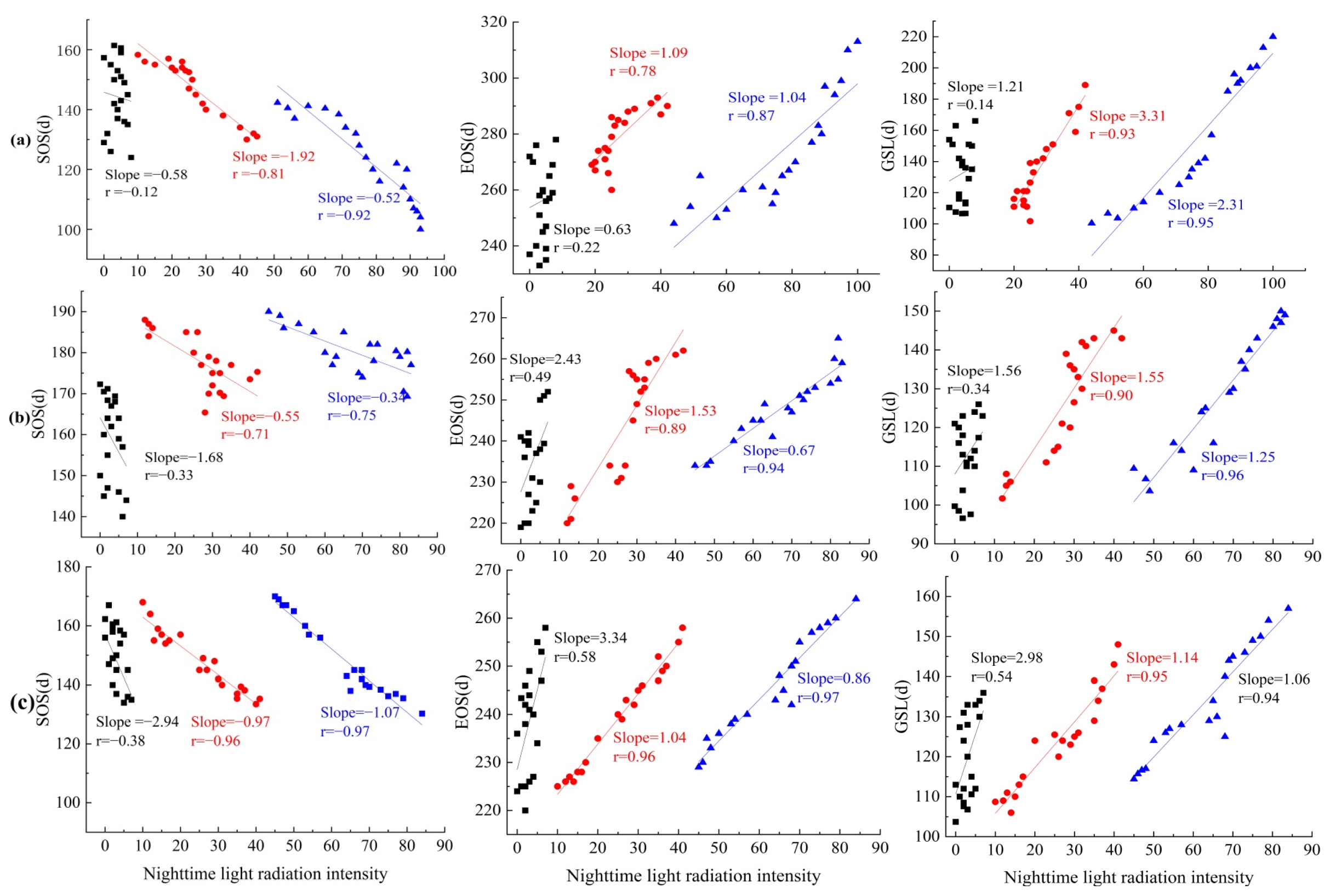
4.3.2. Response of Vegetation Phenology to the Scale of Urban Expansion

Pearson’s r values were obtained for the vegetation phenological period and percentage of built-up land area in the urban, suburban, and rural areas of the Urumqi-Changji, Shihezi-Manasi, and Wusu-Kuidun-Dushanzi districts during 2001–2020 (Table 2). There was a significant correlation (p < 0.01) between the vegetation phenology and the fraction of built-up land area in the urban centre and rural areas of Urumqi-Changji; however, no such significant correlation was observed in the suburban area. The percentage of built-up land in the different areas was strongly correlated negatively with SOS but positively with EOS and GSL. Unlike the vegetation phenology period in the suburban area, the vegetation phenology period in the urban centre of the Shihezi-Manasi district was significantly correlated (p < 0.05) with the percentage of construction land area. In rural areas, EOS was significantly correlated with the percentage of built-up land (p < 0.05). The percentage of built-up land area in the different areas was correlated positively with EOS and GSL but negatively with SOS. The proportion of built-up land area in the Wusu-Kuidun-Dushanzi region was strongly correlated negatively with SOS but positively with EOS and GSL. The percentage of construction land area in the urban and rural areas was significantly correlated with the vegetation phenological period, which was absent in the suburban areas. Therefore, the vegetation phenological period in the Urumqi-Changji and Wusu-Kuidun-Dushanzi districts was significantly influenced by urban expansion and scale. The increased proportion of the construction land area advanced SOS, delayed EOS, and extended GSL in the urban centres.

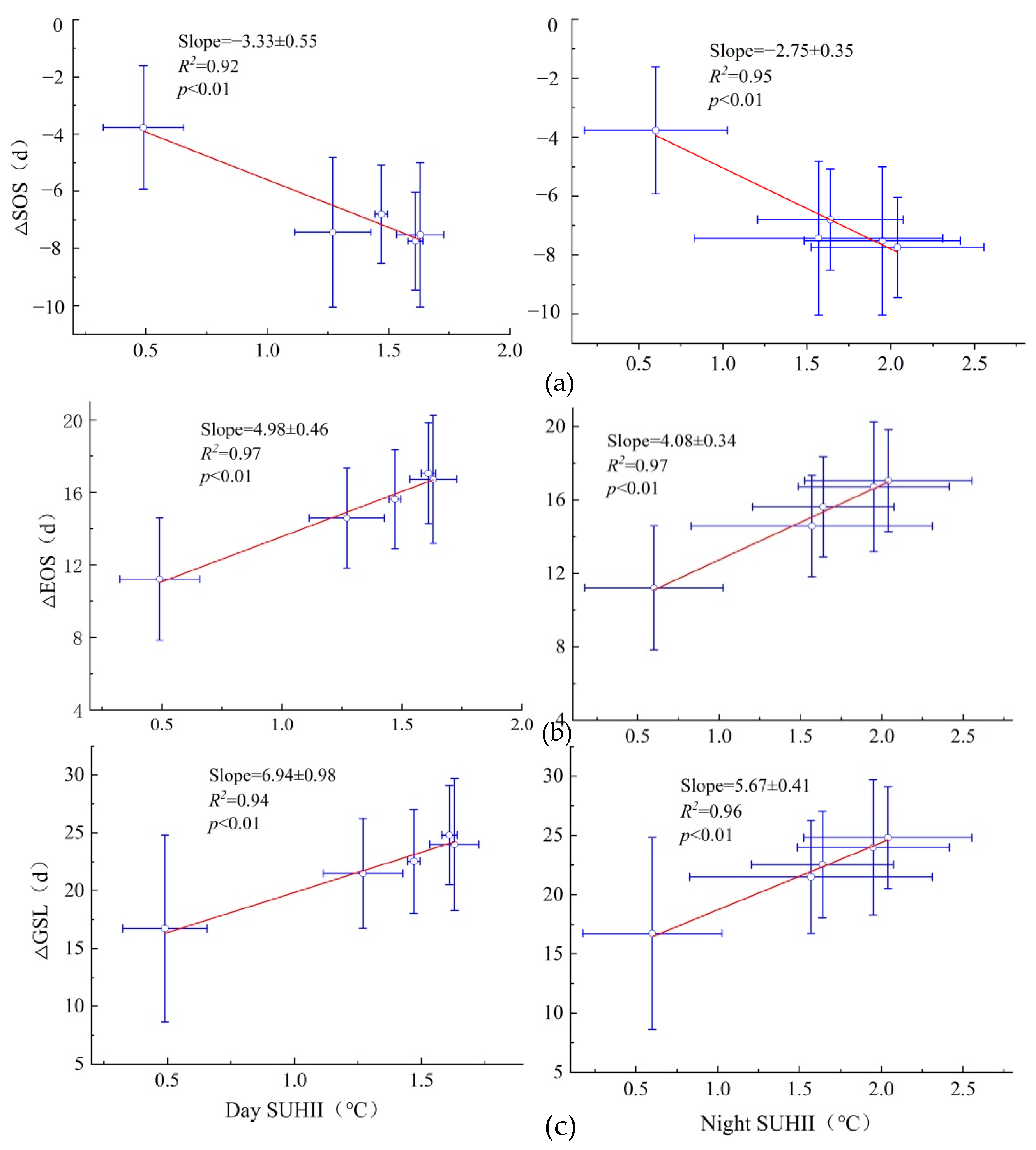
4.3.3. Response of Vegetation Phenology to the SUHI Effect

To establish the relationship of SUHII with the three vegetation phenological variables, the R2 values between SUHII and ΔSOS, ΔEOS, and ΔGSL were separately estimated for the urban clusters. As shown in Table 3, the correlation between the SUHII and vegetation phenology was stronger in the Urumqi-Changji region than in the other two regions, with an average R2 value of 0.94, followed by the Shihezi-Manasi and Wusu-Kuidun-Dushanzi regions, with average R2 values of 0.92 and 0.86, respectively. There was a significant negative correlation between SUHII and ΔSOS in the entire urban agglomeration; that is, the stronger the SUHII value was, the earlier the SOS value was. The SUHII value was highly positively correlated with ΔEOS and ΔGSL; in other words, the stronger the SUHII value was, the later the EOS value was, and the longer the GSL value was. The r values between the SUHII and vegetation phenology were smaller during the day than at night in the Urumqi-Changji and Shihezi-Manasi regions, but higher during the day than at night in the Wusu-Kuidun-Dushanzi region.
As shown in Figure 8, in the study area, SUHII was significantly correlated negatively with ΔSOS (R2 = 0.93, p < 0.01) but highly positively with ΔEOS and ΔGSL (R2 = 0.95, p < 0.01). The stronger the SUHII value was, the earlier the SOS value was, the later the EOS value was, and the longer the GSL value was. When SUHII was raised by 0.1 °C during the day and at night, ΔSOS was advanced by 1.10 d and 1.35 d (mean 1.22 d), ΔEOS was delayed by 1.31 d and 1.08 d (mean 1.19 d), and ΔGSL was prolonged by 1.93 d and 1.59 d (mean 1.76 d), respectively. The SUHII increased the average temperature of the city, particularly at night when warming was greatest. The heat island intensity in the study area was greater at night than during the day, and the R2 values of SUHII with ΔSOS and ΔGSL were higher at night than during the day.

4.4. Responses of Vegetation Phenology to Natural Factors

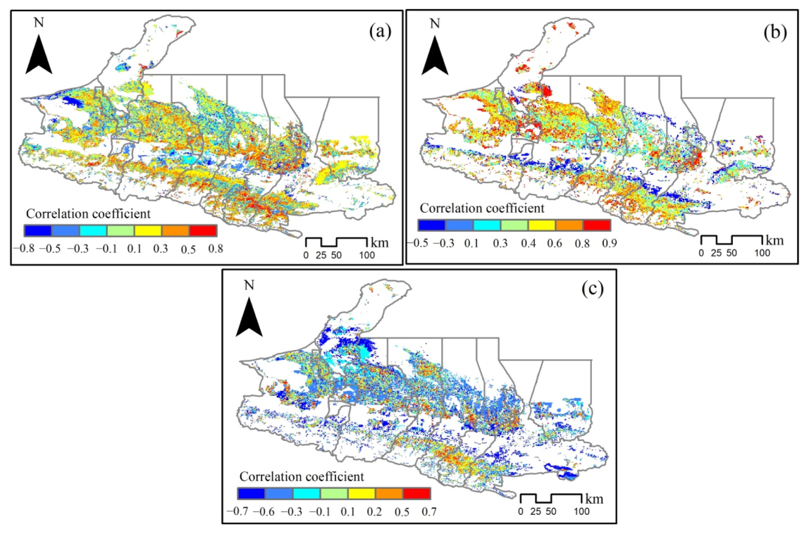
4.4.1. Response of Vegetation Phenology to Precipitation

Based on the spatially skewed r values between the vegetation phenology and precipitation in the entire study area, 48.3% of the negative correlations between SOS and precipitation were found to occur in the northwestern and central areas of the study area; that is, the more precipitation there was in the grassland and cropland areas of the study area, the earlier the SOS value was. With 44.2% of the positive correlations occurring in the southern and southeastern parts of the study area and with 7.3% showing a highly significant positive correlation, the SOS value pointed to a later period with more precipitation in the forested areas. The r values of 0.3–0.8 were mainly concentrated at high elevations (Figure 9a). Approximately 49.1% of the negative correlations between the EOS and precipitation occurred in the northeastern and southern woodland areas of the study area, indicating that more precipitation in the woodlands resulted in an earlier EOS value. Approximately 50.1% of the positive correlations occurring in the northwestern and southern cropland areas of the study area indicated that the higher the precipitation in the study area was, the later the EOS value was, with 9.2% showing a highly significant positive correlation and a uniform spatial distribution (Figure 9b). The areas with r values < 0 between GSL and precipitation were relatively large and showed spatial heterogeneity, and the negative correlation between GSL and precipitation was strong, indicating that the increased precipitation would shorten GSL in most areas (Figure 9c). In conclusion, the response of the vegetation phenology, in particular EOS, to precipitation was highly significant.

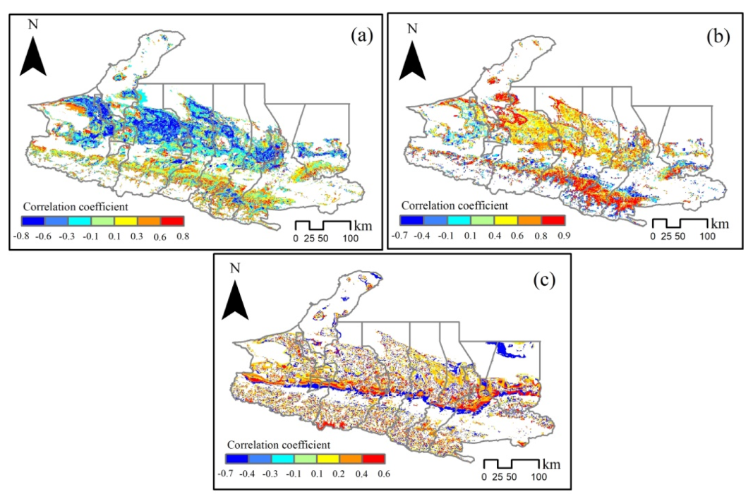
4.4.2. Response of Vegetation Phenology to Temperature

From the spatially skewed r values between the vegetation phenology and air temperature across the study area, we found that 77.7% of the negative correlations between SOS and air temperature occurred in the northern part of the study area, whereas 22.1% of the positive correlations occurred in the southern part of the study area. The r values between temperature and SOS were mainly negative, indicating that the temperature rise advanced SOS. Conversely, a decrease in temperature delayed SOS (Figure 10a). These results were consistent with the characteristics of vegetation growth and development, in which increased temperature raised the accumulation temperature, which then accelerated vegetation growth and development, thus resulting in an earlier SOS value. The r values between EOS and temperature were mainly positive (Figure 10b). The western and southern regions of the study area exhibited a significant positive correlation. In other words, EOS clearly responded to the temperature, and the increased temperature caused a delay in EOS. Conversely, EOS occurred earlier, when the temperature decreased. The correlation between GSL and temperature was insignificant and spatially heterogeneous (Figure 10c). Overall, the response of the vegetation phenology was slightly stronger to the temperature than to the precipitation, and the effects of SOS and EOS were significant.

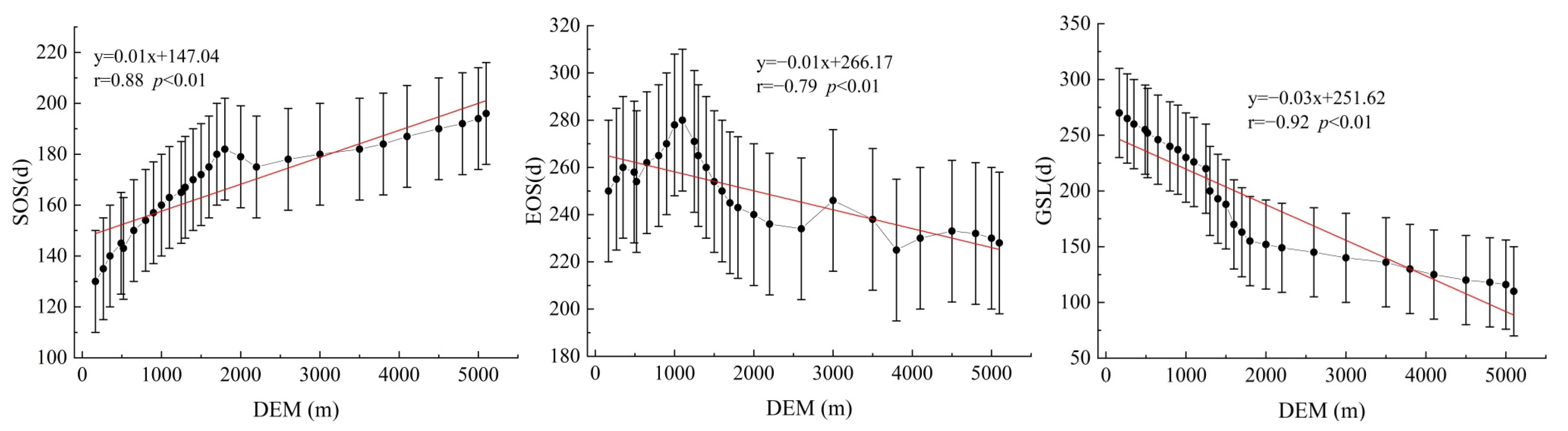
4.4.3. Response of Vegetation Phenology to Elevation

A close relationship was observed between vegetation phenology and altitude in the UANSTM (Figure 11). The correlation between SOS and altitude was more significant (p < 0.01) between 1000 and 2000 m above sea level (asl) than between 2500 and 5000 m asl. The SOS value was significantly delayed with the increasing altitude, advancing 2.5 d for a 100 m altitudinal rise. The correlation between EOS and altitude was significant, with EOS being significantly delayed with the increasing altitude between 200 and 1000 m, more significantly correlated between 1000 and 2500 m (p < 0.01), significantly advanced with the increasing altitude, and less significantly correlated between 2500 and 5000 m. For every 100 m of elevation increase, the EOS value was 2.5 d ahead. The GSL and altitude values showed a significant correlation; GSL shortened with increasing altitude, and the shortening of GSL was most pronounced in the range of 200–1000 m (p < 0.01). The GSL value was shortened by 2.5 d per 100 m of altitudinal rise. Studies have reported that a 100-metre rise in altitude decreases the temperature by 0.62 °C [31]. Precipitation increased with the increasing altitude; when the altitude reached a certain height, precipitation decreased with the increasing altitude. The phenomenon of regular vertical vegetation turnover with changes in altitude is known as vertical zonation [31,32].

5. Discussion

5.1. Interaction Effects of Urbanisation and Natural Factors on Vegetation Phenology

The response characteristics of the vegetation phenology to urbanisation and natural factors can differ significantly owing to differences in the selected study time, city size, urban structure, and statistical methods. For example, Yao et al. and Zhaoling et al. considered only the effects of SUHII on vegetation phenology [33,34]. Zhou et al. [35] found that the difference in the surface temperature response to vegetation phenology was highly pronounced between inland and suburban areas. Compared with other studies, the urban agglomerations in the present study area were small in scale and fragmented in urban structure; however, a conclusion similar to the results of other studies showed that the SUHII exerted a considerable impact on the surrounding vegetation. However, the interaction effect of urbanisation and natural factors on the vegetation phenology in the study area was comprehensively considered to overcome the limitations of the study. The interaction detection of the geodetector model was used to analyse the interaction of the urbanisation factors, such as night-time lighting, urban sprawl intensity, and SUHII, with the natural factors, such as precipitation, temperature, and DEM. The interaction between urbanisation and natural factors significantly affected SOS, with strong interactions of SUHII with temperature, night-time lighting, and urban sprawl intensity. The interaction of DEM with precipitation and night-time lighting is illustrated in Figure 12a. The interaction between SUHII, night-time lighting, and urban sprawl intensity was strong, indicating that SOS was influenced more by the interaction between urbanisation and natural factors than by the interaction between the natural factors. Though not as significant as that between EOS and SOS, the interaction between EOS and GSL was significant (Figure 12b,c). Both EOS and GSL were equally influenced by the combination of urbanisation and natural factors. Overall, the interaction between urbanisation and natural factors exerted a significant effect on the vegetation phenology, with the interaction between urbanisation factors showing the most significant effect.

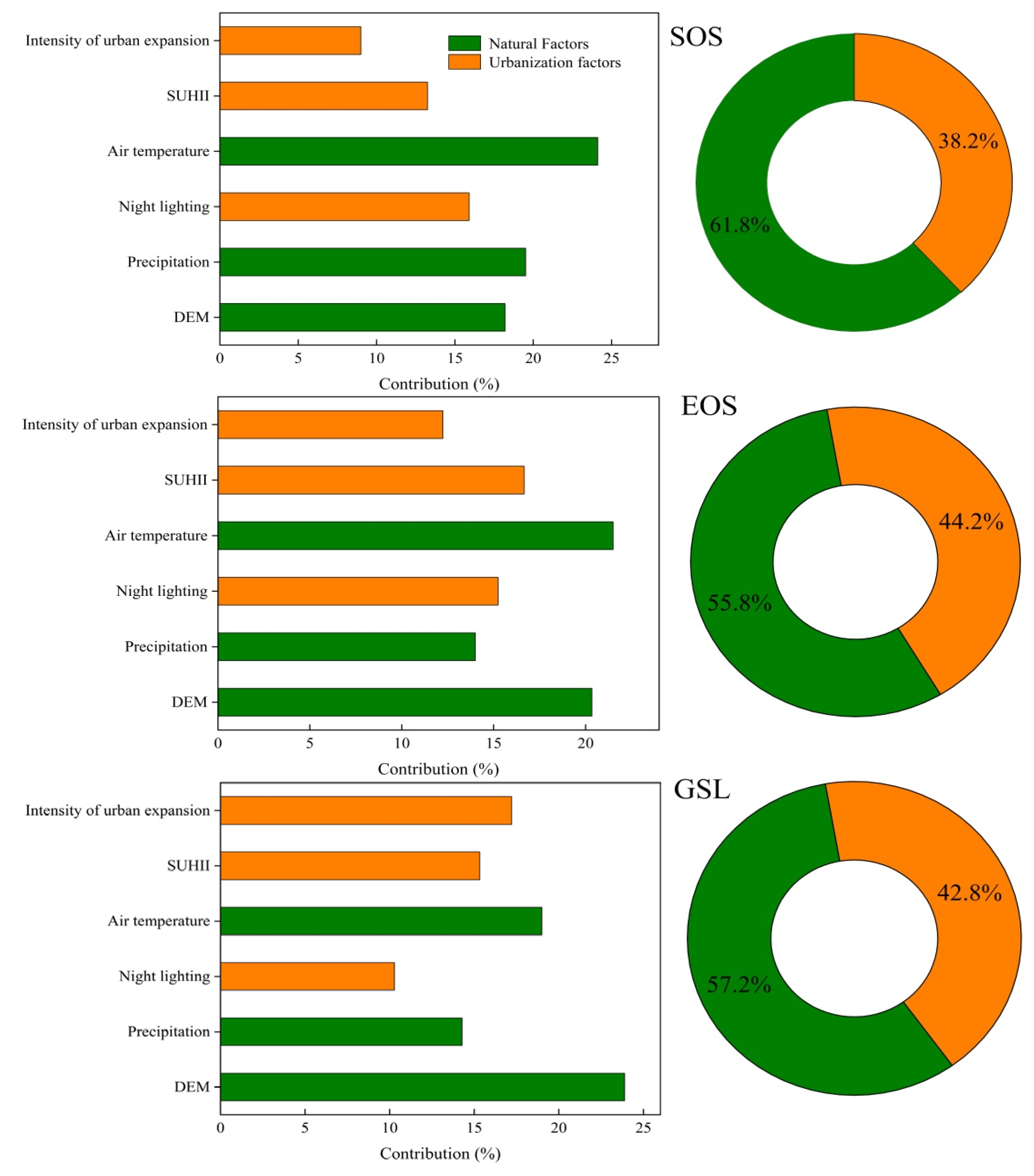
5.2. Contributions of Urbanisation and Natural Factors to Vegetation Phenology

As shown in Figure 13, the influences of urbanisation and natural factors on SOS were 38.2% and 61.8%, respectively, with the largest contribution belonging to the temperature. The urbanisation factor of night-time lighting contributed the most to SOS. The contributions of temperature and night-time lighting to SOS were greater than those of the other factors. The effects of urbanisation and natural factors on EOS were 44.2% and 55.8%, respectively, with the largest contribution belonging to the temperature. The urbanisation factor of SUHII made the largest contribution to EOS. The contributions of temperature and SUHII to EOS were greater than those of the other factors. The effects of urbanisation and natural factors on GSL were 42.8% and 57.2%, respectively, with the DEM and urban expansion intensity being the largest natural and urbanisation contributors, respectively. In general, urbanisation and natural factors contributed considerably to the changes in the vegetation phenology in the study area.

5.3. Uncertainty Analysis

The natural environment and topography of the study area are complex, and many factors affected the SUHII estimation, which may lead to errors in the estimation results. Additionally, the characteristics of the study area differed from those previously reported in related literature, which may make the conclusions drawn from this study differ from those drawn from them. For example, the cold island effect was also present in the UANSTM Zone across a large geographical area. However, the extent of the heat island effect, the focus of this study, was over a small urban-suburban-rural area. Therefore, future studies on the effects of urban cold islands on vegetation phenology should be conducted on a larger scale. The large area of cultivated land around the study area and the vegetation phenology of farmland, which largely depends on crop types and management practises, led to complexity and uncertainty in the detection of farmland phenology. In addition to the factors covered in the present study, urbanisation and natural factors themselves contain more elements; thus, more factors should be considered in the future to quantify their effects on vegetation phenology in the context of urban-rural interactions.

6. Conclusions

  • The vegetation phenological variables in the study area showed pronounced differences across the spatial gradients between urban and rural areas. The closer it was to the urban centre, the earlier the start of the growing season was, the later its end was, and the longer the growing season was. The intensity of the heat island varied significantly among the three urban clusters. The intensity of the SUHII was highest in the Urumqi-Changji region.
  • The heat island effect of the urban agglomerations in the study area influenced the spatiotemporal patterns of the surrounding vegetation phenology; however, there was some variability in the effects of the three urbanisation levels on the surrounding vegetation phenology. The urbanisation level of the urban clusters was negatively correlated with SOS but positively correlated with EOS and GSL. The urbanisation level of the Urumqi-Changji district was high and highly influenced the vegetation phenology. The increased fraction of built-up land area delayed SOS, advanced EOS, and lengthened GSL in urban centres. The SUHII value of the urban cluster was significantly correlated negatively with SOS but highly and positively with ΔEOS and ΔGSL.
  • The temperature effect was slightly stronger on vegetation phenology than the precipitation effect, with the temperature effect on SOS and EOS being highly significant. A close relationship was found between vegetation phenology and altitude, with the GSL showing a significant correlation.
  • The spatiotemporal patterns of the vegetation phenology in the study area along the urban-rural gradient were the product of urbanisation and natural factors. The interactions between urbanisation and natural factors significantly affected the vegetation phenology. The contribution of the urbanisation factors to EOS was 44.2%, and the contribution of the natural factors to SOS was 61.8%.

Author Contributions

All authors contributed substantially to this study. Resources, data curation, validation, visualisation, writing (original draft), and writing (review and editing), G.A. and M.Z.; resources, conceptualisation, supervision, writing (original draft), and writing (review and editing), M.Z.; review and editing, A.K. and P.H. All authors have read and agreed to the published version of the manuscript.

Funding

This research was funded by the Xinjiang Uygur Autonomous Region Key Laboratory Bidding Project (XJDX0909-2021-01), the National Natural Science Foundation Programme (42261013), the Postgraduate Research and Innovation Project of Xinjiang Normal University (grant number XSY202201003), and the Third Xinjiang Scientific Expedition Programme (2021xjkk0905).

Institutional Review Board Statement

Not applicable.

Informed Consent Statement

Not applicable.

Data Availability Statement

The datasets used in this study are available from the corresponding author upon request.

Acknowledgments

The authors thank anonymous reviewers for their constructive comments and suggestions.

Conflicts of Interest

The authors declare no conflict of interest.

References

  1. Richardson, A.D.; Keenan, T.F.; Migliavacca, M.; Ryu, Y.; Sonnentag, O.; Toomey, M. Climate change, phenology, and phenological control of vegetation feedbacks to the climate system. Agric. Forest Meteorol. 2013, 169, 156–173. [Google Scholar] [CrossRef]
  2. Ahmed, G.; Mei, Z.A.N. The influence of heat island effect on vegetation phenology in major urban clusters in the Tianshan Northslope economic belt of Xinjiang. J. Ecol. Rural Environ. 2022, 38, 872–881. [Google Scholar]
  3. Jochner, S.; Heckmann, T.; Becht, M.; Menzel, A. The integration of plant phenology and land use data to create a GIS-assisted bioclimatic characterisation of Bavaria, Germany. Trans. Bot. Soc. Edinb. 2011, 4, 91–101. [Google Scholar] [CrossRef]
  4. Ren, C.; Zhang, T.; Li, R. Response of growing period and phenology duration of herbaceous plants to climate change in Southwestern Shandong Province. Clim. Chang. Res. Lett. 2015, 4, 25–31. [Google Scholar] [CrossRef]
  5. Hu, K.; Guo, Y.; Yang, X.; Zhong, J.; Fei, F.; Chen, F.; Zhao, Q.; Zhang, Y.; Chen, G.; Chen, Q.; et al. Temperature variability and mortality in rural and urban areas in Zhejiang Province, China: An application of a spatiotemporal index. Sci. Total Environ. 2019, 647, 1044–1051. [Google Scholar] [CrossRef]
  6. Forkel, M.; Migliavacca, M.; Thonicke, K.; Reichstein, M.; Schaphoff, S.; Weber, U.; Carvalhais, N. Codominant water control on global interannual variability and trends in land surface phenology and greenness. Glob. Chang. Biol. 2015, 21, 3414–3435. [Google Scholar] [CrossRef]
  7. Piao, S.; Liu, Q.; Chen, A.; Janssens, I.A.; Fu, Y.; Dai, J.; Liu, L.; Lian, X.; Shen, M.; Zhu, X. Plant phenology and global climate change: Current progresses and challenges. Glob. Chang. Biol. 2019, 25, 1922–1940. [Google Scholar] [CrossRef]
  8. Germino, M.J.; Lazarus, B.E. Weed-suppressive bacteria have no effect on exotic or native plants in sagebrush-steppe. Rangel Ecol. Manag. 2020, 73, 756–759. [Google Scholar] [CrossRef]
  9. Roetzer, T.; Wittenzeller, M.; Haeckel, H.; Nekovar, J. Phenology in central Europe-differences and trends of spring phenophases in urban and rural areas. Int. J. Biometeorol. 2000, 44, 60–66. [Google Scholar] [CrossRef]
  10. Zhang, X.; Friedl, M.A.; Schaaf, C.B.; Strahler, A.H. Climate controls on vegetation phenological patterns in northern mid- and high latitudes inferred from MODIS data. Glob. Chang. Biol. 2004, 10, 1133–1145. [Google Scholar] [CrossRef]
  11. Luo, Z.; Sun, O.J.; Ge, Q.; Xu, W.; Zheng, J. Phenological responses of plants to climate change in an urban environment. Ecol. Res. 2007, 22, 507–514. [Google Scholar] [CrossRef]
  12. Ding, H.Y.; Qin, B.Y.; Ming, X.L. Spatial and temporal variation of vegetation phenology in the Yangtze River Delta and its response to urbanization. J. Saf. Environ. 2021, 21, 9. [Google Scholar]
  13. Jeong, S.J.; Park, H.; Ho, C.H.; Kim, J. Impact of urbanization on spring and autumn phenology of deciduous trees in the Seoul Capital Area, South Korea. Int. J. Biometeorol. 2019, 63, 627–637. [Google Scholar] [CrossRef]
  14. Liu, J.-L.; Guo, H.-D.; Lu, Z. Research on the influence of urbanization on vegetation phenology in Beijing-Tianjin-Tangshan area. Remote Sens. Technol. Appl. 2014, 29, 286–292. [Google Scholar]
  15. Zhao, W.Y.; Chen, Y.N.; Li, J.L.; Jia, G.S. Periodicity of plant yield and its response to precipitation in the steppe desert of the tianshan mountains region. J. Arid Environ. 2010, 74, 445–449. [Google Scholar] [CrossRef]
  16. Li, W.-M.; Qin, Z.-H.; Li, W.-J. Comparative analysis of MODIS NDVI and MODIS EVI. Remote Sens. Inf. 2010, 06, 73–78. [Google Scholar]
  17. Qiao, Z.; Tian, G.; Xiao, L. Diurnal and seasonal impacts of urbanization on the urban thermal environment: A case study of Beijing using MODIS data. ISPRS J. Photogramm. 2013, 85, 93–101. [Google Scholar] [CrossRef]
  18. Pongracz, R.; Bartholy, J.; Dezso, Z. Remotely sensed thermal information applied to urban climate analysis. Adv. Space Res. 2006, 37, 2191–2196. [Google Scholar] [CrossRef]
  19. Chen, Z.; Yu, B.; Yang, C.; Zhou, Y.; Yao, S.; Qian, X.; Wang, C.; Wu, B.; Wu, J. An Extended Time-Series. 2000–2018 of Global NPP-VIIRS-Like Nighttime Light Data. Earth Syst. Sci. Data 2020, 13, 889–906. [Google Scholar] [CrossRef]
  20. Liu, Y.H.; Fang, S.Y.; Zhang, S.H. Quantitative assessment of heat islands in the Beijing-Tianjin-Hebei urban agglomeration. J. Ecol. 2017, 37, 18. [Google Scholar]
  21. Han, G.-F.; Xu, J.-H.; Yuan, X.-Z. The impact of urbanization on the vegetation phenology of major cities in the Yangtze River Delta. J. Appl. Ecol. 2008, 08, 1803–1809. [Google Scholar]
  22. Liu, Z.; Zhou, Y.; Feng, Z. Response of vegetation phenology to urbanization in urban agglomeration areas: A dynamic urban-rural gradient perspective. Sci. Total Environ. 2023, 864, 161109. [Google Scholar] [CrossRef] [PubMed]
  23. Moazzam, M.F.U.; Doh, Y.H.; Lee, B.G. Impact of urbanization on land surface temperature and surface urban heat Island using optical remote sensing data: A case study of Jeju Island, Republic of Korea. Build. Environ. 2022, 222, 109368. [Google Scholar] [CrossRef]
  24. Li, G.; Fang, C.; Li, Y.; Wang, Z.; Sun, S.; He, S.; Qi, W.; Bao, C.; Ma, H.; Fan, Y.; et al. Global impacts of future urban expansion on terrestrial vertebrate diversity. Nat. Commun. 2022, 13, 1628. [Google Scholar] [CrossRef] [PubMed]
  25. Yu, W.; Shi, J.; Fang, Y.; Xiang, A.; Li, X.; Hu, C.; Ma, M. Exploration of urbanization characteristics and their effect on the urban thermal environment in Chengdu, China. Build. Environ. 2022, 219, 109150. [Google Scholar] [CrossRef]
  26. van den Heuvel, E.; Zhan, Z. Myths about linear and monotonic associations: Pearson’sr, Spearman’s ρ, and Kendall’s τ. Am. Stat. 2022, 76, 44–52. [Google Scholar] [CrossRef]
  27. Wang, J.F.; Li, X.H.; Christakos, G.; Liao, Y.; Zhang, T.; Gu, X.; Zheng, X. Geographical Detectors-Based Health Risk Assessment and its Application in the Neural Tube Defects Study of the Heshun Region, China. Int. J. Geogr. Inf. Sci. 2010, 24, 107–127. [Google Scholar] [CrossRef]
  28. Zhang, M.; Kafy, A.A.; Ren, B.; Zhang, Y.; Tan, S.; Li, J. Application of the optimal parameter geographic detector model in the identification of influencing factors of ecological quality in Guangzhou, China. Land. 2022, 11, 1303. [Google Scholar] [CrossRef]
  29. Deng, X.; Hu, S.; Zhan, C. Attribution of vegetation coverage change to climate change and human activities based on the geographic detectors in the Yellow River Basin, China. Environ. Sci. Pollut. Res. Int. 2022, 29, 44693–44708. [Google Scholar] [CrossRef]
  30. Dong, Z.Y.; Zhang, Y.S. Analysis of the contribution of land surface temperature based on urban landscape pattern and connectivity. Geogr. Inf. World. 2020, 27, 75–82. [Google Scholar]
  31. Deng, C.; Ma, X.; Xie, M.; Bai, H. Effect of altitude and topography on vegetation phenological changes in the Niubeiliang nature reserve of Qinling Mountains, China. Forests 2022, 13, 1229. [Google Scholar] [CrossRef]
  32. Fan, J.; Min, J.; Yang, Q.; Na, J.; Wang, X. Spatial-temporal relationship analysis of vegetation phenology and meteorological parameters in an agro-pasture ecotone in China. Remote Sens. 2022, 14, 5417. [Google Scholar] [CrossRef]
  33. Yao, R.; Cao, J.; Wang, L.; Zhang, W.; Wu, X. Urbanization effects on vegetation cover in major African cities during 2001. Int. J. Appl. Earth Obs. Geo Inf. 2019, 75, 44–53. [Google Scholar] [CrossRef]
  34. Hu, Z.L.; Dai, H.; Hou, F.; Li, E. Temporal and spatial changes of vegetation phenology in urban and rural areas in Northeast China and its response to surface temperature. Acta Ecol. Sin. 2020, 40, 4137–4145. [Google Scholar]
  35. Zhou, D.; Zhao, S.; Zhang, L.; Liu, S. Remotely sensed assessment of urbanization effects on vegetation phenology in China’s 32 major cities. Remote Sens. Environ. 2016, 176, 272–281. [Google Scholar] [CrossRef]
Figure 1. Land-use and land-cover types and major urban areas in the study area in 2020.
Land 12 01108 g001
Figure 2. Workflow flowchart adopted in the present study.
Land 12 01108 g002
Figure 3. Spatial and temporal patterns of the average start of growing season (SOS), end of growing season (EOS), and growing season length (GSL) in the study area during 2001–2020.
Land 12 01108 g003
Figure 4. Relationships between distance from the city centre and (a) ΔSOS, (b) ΔEOS, and (c) ΔGSL.
Land 12 01108 g004
Figure 5. Spatial patterns of daytime (a) and night-time (b) surface urban heat island intensity (SUHII) in the study area during 2001–2020.
Land 12 01108 g005
Figure 6. Distance from urban centre versus multi-year average values of day (a) and night (b) SUHII.
Land 12 01108 g006
Figure 7. Effects of the three urbanisation levels on the vegetation phenology in the different urban agglomerations: (a) Urumqi-Changji, (b) Shihezi-Manasi, and (c) Wusu-Kuidun-Dushanzi.
Land 12 01108 g007
Figure 8. Relationship between the SUHII and vegetation phenology of (a) ΔSOS, (b) ΔEOS, and (c) ΔGSL along the urban-rural gradient.
Land 12 01108 g008
Figure 9. Correlation between precipitation and (a) SOS, (b) EOS, and (c) GSL in the UANSTM.
Land 12 01108 g009
Figure 10. Correlation between average temperature and (a) SOS, (b) EOS, and (c) GSL in the UANSTM.
Land 12 01108 g010
Figure 11. Changes in the mean vegetation phenology in relation to altitude on the northern slopes of the Tianshan Mountains.
Land 12 01108 g011
Figure 12. Interactions of the urbanisation factors with the natural factors, SOS (a), EOS (b), and GSL (c). Note: x1, x2, x3, x4, x5, and x6 represent the air temperature, night-time lighting, precipitation, DEM, urban sprawl intensity, and SUHII, respectively.
Land 12 01108 g012
Figure 13. Contributions of urbanisation and natural factors to the vegetation phenology.
Land 12 01108 g013
Table 1. Nature of data and sources.
DatasetData SourceData PropertiesData TypeTime Coverage
MCD12Q2GEE500 m/yrGreenup, Dormancy2001–2019
MOD13Q1 250 m/16 dEVI2020
MOD11A2 1 000 m/8 dLST_Day_1 km, LST_Night_1 km2001–2020
Land-use type datasetNational Earth System Science Data Centre (http://www.geodata.cn/, accessed on 5 September 2020)30 mgrassland, cropland, forest land, water, construction land, and bare land2001, 2010, and 2020
DEMGeospatial Data Cloud30 mASTER GDEM V22020
(http://www.gscloud.cn, accessed on 5 April 2023)
Night-time lighting datasetAn extended time-series (2000–2020) of global NPP-VIIRS-like night-time light data (https://doi.org/10.7910/DVN/YGIVCD, accessed on 5 April 2023)500 m2001–2020
Climate DataNational Earth System Science Data Centre (http://www.geodata.cn/, accessed on 5 April 2023)0.0083333° (approx. 1 km)Precipitation, Temperature2001–2020
Vector dataNational Geographic Information Resource Catalogue Service System (http://www.webmap.cn, accessed on 5 April 2023)Shapefile
DEM, digital elevation model; GEE, Google Earth Engine; LST, land surface temperature.
Table 2. Pearson’s correlation coefficients between vegetation phenological period and urban construction land area (%).
City Cluster NameRegionsSOSEOSGSL
Urumqi-Changjiurban centre−0.85 **0.83 **0.81 **
suburban area−0.560.450.56
rural area−0.74 *0.68 *0.57
Shihezi-Manasiurban centre−0.77 *0.69 *0.68 *
suburban area−0.510.520.33
rural area−0.610.63 *0.45
Wusu-Kuidun-Dushanziurban centre−0.82 **0.79 *0.74 **
suburban area−0.610.570.46
rural area−0.63 *0.650.53
* indicates p < 0.05, ** indicates p < 0.01
Table 3. Coefficients of correlation between SUHII and vegetation phenology.
City Cluster NameΔSOS/SUHIIΔEOS/SUHIIΔGSL/SUHII
DayNightDayNightDayNight
Urumqi-Changji−0.87−0.940.980.950.960.98
Shihezi-Manasi−0.92−0.90.890.940.930.95
Wusu-Kuidun-Dushanzi−0.92−0.790.940.790.940.81
Disclaimer/Publisher’s Note: The statements, opinions and data contained in all publications are solely those of the individual author(s) and contributor(s) and not of MDPI and/or the editor(s). MDPI and/or the editor(s) disclaim responsibility for any injury to people or property resulting from any ideas, methods, instructions or products referred to in the content.

