Abstract
Functional data are being used increasingly in recent years and in many environmental sciences, such as hydrology applied to agriculture. This means that the output, instead of a scalar variable represented by a spatial map, is given by a function. Furthermore, in site-specific management, there is a need to delineate the field into management areas depending on the agricultural procedure and on the scale of application. In this paper, an approach based on multivariate geostatistics is illustrated that uses the parameters of Dexter’s water retention model and some soil properties to arrive at a multiscale delineation of an agricultural field in Iran. One hundred geo-referenced soil samples were taken and subjected to various measurements. The volumetric water contents at the different suctions were fitted to Dexter’s model. The estimated curve parameters plus the measurements of the soil variables were transformed into standardized Gaussian variables and the values transformed were subjected to geostatistical cokriging and factorial cokriging procedures. These results show that soil properties (organic carbon, bulk density, saturated hydraulic conductivity and tensile strength of soil aggregates) influence the parameters of Dexter’s model, although to different extents. The thematic maps of both soil properties and water retention curve parameters displayed a varying degree of spatial association that allowed the identification of homogeneous areas within the field. The first regionalized factors (F1) at the scales of 508 m and 3000 m made it possible to provide different delineations of the field into homogeneous areas as a function of scale, characterized by specific physical and hydraulic properties. F1 at a short and long distance could be interpreted as “porosity indicator” and “hydraulic indicator”, respectively. Such type of field delineation proves particularly useful in sustainable irrigation management. This paper emphasizes the importance of taking the spatial scale into account in precision agriculture.
1. Introduction
Agricultural soils are very complex systems that are capable of storing and transmitting air, water, solutes and heat to microorganisms and plants. Soil consists of solid spaces (particles) and voids (pores) that determine its structural characteristics and function. In particular, water transport, which is crucial in controlling the health and productive potential of a plant, occurs through the connected pore spaces, whereas the workability of soils depends on the existence of pores in the form of microcracks. Pore spaces are determined by the size of composite particles that form a hierarchical system [1,2], consisting of various levels: groups of primary particles comprising microaggregates, microaggregate groups comprising aggregates and aggregate groups comprising clods, which are aggregates formed by tillage according to SSSA Soil glossary, or bulk soil. Similarly, the average pore size follows a hierarchical system determined by the size of the soil particles. Therefore, following [3] the total porosity of soil can be said to contain various components: residual, matrix, structural and macro porosity.
The first and last components include pores that are either too small or too large, respectively, that are generally disregarded in experiments aimed at defining optimal soil water management for irrigation purposes. In contrast, the matrix porosity represents the pore space between individual mineral particles in the soil. As groups of mineral particles can combine to form discrete microaggregates, it is also necessary to consider structural porosity, which is the pore space between the microaggregates and between the incipient aggregates. This type of porosity in most soils is largely composed of microcracks, also called ‘elongated transmission pores’ by Pagliai, Vignozzi and Pellegrini [4], which play an important role in transport processes.
Moreover, it is well known that water in pores is not in a free state, but is subject to a matrix potential whose absolute value is called suction. The relationship between suction and pore water content can be described by a function called soil water content retention curve (SWRC) [5], the shape of which depends on different physical and chemical properties of the soil, which are specific to each soil [6]. SWRC contains useful information on pore water content at different suctions and pore size distributions, which characterize the response of the soil to stress conditions, such as saturation or dryness [7]. Therefore, it is clear that knowledge of it cannot be disregarded for sustainable irrigation water management in a spatially variable agricultural field. However, there are many models of SWRC in the literature that have been compared by various authors [8,9]. In particular, Dexter’s model [3] is a double-exponential equation with five adjustable parameters and a bimodal distribution, and each mode is related to either matrix or structural porosity. Compared with the other models, it has the following advantages: all five parameters have a physical meaning related to the different components of porosity; the parameter related to residual porosity is always positive or zero; the five parameters are poorly correlated with each other and can be related to soil properties influencing its hydraulic behaviour.
Dexter’s model parameters together with other relevant properties of agricultural soil can then be treated jointly in a spatial analysis to arrive at a partitioning of the field into homogeneous areas to be subjected to differential irrigation management. The study of the spatial variability of an agricultural field generally requires soil sampling at a finite number of locations. The samples are then subjected to laboratory measurements and these measurements are processed spatially to produce thematic maps. However, in the case discussed above, the interest is not in one or more scalar variables but in a functional variable; i.e., in the modelling of a water retention curve from a set of soil moisture measurements recorded at the same location and corresponding to gradually increasing values of water suction.
Moreover, it is expected that the functional data will exhibit spatial dependence. Several alternative techniques have been developed by different authors [10] to spatially predict continuous curves instead of single-point data for each observation site. These methods first require the application of a parametric or non-parametric smoothing technique (e.g., Dexter’s model or B-spline regression) to convert discrete data into continuous functions; after that, some interpolation technique is applied to predict the whole curve in unsampled locations. These methods have also been used in several areas besides hydrology and agronomy, including meteorology [11] and marine biology.
In this paper, a multivariate geostatistical approach was preferred for the following main reasons. The fitting of a linear model of coregionalization (LMC) allows the modelling of the spatial relationships of Dexter’s retention curve parameters with each other and with the soil properties considered to be particularly influencing water transport. In addition, multivariate geostatistics make it possible to arrive at a delineation of the field in homogeneous areas that is a function of scale [12,13], since the processes governing soil water transport occur over different scales.
The delineation of management zones for precision irrigation is commonly based on statistical clustering, which combines the impacts of different variables operating over different spatial and temporal scales on the hydraulic behaviour of soil [14,15,16,17]. However, these techniques suffer from two main limitations: (1) they do not take into account the generally observed spatial correlation between spatial observations, and (2) they produce a single field partition at an unspecified spatial scale, even if this partition is produced by processes operating at different scales [18].
Therefore, in light of the above considerations, the objective of this study was to define a multivariate geostatistical approach based on SWRC measurements in an agricultural field to predict the whole curve of Dexter’s model at unsampled points and produce a multiscale field delineation in homogeneous areas for site-specific water management.

| Notation Box | |
|---|---|
| KS | Saturated hydraulic conductivity (ms−1) |
| OC | Organic carbon (℅) |
| BD | Bulk density (g cm−3) |
| TS | Tensile strength of soil aggregates (kPa) |
| θr | Asymptote of the equation, which is residual water content (cm3cm−3) |
| A1 | Amount of matrix pore spaces (cm3cm−3) |
| A2 | Amount of structural pore spaces (cm3cm−3) |
| h1 and h2 | Characteristic pore water suctions at which the matrix and structural pore spaces start to empty, respectively (bar) |
2. Materials and Methods
2.1. Study Area and Experimental Site
The experiment was carried out in a 200-ha field at the Dastjerd Research Farm of the College of Agriculture, Bu-Ali Sina University, Hamedan, Iran (35°02′10.46″ N–35°03′39.72″ N and 48°28′21.25″ E–48°30′0.90″ E) in 2019. One hundred disturbed and undisturbed soil samples were collected from 0.10–0.15 m depth at the nodes of a grid with cells of 150 × 150 m2 size and in some areas of 75 × 75 m2 and 37 × 37 m2 size [13] (Figure 1) to increase the number of pairs of samples at shorter distances and to reduce the nugget effect in variogram models, representing the lower limit of estimation precision.
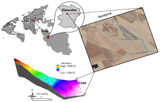
Figure 1.
Location of the study site and sampling points.
The mean annual rainfall is 479.7 mmy−1 and the mean annual temperature is 14.83 °C (daily temperature varying from −9 °C to 35 °C).
2.2. Dexter’s Soil Water Retention Curve (Dexter’s Model)
Soil water content was measured in the undisturbed core samples at the matric potentials of −0.01, −0.02, −0.04 and −0.06 (with a Sandbox apparatus), and −0.3, −1, −5 and −15 bar (with a pressure plate apparatus).
Dexter’s model (Dexter et al., 2008) was fitted to data:
where, w (cm3cm−3): volumetric moisture content of the soil; θr: asymptote of the equation, which is the residual water content (cm3cm−3); A1 (cm3cm−3): amount of matrix pore spaces; A2 (cm3cm−3): amount of structural pore spaces; h (bar): matric suction corresponding to w; h1 (bar) and h2 (bar); characteristic pore water suctions at which the matrix and structural pore spaces start to empty, respectively [3].
Model Fitting
Dexter’s model parameters were estimated using the Excel Solver (2016). To test the goodness of fitting, root mean square error (RMSE) and determination coefficient (R2) were used as follows:
where, N is the number of samples; Yi and Ypi are the measured and predicted values of the variable at location i, respectively.
2.3. Soil Property Measurements
Disturbed soil samples (2 kg) were air-dried and passed through a 2 mm sieve before physical and chemical analyses (Table 1).
Table 1.
Method of measuring study variables.
Table 1.
Method of measuring study variables.
| Variable | Measurement Method | Unit | References |
|---|---|---|---|
| Soil organic carbon (OC) | oxidation method | (%) | [19] |
| Bulk density (BD) | standard core method | (gcm−3) | [20] |
| Saturated hydraulic conductivity (KS) | The constant head method | (ms−1) | [21] |
The studied soils covered five textural classes according to the USDA soil classification (Figure 2) [13]. Soil samples included the following classes: clay loam (n = 6), loam (n = 10), sandy clay loam (n = 57), sandy loam (n = 22) and loamy sand (n = 5).
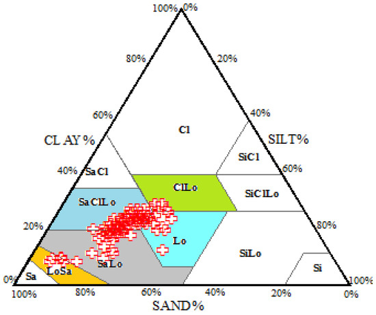
Figure 2.
Distribution of soil texture classes in the United States Department of Agriculture (USDA) textural triangle.
2.4. Aggregate Tensile Strength Measurement
According to Dexter and Kroesbergen (1985), tensile strength is probably the most useful measure of the strength of individual soil aggregates, where soil strength is intended to the highest stress that any type of soil can be exposed to before failure [22]. It is influenced by soil moisture, the degree of connection among soil aggregates and the occurrence of soil cracks [23]. An increase in soil moisture causes a decrease in the bonding strength between the organic and inorganic particles in soil aggregates and a reduction in the tensile strength of soil aggregates [24]. Therefore, given the close relationship between the soil water content and tensile strength, it was decided to include this soil property among the variables chosen for the delineation of soil in hydraulically homogeneous areas. To measure tensile strength, air-dried aggregates with a diameter of 4 to 8 mm were used (Figure 3).
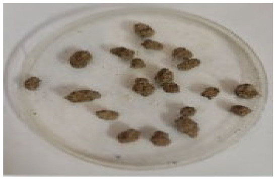
Figure 3.
Soil aggregates.
The reason for using these diameters was the ease of collection and measurement with the available devices. First, twenty aggregates were randomly selected from each soil sample; second, the device described by Dexter and Watts [25] was used to measure the tensile strength (Figure 4). In this device, soil aggregates were placed between the two disks, and pressure was applied to them by adding water to a water container and using a leverage system. Before starting the test, the disk and container were levelled so that no pressure was applied to the aggregates. Pressure was then applied to the aggregates until they broke, at which point the water uptake stopped.
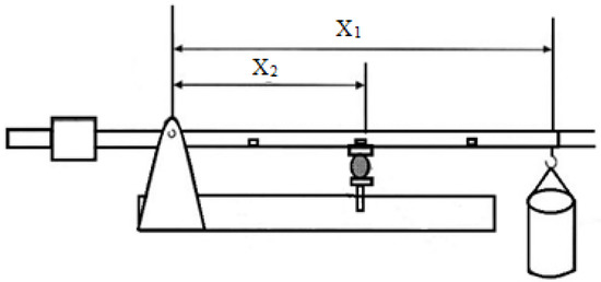
Figure 4.
The device used to measure the force required for breaking soil aggregates [25].
The force (F) in Newton (N) required to break aggregates was calculated using the following equation:
where, Mc is the mass of water (kg) required to break soil aggregates; X1 is the length of the upper lever; X2 is the length of the lower lever (cm); g is gravity acceleration (9.807 ms–2).
Finally, the tensile strength of aggregates was calculated using the following equation based on the method by Rogowski [26] and Dexter and Kroesbergen [27]:
where, Y is tensile strength (kPa); F is the maximum force (N) required for aggregate breaking; deff is the effective diameter of the aggregates assumed to be of spherical shape, which was calculated using the following equation:
dmax and dmin are the maximum and minimum diameters of soil aggregates.
2.5. Multivariate Geostatistical Analysis
The proposed multivariate geostatistical approach jointly treats two different types of data (data fusion): point data concerning the measurements of some soil properties (KS, BD, OC and TS), which were considered to be influencing the hydraulic characteristics of soils, and functional data for the determination of the parameters of Dexter’s model. The objective of such an analysis is two-fold: (1) to determine SWRC at an unsampled point in the field; (2) to characterize the field from a hydraulic point of view to arrive at a partition into homogeneous areas to be subjected to differential irrigation water management.
The approach consists of different steps as follows:
- Fitting of Dexter’s model to determine its five parameters;
- Basic statistics of all study variables including Dexter’s model parameters and the selected soil properties;
- Normalization and standardization of all variables through Gaussian anamorphosis, if they show significant deviations from symmetrical data distribution;
- Fitting of a linear model of coregionalization (LMC) to the whole data set of the experimental direct and cross-variograms of the Gaussian transformed variables to model the spatial relationships of the curve parameters with each other and with soil properties;
- Testing the goodness of fitting through cross-validation;
- Ordinary cokriging on all Gaussian transformed variables and back transformation of the estimates of Gaussian transformed parameters using the anamorphosis Gaussian function previously determined;
- Mapping of soil properties for characterizing spatial variability, and of the curve parameters to draw SWRC in any point of the field;
- Factorial cokriging on Gaussian transformed variables and extraction of the regionalized factors at short and long ranges;
- Mapping of the retained regionalized factors at each scale with eigenvalue greater than 1, which cumulatively explains a good proportion of the spatial variability at that scale;
- Delineation of within-field zones with different hydraulic properties by using the retained regionalized factors.
With regard to the geostatistical procedures used, the interested reader can refer to one of the many published manuals [28] for a detailed description. Only the main steps are briefly described below (Figure 5).
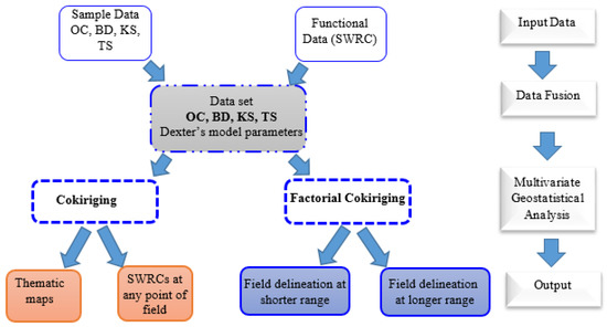
Figure 5.
Flowchart illustrating the methodology followed. All results are described according to this scheme.
2.5.1. Basic Statistics and Gaussian Anamorphosis
The maximum, minimum, mean and median values, standard deviation (SD), skewness and kurtosis were calculated for all study variables to characterize the type of data distribution. In the case of skewed variables, Gaussian anamorphosis was performed to determine a continuous mathematical function that transformed a standardized Gaussian variable into a random variable [29]. For such a transformation, Hermite’s ortho-normal polynomial series was truncated to the first 100 terms.
2.5.2. Spatial Interpolation
- Linear Model of Coregionalization
The LMC represents a simplified model of multiscale spatial relations in a multivariate data set [30,31,32]. It assumes that all direct and cross semi-variograms can be described by the same set of basic spatial structures (standardized semivariograms with unit sill) for each spatial scale (range). What differentiates variables or pairs of variables is only the partial sill of each spatial structure corresponding to a specific scale. Although quite crude, this model nevertheless works well under many experimental conditions [30] since it is based on the assumption that the variables are different manifestations of the same processes operating over different scales in the system under study. Cokriging and Factorial cokriging are two of the standard multivariate geostatistical techniques using the same LMC.
- Factorial Cokriging Analysis
Factorial cokriging analysis (FCA) is a technique very similar to the principal component analysis (PCA) of traditional statistics. The fundamental difference is that instead of being applied to the variance-covariance matrix, it is applied to each coregionization matrix of a given spatial scale and derived from the LMC. The latter can be considered as a variance-covariance matrix, but specific to a given spatial scale. As in PCA, orthonormal components can be extracted, which in geostatistics are called regionalized factors and are scale-dependent. From the loading coefficient values, it is then possible to attribute a particular physical meaning to each factor, which can be regarded as a synthetic indicator of spatial variability. All geostatistical analyses were performed using the Isatis geostatistical software package [33].
- Cross-validation
The quality of the LMC can be evaluated using cross-validation [34], which consists of removing one observation at a time and then producing the estimate at the point where the observation was removed with the remaining observations. The difference between the estimate and the observation represents the error. Repeating the procedure for all n observations yields n errors for which different statistics can be calculated.
In particular, the mean error (ME), root mean square error (RMSE) and root mean square standardized error (RMSSE) were calculated using the following equations:
where, n is the number of samples; (xi) and z (xi) are the predicted and measured values of the variable at point xi, respectively; is the root mean squared prediction error. The optimal values for ME and RMSE should be 0, whereas RMSSE should be close to one within the heuristic tolerance interval [35].
3. Results and Discussion
3.1. Basic Statistics of Soil Properties
The basic statistics of the soil properties are presented in Table 2. Related to variations in soil texture [13] and structure (Table 2), 40% of the soil samples had a very high KS (>0.12 m/h), 23% had high KS (0.06–0.12 m/h), 29% had moderate KS (0.02–0.06 m/h), 4% had low KS (0.01–0.02 m/h) and 4% had very low KS (<0.01 m/h) [36]. For low KS, runoff is quite irregular and soil may be suitable for irrigation [36], whereas for very high KS, (about 40% of soil samples), if soil is used for effluent or waste disposal, possible problems might arise due to potential groundwater contamination. Only 8.9% of soil samples had high BD (1.6–1.7 gcm−3), whereas the others had medium BD (1.3–1.6 gcm−3) [26]; therefore, the permeability of the soil does not cause water runoff or irrigation problems, at least in most circumstances. The box plots reveal the existence of some outliers in the soil properties, with the exception of TS (Figure 6). Strong positive skewness and kurtosis > 3 were observed for KS; however, all variables showed non-symmetrical data distribution.
Table 2.
Basic statistics of soil properties.
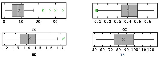
Figure 6.
Box plots of soil variables with outliers (green stars), middle value (vertical line) and mean value (X).
3.2. Basic Statistics of Dexter’s Water Retention Curve Model (SWRC)
The goodness of fitting for the SWRC function to Dexter’s model was satisfactory at any location with an average RMSE of 0.010 (range: 0.001–0.08) and R2 varying between 0.96 and 0.99. The values of model parameters showed general wide variability due to the heterogeneity of soils belonging to different texture classes (Figure 2). High skewness in absolute values (>0.5) was observed in A2 and h2, indicating markedly non-symmetrical data distribution of these parameters (Table 3).
Table 3.
Basic statistics of Dexter’s model parameters.
The box plots (Figure 7) show the presence of outliers only for A2 and h2, which confirms the high asymmetry of the data distribution of these parameters as already indicated by the skewness coefficient.
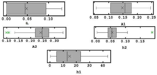
Figure 7.
Box plots with outliers (green stars) of Dexter’s model parameters.
Although the geostatistics estimator is not parametric and, in theory, can be applied to any type of data distribution, variogram modelling is facilitated on Gaussian transformed data. Furthermore, it is also possible to calculate the uncertainty of strongly skewed data [37]. Therefore, before using multivariate analysis, it was preferred to normalize and standardize to zero mean and unit variance for all data (including soil properties and model parameters) due to the presence of skewed variables and outliers.
3.3. Correlation Analysis
In order to detect significant linear correlations between the model parameters and the investigated soil properties, Pearson coefficients were calculated for all variables (Table 4).
Table 4.
Correlation coefficients (r) between the study variables.
A1 and A2 showed significant and positive correlations with OC (0.29 **), while A2 had a negative correlation with BD (−0.38 **). These results are expected because organic carbon is effective in increasing the porosity at the pore sizes investigated and decreasing the bulk density. However, BD seems to be more influenced by structural porosity than by matrix porosity, at least according to Dexter’s model. h1 was negatively correlated with KS (r = −0.22 **), which reflects the fact that high matrix pore water suction has a negative impact on KS. With regard to the relationships between the model parameters, it is worth emphasizing the negative correlation of θr with A1 and h1 and partly with h2, which shows that soils with a high proportion of residual water have a low proportion of matrix pores. Additionally, other significant observations are as follows: the positive correlation between A1 and h1 (0.60 **); the higher the pore water suction at which the matrix pore spaces starts to empty, the higher the proportion of matrix pores; the positive correlation (0.40 **) between the two suctions related to the two sizes of pores. Concerning the significant correlations between soil properties, the positive correlation (0.23 *) of OC with TS is explained because OC increases the soil’s resistance to being crushed. Saturated hydraulic conductivity and OC were negatively correlated with BD (−0.29 **), which was as expected because OC increases porosity, improves KS and reduces BD [38].
It can be deduced from the above results that, although some correlations are significant, there are no strong relationships between the investigated soil properties and the parameters of Dexter’s model. However, these are linear correlations that do not take into account the spatial correlations of the observations. The spatial analysis could confirm these results.
An isotropic LMC was fitted to the matrix of both the direct and cross-experimental variograms of all Gaussian transformed variables, including the following basic spatial structures: (S0) nugget effect, (S1) spherical model (range = 508.64 m) and (S2) spherical model (range = 3000 m) (Figure 8a,b). The proportions of the total spatial variance explained by each spatial component were as follows: S0 50%, S1 13% and S2 37%, which shows that most spatial variation is due to the nugget effect, i.e., spatially uncorrelated error. One way to reduce this spatial component might be to intensify sampling because at the scale at which it was performed, it proved incapable of resolving micro-variability due to both intrinsic soil properties and anthropogenic activities.
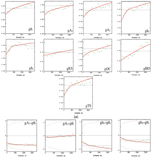

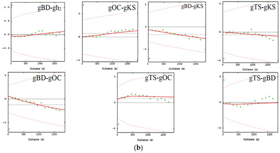
Figure 8.
Experimental direct (a) and cross (b) variograms of the Gaussian transformed variables (points) and the variogram models (bold line). The dashed line indicates an intrinsic (maximum) spatial correlation between the two variables (Wackernagel, 2003). g before the name of variable stands for Gaussian transformed variable.
From Figure 8a of the LMC, some considerations can be made as follows: all direct variograms show a high nugget, as already noted in general above, which can be attributed to the adopted sampling scale, which should be reduced, as well as the measurement error associated with the measurement of soil properties and parameter estimation error. In addition, all direct variograms clearly show a short-range structure (around 500 m), which can be attributed to intrinsic soil variation within the field and the effects of anthropogenic operations, and a long-range structure (around 3000 m), causing the sill to exceed the sampling variance, which can be attributed to the study area belonging to soil map units extending beyond the field size [13]. Deviating from the characteristics stated above, there is a KS variogram, which is similar to the pure nugget effect, most likely determined by the low precision of its measurement marked by high stochasticity; and that of BD, in which the long-range component prevails since BD is generally closely linked to the type of map unit to which the soil belongs at a scale greater than that of the field (Figure 8a).
Regarding the cross-variograms between the model parameters and soil properties, it can be said that in general the spatial relationships are quite low. This can be ascertained from the large distance of the model curve of the cross-variograms from the dashed line (Figure 8b) representing the intrinsic correlation, i.e., the maximum obtainable spatial correlation between the two variables considered [32]. The only soil properties that show spatial correlations of some significance with the model parameters are OC, which is positive with A1 and A2 due to the positive effect already noted for OC on both matrix and structural porosity; and BD, which is negative with θr and A2 but positive with h1, meaning that an increase in density causes a reduction in structural porosity and the amount of residual water, but an increase in the suction at which matrix pores become empty. Regarding the spatial relationships between the various parameters of the model, from the cross-variograms, it can be seen that θr is negatively correlated with all but A2; A1 is positively correlated with h1 and, to a lesser extent, with h2. It is noteworthy that A1 and A2 are not significantly correlated; that is, there is no significant spatial relationship between the two types of porosity (Figure 8b). This is probably attributable to the different origins of the two types of porosity; A1 (matric porosity) is intrinsically linked to the granulometric characteristics of the soil (texture), whereas A2 (structural porosity) is mostly related to the type of tillage carried out in the field. Moreover, A2, similarly to the other parameters of Dexter’s model, shows a high degree of stochasticity (nugget effect) and is the one that appears least correlated with the other parameters (Figure 8b).
There is a positive relationship between h1 and h2 and between h1 and A1; therefore, higher porosity, at least matrix porosity, is associated with higher suction, at which pores (of both types) begin to empty.
Finally, with regard to the spatial relationships among the soil properties investigated, KS appears to be poorly correlated with all of them, mostly due to its essentially stochastic nature. It shows a slight negative correlation with BD, which is quite expected since the densest soils are those with the lowest porosity and, therefore, with low hydraulic conductivity. TS is spatially uncorrelated with the other soil properties, except for a somewhat positive correlation with OC. Therefore, it can be said that both of these properties (OC and TS) contributed to improving the soil structure and consequently its hydraulic characteristics.
Summarising the previous results concerning (1) the high nugget effect for direct variograms, and (2) the general low sill of cross-variograms, denoting low spatial correlation between the curve parameters and between these and the soil variables, it can be stated that this is attributable to two main causes. The first is related to the insufficient sampling density, as already noted; the second is to the uncertainty inherent in the measurements of the soil variables (especially KS) and to the fact that the parameters of Dexter’s model are not directly measurable physical variables but are estimated parameters with an estimation error that may also be high. However, despite the imprecision associated with the measurement and estimation procedures, we believe that it is possible to disclose interesting spatial relationships among variables related to the soil’s capability of transmitting water.
The goodness of fit of the LMC for any Gaussian transformed variable was evaluated through cross-validation, and the results are shown in Table 5. The ME and RMSE were quite close to 0, and the RMSSE fell within the tolerance interval [0.58–1.42] for all variables.
Table 5.
Results of cross-validation of the studied variables.
The maps of soil attributes display that higher KS and OC values were localized in the central parts of the field, whereas lower values were in the south and south eastern corner (Figure 9a,b). Thus, the OC and KS showed a positive degree of association, and their higher values were associated with higher clay contents as reported elsewhere [13].
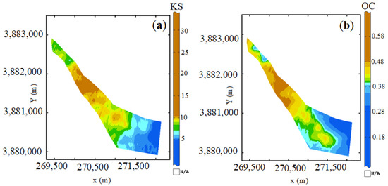
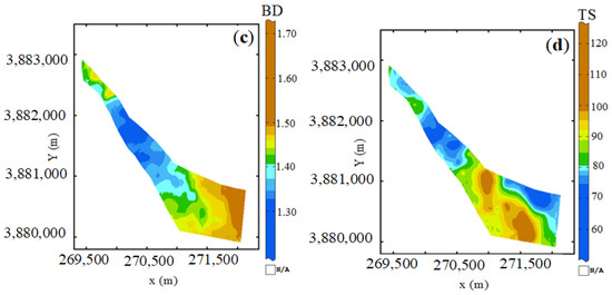
Figure 9.
Cokriging maps of KS (a), OC (b), BD (c) and TS (d). An isofrequency colour scale was used.
Conversely, BD was higher in the southeastern part of the field, where the soils were mostly sandy (Figure 9c) [13]. In the north and central parts, the presence of more OC enhanced the formation of larger soil pores, which reduced BD and improved permeability. Very low KS (0.05–1 cm/h) in the south part of the field, which might cause regular runoff under rainfall and irrigation, is likely to be inefficient. In contrast, in the central part of the field and the north, with hydraulic conductivity greater than 6 mm per hour, superficial water flow would rarely occur, and the soil might be too permeable for irrigation [36].
The aggregate tensile strength map showed a different trend in the field, which is more similar to that of BD (Figure 9d). The lowest values of TS were observed in the central and southeastern parts of the field, probably due to an increase in OC, which might decrease the tensile strength because it might increase the size of the aggregates [39]. Smaller aggregates are stronger because they contain fewer surface cracks [40] and are denser [2]. However, the relationship between OC and TS is not always so direct as it appears to be reversed in some southern parts of the field. This would induce one to think that the resistance of aggregates to the disintegrating action of water actually depended on multiple interrelated factors.
The increase in sand in the southeastern part [13] reduced the tensile strength of aggregates, probably because sand acted as the main nucleus to connect the particles to each other and form larger aggregates, which were more unstable, thereby causing soil fragility to increase [41].
Greater θr values were localized in the central part of the field, whereas smaller values of these parameters were observed in the north and south (Figure 10a). Moisture retention at greater suctions (θr) strongly depends on the particle size distribution [42]; therefore, a finer texture in the central part of the field might have caused an increase in θr.
Figure 10.
Cokriging maps of θr (a), A1 (b), A2 (c), h1 (d) and h2 (e). An isofrequency colour scale was used.
A1 showed the lowest values in the southern part of the field, whereas the highest values were observed in the central and northern parts of the field, probably due to the silt content, which is mostly responsible for the pores of the soil matrix [43]. A2 map shows a very similar pattern to A1 map with the exception of the northern part, where the structural porosity is reduced (Figure 10c) due, as already noted, to the higher silt content in soils to the north. However, throughout the field, the proportion of structural pores prevails over that of matrix pores; that is, the larger pores between the soil aggregates can favour water flow and avoid water logging.
However, a correct proportion between macro- and micro-porosity is fundamental for rational water management in an agricultural field because, while the former facilitates water flow and avoids waterlogging, the latter increases water availability to crops. This critical balance can be achieved by adopting, for example, conservation agriculture techniques [44] that improve the sustainable use of water resources. The higher OC content in the central part has a positive effect, especially on structural pores (A2, Figure 10c), which improves the hydraulic properties and, in particular, promotes the water flow near soil-saturated conditions (KS, Figure 9a). Therefore, from the above discussion, the central part seems to have water characteristics that make it suitable for irrigation. In contrast, the greater values of sand and BD (smaller values of total porosity) in the southern part of the field would have caused a loss of structural and matrix porosity, which explains the reduction in A1 and A2. Therefore, the plants in this part of the field might be more frequently susceptible to water stress than elsewhere.
The maps of h1 and h2 (Figure 10d,e) show a somewhat opposite trend to that of A1 and A2, whereby greater (both structural and matrix) porosity generally corresponds to lower suctions. The highest values of h1 and h2 are observed in the south, with larger contents of sand. However, the relationship between porosity and suction is not so direct and is greatly influenced by the variations in texture and pore size variation spectra that occur in the field. For example, loam sandy soils (sands and sandstones) located in the northeast and southwest have a very narrow distribution of pore sizes; therefore, they empty over a very narrow range of suctions [45]. Furthermore, tillage management can affect porosity and suction at which pores become empty because soils under conventional tillage produce higher structural porosity (large and medium pores) and lower matrix porosity (small pores) than soils under no tillage or conservative agriculture [46,47], thus reducing the risk of water stress. Therefore, more conservative and less energy-demanding techniques should be promoted, as the field was only subjected to conventional tillage at least until the sampling date.
The maps in Figure 9 can also be used to derive SWRC curves at each point in the field. As an example, the curves at three locations in the field (Figure 9a) that clearly differed in their hydraulic properties, as discussed above, are shown (Figure 9a).
The hydraulic differences among the three zones are also well shown by the SWRC curves; in fact, at equal suction, the highest values of water content occur in the middle zone, the lowest in the southeast zone and the intermediate in the north zone (Figure 11a). These variations, as discussed above, can clearly be interpreted in terms of textural variations (higher content of silt in the north, clay in the center and sand in the south-east) and OC (higher content in the central zone), which have an impact on bulk density and porosity and, thus, on water availability to plants.
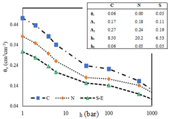
Figure 11.
Estimated SWRC curves for three zones of the field. C: Center; N: North; S: South.
3.4. Factorial Cokriging
To synthesize the spatial relationships shown above between Dexter’s model parameters and soil properties, and simultaneously arrive at a delineation of the field into hydraulically homogeneous areas, a factor analysis was carried out. Only the first factor (F1 short) at the shorter range (508.64 m) and the first and second factors (F1 long and F2 long) at a longer range (3000 m) were retained, with eigenvalues greater than 1, thereby explaining a larger percentage of the variance than that explained by each variable standardized to variance 1. The percentages of spatial variance at the corresponding scale explained by F1 short, F1 long and F2 long were 73.72%, 68.79% and 24%, respectively (Table 6).
Table 6.
Composition of the retained regionalized factors at the scales of 508.64 m and 3000 m.
On F1 short, the Gaussian variables were as follows: gh1, gh2, gTS and gOC, and to a less extent gA1 and gA2 weigh negatively, whereas gθr weighs positively. Therefore, this factor may be considered an indirect “porosity indicator” associated with higher values of OC and TS. It is worth underlining that, at this scale, the porosities and suctions of both types are positively correlated. Therefore, low values of F1 short are an indicator of soils with high total porosity, greater content of OC, more stable aggregates and low content of residual water. On F1 long, gOC, gA2, gKS and gθr weigh more and positively,, whereas BD weighs negatively, as expected. Therefore, at this scale, the structural porosity and the content of OC significantly affect the flow of water in the soil. This factor can then be considered a direct “hydraulic indicator” of the properties of the soil. F2 long, although it explains only 24% of the variance at a 3000 m scale, it was nevertheless retained because it can be assumed as an indirect “aggregate stability indicator”, as TS weighs much more negatively than the other variables (Table 6).
Therefore, from the composition of the retained factors, it is evident how the relationships between the variables change depending on the scale, as they are linked to processes that occur in the soil over different scales [12]. It is, therefore, expected that the maps of the three factors also have a different pattern and, thus, produce a different partition of the field into homogeneous areas. To stress the differences among the structures of spatial dependence, three classes of equal frequency, i.e., of the same spatial extension, were used, which could be defined as follows: low, medium and high classes of total porosity, water flow and aggregate stability for F1 short, F1 long and F2 long, respectively, taking into account the particular composition of these regionalized factors (Figure 12).
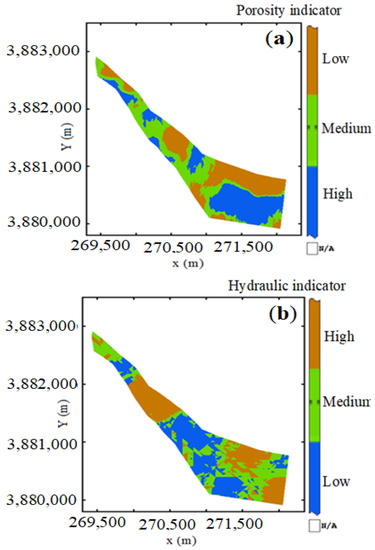
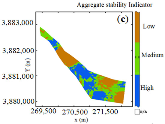
Figure 12.
Maps of porosity indicator (a), hydraulic indicator (b) and aggregate stability indicator (c).
The F1 short map (Figure 12a) appears to be divided into several micro-areas characterized by different porosity and consequent permeability, and aggregate stability, to be associated with local variations in texture and OC, but without a clear overall trend. The high areas are those particularly suited to mechanical tillage and irrigation (especially the wide blue coloured area in the south).
The geometric pattern changes markedly in the map of F1 long, in which one can recognize a large central zone, which also extends partly to the south in a narrower form, characterized by good water flow conditions favored by high structural porosity. These properties, determined by pedological characteristics and higher OC content at a longer scale, should reduce the risk of flooding or waterlogging in the occurrence of extreme weather events.
The map of F2 long (Figure 12c) also appears rather fragmented, as shown in Figure 11a, with numerous areas characterized by higher aggregate stability, which improves resistance to the destructive action of water, extending from the center of the field towards the south (blue coloured areas). Summarizing the above, it is evident that there is no single partition of the field into homogeneous areas based on the hydraulic properties, but this depends significantly on the scale. Nevertheless, it can be said that there is a large central zone, which is more suitable for irrigation, whereas the northern and southern zones are more variable. In particular, the southern zone with a coarser texture might cause problems for irrigation, so it would be advisable to intervene with smaller but more frequent irrigation volumes and more substantial organic fertilization.
4. Conclusions
In this paper, a particular approach based on multivariate geostatistics is proposed in order to jointly process (data fusion) two types of data: soil properties by point-based measurements and functional data to determine the parameters of Dexter’s model of the SWRC curve. This model was chosen among many because its parameters have physical meaning to be associated with the hydraulic properties of the soil. This approach proved effective in interpolating functional data and in rendering scale-dependent field delineation. However, this study highlights two issues. First, the scale of sampling should be appropriate for the observed variability. An excessively high nugget, which prevails over the other structured spatial components, is indicative of the need to intensify sampling by reducing its scale.
Second, there is no single partitioning of the field into homogeneous areas to be subjected to differential management; instead, it is a function of scale. Therefore, it is critical to determine which agronomic procedure is to be optimized and to investigate the scale of the processes involved. Unfortunately, there are few scientific works that have produced a partitioning of an agricultural field according to scale, whereas this crucial topic would require a more widespread and detailed treatment in precision agriculture.
Author Contributions
Conceptualization, A.C. and L.H.; methodology, A.C., L.H. and H.B.; software, A.C.; formal analysis, A.C. and L.H.; data curation, L.H.; writing—original draft preparation, A.C.; writing—review and editing, A.C., L.H. and H.B.; supervision, H.B.; project administration, H.B.; funding acquisition, H.B. All authors have read and agreed to the published version of the manuscript.
Funding
This work was funded by the Bu-Ali Sina University, Hamedan, Iran. Also, this research was partially supported by Iran National Science Foundation (INSF).
Data Availability Statement
Data are contained within the article.
Conflicts of Interest
The authors declare no conflict of interest.
References
- Hadas, A. Long-term tillage practice effects on soil aggregation modes and strength. Soil Sci. Soc. Am. J. 1987, 51, 191–197. [Google Scholar] [CrossRef]
- Dexter, A.R. Advances in characterization of soil structure. Soil Tillage Res. 1988, 11, 199–238. [Google Scholar] [CrossRef]
- Dexter, A.; Richard, G.; Arrouays, D.; Czyż, E.; Jolivet, C.; Duval, O. Complexed organic matter controls soil physical properties. Geoderma 2008, 144, 620–627. [Google Scholar] [CrossRef]
- Pagliai, M.; Vignozzi, N.; Pellegrini, S. Soil structure and the effect of management practices. Soil Tillage Res. 2004, 79, 131–143. [Google Scholar] [CrossRef]
- Jury, W.A.; Horton, R. Soil Physics; John Wiley & Sons: Hoboken, NJ, USA, 2004. [Google Scholar]
- Botula, Y.-D.; Cornelis, W.; Baert, G.; Van Ranst, E. Evaluation of pedotransfer functions for predicting water retention of soils in Lower Congo (DR Congo). Agric. Water Manag. 2012, 111, 1–10. [Google Scholar] [CrossRef]
- Fredlund, M.D.; Wilson, G.W.; Fredlund, D.G. Use of the grain-size distribution for estimation of the soil-water characteristic curve. Can. Geotech. J. 2002, 39, 1103–1117. [Google Scholar] [CrossRef]
- Omuto, C.; Gumbe, L. Estimating water infiltration and retention characteristics using a computer program in R. Comput. Geosci. 2009, 35, 579–585. [Google Scholar] [CrossRef]
- Ebrahimi, E.; Bayat, H.; Neyshaburi, M.R.; Zare Abyaneh, H. Prediction capability of different soil water retention curve models using artificial neural networks. Arch. Agron. Soil Sci. 2014, 60, 859–879. [Google Scholar] [CrossRef]
- Giraldo, R.; Dabo-Niang, S.; Martinez, S. Statistical modeling of spatial big data: An approach from a functional data analysis perspective. Stat. Probab. Lett. 2018, 136, 126–129. [Google Scholar] [CrossRef]
- Giraldo, R.; Delicado, P.; Mateu, J. Continuous time-varying kriging for spatial prediction of functional data: An environmental application. J. Agric. Biol. Environ. Stat. 2010, 15, 66–82. [Google Scholar] [CrossRef]
- Belmonte, A.; Gadaleta, G.; Castrignanò, A. Use of Geostatistics for Multi-Scale Spatial Modeling of Xylella fastidiosa subsp. pauca (Xfp) Infection with Unmanned Aerial Vehicle Image. Remote Sens. 2023, 15, 656. [Google Scholar] [CrossRef]
- Heydari, L.; Bayat, H.; Castrignanò, A. Scale-dependent geostatistical modelling of crop-soil relationships in view of Precision Agriculture. Precis. Agric. 2023, 24, 1–27. [Google Scholar] [CrossRef]
- Cohen, S.; Cohen, Y.; Alchanatis, V.; Levi, O. Combining spectral and spatial information from aerial hyperspectral images for delineating homogenous management zones. Biosyst. Eng. 2013, 114, 435–443. [Google Scholar] [CrossRef]
- Johnson, C.K.; Mortensen, D.A.; Wienhold, B.J.; Shanahan, J.F.; Doran, J.W. Site-specific management zones based on soil electrical conductivity in a semiarid cropping system. Agron. J. 2003, 95, 303–315. [Google Scholar] [CrossRef]
- Peralta, N.R.; Costa, J.L.; Balzarini, M.; Angelini, H. Delineation of management zones with measurements of soil apparent electrical conductivity in the southeastern pampas. Can. J. Soil Sci. 2013, 93, 205–218. [Google Scholar] [CrossRef]
- Yari, A.; Madramootoo, C.A.; Woods, S.A.; Adamchuk, V.I.; Huang, H.-H. Assessment of field spatial and temporal variabilities to delineate site-specific management zones for variable-rate irrigation. J. Irrig. Drain. Eng. 2017, 143, 04017037. [Google Scholar] [CrossRef]
- Reyes, J.; Wendroth, O.; Matocha, C.; Zhu, J.; Ren, W.; Karathanasis, A. Reliably mapping clay content coregionalized with electrical conductivity. Soil Sci. Soc. Am. J. 2018, 82, 578–592. [Google Scholar] [CrossRef]
- Walkley, A.; Black, I.A. An examination of the Degtjareff method for determining soil organic matter, and a proposed modification of the chromic acid titration method. Soil Sci. 1934, 37, 29–38. [Google Scholar] [CrossRef]
- Grossman, R.; Reinsch, T. 2.1 Bulk density and linear extensibility. In Methods of Soil Analysis: Part 4 Physical Methods; Soil Science Society of America, Inc.: Madison, WI, USA, 2002; Volume 5, pp. 201–228. [Google Scholar]
- Klute, A.; Dirksen, C. Hydraulic conductivity and diff usivity: Laboratory methods. In Methods of Soil Analysis, 2nd ed.; ASA: Madison, WI, USA, 1986; pp. 687–732. [Google Scholar]
- Hillel, D. Fundamentals of Soil Physics; Academic Press: New York, NY, USA, 1980. [Google Scholar]
- Kay, B.; Dexter, A. The influence of dispersible clay and wetting/drying cycles on the tensile strength of a red-brown earth. Soil Res. 1992, 30, 297–310. [Google Scholar] [CrossRef]
- Chesworth. Encyclopedia of Soil Science; Springer Netherlands: Dordrecht, The Netherlands, 2008; pp. 765–766. [Google Scholar]
- Dexter, A.; Watts, C.W. Tensile strength and friability. In Soil and Environmental Analysis; CRC Press: Boca Raton, FL, USA, 2000; pp. 417–446. [Google Scholar]
- Rogowski, A.S. Strength of Soil Aggregates; Iowa State University: Ames, IA, USA, 1964. [Google Scholar]
- Dexter, A.; Kroesbergen, B. Methodology for determination of tensile strength of soil aggregates. J. Agric. Eng. Res. 1985, 31, 139–147. [Google Scholar] [CrossRef]
- Webster, R.; Welham, S.J.; Potts, J.; Oliver, M. Estimating the spatial scales of regionalized variables by nested sampling, hierarchical analysis of variance and residual maximum likelihood. Comput. Geosci. 2006, 32, 1320–1333. [Google Scholar] [CrossRef]
- Chiles, J.; Delfiner, P. Geostatistics: Modeling Spatial Uncertainty, 2nd ed.; John Wiley & Sons Inc.: NewYork, NY USA; Toronto, ON, Canada, 2012. [Google Scholar]
- Goovaerts, P.; Webster, R.; Dubois, J.-P. Assessing the risk of soil contamination in the Swiss Jura using indicator geostatistics. Environ. Ecol. Stat. 1997, 4, 49–64. [Google Scholar] [CrossRef]
- Castrignanò, A.; Giugliarini, L.; Risaliti, R.; Martinelli, N. Study of spatial relationships among some soil physico-chemical properties of a field in central Italy using multivariate geostatistics. Geoderma 2000, 97, 39–60. [Google Scholar] [CrossRef]
- Wackernagel, H. Multivariate Geostatistics: An Introduction with Applications; Springer Science & Business Media: Berlin/Heidelberg, Germany, 2003. [Google Scholar]
- Geovariances. ISATIS Software: Technical References Release 2015; Geovariances and Ecole des Mines de Paris: Paris, France, 2015; 220p. [Google Scholar]
- Isaaks, E.H.; Srivastava, R.M. Applied Geostatistics; Oxford University Press: New York, NY, USA, 1989; Volume 561. [Google Scholar]
- Chiles, J.; Delfiner, P. Discrete exact simulation by the Fourier method. In Geostatistics Wollongong 96, Proceedings of the Fifth International Geostatistics Congress; Kluwer Academic: Wollongong, Australia; Dordrecht, The Netherlands, 1999; pp. 258–269. [Google Scholar]
- Hazelton, P.; Murphy, B. Interpreting Soil Test Results: What Do All the Numbers Mean? CSIRO Publishing: Melbourne, Australia, 2016. [Google Scholar]
- Manzione, R.L.; Castrignanò, A. A geostatistical approach for multi-source data fusion to predict water table depth. Sci. Total Environ. 2019, 696, 133763. [Google Scholar] [CrossRef]
- Hu, W.; Shao, M.; Wang, Q.; Fan, J.; Horton, R. Temporal changes of soil hydraulic properties under different land uses. Geoderma 2009, 149, 355–366. [Google Scholar] [CrossRef]
- Tisdall, J.M.; Oades, J.M. Organic matter and water-stable aggregates in soils. J. Soil Sci. 1982, 33, 141–163. [Google Scholar] [CrossRef]
- Braunack, M.; Hewitt, J.; Dexter, A. Brittle fracture of soil aggregates and the compaction of aggregate beds. J. Soil Sci. 1979, 30, 653–667. [Google Scholar] [CrossRef]
- Macks, S.; Murphy, B.; Cresswell, H.; Koen, T. Soil friability in relation to management history and suitability for direct drilling. Soil Res. 1996, 34, 343–360. [Google Scholar] [CrossRef]
- Tomasella, J.; Pachepsky, Y.; Crestana, S.; Rawls, W. Comparison of two techniques to develop pedotransfer functions for water retention. Soil Sci. Soc. Am. J. 2003, 67, 1085–1092. [Google Scholar] [CrossRef]
- Ding, D.; Zhao, Y.; Feng, H.; Peng, X.; Si, B. Using the double-exponential water retention equation to determine how soil pore-size distribution is linked to soil texture. Soil Tillage Res. 2016, 156, 119–130. [Google Scholar] [CrossRef]
- Stagnari, F.; Pagnani, G.; Galieni, A.; D’Egidio, S.; Matteucci, F.; Pisante, M. Effects of conservation agriculture practices on soil quality indicators: A case-study in a wheat-based cropping systems of Mediterranean areas. Soil Sci. Plant Nutr. 2020, 66, 624–635. [Google Scholar] [CrossRef]
- Dexter, A.; Czyż, E.; Richard, G.; Reszkowska, A. A user-friendly water retention function that takes account of the textural and structural pore spaces in soil. Geoderma 2008, 143, 243–253. [Google Scholar] [CrossRef]
- Jabro, J.; Stevens, W. Soil-water characteristic curves and their estimated hydraulic parameters in no-tilled and conventionally tilled soils. Soil Tillage Res. 2022, 219, 105342. [Google Scholar] [CrossRef]
- Jabro, J.D.; Stevens, W.B.; Iversen, W.M.; Sainju, U.M.; Allen, B.L. Soil cone index and bulk density of a sandy loam under no-till and conventional tillage in a corn-soybean rotation. Soil Tillage Res. 2021, 206, 104842. [Google Scholar] [CrossRef]
Disclaimer/Publisher’s Note: The statements, opinions and data contained in all publications are solely those of the individual author(s) and contributor(s) and not of MDPI and/or the editor(s). MDPI and/or the editor(s) disclaim responsibility for any injury to people or property resulting from any ideas, methods, instructions or products referred to in the content. |
© 2023 by the authors. Licensee MDPI, Basel, Switzerland. This article is an open access article distributed under the terms and conditions of the Creative Commons Attribution (CC BY) license (https://creativecommons.org/licenses/by/4.0/).