Article

Variations of Ecosystem Services Supply and Demand on the Southeast Hilly Area of China: Implications for Ecosystem Protection and Restoration Management

1
Key Laboratory of Land Consolidation and Rehabilitation, Land Consolidation and Rehabilitation Center, Ministry of Natural Resources, Beijing 100035, China
2
Institute of Environment and Sustainable Development in Agriculture, Chinese Academy of Agricultural Sciences, Beijing 100081, China
3
State Key Laboratory of Earth Surface Processes and Resource Ecology, Faculty of Geographical Science, Beijing Normal University, Beijing 100875, China
*
Author to whom correspondence should be addressed.
Land 2023, 12(4), 750; https://doi.org/10.3390/land12040750
Submission received: 16 February 2023 / Revised: 17 March 2023 / Accepted: 23 March 2023 / Published: 27 March 2023

Abstract

:
The balance between the supply and demand of ecosystem services (ESs) is an important prerequisite for maintaining the sustainability of ecological protection and restoration project implementation. However, research related to ecological protection and restoration is insufficient for the study of the demand for ecosystem services. Many ecological protection and restoration projects have been implemented in the Fujian Province, but the ESs and the relationship changes between supply and demand are not clear. In this study, multisource remote sensing and public data and the InVEST model were used to quantitatively assess and map four typical ESs, including food production, water yield, soil retention and carbon sequestration. Hotspot analysis was used to analyze the spatial cluster of the ESs supply–demand ratio. The results showed that: (1) there were trade-offs between supporting and regulating services, particularly between carbon sequestration and water yield services, and the strength of trade-offs or synergies between food production and other services was stronger in protection and restoration areas than in other areas; (2) the supply of ESs in the Fujian Province exceeded the demand, and the supply–demand ratio for ESs decreased from the mountainous regions in the northwest interior to the economically developed regions in the southeast coast; and (3) ecological restoration projects improved the relationship between supply and demand for some ESs, while other areas (except protection and restoration areas) had many low-value clusters of supply–demand ratios, especially regarding water yield and carbon sequestration services. Based on the results, our findings also provide suggestions for ensuring the sustainability of ecological protection and restoration in southeast hilly areas and other similar regions.

1. Introduction

Ecosystem services (ESs) are all the benefits that humans receive from ecosystems, which are the basis for human survival and development and are essential to human well-being [1,2,3,4,5,6]. Early research on ESs focused on their economic valuation and ecological progress mechanisms [1,7]. Since the release of the UN Millennium Ecosystem Assessment (MA) report in 2005, ESs have become a central part of research in the field of sustainable development and natural resource management [6,8]. ESs research supporting decision-making on human activities such as ecological restoration is becoming a research hotspot. In this regard, research on the relationship between the supply and demand of ESs is an important element in supporting decision-making, which is also important for the sustainability of ecological construction [9,10,11].
Trade-offs between the supply and demand of ESs are generally reflected in the mismatch in terms of spatial and quantitative values. The spatiotemporal patterns of ES supply and demand are the basis for clarifying the source–sink relationships, flow paths and fluxes of ESs [12,13]. Existing studies have focused more on pattern analysis and quantification of the supply side of ESs (especially on provisioning, regulating and cultural ESs), including ecosystem structure, processes and functions. From the perspective of landscape ecology, the mechanisms of formation and change in the physical supply of ESs have been analyzed [14,15]. Furthermore, ecological economics was combined into the research to develop value assessments to deepen the understanding of the spatial structure of the ESs supply [7,16,17,18]. There are relatively few studies on the demand side of ESs [19,20,21].
According to existing studies, the main methods used to study the relationship between the supply and demand of ESs include the land-use-based relationship matrix method, the ecological model simulation method, the spatial discrete method and the survey method [22,23,24,25]. Among them, the land use relationship matrix method is easy to operate and has little data requirement, while the results have some uncertainty [26,27]. The questionnaire method is based on the expert’s empirical discernment or public questionnaire, which is more subjective [28,29,30]. The ecological model simulation method considers biophysical parameters and the results are detailed and credible, while it requires considerable data and is often difficult to apply effectively in large-scale studies [31,32]. Therefore, a combination of ecological model simulations and spatial discretization is commonly used [25,33]. For this combined measurement, the ecological models are used to simulate and map the ESs supply. Among these models, InVEST models, which are currently more accepted and user-friendly models, have been used extensively in ecosystem service assessment, and also in China. In terms of demand, the total regional consumption is assigned according to the land use type, NDVI, population density and nighttime light intensity, and the data are spatially discretized. This allows a balance between the credibility of the results and data limitations. Spatial scale is a key issue in ecosystem services research [30]. There is often a spatial mismatch between the supply of an ecosystem and its use, valuation or management [28]. Small-scale studies tend to consider only local stakeholders and ignore beneficiaries who are relatively distant from protected areas but have fewer or more costly opportunities for substitution [19]. The supply of ecosystem services in one location may also be influenced by adjacent locations.
However, most of the research only concerned the supply of ecosystem services, and no further analysis has been carried out in the context of demand. For the ecosystem services supply–demand relationships, most studies have focused on arid and semi-arid regions or alpine regions where natural conditions are more restricted [28,34]. However, less attention has been paid to the coastal provinces of southeast China, which are relatively rich in natural resources. Among them, even less attention has been paid to the ecological restoration project area. However, although the supply of ecosystem services is relatively abundant in these regions, the demand for ecosystem services is high due to high population density and economic development. The imbalance between supply and demand could threaten regional ecological sustainability.
In recent decades, especially since 2000, China has implemented a series of ecological conservation and restoration projects which have achieved great ecological restoration results [34,35,36,37]. However, the early ecological restoration strategies focused mainly on socioeconomic or ecological benefits, single elements and scattered indicators. These strategies can no longer meet the current needs of ecological protection and restoration because of the insufficient consideration of ESs [38,39,40,41]. China’s ecological protection and restoration needs to maintain the sustainability of ecological restoration project construction by balancing the supply and demand of ESs and fully coordinating the relationship between conservation and development [42,43,44,45]. The southern hilly mountain region is an important ecological barrier belt in China and the economy is well developed, making the area suitable for studying the relationship between the supply and demand of ESs. Ecological protection is of great significance, and the demand for natural resources is high. The Fujian Province, as an important part of the area, has coordinated planning and focused on building a number of major ecological projects since 2002 with the strategic goal of building an “ecological province”, which has an important impact on regional ESs [36,38]. In 2010, the ecological function zone plan of the Fujian Province was released to further strengthen ecological construction. Within this province, the Minjiang watershed was selected as one of the 25 National Pilot Projects for Ecological Protection and Restoration of Mountains, Rivers, Forests, Farmland, Lakes, Grasses and Deserts (or called Shan-Shui Initiative in China). There is also a National Nature Reserve located in the Wuyi Mountain area within the watershed [46].
Several studies have also been conducted in this region. However, many of them focus on the spatial distribution of the ESs supply for specific land use types (e.g., forests, orchards, tea plantations, agricultural land, etc.), and the study scales tend to be small (e.g., county or small watershed scales), with less research on the impact of regional-scale ecological engineering construction on ESs and the relationships between supply and demand [22,36,38,47]. In addition, the existing national-scale studies tend to use uniform parameters for model calculations, which lack relevance. Additionally, small-scale studies often have difficulty reflecting the source–sink relationships of ecosystem services. Therefore, regional-scale studies are needed to provide scientific support for the development and implementation of regional ecological protection and restoration strategies.
This study analyzes the changes in the supply and demand of food production (FP), water yield (WY), soil retention (SR) and carbon sequestration (CS) services, and their relationships in different ecological restoration areas in 2000, 2010 and 2020 by using remote sensing data and publicly available data. This study takes the Fujian Province as a case study and aims to (1) analyze the spatial and temporal variation of ESs supply and demand in and out of ecological restoration areas; (2) compare the ESs supply–demand relationship variations in different ecological restoration areas; and (3) provide suggestions for the sustainable ecological restoration in the Fujian Province and similar areas.

2. Materials and Methods

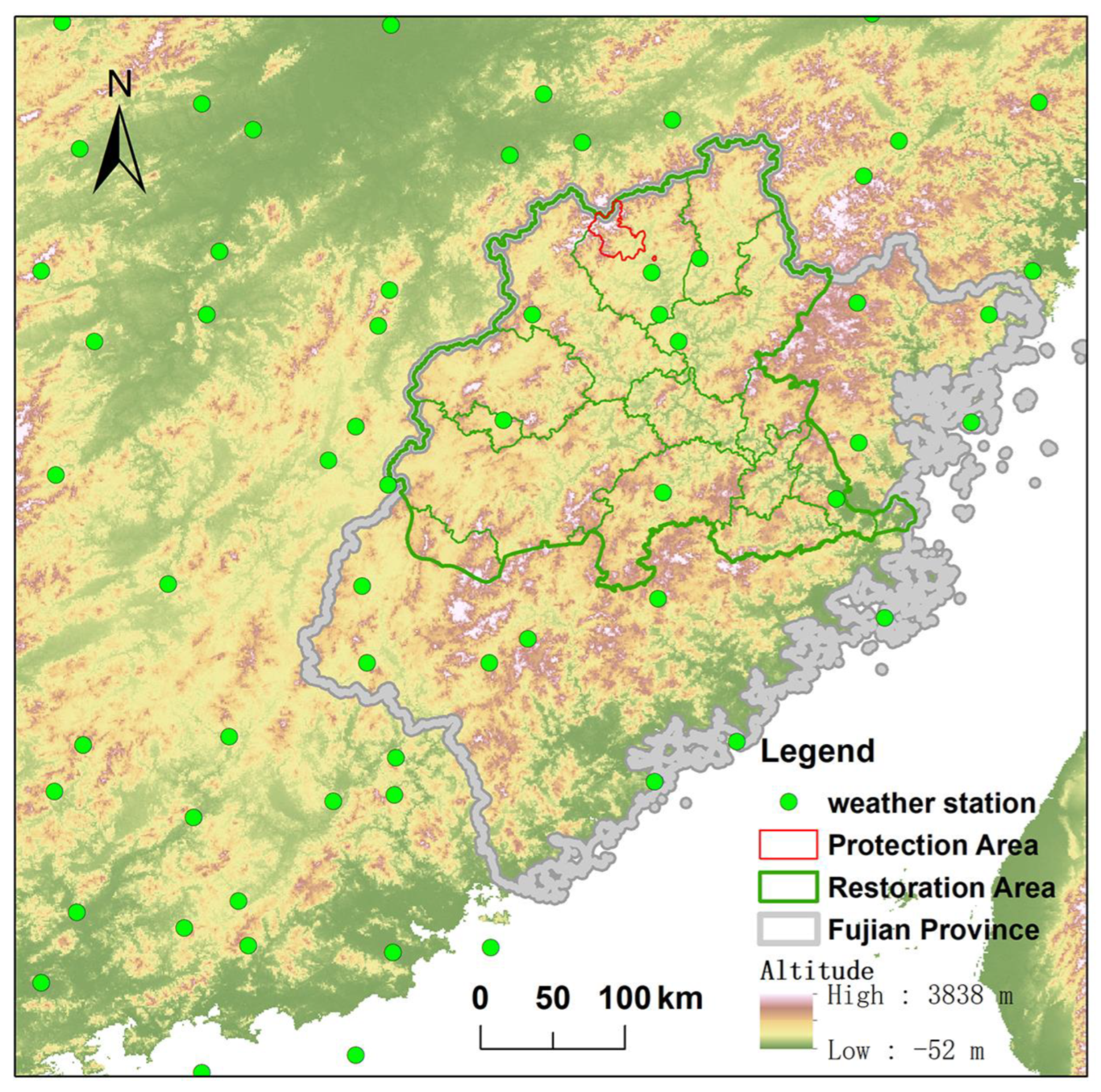
2.1. Description of the Study Area

The Fujian Province (terrestrial range between 115°50′–120°40′ E, 23°30′–28°22′ N) is in the hilly mountain belt of southeastern China (Figure 1), with an area of 12.4 × 10⁴ km2. The main soil types are red and yellow loam, and the soil layer is thin and barren. The main vegetation includes evergreen broad-leaved forests, evergreen coniferous forests, mixed coniferous forests, bamboo forests and so on.
The six leading industries are the electronic information and digital industry, the advanced equipment manufacturing industry, the petrochemical industry, the modern textiles and garments industry, the modern logistics industry, as well as tourism. Most industrial clusters are in coastal cities.
According to the Fujian Province Third Land Survey Main Data Bulletin (http://zrzyt.fujian.gov.cn (accessed on 1 December 2022)), the province’s cropland is in areas with annual precipitation of 800 mm or more. Among them, 84.8% are paddy fields; 3.4% are watered lands; and 11.8% are dry lands. The main food crop in the Fujian Province is rice, followed by soybeans, potatoes and so on. There are many kinds of vegetables and two main ways to grow them.
The vegetable greenhouses were mainly in the cities along the coast, and summer vegetable production areas with middle and high altitude were mainly in the middle part from the northeast to the southwest of Fujian.
There are several water systems, such as the Min River, the Jiulong River, the Jin River, the Jiaoxi River and the Ting River. Among them, the Minjiang watershed (116°23′–119°43′ E, 25°23′–28°19′ N) is crucial in the Fujian Province for ecological protection and restoration. The watershed occupies an area of 6.1 × 10⁴ km2. It has a subtropical monsoon climate with a warm and humid climate. The average annual temperature is approximately 18 °C, and the annual precipitation is approximately 1700 mm. The Shan-Shui Initiative in the Minjiang watershed includes five kinds of measures: water environment management and ecological restoration, biodiversity conservation, soil erosion management and ecological function enhancement of farmland, ecological restoration of abandoned mines and geological disaster prevention, as well as control, mechanism innovation and capacity building. There are 22 major projects located in 15 ecological restoration areas in this watershed (Table 1).
In the upper reaches of the Minjiang watershed, the Wuyi Mountains region is the largest mountainous area in the province and is rich in natural resources. It is one of the 11 key areas of global significance for biodiversity conservation in the country’s terrestrial areas. National nature reserves have been established in and around the Wuyi Mountains.
In this study, the range of the Shan-Shui Initiative in the Minjiang watershed was regarded as the restoration area, and the Wuyi Mountains national nature reserves and their surroundings were regarded as the protection area.

2.2. Data Sources

The land use types were obtained from the GlobeLand30 dataset, which is submitted by China to the UN (http://www.globeland30.com (accessed on 1 December 2022)). The land use types were divided into cropland, forest, grassland, shrubland, wetland, water body, artificial surface, bare land and others.
The range of the Shan-Shui Initiative in the Minjiang watershed was obtained from the Land Consolidation and Rehabilitation Center, Ministry of Nature Resources.
The annual precipitation was based on the climate data from the Data Center of China Meteorological Administration (https://data.cma.cn/ (accessed on 1 December 2022)). A total of 53 weather stations were selected to obtain the yearly precipitation data inside the Fujian Province and its surroundings (Figure 1). After excluding the data outliers, the elevation was introduced as a covariable to perform the interpolation with ANUSPLIN [48].
The grain, vegetable, meat and milk production and consumption data were from the Fujian Provincial Statistical Yearbook (https://tjj.fujian.gov.cn/xxgk/ndsj/ (accessed on 1 December 2022)).
The water consumption data were based on the Water Resources Bulletin of Fujian Province (http://slt.fujian.gov.cn/xxgk/tjxx/jbgb/ (accessed on 1 December 2022)).
The population density data were from the LandScan dataset which was published by the Oak Ridge National Laboratory of the United States Department of Energy (https://landscan.ornl.gov/ (accessed on 1 December 2022)) and was modified with China Census data from the China National Bureau of Statistics.
The nighttime lighting data were from the Prolonged Artificial Nighttime-light Dataset of China (1984–2020) which was provided by the National Tibetan Plateau Data Center (https://data.tpdc.ac.cn/zh-hans/data (accessed on 1 December 2022)) [49].
Carbon emission data were from the China County and District Carbon Emission Data (1997–2020), which were prepared according to the latest revision of energy data from the China National Bureau of Statistics (2015). Data of 2018–2020 were calculated by the interpolation method [50,51,52].
The soil and root properties were obtained from the Harmonized World Soil Database v1.2, which was released by the Food and Agriculture Paganization of the United Nations (https://www.fao.org/soils-portal/soil-survey/soil-maps-and-databases/harmonized-world-soil-database-v12/en/ (accessed on 1 December 2022)).
The NDVI, DEM and potential evaporative dispersion data were collected from the resource and environment data cloud platform of the Institute of Geographic Science and Natural Resources Research, Chinese Academy of Sciences (http://www.resdc.cn (accessed on 1 December 2022)). All the spatial data were resampled with a 1 km × 1 km spatial resolution fishnet in the ArcGIS 10.8.

2.3. Statistical Analysis

2.3.1. The Supply and Demand of Ecosystem Services

(1)
Food production (FP)
An existing study showed a significant linear relationship between crop and livestock production and NDVI [53]. Since the supply and demand of aquatic products in the study area were mainly derived from seafood, aquatic products were not considered in this study. Based on the spatial distribution data of land use types, the total production of grains and vegetables was assigned according to the ratio of grid NDVI values to the total NDVI values of cultivated land. Similarly, the production of meat and dairy was assigned according to the ratio of grid NDVI values to the total NDVI values of grassland. Then, the spatial distribution of the food supply was calculated by Equation (1):
F o o d s u = N D V I c r o p _ i N D V I c r o p _ s u m × G V s u m + N D V I g r a s s _ i N D V I g r a s s _ s u m × M D s u m
where Foodsu represents the food supply (t); NDVIcrop_i and NDVIgrass_i represent the NDVI value of grid i; NDVIcrop_sum and NDVIgrass_sum represent the total NDVI of cropland and grassland; GVsum represents the total production of grain and vegetables in the Fujian Province (t); and MDsum represents the total production of meat and milk in the Fujian Province (t).
Food demand was calculated by using per person food demand and population density, shown by Equation (2):
F o o d d e = F o o d p e r × P o p u l a t i o n i
where Foodde represents the food demand (t); Foodper represents the grain, vegetable, meat and milk demand per person (t); and Populationi represents the population density of grid i.
(2)
Water yield (WY)
The water supply was calculated by the “Water Yield” module of the InVEST model, which was based on the water balance method. The WY supply was obtained by subtracting actual evaporation from precipitation. The calculation was based on Budyko’s water-heat coupling theory and the average annual precipitation as in Equation (3) [54,55,56]:
E i = 1 A E T i P i · P i
where E(i) represents the annual WY supply of grid i (mm); AET(i) represents the annual actual evaporation of grid i (mm); and P(i) represents the annual precipitation of grid i (mm).
The AET(i) was calculated as Equation (4):
A E T i P i = 1 + P E T i P i 1 + P E T i P i w ( i ) 2 / w ( i )
where PET(i) represents the annual potential evaporation of grid i (mm); w(i) represents dimensionless parameters for climate and soil; and the meanings of other variables are the same as in Equation (3).
The w(i) was calculated in as Equation (5):
w ( i ) = Z · A W C i P i + 1.25
where Z represents seasonal index; AWC(i) represents the soil-available water content of grid i (mm); and the meanings of other variables are the same as in Equation (4).
The AWC(i) was calculated as in Equation (6):
A W C i = min ( M ax S o i l D e p t h i , R o o t D e p t h i ) P A W C i
where Max Soil Depth(i) represents maximum soil depth; RootDepth(i) represents the root depth; and PAWC(i) represents the plant-available water content of grid i (mm).
The water demand was divided into agricultural water, industrial water and other water. Agricultural water demand was assigned to the cropland grid according to NDVI weights. Industrial water demand was assigned to the artificial land grid according to the nighttime light intensity weight. Other water use was assigned to the grid according to the population density weight. The spatial distribution of water demand was calculated by Equation (7):
W a t e r d e = N D V I c r o p _ i N D V I c r o p _ s u m × W c r o p + N L a r t i _ i N L a r t i _ s u m × W a r t i + P D i P D s u m × W o t h e r s
where the Waterde represents the water demand (mm); NDVIcrop_i represents the NDVI value of grid i; NDVIcrop_sum represent the total NDVI of cropland and grassland; NLarti_i represents the nighttime light intensity of grid i; NLarti_sum represents the total nighttime light intensity of artificial surface; PDi represents the population density of grid i; PDsum represents the total population of the Fujian Province; and Wcrop, Warti and Wothers represent agricultural water, industrial water and other water (mm), respectively.
(3)
Soil retention (SR)
The SR was calculated by using the “SDR model” from the InVEST model based on the revised universal soil loss equation (RUSLE), considering the sediment transport ratio and deposition existing in the actual soil erosion process with Equation (8) [57,58,59,60]:
S M i = R K L S ( i ) U S L E ( i ) + S E D R ( i )
where the SM(i) represents the soil retention amount of grid i (t); RKLS(i) represents the potential soil erosion amount of grid i (t); USLE(i) represents the actual soil erosion amount of grid i (t); and SEDR(i) represents the retention of sediment intercepted by grid i itself (t).
The RKLS(i) were calculated as Equation (9):
R K L S i = R i · K i · L i · S i
where R(i) represents the rainfall erosivity factor of grid i (MJ mm/ha/hr); K(i) represents the soil erodibility factor of grid i (t ha hr/MJ/ha/mm); and L(i) and S(i) represent the slope and length factors, respectively.
The USLE(i) were calculated as Equation (10):
U S L E i = R K L S i · C i · P i
where C(i) and P(i) represent the vegetation cover crop management factor and soil and water conservation engineering measures factor for grid cell i (between 0–1), respectively; and the meanings of other variables are the same as in Equation (8).
The SEDR(i) were calculated as Equation (11):
S E D R i = S E i · j = 1 i 1 U L S E j · k = j + 1 i 1 · 1 S E k
where SE(i) represents the retention rate of grid i; USLE(j) represents the amount of sediment generated by the uphill grid j (t); and SE(k) represents the sediment retention by uphill grid (t)
Soil erosion, as an unwanted ecological activity, is the part of soil erosion that humans want to reduce. Therefore, the demand for SR was calculated as the actual erosion component of the soil by using the universal soil loss equation (USLE), as shown in Equation (9).
(4)
Carbon sequestration (CS)
Existing studies have shown that net primary productive (NPP) reflects the productivity of vegetation communities in the natural environment, and the carbon fixation capacity of the ground surface. It was equal to the carbon absorbed by plants through photosynthesis minus the carbon released by respiration. Soils in Fujian were very thin, and carbon fixation was mainly carried out by the above-ground parts of plants. Therefore, NPP was chosen to characterize the supply of regional CS services in this paper [61,62,63,64].
The CS demand was calculated by using the nighttime light intensity and the total carbon emissions. Existing studies have shown that there is a significant correlation between nighttime light brightness values and regional carbon emissions. This paper assumed that all carbon emissions from human activities need to be fixed in terrestrial ecosystems as CS demand, calculated by Equation (12):
C S d e = N L i N L s u m × C a r b o n s u m
where the CSde represents the CS demand (t); NLi represents the nighttime light intensity of grid cell i; NLsum represents the total nighttime light intensity of the Fujian Province; and Carbonsum represents the total carbon emissions of the Fujian Province.

2.3.2. The Trade-Offs/Synergies of Ecosystem Services

The correlation between vegetation coverage and variables was calculated by Pearson correlation analysis pixel-by-pixel. The correlation coefficient was calculated using Equation (13) [33,65]:
r x y = i = 1 n x i X ¯ y i Y ¯ i = 1 n x i X ¯ 2 i = 1 n y i Y ¯ 2
where n represents the number of samples, xi and yi represent the value of two kinds of ecosystem services at grid cell i, respectively; X ¯ and Y ¯ represent the mean value of the two kinds of ecosystem services, respectively; and rxy represents the correlation coefficient between the two kinds of ecosystem services. When this value is greater than zero, it indicates a synergistic relationship between the two ecosystem services. When the value is less than zero, there is a trade-off between the two ecosystem services.

2.3.3. The ESs Supply–Demand Relationships

The relationship between ESs supply and demand was analyzed by the supply–demand ratio. It could reflect the match between the supply and demand of ecosystem services. When the supply–demand ratio >0, it indicates that the supply is greater than the demand. When the supply–demand ratio <0, it indicates that the supply does not meet demand. The supply–demand ratio was calculated using Equation (14) [66,67,68]:
S D R i = S U i D E i S U m a x + D E m a x / 2
where the SUi and DEi represent the supply and demand of the same ecosystem service at the same time, respectively; and the SUmax and DEmax represents the maximum supply and demand of the same ecosystem service at the same time in the study area, respectively.

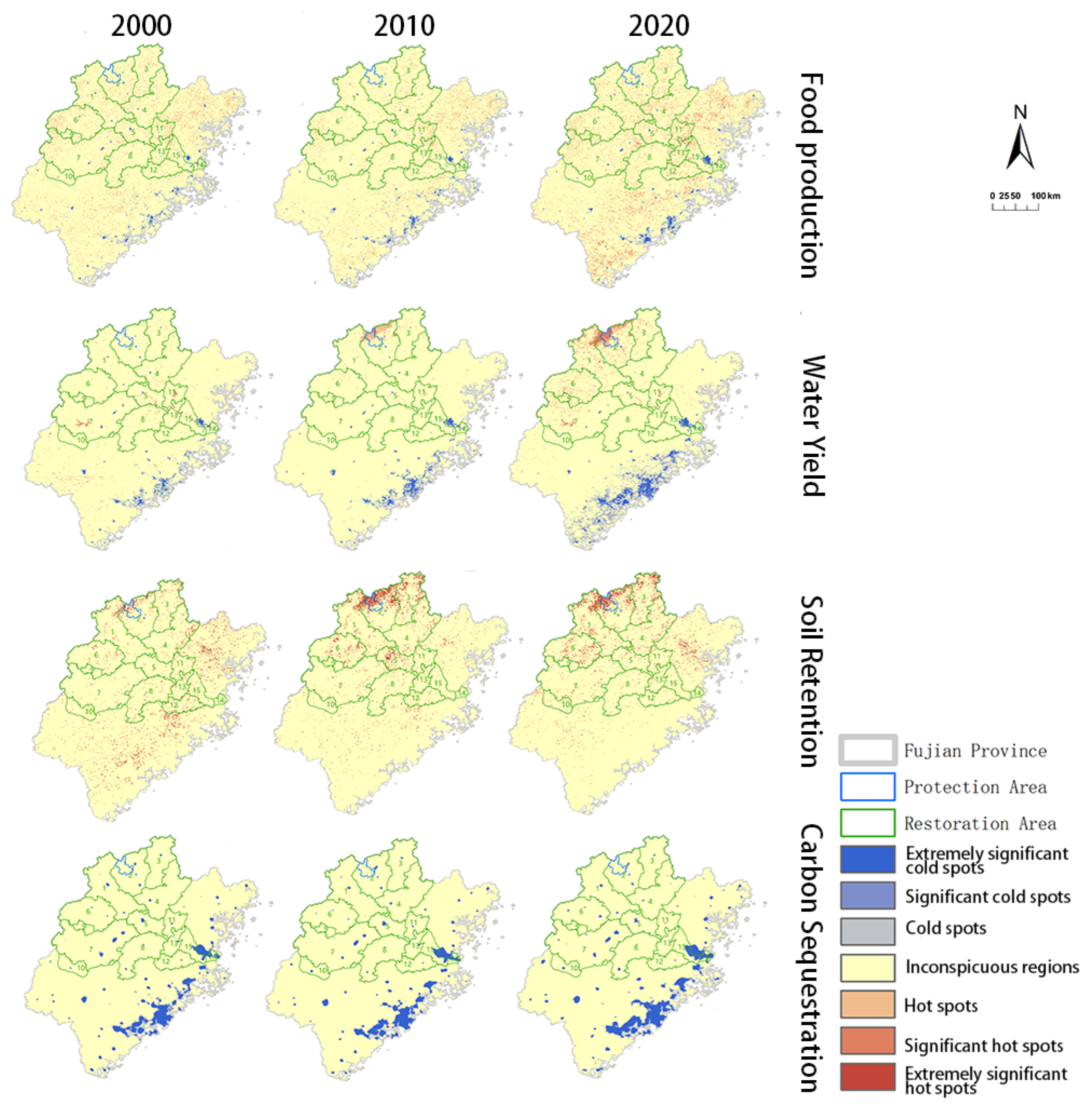
2.3.4. Spatial Clustering Analysis of the Supply–Demand Relationships

The Getis–Ord G i * index was used to analyze the hot and cold spots of supply–demand ratio to characterize their significant high and low values of clustering areas. The z-scores and p-values were measures of statistical significance which showed whether to reject the null hypothesis, feature by feature. A high z-score and small p-value for a feature indicates a spatial clustering of high values. The G i * index was calculated by Equation (15) [69,70,71]:
G i * = j n w i j x j j n x j
where the wij represents a symmetric one/zero spatial weight matrix with ones for all links defined as being within distance of a given i; and n represents the total number of patches.
The z-score was calculated by Equation (16) [69,70,71]:
Z G i * = j = 1 n w i j x j x ¯ j = 1 n w i j S D n j = 1 n w i j 2 j = 1 n w i j 2 n 1
where Z(Gi*) represents the z-score; x ¯ represents the average value of an ecosystem service; SD represents the standard deviation of an ecosystem service; and the meanings of other variables are the same as in Equation (15).
The hot/cold spots confidence levels were analyzed with Table 2.

3. Results

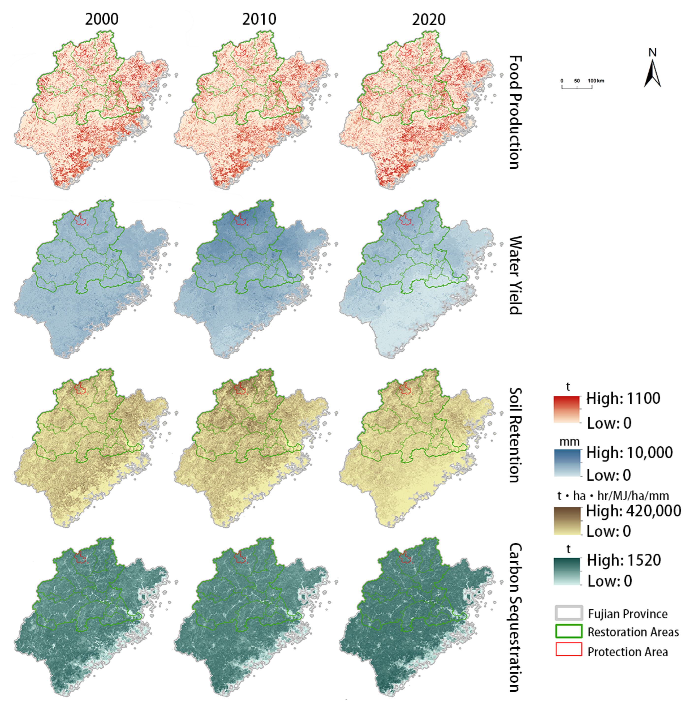
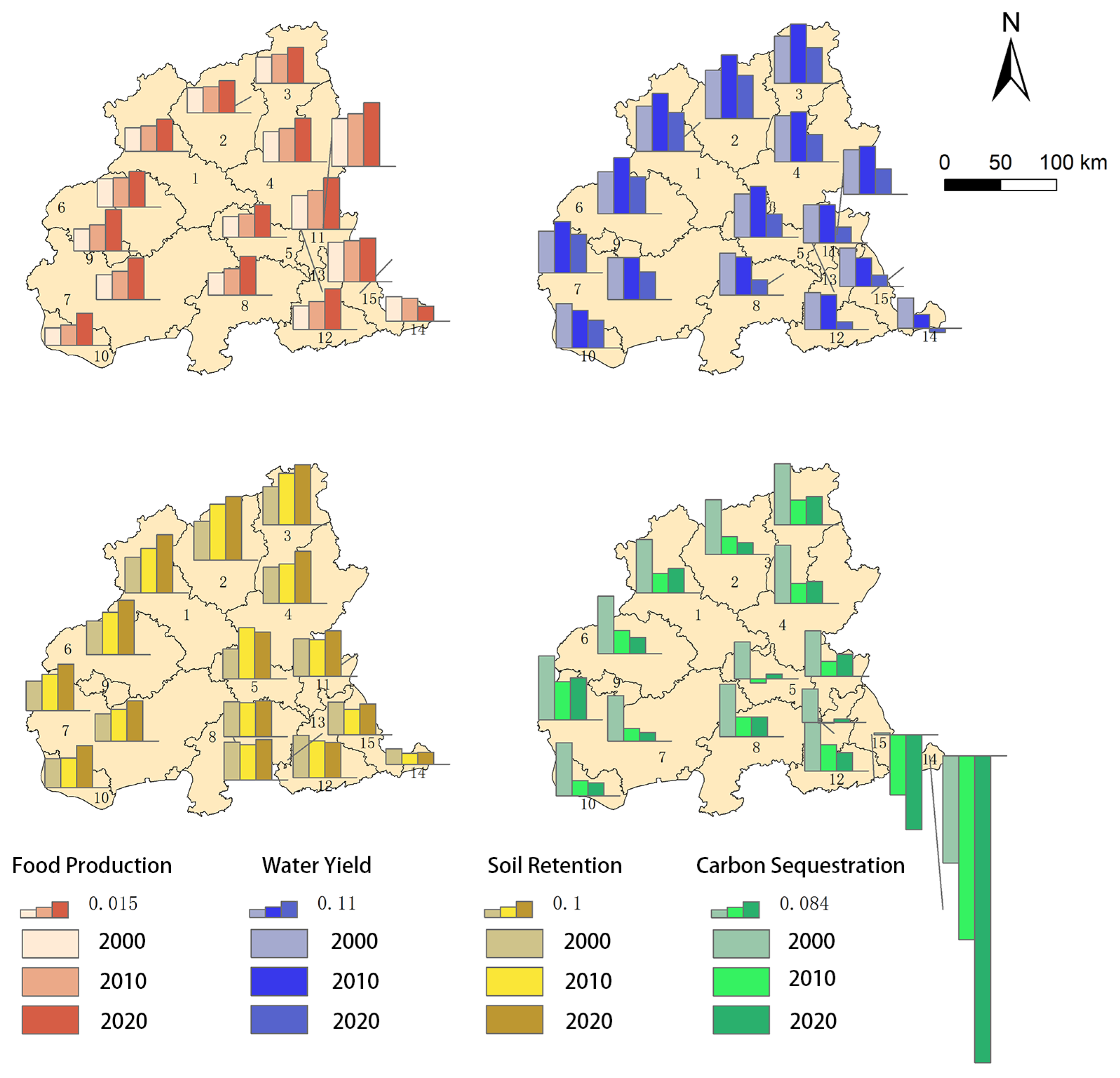
3.1. Variation in the ESs Supply and Their Relationships

The distribution of the ESs supply and temporal variation rates are shown in Figure 2 and Table 3. The mean value of the ESs supply and its rate of change varied significantly among regions. The supply of WY and SR was higher in the protected areas than in the restoration areas, and both were higher than that in other areas. FP showed the opposite pattern. CS was highest in the protected area in 2000 (926.79 t), while it changed to the restoration area in 2010 and 2020 with highest values of 922.68 t and 1014.91 t, respectively.
From 2000 to 2020, the supply of FP and CS increased, and WY and SR decreased in the Fujian Province (Table 3). The FP in each region decreased between 2000 and 2010 and increased between 2010 and 2020, with the largest changes in protected areas occurring during these two time periods. CS in the protection area decreased from 2000 to 2010 and increased in the other regions in both time periods. SR services showed an increasing and then decreasing trend in both protection and restoration areas, while they continued to decrease in other areas. The change rate was greatest in protected areas in these two time periods.
The variations in the relationships between different ESs are shown in Table 4. In the Fujian Province, the relationship between FP and WY and that between CS and SR showed synergistic relationships. There were trade-off relationships between FP and SR, between FP and CS and between WY and CS. The relationship between WY and SR changed from trade-off (−0.07) to synergy (0.37) from 2000 to 2020. The relationship between WY and CS in the protection area gradually changed from synergistic (0.23) to trade-off (0.03), while the restoration and other regions always showed trade-off relationships. The intensity of trade-offs or synergies between FP and other services was stronger in protection and restoration areas than in other areas.

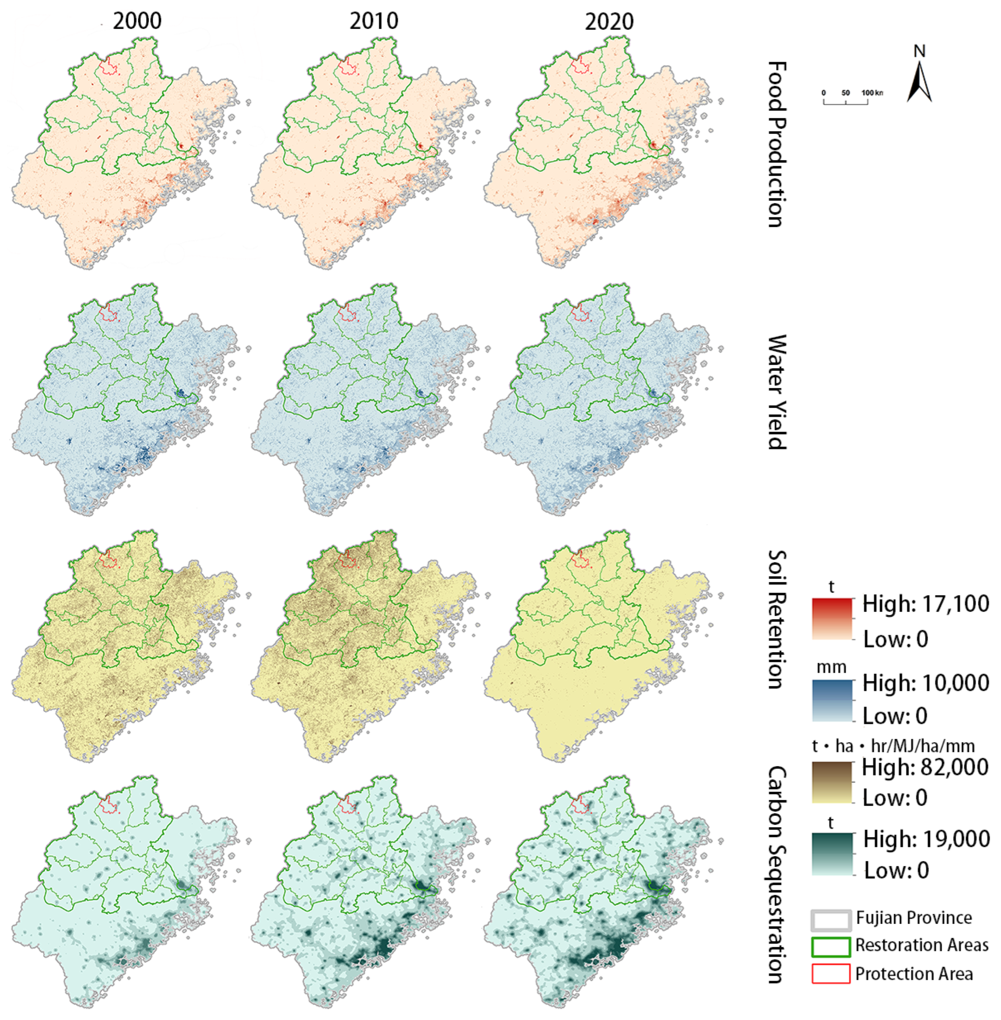
3.2. Variation in the ESs Demand

The distribution of the ESs supply and temporal variation rates are shown in Figure 3 and Table 5 and from 2000–2020, the demand for WY and CS increased, and the demand for FP and SR decreased in the Fujian Province (Table 5). WY demand decreased in protection areas and restoration areas from 2000–2020, where demand decreased from 2000–2010 and increased from 2010–2020, while other areas showed the opposite change. For CS demand, the value of protection areas decreased significantly between 2010 and 2020, while the difference was not significant in other areas and restoration areas.
. The mean value of ESs demand and its rate of change varied among regions. The demands for FP, WY and CS in the protection area were lower than those in the restoration area, and all were lower than those in other areas. The demand for SR showed an opposite variation pattern.
From 2000–2020, the demand for WY and CS increased, and the demand for FP and SR decreased in the Fujian Province (Table 5). WY demand decreased in protection areas and restoration areas from 2000–2020, where demand decreased from 2000–2010 and increased from 2010–2020, while other areas showed the opposite change. For CS demand, the value of protection areas decreased significantly between 2010 and 2020, while the difference was not significant in other areas and restoration areas.

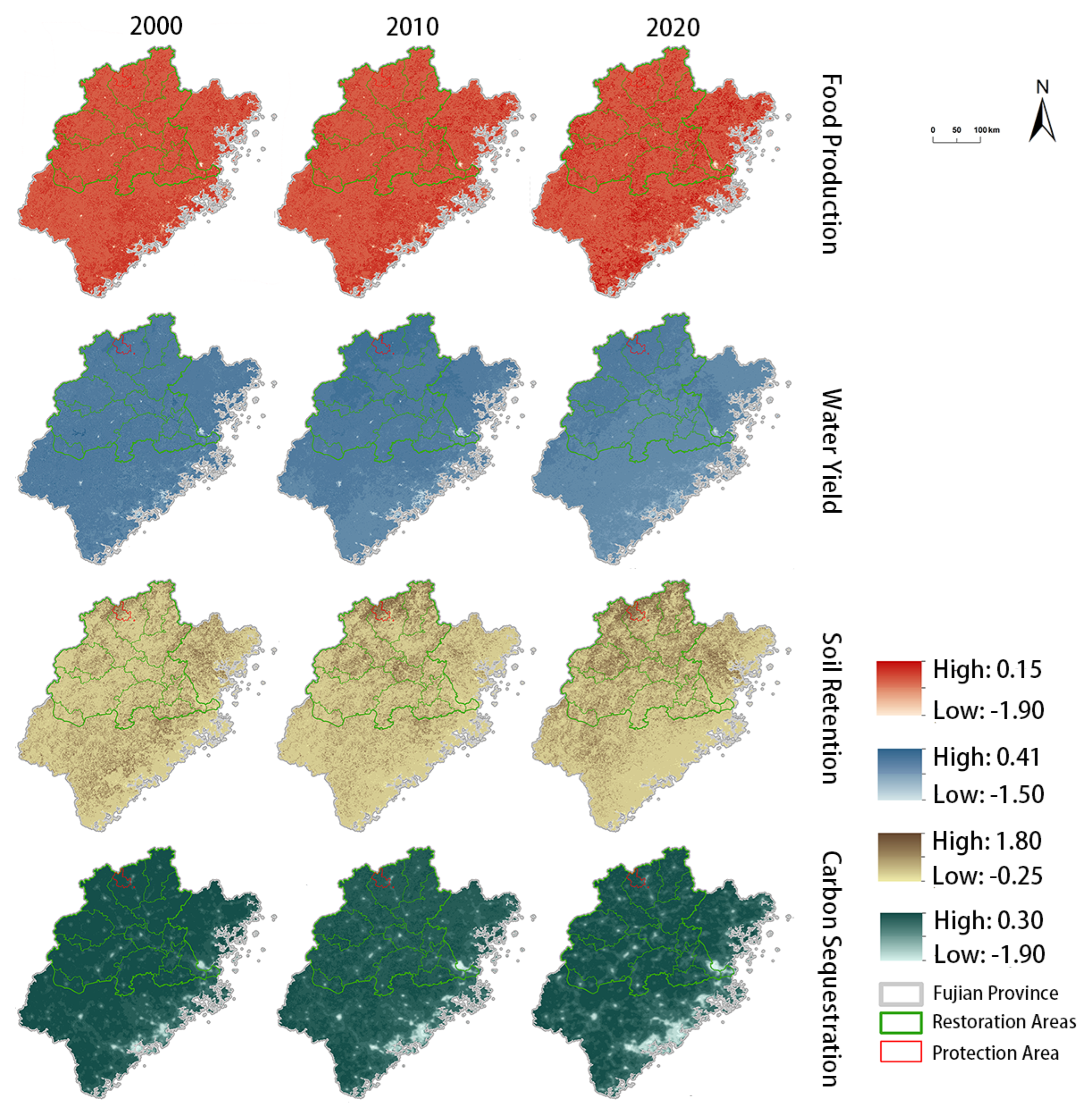
3.3. The Relationship between ESs Supply and Demand

Spatial and temporal variations in the ESs supply–demand ratio in different areas are shown in Figure 4 and Table 6. In all of the Fujian Province, ESs showed a trend of supply exceeding demand with strong spatial heterogeneity. The supply–demand ratio of FP increased in all areas during 2000–2020, while that of SR increased in protection and restoration areas and decreased in other areas. The supply–demand ratio of WY increased between 2000 and 2010 and decreased between 2010 and 2020 in protection and restoration areas. The supply–demand ratio of WY for other areas decreased from 2000 to 2020. For the CS, the supply changed from more than demand to less than demand in the other areas, and the imbalance between supply and demand increased, with the supply–demand ratio being 0.727, −0.0300 and −0.0612 in 2000, 2010 and 2020, respectively.
The spatial and temporal variations in the ESs supply-demand ratio in different subproject areas in the Minjiang Shan-Shui Initiative Project are shown in Figure 5. The supply-demand ratio of CS in each subproject area showed a decreasing trend during 2000–2010 and increased in some areas during 2010−2020, while that of WY showed the opposite pattern. For subproject area No. 14, the supply of CS and WY exceeds the demand. For subproject areas No. 5, 13 and 15, the supply of CS was lower than the demand in 2010, with CS still being undersupplied in subproject area No. 15 in 2020 (the supply-demand ratio is −0.2498). Although SR in subproject area No. 12 and FP services in subproject area No. 14 showed an excess of supply over demand, the supply-to-demand ratio continued to decrease over the period 2000−2020.
The hot and cold points of the ESs supply-demand ratio in 2020 are shown in Figure 6. In general, the cold spots of the supply-demand ratio for FP, WY and CS increased and that of SR decreased during 2000−2020 in the Fujian Province. The hot spots of the supply-demand ratio for WY and SR increased, while that of CS did not form a spatial cluster of high values. In the protection area, the high-value cluster areas for WY and SR gradually formed from 2000 to 2020. Most restoration areas have a high−value cluster of the supply–demand ratio for WY and SR. However, there were large areas of low-value clusters for the CS services supply-demand ratio in subproject areas No. 5, 7, 14 and 15. In addition, the cold spot clusters for the CS supply-demand ratio increased in subproject area No. 2, which was located around the protection area. The cold spots cluster of the supply-demand ratio for WY, CS and FP increased during the study period in subproject area No. 14, which was close to the provincial capital city.

4. Discussion

4.1. Changing Characteristics of Ecosystem Services under Ecosystem Protection and Restoration

Ecological protection and restoration are important ways to enhance ecosystem services and optimize the relationship between their supply and demand [39,45]. Ecological protection refers to the various preventive and control measures taken by people in various production and living dialogs to avoid or minimize the negative impact on the ecological environment. For ecological restoration, the goal in China was shifting from optimizing ecosystem structure and function to enhancing both human well-being and ecosystem quality [45]. It also started to focus on the effectiveness of ecosystem services and the balance between supply and demand [30,72,73]. The coastal hilly areas of southeast China have seen an increase in vegetation cover in recent years following a series of ecological protection and restoration efforts [38]. However, the study area entered a new stage of accelerated industrialization and urbanization, and the intensity of human activities such as mining increased, which increased the load on the local ecosystem [22]. In that case, changes and the balance of ecosystem services require further study.
Although some ESs showed synergistic relationships with each other, there were trade-offs between supporting and regulating services, particularly between CS and WY (Table 4). Existing ecological conservation and restoration measures have had limited effects in mitigating the intensity of trade-offs between different ESs in the Fujian Province. Our study also showed that the strength of trade-offs or synergies between FP and other ESs was stronger in protection and restoration areas than in other areas (Table 4). The supply of SR and WY was often strongly influenced by precipitation [74,75]. In general, they both decreased during the study period and showed a different pattern of change before and after 2010, except in the protection areas (From 2000 to 2020, the supply of FP and CS increased, and WY and SR decreased in the Fujian Province (Table 3). The FP in each region decreased between 2000 and 2010 and increased between 2010 and 2020, with the largest changes in protected areas occurring during these two time periods. CS in the protection area decreased from 2000 to 2010 and increased in the other regions in both time periods. SR services showed an increasing and then decreasing trend in both protection and restoration areas, while they continued to decrease in other areas. The change rate was greatest in protected areas in these two time periods.
CS continued to increase over the study period. In contrast to the other services, the value in protection areas showed the smallest increase and even a decline between 2000 and 2010 (From 2000 to 2020, the supply of FP and CS increased, and WY and SR decreased in the Fujian Province (Table 3). The FP in each region decreased between 2000 and 2010 and increased between 2010 and 2020, with the largest changes in protected areas occurring during these two time periods. CS in the protection area decreased from 2000 to 2010 and increased in the other regions in both time periods. SR services showed an increasing and then decreasing trend in both protection and restoration areas, while they continued to decrease in other areas. The change rate was greatest in protected areas in these two time periods.
The following reasons might explain the CS variation. First, the background value of CS in the protection area was high and there was little space for growth. Second, the newly planted grasses or trees after the implementation of the reforestation projects had not yet grown up, and the time point chosen for this study might also be subject to some coincidence. Third, some ecological restoration projects have reduced CS services, e.g., studies on farmland in the study area showed that land consolidation enhanced SR services, but reduced CS [36]. Fourth, the time of implementation of the Shan-Shui Initiative was relatively short, and some of the ecological benefits had not yet been realized.

4.2. ESs Supply and Demand Relationships and Their Possible Impact Factors

Different ecological protection and restoration measures caused variation in ecosystem structure and patterns. These changes affected not only the capacity of ecosystems to provide services, but also the relationship between supply and demand for ecosystem services [76,77]. The balance between the supply and demand of ESs is important for the sustainable construction of ecological projects and the sustainable use of natural capital [78]. Trade-offs between different ESs types and between ESs supply and demand exist due to the limitation of natural resources and differences in the demands of different stakeholders [79,80]. In general, ESs in the Fujian Province were oversupplied, but there was great spatial heterogeneity and no areas of high-value clusters of CS supply-demand ratios (Table 6, Figure 6). Supply and demand in protection and restoration areas were more balanced than in other areas (Figure 1). The ESs provision in the protection area exceeded the demand and gradually formed high−value clustering areas for WY and SR supply-demand ratios from 2000 to 2020 (Figure 6). The high−value cluster increased in most of the subproject areas. In other areas, the low-value clusters of FP, WY, and CS service supply-demand ratios increased. Thus, ecological protection and restoration measures had positive effects on optimizing the supply-demand balance of ESs, while some subproject areas needed to further improve the effectiveness of restoration.
Integrated with the existing studies, we explored the possible influencing factors. Regarding natural impact factors, precipitation, evapotranspiration and topography mainly affected the supply of WY and SR [29,81]. In this study, the protection area was in a mountainous area with complex topography and precipitation characteristics, and its supply and demand for SR were both higher than those of other areas (Figure 2 and Figure 3). Regarding human impact factors, land use has been recognized as one of the main factors affecting ESs [21,22,82]. In study areas with limited data, the use of land use type transfer matrices to analyze changes in supply and demand for ecosystem services has become an effective and feasible method. Another important impact factor is stakeholders’ preferences [82,83,84]. For example, changes in the diet structure of people affected the supply-demand ratio for FP. Although ESs are necessary for human well-being, the actual demand for and use of services by different stakeholder groups has been less considered in typical supply and demand analyses of ecosystem services [85]. Studies on coastal cities in the Fujian Province have shown that the supply capacity of ESs is spatially low offshore and high inland. The demand for ESs showed the opposite pattern, resulting in an imbalance between supply and demand in coastal areas. This was supported by Huang et al. [56], and similar patterns exist in the overall ESs supply and demand characteristics of the Fujian Province.
Many international studies have also supported the impact of land use change and stakeholder preferences on ESs. Studies on ecological protection areas have shown that drivers related to economic factors and land use change combine to create the different ecological problems faced inside and outside ecological protection areas [28]. There is a growing need to integrate ESs into protection area management strategies, and only a comprehensive ESs assessment can identify effective strategies for ecological protection and restoration. However, stakeholders are mostly ignored or only mentioned in ESs assessments related to protection areas [86]. In complex tropical forest frontier landscapes, researchers have found that land use and tenure and the demand for specific products are key determinants of final ES outcomes. While forests have a higher regulated and overall balanced ESs, mixed agricultural lands provide subsistence and commercial products, as well as better environmental education opportunities [73]. Research on river protection and management in the south−central United States suggests that it is both possible and useful to quantify the social demand for ecosystem services in watershed management, although the number of studies that use a sociocultural perspective in ecosystem service assessment is currently limited [80].

4.3. Implications for Ecosystem Protection and Restoration

The coastal hilly areas in southeastern of China have advanced economies and high population densities, and the ecosystem is greatly affected by human activities [46,47]. The ecological protection and restoration projects that have been carried out in the Fujian Province have resulted in higher vegetation coverage and reduced soil erosion and river pollution [87]. However, the spatial heterogeneity of regional ESs supply and demand relationships was strong, and imbalances between supply and demand still existed (Figure 4, Table 4). With climate change and increasingly intense human activity, ecosystem sustainability is under increasing threat [88,89,90]. The research on ESs provided references for scientifically and rationally implementing ecological protection and restoration as well as formulating development strategies that balance ecological and socioeconomic benefits. This study proposed some recommendations for further optimizing ecological protection and restoration strategies in the Fujian Province and other similar economically developed coastal provinces.
First, the layout of ecological protection and restoration projects and the selection of measures should focus on the spatial and temporal characteristics of ESs trade−offs and their supply-demand relationships. The implementation of existing ecological restoration projects was generally 5 years. However, ESs consist of complex biophysical processes and ecosystem networks, and the recovery of ecosystem services in ecological restoration projects might be delayed and incomplete [91]. Therefore, the imbalance between supply and demand and the trade−offs between different kinds of ESs in some restored areas (Table 4, Figure 5) might only be shown in the short term, and the long-term benefits in line with ecological principles need more attention. Ecological restoration projects that focus on specific ESs might negatively affect the supply of other services. A deeper understanding of how the supply of different ESs changed at different scales and identifying their sources of variation is an important direction for future research. This was also a key challenge for ecological restoration research [92]. Therefore, the development of ecological protection and restoration strategies requires a fair trade−off between primary and other objectives.
Second, the coastal areas and some of the restoration areas needed to focus on the potential needs of different stakeholders. ESs were often multigroup oriented, whereas not all stakeholders benefit from these services [93]. Identifying differences and interactions among different interest groups and reasonably assessing their diversity of perceptions, knowledge and preferences were necessary for a fair benefits distribution [77,94,95]. According to the IUCN Global Standard, a sustainable Nature-based Solution (NbS) should be economically viable and based on an equal empowerment governance process. In this study, the change in demand for each ecosystem service was analyzed based on multivariate data, and there were more areas of low-value clusters in the supply-demand ratio for ESs in coastal areas and some restoration areas (Figure 3 and Figure 6). The possible influences were multiple; for example, changes in food demand might be due to a combination of changes in population size and changes in diet structure. There might be a difference between stakeholders’ preferences and ecosystem service demands calculated from statistical data. Stakeholders’ preferences might influence the formulation of ecological restoration and economic development strategies, which may feedback to the financial flow and policies and institutional arrangements, and thus the sustainability of ecological restoration projects.
Third, ecological protection and restoration project design should focus on both intra- and extraterritorial effects and break the limits of administrative boundaries. To facilitate the implementation of ecological restoration projects, planning boundaries usually refer to administrative boundaries. However, ecosystems are a continuum, and a growing number of scholars and policymakers are realizing the importance of planning ecological restoration projects across administrative boundaries. According to our study, the distribution of high−value and low−value clusters of ESs supply and demand was across administrative boundaries (Figure 6). This had begun to be considered in the planning and implementation of the Shan-Shui Initiative, but the division of restoration units was still influenced by administrative boundaries. In addition, since the high− and low−value clusters of the ESs supply-demand ratio did not match spatially, ecological restoration projects should also consider extraterritorial effects at different scales. The development of comprehensive ecological restoration strategies, such as ecological compensation, requires a quantitative basis.
Fourth, ecological protection and restoration should focus on multiobjective optimization. Ecological protection and restoration in economically developed coastal areas should focus on the enhancement of CS services. The choice of ecological protection and restoration measures need to avoid negative impacts on other types due to a focus on a specific ecosystem service type. China proposed a goal that the nation achieves a carbon emission peak by 2030 and carbon neutrality by 2060. Ecological construction was also increasingly focused on this. According to our study, the area of the low−value cluster area of the CS service supply–demand ratio gradually increased in the coastal economically developed regions and some subproject areas, although the value of NPP increased (Figure 6). Although the supply of CS services in protection and restoration areas exceeded the demand, the supply-demand ratio continued to decline and needed to be considered.

4.4. Limitations of This Study

The ESs demand in this study was calculated based on data such as statistical yearbooks and has not yet considered the demand preferences of different stakeholders for different ESs. Future studies will obtain the preferences of different stakeholders for analysis through questionnaires and interviews. In addition, the socioeconomic impact of ecological protection and restoration should also be taken into consideration. On the other hand, since the implementation time of the Shan−Shui Initiative was relatively short for ecosystem succession, long-term monitoring was also needed. In the future, the impact of ecological protection and restoration projects on ESs could be analyzed with the impact of specific ecological restoration measures on ecosystem structure and function, thus providing more support for sustainable ecosystem development.

5. Conclusions

Taking the Fujian Province as an example, this paper analyzed the spatial patterns, temporal changes and supply-demand relationships of FP, WY, SR and CS supply and demand in ecological protection, restoration and other areas in 2000, 2010 and 2020. In general, the supply of ESs in the Fujian Province exceeded the demand, while the spatial distribution of supply and demand varied significantly. The ESs supply-demand ratio generally showed a decreasing trend from the mountainous regions in the northwest interior to the economically developed regions on the southeast coast. The ESs relationship between supply and demand in the protection areas was better than that in the restoration areas. The areas of the high−value WY cluster in and around the protection areas gradually increased. Other regions had larger areas of low−value clusters of the supply–demand ratio, especially WY and CS. Ecological restoration projects have improved the supply and demand for some ESs, but the supply-demand ratio for CS in some subproject areas needs to be a concern.
Under the influence of climate change and human activities, it was recommended to further strengthen the protection of mountainous areas in the northwestern region and carry out systematic ecological restoration in the economically developed coastal regions in the southeast. When selecting ecological restoration measures, attention should be given to the trade−offs and supply-demand relationships between different ESs. In addition, it was necessary to consider the internal and external effects of ecological restoration measures and to consider different stakeholders, so that ecological restoration projects were sustainable in both natural and human terms. This paper provides references for decision−making regarding scientific and reasonable ecological protection and restoration projects in hilly and mountainous regions and economically developed coastal regions.

Author Contributions

Data curation, X.Z., M.Z. and Y.G.; Formal analysis, X.Z.; Methodology, J.W.; Project administration, X.Z. & M.Z.; Supervision, J.W. & Y.L.; Writing—original draft, X.Z.; Writing—review & editing, J.W. & Y.L. All authors have read and agreed to the published version of the manuscript.

Funding

This research was financially supported by the National Natural Science Foundation of China (Project Grant No. 42001217) and the State Key Laboratory of Earth Surface Processes and Resource Ecology, Beijing Normal University (No. 2021-KF-11).

Data Availability Statement

The data that support the findings of this study are available from the corresponding author, upon reasonable request.

Conflicts of Interest

The authors declare no conflict of interest.

References

  1. Daily, G.C. Nature’s Services: Societal Dependence on Natural Ecosystems; Island Press: Washington, DC, USA, 1997. [Google Scholar]
  2. Fu, B.J. Ecosystem Service and Ecological Security; Higher Education Press: Beijing, China, 2013. [Google Scholar]
  3. Zhao, W.; Liu, Y.; Feng, Q.; Wang, Y.; Yang, S. Ecosystem services for coupled human and environment systems. Prog. Geogr. 2018, 37, 139–151, (Chinese with English abstract). [Google Scholar]
  4. Costanza, R.; de Groot, R.; Braat, L.; Kubiszewski, I.; Fioramonti, L.; Sutton, P.; Farber, S.; Grasso, M. Twenty years of ecosystem services: How far have we come and how far do we still need to go? Ecosyst. Serv. 2017, 28, 1–16. [Google Scholar] [CrossRef]
  5. Daily, G.C.; Matson, P.A. Ecosystem services: From theory to implementation. Proc. Natl. Acad. Sci. USA 2008, 105, 9455–9456. [Google Scholar] [CrossRef] [PubMed] [Green Version]
  6. Millennium Ecosystem Assessment. Ecosystems and Human Well-Being; Island Press: Washington, DC, USA, 2005. [Google Scholar]
  7. Costanza, R.; d’Arge, R.; Groot, R.d.; Farberk, S.; Grasso, M.; Hannon, B.; Limburg, K.; Naeem, S.; O’Neill, R.V.; Paruelo, J.; et al. The value of the world’s ecosystem services and natural capital. Ecol. Econ. 1998, 25, 3–15. [Google Scholar] [CrossRef]
  8. Costanza, R.; Fisher, B.; Mulder, K.; Liu, S.; Christopher, T. Biodiversity and ecosystem services: A multi-scale empirical study of the relationship between species richness and net primary production. Ecol. Econ. 2007, 61, 478–491. [Google Scholar] [CrossRef]
  9. Liu, X.; Zhao, W.; Liu, Y.; Hua, T.; Hu, X.; Cherubini, F. Contributions of ecological programs to sustainable development goals in Linzhi, over the Tibetan Plateau: A mental map perspective. Ecol. Eng. 2022, 176, 106532. [Google Scholar] [CrossRef]
  10. Lv, Y.; Fu, B.; Feng, X.; Zeng, Y.; Liu, Y.; Chang, R.; Sun, G.; Wu, B. A policy-driven large scale ecological restoration: Quantifying ecosystem services changes in the Loess Plateau of China. PLoS ONE 2012, 7, e31782. [Google Scholar] [CrossRef] [Green Version]
  11. Li, S.; Wang, Y.; Zhu, W.; Zhang, J.; Liu, Y.; Gao, Y.; Wang, Y.; Li, Y. Research framework of ecosystem services geography from spatial and regional perspectives. Acta Geogr. Sin. 2014, 69, 1628–1639. [Google Scholar]
  12. Fu, B.; Lv, Y.; Chen, L.; Su, C.; Yao, X.; Liu, Y. The latest progress of landscape ecology in the world. Acta Ecol. Sin. 2008, 28, 798–804. [Google Scholar]
  13. Su, C.; Fu, B. Discussion on links among landscape pattern, ecological precess, and ecosystem services. Chin. J. Nat. 2012, 34, 277–283. [Google Scholar]
  14. Naeem, W.; Xu, T.; Sutton, R.; Tiano, A. The design of a navigation, guidance, and control system for an unmanned surface vehicle for environmental monitoring. Proc. Inst. Mech. Eng. Part M J. Eng. Marit. Environ. 2008, 222, 67–79. [Google Scholar] [CrossRef] [Green Version]
  15. Kontogianni, A.; Luck, G.W.; Skourtos, M. Valuing ecosystem services on the basis of service-providing units: A potential approach to address the ‘endpoint problem’ and improve stated preference methods. Ecol. Econ. 2010, 69, 1479–1487. [Google Scholar] [CrossRef]
  16. Zander, K.K.; Straton, A. An economic assessment of the value of tropical river ecosystem services: Heterogeneous preferences among Aboriginal and non-Aboriginal Australians. Ecol. Econ. 2010, 69, 2417–2426. [Google Scholar] [CrossRef]
  17. Xie, G.; Zhang, C.; Zhang, C.; Xiao, Y.; Lu, C. The value of ecosystem services in China. Resour. Sci. 2015, 37, 1740–1746. [Google Scholar]
  18. Xie, G.; Zhang, C.; Zhen, L.; Zhang, L. Dynamic changes in the value of China’s ecosystem services. Ecosyst. Serv. 2017, 26, 146–154. [Google Scholar] [CrossRef]
  19. Schirpke, U.; Candiago, S.; Egarter Vigl, L.; Jager, H.; Labadini, A.; Marsoner, T.; Meisch, C.; Tasser, E.; Tappeiner, U. Integrating supply, flow and demand to enhance the understanding of interactions among multiple ecosystem services. Sci. Total Environ. 2019, 651, 928–941. [Google Scholar] [CrossRef]
  20. Shen, J.; Li, S.; Liang, Z.; Liu, L.; Li, D.; Wu, S. Exploring the heterogeneity and nonlinearity of trade-offs and synergies among ecosystem services bundles in the Beijing-Tianjin-Hebei urban agglomeration. Ecosyst. Serv. 2020, 43, 101103. [Google Scholar] [CrossRef]
  21. Shen, J.; Li, S.; Liu, L.; Liang, Z.; Wang, Y.; Wang, H.; Wu, S. Uncovering the relationships between ecosystem services and social-ecological drivers at different spatial scales in the Beijing-Tianjin-Hebei region. J. Clean. Prod. 2021, 290, 125193. [Google Scholar] [CrossRef]
  22. Shui, W.; Wu, K.; Du, Y.; Yang, H. The Trade-Offs between Supply and Demand Dynamics of Ecosystem Services in the Bay Areas of Metropolitan Regions: A Case Study in Quanzhou, China. Land 2021, 11, 22. [Google Scholar] [CrossRef]
  23. Karasov, O.; Heremans, S.; Kulvik, M.; Domnich, A.; Chervanyov, I. On How Crowdsourced Data and Landscape Organisation Metrics Can Facilitate the Mapping of Cultural Ecosystem Services: An Estonian Case Study. Land 2020, 9, 158. [Google Scholar] [CrossRef]
  24. Kubalikova, L. Cultural Ecosystem Services of Geodiversity: A Case Study from Stranska skala (Brno, Czech Republic). Land 2020, 9, 105. [Google Scholar] [CrossRef] [Green Version]
  25. Meng, Q.; Zhang, L.; Wei, H.; Cai, E.; Xue, D.; Liu, M. Linking Ecosystem Service Supply–Demand Risks and Regional Spatial Management in the Yihe River Basin, Central China. Land 2021, 10, 843. [Google Scholar] [CrossRef]
  26. Schröter, M.; Barton, D.N.; Remme, R.P.; Hein, L. Accounting for capacity and flow of ecosystem services: A conceptual model and a case study for Telemark, Norway. Ecol. Indic. 2014, 36, 539–551. [Google Scholar] [CrossRef]
  27. Serna-Chavez, H.M.; Schulp, C.J.E.; van Bodegom, P.M.; Bouten, W.; Verburg, P.H.; Davidson, M.D. A quantitative framework for assessing spatial flows of ecosystem services. Ecol. Indic. 2014, 39, 24–33. [Google Scholar] [CrossRef] [Green Version]
  28. Palomo, I.; Martín-López, B.; Potschin, M.; Haines-Young, R.; Montes, C. National Parks, buffer zones and surrounding lands: Mapping ecosystem service flows. Ecosyst. Serv. 2013, 4, 104–116. [Google Scholar] [CrossRef]
  29. Chen, D.; Li, J.; Yang, X.; Zhou, Z.; Pan, Y.; Li, M. Quantifying water provision service supply, demand and spatial flow for land use optimization: A case study in the YanHe watershed. Ecosyst. Serv. 2020, 43, 101117. [Google Scholar] [CrossRef]
  30. Castro, A.J.; Verburg, P.H.; Martín-López, B.; Garcia-Llorente, M.; Cabello, J.; Vaughn, C.C.; López, E. Ecosystem service trade-offs from supply to social demand: A landscape-scale spatial analysis. Landsc. Urban Plan. 2014, 132, 102–110. [Google Scholar] [CrossRef]
  31. Stürck, J.; Poortinga, A.; Verburg, P.H. Mapping ecosystem services: The supply and demand of flood regulation services in Europe. Ecol. Indic. 2014, 38, 198–211. [Google Scholar] [CrossRef]
  32. Nedkov, S.; Burkhard, B. Flood regulating ecosystem services—Mapping supply and demand, in the Etropole municipality, Bulgaria. Ecol. Indic. 2012, 21, 67–79. [Google Scholar] [CrossRef]
  33. Wang, C.; Zhao, M.; Xu, Y.; Zhao, Y.; Zhang, X. Ecosystem Service Synergies Promote Ecological Tea Gardens: A Case Study in Fuzhou, China. Remote Sens. 2023, 15, 540. [Google Scholar] [CrossRef]
  34. Feng, X.; Fu, B.; Lu, N.; Zeng, Y.; Wu, B. How ecological restoration alters ecosystem services: An analysis of carbon sequestration in China’s Loess Plateau. Sci. Rep. 2013, 3, 2846. [Google Scholar] [CrossRef] [PubMed] [Green Version]
  35. Cao, S. Impact of China’s Large-Scale Ecological Restoration Program on the Environment and Society in Arid and Semiarid Areas of China: Achievements, Problems, Synthesis, and Applications. Crit. Rev. Environ. Sci. Technol. 2011, 41, 317–335. [Google Scholar] [CrossRef]
  36. Zhong, L.; Wang, J.; Zhang, X.; Ying, L. Effects of agricultural land consolidation on ecosystem services: Trade-offs and synergies. J. Clean. Prod. 2020, 264, 121412. [Google Scholar] [CrossRef]
  37. Ouyang, Z.; Zheng, H.; Xiao, Y.; Polasky, S.; Liu, J.; Xu, W.; Wang, Q.; Zhang, L.; Xiao, Y.; Rao, E.; et al. Improvements in ecosystem services from investments in natural capital. Science 2016, 352, 1455–1459. [Google Scholar] [CrossRef]
  38. Zhong, L.; Wang, J.; Zhang, X.; Ying, L.; Zhu, C. Effects of agricultural land consolidation on soil conservation service in the Hilly Region of Southeast China—Implications for land management. Land Use Policy 2020, 95, 104637. [Google Scholar] [CrossRef]
  39. Wang, J.; Zhong, L. Application of ecosystem service theory for ecological pretection and restoration of mountain-river-forest-field-lake-grassland. Acta Ecol. Sin. 2019, 39, 8702–8708. [Google Scholar]
  40. Fu, B. Several Key Points in Territorial Ecological Restoration. Bull. Chin. Acad. Sci. 2021, 36, 64–69. [Google Scholar]
  41. Peng, J.; Lyu, D.; Dong, J.; Liu, Y.; Liu, Q.; Li, B. Processes coupling and spatial integration: Characterizing ecological restoration of territorial space in view of landscape ecology. J. Nat. Resour. 2020, 35, 3–13. [Google Scholar]
  42. Li, S.; Xie, A.; Lyu, C.; Guo, X. Research Progress and Prospect for Land Ecosystem Services. China Land Sci. 2018, 32, 82–89. [Google Scholar]
  43. Liu, S.; Dong, Y.; Sun, Y.; Shi, F. Priority area of mountains-rivers-forests-farmlands-lakes-grasslands based on the improvement of ecosystem services: A case study of Guizhou Province. Acta Ecol. Sin. 2019, 39, 8957–8965. [Google Scholar]
  44. Kong, L.; Zheng, H.; Ouyang, Z. Ecological protection and restoration of forest, wetland, grassland and cropland based on the perspective of ecosystem services: A case study in Dongting Lake Watershed. Acta Ecol. Sin. 2019, 39, 8903–8910. [Google Scholar]
  45. Wang, J.; Ying, L.; Zhong, L. Thinking for the transformation of land consolidation and ecological restoration in the new era. J. Nat. Resour. 2020, 35, 26–36. [Google Scholar] [CrossRef]
  46. Ying, L.; Wang, J.; Zhou, Y. Ecological-environmental problems and solutions in the Minjiang River basin, Fujian Province, China. Acta Ecol. Sin. 2019, 39, 8857–8866. [Google Scholar]
  47. Ying, L.; Dong, Z.; Wang, J.; Mei, Y.; Shen, Z.; Zhang, Y. Rural economic benefits of land consolidation in mountainous and hilly areas of southeast China: Implications for rural development. J. Rural Stud. 2020, 74, 142–159. [Google Scholar] [CrossRef]
  48. Hutchinson, M.F.; Xu, T. Anusplin Version 4.4 User Guide; The Australian National University: Canberra, Australia, 2013; Available online: http://fennerschool.anu.edu.au/files/anusplin44.pdf (accessed on 1 December 2022).
  49. Zhang, L.; Ren, Z.; Chen, B.; Gong, P.; Fu, H.; Xu, B. A Prolonged Artificial Nighttime-Light Dataset of China (1984–2020); National Tibetan Plateau Data Center: Beijing, China, 2021. [Google Scholar]
  50. Shan, Y.; Liu, J.; Liu, Z.; Xu, X.; Shao, S.; Wang, P.; Guan, D. New provincial CO2 emission inventories in China based on apparent energy consumption data and updated emission factors. Appl. Energy 2016, 184, 742–750. [Google Scholar] [CrossRef] [Green Version]
  51. Shan, Y.; Guan, D.; Zheng, H.; Ou, J.; Li, Y.; Meng, J.; Mi, Z.; Liu, Z.; Zhang, Q. China CO2 emission accounts 1997–2015. Sci. Data 2018, 5, 170201. [Google Scholar] [CrossRef] [Green Version]
  52. Shan, Y.; Huang, Q.; Guan, D.; Hubacek, K. China CO2 emission accounts 2016–2017. Sci. Data 2020, 7, 54. [Google Scholar] [CrossRef] [Green Version]
  53. Peng, J.; Tian, L.; Liu, Y.; Zhao, M.; Hu, Y.; Wu, J. Ecosystem services response to urbanization in metropolitan areas: Thresholds identification. Sci. Total Environ. 2017, 607–608, 706–714. [Google Scholar] [CrossRef]
  54. Budyko, M.I. Climate and Life; Academic Press: San Diego, CA, USA, 1974. [Google Scholar]
  55. Feng, X.M.; Sun, G.; Fu, B.J.; Su, C.H.; Liu, Y.; Lamparski, H. Regional effects of vegetation restoration on water yield across the Loess Plateau, China. Hydrol. Earth Syst. Sci. 2012, 16, 2617–2628. [Google Scholar] [CrossRef] [Green Version]
  56. Zhang, B.; Li, W.; Xie, G.; Xiao, Y. Water conservation function and its measurement methods of forest ecosystem. Chin. J. Ecol. 2009, 28, 529–534. [Google Scholar]
  57. McCool, D.K.; Brown, L.C.; Foster, G.R.; Mutchler, C.K.; Meyer, L.D. Revised Slope Steepness Factor for the Universal Soil Loss Equation. Trans. ASAE 1987, 30, 1387–1396. [Google Scholar] [CrossRef]
  58. Williams, J.R.; Arnold, J.G. A system of erosion-sediment yield models. Soil Technol. 1997, 11, 43–55. [Google Scholar] [CrossRef]
  59. Wischmeier, W.H.; Smith, D.D. Rainfall energy and its relationship to soil loss. Trans. Am. Geophys. Union 1958, 39, 285–291. [Google Scholar] [CrossRef]
  60. Zhang, L.; Fu, B.; Lü, Y.; Zeng, Y. Balancing multiple ecosystem services in conservation priority setting. Landsc. Ecol. 2014, 30, 535–546. [Google Scholar] [CrossRef]
  61. Zhu, W.; Pan, Y.; Zhang, J. Estimation of net primary productivity of Chinese terrestrial vegetation based on remote sensing. J. Plant Ecol. 2007, 31, 413–424. [Google Scholar]
  62. He, Y.; Dong, W.; Ji, J.; Dan, L. The net primary production simulation of terrestral ecosystems in China by AVIM. Adv. Earth Sci. 2005, 20, 345–349. [Google Scholar]
  63. Potter, C.S.; Randerson, J.T.; Field, C.B.; Matson, P.A.; Vitousek, P.M.; Mooney, H.A.; Klooster, S.A. Terrestrial ecosystem production A process model based on global. Glob. Biogeochem. Cycles 1993, 7, 811–841. [Google Scholar] [CrossRef]
  64. Jia, X.; Fu, B.; Feng, X.; Hou, G.; Liu, Y.; Wang, X. The tradeoff and synergy between ecosystem services in the Grain-for-Green areas in Northern Shaanxi, China. Ecol. Indic. 2014, 43, 103–113. [Google Scholar] [CrossRef]
  65. Benesty, J.; Chen, J.; Huang, Y.; Cohen, I. Pearson correlation coefficient. In Noise Reduction in Speech Processing; Springer: Berlin/Heidelberg, Germany, 2009; pp. 1–4. [Google Scholar]
  66. Li, J.; Jiang, H.; Bai, Y.; Alatalo, J.M.; Li, X.; Jiang, H.; Liu, G.; Xu, J. Indicators for spatial–temporal comparisons of ecosystem service status between regions: A case study of the Taihu River Basin, China. Ecol. Indic. 2016, 60, 1008–1016. [Google Scholar] [CrossRef]
  67. Chen, J.; Jiang, B.; Bai, Y.; Xu, X.; Alatalo, J.M. Quantifying ecosystem services supply and demand shortfalls and mismatches for management optimisation. Sci. Total Environ. 2019, 650, 1426–1439. [Google Scholar] [CrossRef]
  68. Zhang, P.; Liu, S.; Zhou, Z.; Liu, C.; Xu, L. Supply and demand measurement and spatio-temporal evolution of ecosystem services in BeijingTianjin-Hebei Region. Acta Ecol. Sin. 2021, 41, 3354–3367. [Google Scholar]
  69. Getis, A.; Ord, J.K. The Analysis of Spatial Association by Use of Distance Statistics. Geogr. Anal. 2010, 24, 189–206. [Google Scholar] [CrossRef]
  70. Mashinini, D.P.; Fogarty, K.J.; Potter, R.C.; Berles, J.D. Geographic hot spot analysis of vaccine exemption clustering patterns in Michigan from 2008 to 2017. Vaccine 2020, 38, 8116–8120. [Google Scholar] [CrossRef] [PubMed]
  71. Scott, L.M.; Janikas, M.V. Spatial Statistics in ArcGIS. In Handbook of Applied Spatial Analysis; Fischer, M.M., Getis, A., Eds.; Springer: Heidelberg, Germany, 2009; pp. 27–41. [Google Scholar]
  72. King, E.; Cavender-Bares, J.; Balvanera, P.; Mwampamba, T.H.; Polasky, S. Trade-offs in ecosystem services and varying stakeholder preferences: Evaluating conflicts, obstacles, and opportunities. Ecol. Soc. 2015, 20, 25. [Google Scholar] [CrossRef] [Green Version]
  73. Feurer, M.; Zaehringer, J.G.; Heinimann, A.; Naing, S.M.; Blaser, J.; Celio, E. Quantifying local ecosystem service outcomes by modelling their supply, demand and flow in Myanmar’s forest frontier landscape. J. Land Use Sci. 2021, 16, 55–93. [Google Scholar] [CrossRef]
  74. Luo, R.; Yang, S.; Wang, Z.; Zhang, T.; Gao, P. Impact and trade off analysis of land use change on spatial pattern of ecosystem services in Chishui River Basin. Environ. Sci. Pollut. Res. 2021, 29, 20234–20248. [Google Scholar] [CrossRef]
  75. Li, J. Identification of ecosystem services supply and demand and driving factors in Taihu Lake Basin. Environ. Sci. Pollut. Res. 2022, 29, 29735–29745. [Google Scholar] [CrossRef]
  76. Bagstad, K.J.; Semmens, D.J.; Waage, S.; Winthrop, R. A comparative assessment of decision-support tools for ecosystem services quantification and valuation. Ecosyst. Serv. 2013, 5, 27–39. [Google Scholar] [CrossRef]
  77. Felipe-Lucia, M.R.; Martin-Lopez, B.; Lavorel, S.; Berraquero-Diaz, L.; Escalera-Reyes, J.; Comin, F.A. Ecosystem Services Flows: Why Stakeholders’ Power Relationships Matter. PLoS ONE 2015, 10, e0132232. [Google Scholar] [CrossRef] [Green Version]
  78. Shen, J.; Li, S.; Liang, Z.; Wang, Y.; Fuyue, S. Research progress and prospect for the relationships between ecosystem services supplies and demands. J. Nat. Resour. 2021, 36, 1909–1922. [Google Scholar] [CrossRef]
  79. Paavola, J.; Hubacek, K. Ecosystem Services, Governance, and Stakeholder Participation: An Introduction. Ecol. Soc. 2013, 18, 42. [Google Scholar] [CrossRef] [Green Version]
  80. Castro, A.J.; Vaughn, C.C.; Julian, J.P.; García-Llorente, M. Social Demand for Ecosystem Services and Implications for Watershed Management. JAWRA J. Am. Water Resour. Assoc. 2016, 52, 209–221. [Google Scholar] [CrossRef]
  81. Mitchell, M.G.E.; Bennett, E.M.; Gonzalez, A. Strong and nonlinear effects of fragmentation on ecosystem service provision at multiple scales. Environ. Res. Lett. 2015, 10, 094014. [Google Scholar] [CrossRef]
  82. Verburg, P.H.; Crossman, N.; Ellis, E.C.; Heinimann, A.; Hostert, P.; Mertz, O.; Nagendra, H.; Sikor, T.; Erb, K.-H.; Golubiewski, N.; et al. Land system science and sustainable development of the earth system: A global land project perspective. Anthropocene 2015, 12, 29–41. [Google Scholar] [CrossRef] [Green Version]
  83. Orenstein, D.E.; Groner, E. In the eye of the stakeholder: Changes in perceptions of ecosystem services across an international border. Ecosyst. Serv. 2014, 8, 185–196. [Google Scholar] [CrossRef]
  84. Chin, A.; Simon, G.L.; Anthamatten, P.; Kelsey, K.C.; Crawford, B.R.; Weaver, A.J. Pandemics and the future of human-landscape interactions. Anthropocene 2020, 31, 100256. [Google Scholar] [CrossRef]
  85. Darvill, R.; Lindo, Z. The inclusion of stakeholders and cultural ecosystem services in land management trade-off decisions using an ecosystem services approach. Landsc. Ecol. 2016, 31, 533–545. [Google Scholar] [CrossRef]
  86. Schirpke, U.; Scolozzi, R.; De Marco, C.; Tappeiner, U. Mapping beneficiaries of ecosystem services flows from Natura 2000 sites. Ecosyst. Serv. 2014, 9, 170–179. [Google Scholar] [CrossRef]
  87. Chen, C.; Park, T.; Wang, X.; Piao, S.; Xu, B.; Chaturvedi, R.K.; Fuchs, R.; Brovkin, V.; Ciais, P.; Fensholt, R.; et al. China and India lead in greening of the world through land-use management. Nat. Sustain. 2019, 2, 122–129. [Google Scholar] [CrossRef]
  88. Seddon, A.W.; Macias-Fauria, M.; Long, P.R.; Benz, D.; Willis, K.J. Sensitivity of global terrestrial ecosystems to climate variability. Nature 2016, 531, 229–232. [Google Scholar] [CrossRef] [Green Version]
  89. Stovall, A.E.L.; Shugart, H.; Yang, X. Tree height explains mortality risk during an intense drought. Nat. Commun. 2019, 10, 4385. [Google Scholar] [CrossRef] [PubMed] [Green Version]
  90. Smith, B.D.; Zeder, M.A. The onset of the Anthropocene. Anthropocene 2013, 4, 8–13. [Google Scholar] [CrossRef]
  91. Palmer, M.A.; Filoso, S. Restoration of ecosystem services for environmental markets. Science 2009, 325, 575–577. [Google Scholar] [CrossRef] [Green Version]
  92. Bullock, J.M.; Aronson, J.; Newton, A.C.; Pywell, R.F.; Rey-Benayas, J.M. Restoration of ecosystem services and biodiversity: Conflicts and opportunities. Trends Ecol. Evol. 2011, 26, 541–549. [Google Scholar] [CrossRef] [PubMed]
  93. Raum, S. A framework for integrating systematic stakeholder analysis in ecosystem services research: Stakeholder mapping for forest ecosystem services in the UK. Ecosyst. Serv. 2018, 29, 170–184. [Google Scholar] [CrossRef]
  94. Hauck, J.; Görg, C.; Varjopuro, R.; Ratamäki, O.; Jax, K. Benefits and limitations of the ecosystem services concept in environmental policy and decision making: Some stakeholder perspectives. Environ. Sci. Policy 2013, 25, 13–21. [Google Scholar] [CrossRef]
  95. Grima, N.; Fisher, B.; Ricketts, T.H.; Sonter, L.J. Who benefits from ecosystem services? Analysing recreational moose hunting in Vermont, USA. Oryx 2019, 53, 707–715. [Google Scholar] [CrossRef]
Figure 1. The site of the research area.
Land 12 00750 g001
Figure 2. Variation in the ecosystem services supply in the Fujian Province.
Land 12 00750 g002
Figure 3. Variation in the ecosystem services demand in the Fujian Province.
Land 12 00750 g003
Figure 4. Variation in the ecosystem services supply-demand ratio.
Land 12 00750 g004
Figure 5. Variations in the ESs supply-demand ratio in different subproject areas.
Land 12 00750 g005
Figure 6. The variation in hot and cold spots of the ecosystem services supply-demand ratio.
Land 12 00750 g006
Table 1. The 15 Main Sub-projects in Minjiang Shan-Shui Initiative.
NO.Main Sub-Project in Minjiang Shan-Shui Initiative
1Ecological Protection and Restoration Project at Futun Watershed and Abandoned Mine Comprehensive Improvement Project at Shunchang County
2Water Environment Management and Regional Ecological Protection and Restoration Project at Chongyang sub-watershed and River Comprehensive Improvement and Regional Ecological Protection and Restoration Project at Nanpu watershed
3Comprehensive Remediation of Abandoned Mines and Heavy Metal Contaminated Land Restoration Project at Pucheng County
4Water Environment Management and Regional Biodiversity Protection Project at Songxi and Jianxi sub-watershed and the surrounding area
6Ecological Protection and Restoration Project at Jinxi sub-watershed
5Water Environment Management and Regional Ecological Protection and Restoration Project at Yanping Section of Minjiang River and Ecological Monitoring and Management Capacity Building Project at Nanping City
8Ecological Protection and Restoration Project at Youxi sub-watershed
9International Migratory Bird Migration Corridor Protection and Restoration Project in the Mingxi Section of the Shaxi sub-watershed
7Ecological Protection and Restoration Project at Shaxi sub-watershed; Abandoned mine environment restoration and geological disaster prevention and control project; and Ecological Monitoring and Management Capacity Building Project at Sanming city
10Water Source Protection and Regional Ecological Protection and Restoration Project at upstream of Shaxi sub-watershed
11Water Environment Management and Regional Ecological Protection and Restoration Project at Gutianxi sub-watershed
12Water Environment Management and Regional Ecological Protection and Restoration Project Dazhangxi sub-watershed
13Water Environment Management and Regional Ecological Protection and Restoration Project Meixi sub-watershed
14Water Environment Management and Wetland Protection Project at Changle section of Minjiang river
15Water Environment Management and Wetland Protection Project at Houle section of Minjiang river
Table 2. The hot/cold spots confidence level.
Hot/Cold Spot Levelz-Scorep-Value
Extremely significant hot spots>2.58<0.01
Significant hot spots1.96–2.58<0.05
Hot spots1.65–1.96<0.10
Inconspicuous regions−1.65–1.65-
Cold spots−1.96–1.65<0.10
Significant cold spots−2.58–1.96<0.05
Extremely significant cold spots<2.58<0.01
Table 3. The ecosystem services supply mean values in different areas and their variation rate.
Area200020102020VR2000-2010 (%)VR2010-2020VR2000-2020
FP supply (t)
Total178.18169.81186.52−4.70%9.84%4.47%
OM206.01195.23206.80−5.23%5.93%0.38%
MJ146.97141.30163.76−3.86%15.90%10.25%
WYS94.1683.28100.83−11.56%21.08%6.62%
WY supply (mm)
Total778.41830.33329.0725.76%−51.89%−65.27%
OM784.67986.79474.796.67%−60.37%−136.55%
MJ791.701162.27638.2446.81%−45.09%−24.04%
WYS923.801663.201024.4780.04%−38.40%9.83%
CS supply (t)
Total877.27896.58995.342.20%11.02%11.86%
OM849.97873.31977.902.75%11.98%13.08%
MJ907.89922.681014.911.63%9.99%10.54%
WYS926.79903.84954.89−2.48%5.65%2.94%
SR supply (t·ha·hr/MJ/ha/mm)
Total24,332.4227,565.2617,763.1313.29%−35.56%−36.98%
OM23,988.0021,808.9913,599.52−9.08%−37.64%−76.39%
MJ24,716.9733,992.2922,411.7537.53%−34.07%−10.29%
WYS39,871.9669,773.5641,362.8574.99%−40.72%3.60%
Note: Total represents the whole Fujian area; OM represents areas outside the Minjiang Shan-Shui Initiative Project (the other areas); MJ represents the Minjiang Shan-Shui Initiative Project areas (the restoration area); WYS represents the Wuyi mountain national nature reserves and their surroundings (the protection area); and VR represents the variation rate.
Table 4. Variations in the relationships between different ESs supplies.
YearFP & WYFP & SRFP & CSWY & SRWY & CSWCS & SR
Total20000.31 **−0.16 **−0.18 **−0.07 **−0.24 **0.42 **
20100.08 **−0.17 **−0.13 **0.35 **−0.04 **0.36 **
20200.05 **−0.15 **−0.06 **0.37 **−0.05 **0.30 **
OM20000.27 **−0.16 **−0.17 **−0.13 **−0.31 **0.45 **
20100.11 **−0.15 **−0.11 **0.15 **−0.13 **0.44 **
20200.01−0.13 **−0.05 **0.29 **−0.07 **0.38 **
MJ20000.37 **−0.17 **−0.19 **0.01 *−0.11 **0.37 **
20100.20 **−0.17 **−0.17 **0.31 **−0.06 **0.31 **
20200.22 **−0.15 **−0.08 **0.21 **−0.15 **0.24 **
WYS20000.21 **−0.23 **−0.35 **0.33 **0.23 **0.47 **
20100.18 **−0.20 **−0.25 **0.40 **0.08 *0.328 **
20200.19 **−0.22 **−0.12 **0.29 **−0.030.13 **
Notes: ** Significant correlation at the 0.01 level (2-tailed); * Significant correlation at the 0.05 level (2-tailed); Total represents the whole Fujian area; OM represents areas outside the Minjiang Shan-Shui Initiative Project (the other areas); MJ represents the Minjiang Shan-Shui Initiative Project areas (the restoration area); WYS represents the Wuyi mountain national nature reserves and their surroundings (the protection area); FP, WY, SR and CS represent the food production, water yield, soil retention and carbon sequestration supply, respectively; a positive value indicates a synergistic relationship, while a negative value indicates a trade-off relationship.
Table 5. The ecosystem services’ demand mean values in different areas and their variation rate.
Location200020102020VR2000-2010VR2010-2020VR2000-2020
FP demand (t)
Total72.4262.7265.00−13.39%3.64%−11.40%
OM103.2792.4999.05−10.44%7.09%−4.26%
MJ38.0829.5026.88−22.53%−8.87%−41.64%
WYS10.495.988.04−42.94%34.40%−30.41%
WY demand (mm)
Total140.01160.62140.3014.72%−12.65%0.21%
OM188.59230.98189.2922.48%−18.05%0.37%
MJ86.0782.3385.61−4.34%3.98%−0.54%
WYS49.7839.7246.82−20.21%17.87%−6.33%
CS demand (t)
Total479.541194.561554.68149.11%30.15%69.16%
OM733.941751.452271.15138.64%29.67%67.68%
MJ194.34570.25751.47193.43%31.78%74.14%
WYS103.09482.24388.24367.80%−19.49%73.45%
SR demand (t·ha·hr/MJ/ha/mm)
Total1112.461352.01306.9121.53%−77.30%−262.47%
OM1106.26983.83241.24−11.07%−75.48%−358.58%
MJ1119.371763.09380.2357.51%−78.43%−194.39%
WYS1355.773558.49735.13162.47%−79.34%−84.43%
Note: Total represents the whole Fujian area; OM represents areas outside the Minjiang Shan-Shui Initiative Project (the other areas); MJ represents the Minjiang Shan-Shui Initiative Project areas (the restoration area); WYS represents the Wuyi mountain national nature reserves and their surroundings (the protection area); FP, WY, SR and CS represent the food production, water yield, soil retention and carbon sequestration supply, respectively; and VR represents the variation rate.
Table 6. The mean values of ecosystem services supply-demand ratios.
FPSRCSWY
200020102020200020102020200020102020200020102020
Total0.010.010.020.110.110.120.07−0.03−0.060.140.130.06
OM0.010.010.010.110.080.100.02−0.09−0.140.130.100.03
MJ0.010.010.020.110.130.160.130.040.030.160.180.10
WYS0.010.010.010.180.270.290.150.040.060.190.260.18
Note: Total represents the whole Fujian area; OM represents areas outside the Minjiang Shan-Shui Initiative Project (the other areas); MJ represents the Minjiang Shan-Shui Initiative Project areas (the restoration area); WYS represents the Wuyi mountain national nature reserves and their surroundings (the protection area); FP, WY, SR and CS represent the food production, water yield, soil retention and carbon sequestration supply, respectively; and VR represents the variation rate.
Disclaimer/Publisher’s Note: The statements, opinions and data contained in all publications are solely those of the individual author(s) and contributor(s) and not of MDPI and/or the editor(s). MDPI and/or the editor(s) disclaim responsibility for any injury to people or property resulting from any ideas, methods, instructions or products referred to in the content.

