Urban Land Carbon Emission and Carbon Emission Intensity Prediction Based on Patch-Generating Land Use Simulation Model and Grid with Multiple Scenarios in Tianjin

Abstract

With regard to the aims of achieving the “Dual Carbon” goal and addressing the significant greenhouse gas emissions caused by urban expansion, there has been a growing emphasis on spatial research and the prediction of urban carbon emissions. This article examines land use data from 2000 to 2020 and combines Grid and the PLUS model to predict carbon emissions in 2030 through a multi-scenario simulation. The research findings indicate the following: (1) Between 2000 and 2020, construction land increased by 95.83%, with carbon emissions also increasing. (2) By 2030, for the NDS (natural development scenario), carbon emissions are expected to peak at 6012.87 × 10⁴ t. Regarding the ratio obtained through the EDS (economic development scenario), construction land is projected to grow to 3990.72 km², with expected emissions of 6863.29 × 10⁴ t. For the LCS (low-carbon scenario), the “carbon peak” is expected to be reached before 2030. (3) The intensity of carbon emissions decreases as the city size increases. (4) The shift of the center of carbon emission intensity and the center of construction land all indicate movement towards the southeast. Studying the trends of regional land use change and the patterns of land use carbon emissions is beneficial for optimizing the land use structure, thereby enabling us to achieve low-carbon emission reductions and sustainable urban development.

1. Introduction

As the problem of global warming has become increasingly serious, climate change has become one of the major challenges to human survival and development, and large amounts of carbon emissions is the main cause of climate change [1]. Currently, with urban expansion and economic development, China has become the country with the largest carbon emissions in the world [2]. Therefore, in order to achieve China’s goal of “reaching carbon peak before 2030 and achieving carbon neutrality before 2060 (referred to as “double carbon”) [3]”, the calculation of carbon emissions and the prediction of 2030 Research is urgent.

According to the research conducted by the Intergovernmental Panel on Climate Change (IPCC), it has been determined that more than 90% of carbon emissions generated by all types of land use can be attributed to construction land [4]. Urban agglomerations have a significant share of construction land due to rapid urbanization. This has led to issues such as uncontrolled expansion and disorderly development, which highlight the conflict between regional development and ecological environmental protection [5]. Research suggests the importance of understanding the spatial imbalance of carbon emission intensity in construction land to enhance the sustainable utilization of urban land and promote global green and low-carbon development [6]. Therefore, accurately measuring carbon emission intensity in cities and predicting the expansion of construction land and carbon emission intensity under different scenarios by 2030 can provide valuable insights for sustainable urban planning.

People are becoming increasingly dissatisfied with carbon emission measurement research on two-dimensional panel data, and spatial carbon emission measurement based on land use has gradually become a hot topic. The emission factor method proposed by the IPCC was successfully applied in the calculation of carbon sources and carbon sinks for land use in Huainan City from 1991 to 2020 [7]. One study used traditional methods to calculate carbon emissions under land use changes based on the land use and fossil energy consumption of 21 cities (prefectures) in Sichuan Province from 2000 to 2008 [8]. The results of carbon emissions from inter-sectoral trade and related land use changes in Shenzhen, China during the 2000–2005 period indicate an increasing trend in land-use-related carbon emissions within and outside of the city boundary [9]. Total carbon emission calculations and correlation research have also incorporated LUCC (land use/cover change) data and nighttime lighting remote sensing data [10]. Some studies have observed a shift in the decoupling between land use patterns and carbon emissions in the Yellow River Delta efficient eco-economic zone, transitioning from long-term negative decoupling to weak decoupling or even strong decoupling [11]. Undoubtedly, studying the interaction between land use and carbon emissions holds significant importance in formulating sustainable development options [12].

In order to predict the spatiotemporal characteristics of land use changes and carbon emissions, Wei et al. (2023) introduced a carbon emission model that included land use prediction [13]. The model utilized a gray backpropagation neural network and related carbon emission accounting models, along with four different 2030 scenario simulations [13]. When simulating construction land expansion, the commonly used methods include the Markov chain [14], system dynamics (SD) [15], and elemental dynamics cellular automata (CA) [16] (including CLUE-s (conversion of land use and its effects at small regional extent), SLUETH (slope, land use, excluded, urban, transportation, hillshade), and FLUS (future land use simulation model)), among others. The PLUS (patch generating land use simulation) model integrates the land expansion analysis strategy (LEAS) and cellular automata model (CA-based multiple random seeds, CARS), which can effectively simulate the process of the complex evolution of multiple land types and solve the above problems. Research suggests that the PLUS model proposed by Liang Xun et al. achieves a higher simulation accuracy and a pattern measurement that is closer to the real landscape compared to the traditional CA model [17]. Simply predicting carbon emissions under natural development scenarios does not have guiding significance [18,19]. In a previous study, Rong et al. (2022) quantified land use carbon emissions in various scenarios across China from 2000 to 2008. The results revealed that, compared to the carbon emissions in 2018, the simulated scenarios of natural development and ecological protection suggest that there will be a decrease in China’s land use carbon emissions by 2030 [20].

In addition to the research conducted by domestic and foreign scholars on the spatial analysis of carbon emission intensity, it was found that different land use types correspond to different carbon emission intensities [21]. Another study utilized standard deviation ellipses and center of gravity shifts to reveal the spatial distribution characteristics and center of gravity shifts [22]. In order to facilitate more precise studies, researchers have started to develop methods for artificially allocating carbon emissions to different land use types. One notable method involves the use of the multi-objective particle swarm algorithm, which takes into account land use allocation and combines it with the preference ranking technology of the TOPSIS (technique for order of preference by similarity to ideal solution) method to find an optimal solution that balances carbon emissions and economic development [23]. The methods for predicting carbon emissions currently focus on the land type coefficient method, and combining direct and indirect carbon emissions represents a more comprehensive methodology.

In summary, there are some areas for improvement in the current research on land carbon emissions: (1) While previous studies have established a correlation between land use and carbon emissions, the methods for predicting carbon emissions are currently limited to the land type coefficient method. However, it is important to note that the carbon emissions from construction land in the same area can vary significantly across different districts. This article aims to address this limitation by incorporating night light and grids into the analysis, enabling a more accurate prediction of the carbon emissions from construction land in different zones. (2) The current measurement unit for terrestrial carbon emissions result in values being equal throughout the same city, meaning that they cannot be used to make urban planning decisions based on differences. Therefore, there is an urgent need for more precise research to assist cities in achieving carbon reduction targets and facilitating sustainable urban planning. Thus, this article proposes an innovative method that combines the PLUS model with a grid. (3) A single-scenario simulation lacks guiding significance for research; therefore, this article innovatively proposes a multi-scenario simulation of those emissions. (4) Most existing prediction studies solely focus on estimating carbon emissions and lack comprehensive investigations into underlying patterns and regularities. This article intends to fill this gap by conducting in-depth research on various aspects, such as urban carbon emission intensity, center of gravity shift, and agglomeration rules.

Tianjin has always been at the forefront of China’s efforts to control carbon emissions and promote sustainable development. In line with regulations such as the “Tianjin Carbon Peaking and Carbon Neutrality Promotion Regulations” [24], we are actively creating low-carbon demonstration areas. Consequently, Tianjin has been chosen as a research demonstration area.

The specific objectives of this study are as follows: (1) to investigate and forecast the spatiotemporal changes in land use and the expansion of construction land from 2000 to 2030; (2) to calculate the spatial distribution of carbon emissions from 2000 to 2020 and analyze the spatial distribution of urban direct carbon emissions, indirect carbon emissions, and total carbon emissions under three scenarios for 2030; (3) to analyze the carbon emission intensity from 2000 to 2030 and identify its spatiotemporal changes; and (4) to analyze the expansion trend of areas with a high carbon emission intensity, the shift of the center of carbon emission intensity, and the shift of the center of construction land in Tianjin (Figure 1).

2. Materials and Methods

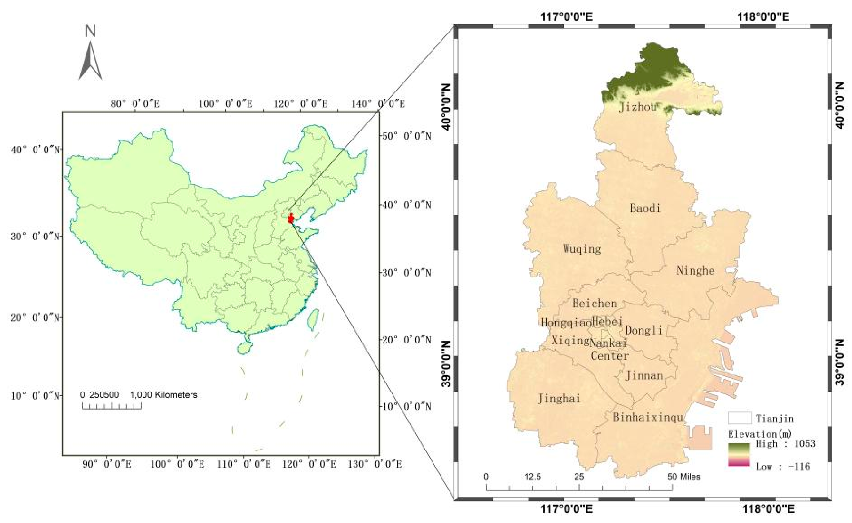
2.1. Overview of the Research Area

Tianjin, a provincial-level administrative region and municipality directly under the Central Government, is a national central city, megacity, and the largest port city in the north of the People’s Republic of China (Figure 1). The terrain of Tianjin mainly consists of plains and depressions, located between 116°43′ and 118°04′ east longitude and between 38°34′ and 40°15′ north latitude, covering a total area of 11,966.45 km². The city center is situated at 117°10′ east longitude and 39°10′ north latitude. Tianjin is divided into 16 districts. In 2022, Tianjin was projected to achieve a regional GDP of CNY 1631.134 billion. At the end of 2022, the total permanent population of Tianjin was 13.63 million. The urbanization rate is 85.11%.

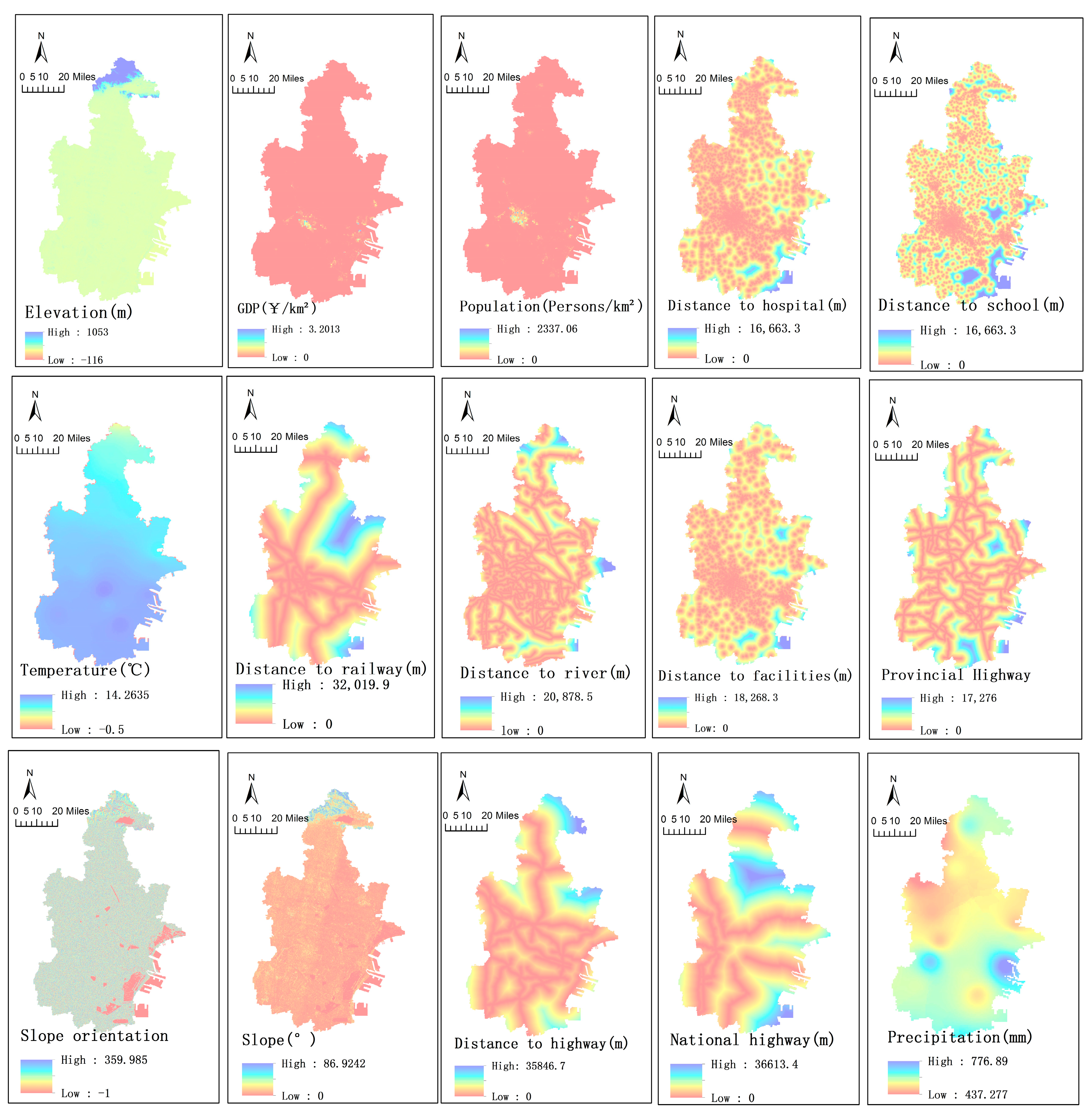
2.2. Research Data Sources

The data and its sources can be found in

Table 1. Data source.

Data Name	Data Source
Land Use DEM, Nighttime Light, Precipitation, Temperature, GDP	RAESADCResource and Environment Science and Data Center (https://www.resdc.cn, accessed on 3 January 2023)
Elevation, Slope, Slope Direction	GDC represented by Geospatial Data Cloud (http://www.gscloud.cn)
Population Density	Worldpop (https://www.worldpop.org, accessed on 3 January 2023)
Distance to Medical Facility Sites, Distance to City Center, Distance to Scientific and Educational Centers, Distance to Railways, Distance to Motorways, Distance to National Highways	ORM represented by Open Road Map database (http://www.openstreetmap.org, accessed on 3 January 2023) calculated using ArcGIS
Energy Consumption Data	Government work: Tianjin Statistical Yearbook (https://stats.tj.gov.cn/tjsj_52032/tjnj/, accessed on 3 January 2023)

. There are a total of15 driving factors, including precipitation, temperature, DEM, etc (Figure 2).

2.3. Research Methods

2.3.1. Research Framework

This article uses the PLUS model to predict multi-scenario land use scenarios in 2030 and combines direct and indirect carbon emissions to accurately calculate the total carbon emissions from 2000 to 2030 in the grid (Figure 3).

2.3.2. PLUS Model

The PLUS model is a patch-level-refined land use prediction model developed on the basis of the FLUS model, which can consider policy-driven and guiding effects. This model develops the LEAS module and CARS module on the basis of the Markov module’s land use demand quantity prediction. This model can not only screen suitable driving factors [25], but also set multi-scenario simulation predictions [26,27,28].

• Markov module

The Markov model can predict future land demand based on the probability matrix of historical land transfer using the following formula:

$$S_{(t+1)}=P_{ij}\times S_{(t)}$$

(1)

In the formula, S_(t+1) represents the land use type at time t + 1, P represents the probability matrix of the land use type transfer, and S represents the land use type at the time t of land use. By changing the transfer probability and setting different development scenarios, future land use needs under different development scenarios are generated as input parameters for the PLUS model to predict the spatial pattern of land use under the ND, ED, and LC scenarios in 2030.

2.

PLUS model

The PLUS model also introduces adaptive inertia coefficients and the same filter matrix to restrict specific land types, and it improves the parameters set for subsequent patch generation. The proposed law of decreasing threshold in the competition process limits specific utilization types, and its expression is as follows:

$$P_{i,K(x)}^{\mathrm{d}}=\frac{{\displaystyle {\sum }_{n=1}^{M}I(h_n(x)=d)}}{M}$$

(2)

where $P_{i,K(x)}^d$ is the integration probability of the spatial unit at the time of transformation to the station type, k; S is the domain weight of the base class, k, at the spatial unit at time, t; and D is the adaptive driving coefficient. Based on previous studies [26,29,30,31], this study mainly selected driving factors from three aspects, including natural factors, social factors, and transportation factors, as well as fifteen driving factors.

“Neighborhood weight” is used to represent the transformation difficulty of different land types. The domain weight values are in the range of [0, 1], and the larger the value, the stronger the expansion ability. The neighborhood weight parameters are shown in

Table 2. Neighborhood weight.

Type of Land	Farmland	Woodland	Grassland	Unutilized Land	Waters	Construction Land
Neighborhood weight	0.6	−0.5	0.4	0.8	0.4	1

.

$$D_k^t=\{\begin{array}{c}{D}_k^{t-1}(G_k^{t-1}\le G_k^{t-1})\\ D_k^{t-1}\times \frac{G_k^{t-2}}{G_k^{t-1}}(0>G_k^{t-2}>G_k^{t-1})\\ D_k^{t-1}\times \frac{G_k^{t-2}}{G_k^{t-1}}(G_k^{t-2}>G_k^{t-1}>0)\end{array}$$

(3)

The transfer matrix is used to define whether conversion occurs between land classes in different regions, where 1 represents conversion being able to occur, and 0 represents restricted conversion. Q1 is the natural development scenario (ND). In this case, the interference of human factors such as national spatial planning is not considered, but historical data are used for the simulation. Q2 is the economic development scenario (ED): Tianjin vigorously developed its economy and expanded its construction land at a rate of nearly two times in the past 20 years [32]. The probability of all land types transferring to construction land is set to increase by 50%, and construction land is not transferred out. Q3 is the low-carbon scenario (LC): Tianjin attaches great importance to ecological protection [33], and the main source of carbon emissions—the expansion of construction land—is reduced by 10%. The probability of transferring all land types to forest land is set at 30%, and forest land will no longer be transferred externally.

Among them, D is the inertia coefficient of site type k at this time, and G_t−1 is the difference between the on-site demand and the actual quantity at t − 1 time.

$$T{P}_k^{d=1,t}\{\begin{array}{c}{P}_k^{d=1}\times (r\times {\mu }_k\times D_k^t({\mathrm{\Omega }}_{i,k}^t=0,r<P_{i,k}^{d=1})\\ P_{i,k}^{d=1}\times {\mathrm{\Omega }}_{i,k}^t\times D_k^t\end{array}$$

(4)

Among them, $T{P}_k^{d=1,t}$ is the comprehensive probability of transitioning to land use types, and R is a random value within (0, 1).

The transition matrix and final site development probability are calculated as follows:

$$\begin{array}{l}if{\displaystyle {\sum }_{k=1}^N\left|G_c^{t-1}\right|}-{\displaystyle {\sum }_{k=1}^N\left|G_c^t\right|}<step,I=I+1\\ \{\begin{array}{c}{P}_{i,c}^{d=1}>\tau ,T{M}_{k,c}=1change\\ P_{i,c}^{d=1}\le \tau ,T{M}_{k,c}=0change\end{array}\tau ={\sigma }^I\times R_1\end{array}$$

(5)

The step size is the step size required to adapt the PLUS model to land use needs; the value of I represents the threshold attenuation steps; δ is between 0 and 1; R₁ is a normal distribution with an average value of 1; and the values of TM_k,c are 0 and 1, indicating whether the land type k defined by the transfer matrix can be converted to c.

The PLUS model verifies the simulation results through Kappa coefficients to ensure its applicability in the Tianjin area. The Kappa coefficient is 0–1, and the closer the value is to 1, the higher the simulation accuracy. When the value exceeds 0.75, it indicates a high simulation accuracy. The simulation accuracy of this article is as high as 0.76, and the comprehensive accuracy is 0.82.

2.3.3. Estimation of Carbon Emissions from Land Use

• Direct carbon emission estimation

The direct carbon emission coefficient method is a technique used to calculate the carbon emissions or carbon absorption of a specific land use type based on its area and corresponding carbon emission coefficient. This method allows for an assessment of how different land use types affect carbon cycling. Previous research has shown that forests, grasslands, water bodies, and unused land have a significant capacity for carbon absorption [34], while cultivated land and construction contribute to carbon emissions. Given the direct impact of changes in land types, such as arable land, forest land, grasslands, water bodies, and unused land, on regional carbon emissions, the carbon emissions of these land types can be estimated using the carbon emission coefficient method. The specific formula for estimation is as follows:

$$C_A={\displaystyle {\sum }_{\mathrm{i}=1}^{\mathrm{n}}(A_i{a}_i)}$$

(6)

In the formula, C_A represents the carbon emissions of different types of land, including arable land, forest land, grassland, water area, and unused land. A represents the area of each land type, and a represents the carbon emission coefficient of each land type. The carbon emission coefficients for arable land, forest land, grassland, water area, and unused land are as follows: 0.422 t (C)·hm⁻², −0.644 t (C)·hm⁻², −0.021 t (C)·hm⁻², −0.005 t (C)·hm⁻², and −0.25 t (C)·hm⁻² [10,13,22,35,36]. These values are based on previous research results and the specific conditions of the study area.

2.

Indirect carbon emission estimation

Due to the complex and diverse utilization methods of construction land, it is difficult to use a unified carbon emission coefficient method to determine carbon emissions. The estimation of carbon emissions from construction land is usually indirectly based on the consumption of fossil fuels used in production and daily life and their carbon emission coefficients [37]. Based on the availability of energy consumption data in a district, coal, coke, crude oil, fuel oil, gasoline, kerosene, diesel, natural gas, and electricity are selected to estimate the carbon emissions of construction land. The specific calculation formula is as follows:

$$C_B={\displaystyle \sum B_i\times {\theta }_i\times {\phi }_i}$$

(7)

In the formula, CB represents the carbon emissions of construction land, and B represents the consumption of fossil fuels. θ denotes the conversion standard coal coefficient, and φ represents the carbon emission coefficient. Among them, the standard coal coefficient and carbon emission coefficient are, respectively, taken from the “China Energy Statistical Yearbook” and the Intergovernmental Panel on Climate Change (IPCC) carbon emission calculation table, as shown in

Table 3. Carbon emission coefficient for each type of energy.

Type of Energy	Conversion Standard Coal Factor (t(C)·t−1)	Carbon Emission Factor (t(C)·t−1)
Coal	0.7143	0.7559
Coke	0.9714	0.855
Crude oil	1.4286	0.5857
Gasoline	1.4714	0.5538
Kerosene	1.4714	0.5714
Diesel oil	1.4571	0.5921
Fuel oil	1.286	0.6185
Natural gas	1.33	0.4483
Electricity power	0.1229	0.2132

.

Based on existing research, it has been found that there is a linear correlation between the number of nighttime lights and energy carbon emissions. Weights were calculated and assigned to each region based on the nighttime lights. To obtain the spatial distribution of construction land lighting, the construction land registration value of 1 was multiplied by the nighttime lighting layer using ArcGIS. The study showed a linear relationship between nighttime lighting and carbon emissions, with a goodness of fit of 0.88. Finally, the carbon emissions of each district are evenly distributed among the 1 km × 1 km patches of construction land, allowing for the construction of an accurate indirect carbon emission intensity coefficient specific to the construction land in each district.

3.

Grid-based estimation of carbon emission intensity

The ArcMap fishing net tool was used to generate a 1 km × 1 km fishing grid for the study area. Carbon emission intensity consists of direct and indirect carbon emission intensity. The formula for calculating the direct carbon emission intensity is as follows: the indirect carbon emission intensity is equal to the carbon emissions of construction land in a certain district or county divided by the number of grids in that district to evenly distribute it to the grid.

$$C={\displaystyle \sum _{i=1}^n\frac{S_{\mathrm{i}}\times {\mathrm{a}}_{\mathrm{i}}}{S}}$$

(8)

In the formula, C is the direct carbon emission intensity, S is the area of the i-th type of land use within the grid, a is the carbon emission coefficient of the i-th type of land use, and S is the total area of the grid, where i includes arable land, forest land, grassland, water area, and unused land.

4.

Carbon Emission Forecast for 2030

The carbon emissions in 2030 from different types of land, such as cultivated land, forest land, grassland, water area, and unused land, were primarily estimated by simulating the future land use area and carbon emission coefficient. To calculate the carbon emissions from construction land, we followed these steps: ①the exponential smoothing method was used to predict the energy consumption of each area in 2030; ②the exponential smoothing method was used to predict the nighttime lighting number of construction land in each area, and this was assigned as a distribution weight to each area [37]. Finally, the carbon emissions from the 1 km × 1 km grid construction land in each district in 2030 were evenly distributed to the grids of each district. The carbon emissions from construction land under the natural development scenario in 2030 served as a benchmark to assign the carbon emissions from the other two scenarios, namely low-carbon development and economic development scenarios.

3. Experimental Results

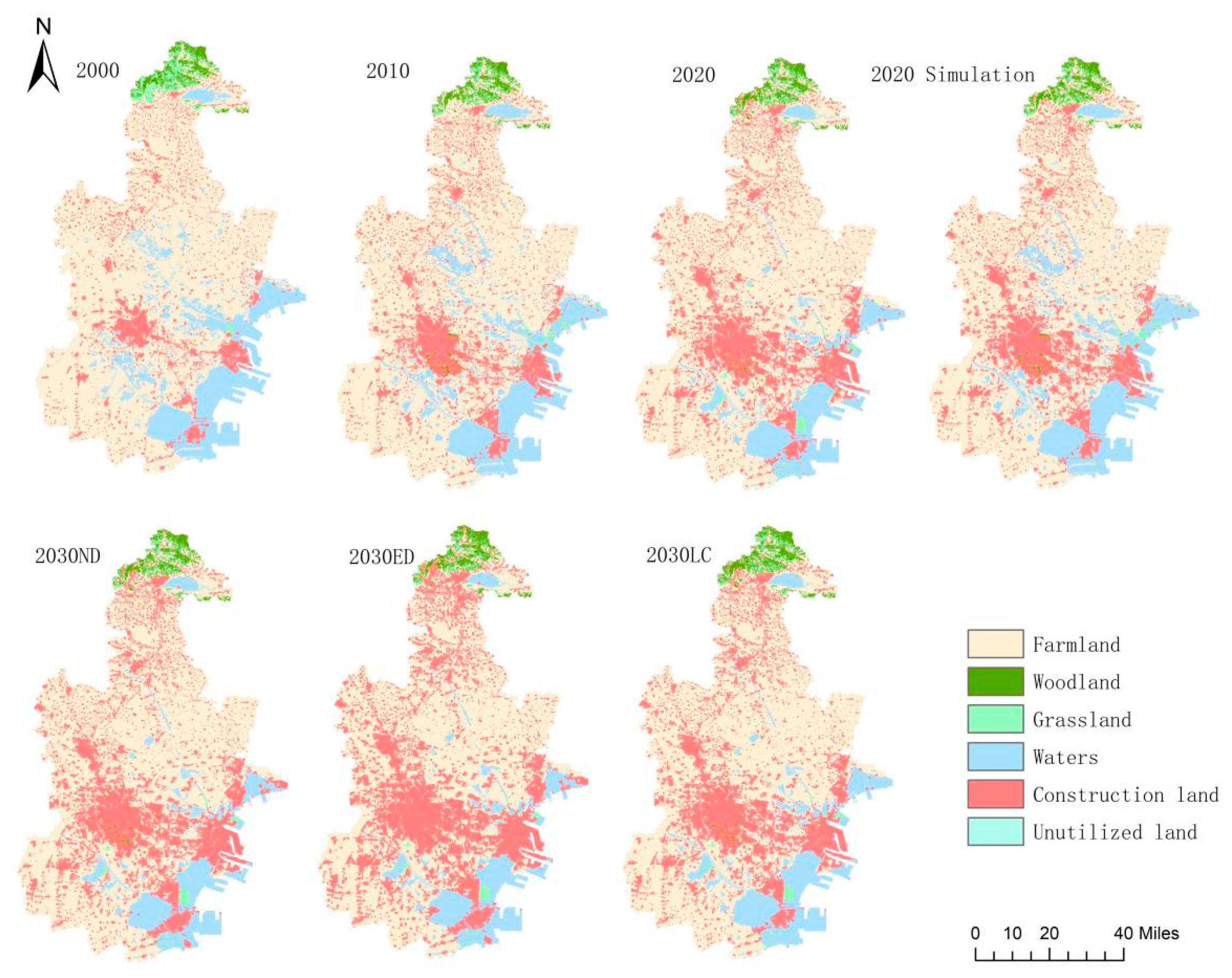
3.1. Spatiotemporal Analysis of Land Use

3.1.1. Analysis of Land Use Time

From 2000 to 2030, there was a significant decrease in the arable land and water areas (Figure 4), and a significant increase in construction land. In the first decade, farmland decreased by 559.4 km² (

Table 4. Land use type area (ND—natural development scenario; ED—economic development scenario; LC—low-carbon scenario).

Landscape Type	Farmland	Woodland	Grassland	Construction Land	Unutilized Land	Water
2000 (km2)	7988.72	204.64	266.67	1365.21	1.11	2107.08
2010 (km2)	7429.32	226.93	220.79	2032.51	1.25	2019.66
2020 (km2)	7228.81	215.90	257.16	2673.49	3.03	1543.18
2030 ED (km2)	6152.93	205.08	227.25	3990.72	2.74	1350.96
2030 ND (km2)	7001.01	214.78	262.96	3194.40	2.94	1275.49
2030 LC (km2)	6971.84	245.46	263.51	3001.89	2.96	1435.92

). In the following decade, the government implemented policies to strictly adhere to the farmland baseline red line, which refers to the minimum area of land that is frequently cultivated, resulting in a decrease of 200.51 km² in farmland reduction. Construction land increased from 1365.21 km² to 2673.49 km², with an average increase of 650 km² every ten years. The speed of urban expansion has remained stable. It is worth noting that in the first decade, forest land in Tianjin increased by 22.29 km² but then decreased by 11.03 km². This is because after the country implemented regional protection, most of the forest land began to be concentrated in the north, and scattered forest land disappeared. The water area decreased from 2107.8 km² to 1543.18 km². This is mainly due to the land reclamation policy in the Binhai New Area (Figure 5), where most of the sea areas have been converted into lad.

In 2030, all three scenarios show trends of a decreasing arable land area and increasing construction land. According to the NDS scenario, farmland was only reduced by 227.80 km², which aligns with the national policy on farmland protection. The construction land increased from 2673.49 km² to 3194.40 km². In the EDS scenario, the construction land increased to 3990.72 km², resulting in a significant reduction in arable land. Lastly, in the LCS scenario, the increase in construction land is the lowest, reaching 3001.89 km².

From 2000 to 2010, there was a significant increase in construction land due to the conversion of water areas. Although there was a decrease in arable land, the conversion of water bodies into cultivated land helped replenish the area of cultivated land. The Tianjin Municipal Government made efforts to convert 39.74 km² of land into grassland and 20.58 km² of cultivated land into forest land. From 2010 to 2020, although some water bodies were converted into arable land, the total amount of arable land still decreased. The main trend during this period was still a significant increase in the area of construction land. Notably, 33.28 km² of grassland was converted into forest land, mainly concentrated in Jizhou District, while scattered forest land in other areas gradually disappeared.

3.1.2. Spatial and Temporal Analysis of Land Use in 2030

In the year 2000, construction land was primarily located in the central districts of the city (Figure 6) (Heping District, Hexi District, Nankai District, Hedong District, Hebei District, and Hongqiao District). Over the next 20 years, it expanded from the city center to the surrounding areas, gradually connecting with the Binhai New Area. This led to the development of Dongli District and Jinnan District in the middle area, resulting in the overall shift of the urban construction land’s center of gravity towards the southeast. The forest land is mainly concentrated in the northern part of Jizhou District, and protecting this forest area in line with national policies will act as a green barrier and contribute to the sustainable development of Tianjin. The reduction in water resources in the Binhai New Area is due to the gradual conversion into construction land, indicating further development in the future.

In different scenarios, the characteristics of the areas vary. In the Binhai New Area, the water area significantly decreased and was then converted into construction land. However, the growth of construction land in other areas has changed relatively little due to limitations on arable land. This gradual connection of construction land between the two economic centers is notable. Furthermore, in Jizhou District, it is evident that the forest land area and grassland area have increased, while the water area is occupied less by construction land. This situation is highly beneficial for the absorption of carbon emissions and provides a valuable reference for the city’s sustainable development plan.

3.2. Spatiotemporal Analysis of Carbon Emissions

3.2.1. Direct Carbon Emission Time Analysis

The direct carbon emissions from 2000 to 2020 were, respectively, 32.27 × 10⁴ t, 29.74 × 10⁴ t, and 28.92 × 10⁴ t, with relatively large forest absorptions of 1.32 × 10⁴ t, 1.46 × 10⁴ t, and 1.39 × 10⁴ t (

Table 5. Direct carbon emissions from land (ND—natural development scenarios; ED—economic development scenario; LC—low-carbon scenario).

Landscape Type (104 t)	Farmland	Woodland	Grassland	Unutilized Land	Water	Direct
2000	33.71	−1.32	−0.06	−0.07	0.00	32.27
2010	31.35	−1.46	−0.05	−0.10	0.00	29.74
2020	30.51	−1.39	−0.05	−0.13	−0.01	28.92
2030 ND	29.54	−1.38	−0.06	−0.16	−0.01	27.94
2030 ED	25.54	−1.32	−0.05	−0.20	−0.01	23.97
2030 LC	29.42	−1.58	−0.06	−0.15	−0.01	27.63

). Under different scenarios in 2030, the minimum absorption of forest land in the economic development scenario was 1.32 × 10⁴ t, with an absorbable value of 1.58 in low-carbon development scenarios × 10⁴ t carbon emissions.

Specifically, Nankai District, Hexi District, Hedong District, and Heping District all exhibit an approximate absorption of 1 ton each. Notably, the Binhai New Area showcases significant carbon absorption capabilities, with recorded values of 56.07 t, 56.85 t, and 26.26 t between 2000 and 2020. The anticipated absorption levels for the year 2030 consist of 24.02 t under a low-carbon model, 3.26 t alongside economic development, and 8.85 t within natural development scenarios. In terms of emissions, the bulk of the emissions originate from Jinghai District due to the concentration of construction land in the central six districts. Consequently, indirect emissions contribute to the majority of carbon emissions, while other land types contribute minimally to absorption.

Areas with high carbon absorption intensity levels are primarily concentrated in the northern part of Jizhou District, Binhai New Area, and the southeastern part of Tianjin City. The northern part of Tianjin acts as a natural barrier, preventing carbon emissions from northern cities like Tianjin and Beijing. In the Binhai New Area, the presence of numerous wetlands and seawater contributes to carbon absorption, providing ecological protection for future economic development in the region (Figure 7).

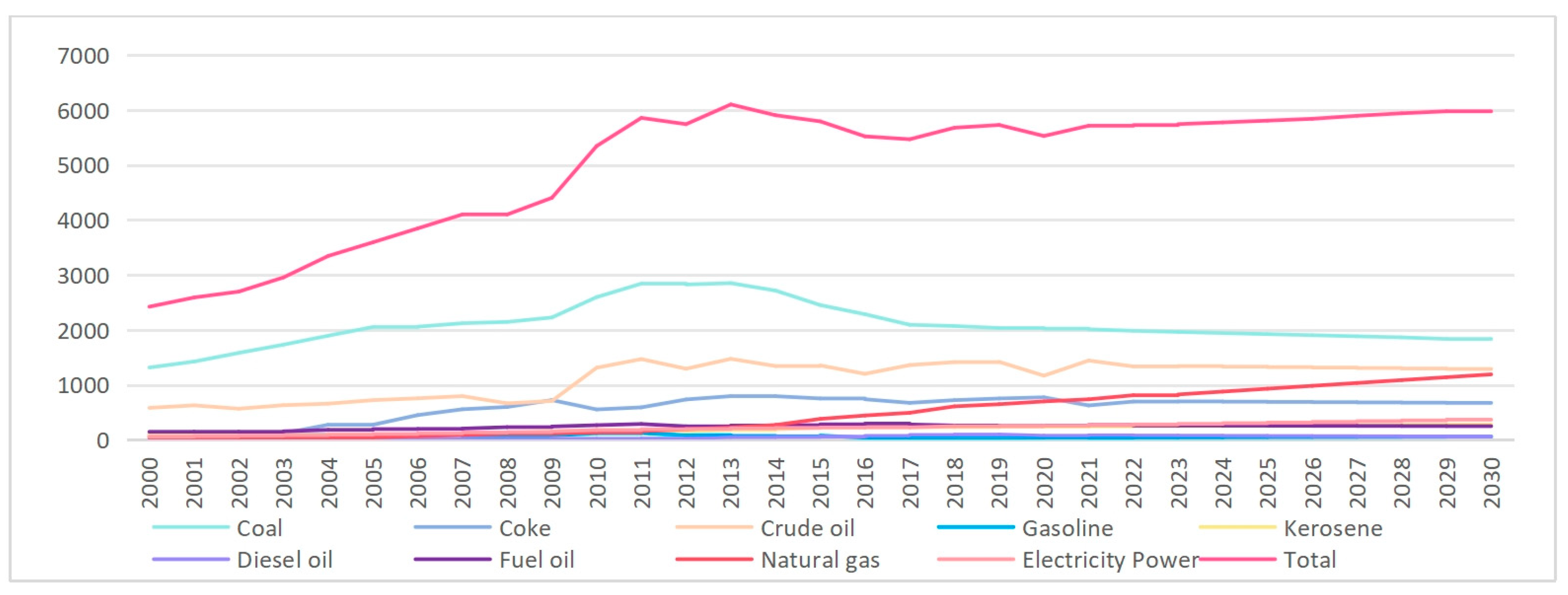
3.2.2. Indirect Carbon Emissions

Due to some missing data, partitioned carbon emission data can be obtained based on nighttime lighting. Based on the nighttime lighting layer and the construction land extraction layer (Figure 8), the nighttime lighting layer of the construction land can be constructed to obtain the nighttime lighting number of the construction land in the partition. A regression model was constructed and found to have a linear relationship with a fitting degree of 0.88. It can be distributed evenly to each grid of construction land, and a unit of a 1 km grid of carbon emissions that is accurate to each year and region was created for construction land.

Based on historical energy consumption data, the exponential smoothing method is used to predict the carbon emissions of energy consumption. Except for the increase in natural gas and electricity consumption, other energy consumption sources have been decreasing year by year, and there has been a marginal decline (Figure 9). As shown in the figure, carbon peaking may be achieved by 2030. Based on the carbon emissions of each 1 km grid in the 2030 natural development scenario, the carbon emissions of the other two scenarios can be inferred, as shown in the following figure (Figure 10).

From 2000 to 2030, the average emission intensity of carbon in Tianjin was measured at 17,734.47 t/km², 26,296.30 t/km², 20,676.04 t/km², and 14,997.13 t/km², respectively. However, certain regions displayed a relatively high emission intensity of construction land, reaching up to three times the average, while in lower regions, it accounted for 66.67% of the average. The trend of carbon emission intensity followed an “initial increase and subsequent decrease” pattern between 2000 and 2020. In 2000, high indirect carbon emissions were predominantly concentrated in the central six districts, ranging from 39,815 t/km² to 25,373.8 t/km². Binhai New Area exhibited concentrations ranging from 10,932.6 t/km² to 14,541.9 t/km², surpassing the carbon emission intensity of all other regions. Overall carbon emissions witnessed a rise in 2010, peaking at 43,161.0 t/km², with the central area mostly exceeding 30,305 t/km². The lower valued area also reached 8550 t/km² to 8646 t/km².

Based on these data, it can be inferred that the rapid urban development during this period necessitated a substantial amount of energy, devoid of government restrictions or the implementation of clean energy technology to manage carbon emissions. In 2020, the overall carbon emissions did not witness a significant decrease, but the carbon emission intensity of construction land notably decreased by 7.5%. Compared to 2010, noticeable reductions in the carbon emission intensity of the Central Six Districts occurred, even surpassing values from 2000. Additionally, Dongli District, Baodi District, and Beichen District achieved significant interdisciplinary reductions in carbon emissions (Figure 9). The only region displaying an increase rather than a reduction was Binhai New Area. Considering the presence of numerous factories (more than 5748 companies) in the Binhai New Area, it is not surprising to find that the growth rate of the carbon emission intensity in this region exceeds that of others.

By 2030, there will be a further reduction in the carbon emission intensity, with the maximum value declining to 40,003 t/km². Analyzing three distinct scenarios for 2030 reveals that the regions with high carbon emission intensity values in EDS exhibited a higher concentration. In the LCS scenario, the protection of forest land in Jizhou District is effectively carried out, and limitations on the expansion of construction land also contribute to the lower carbon emissions.

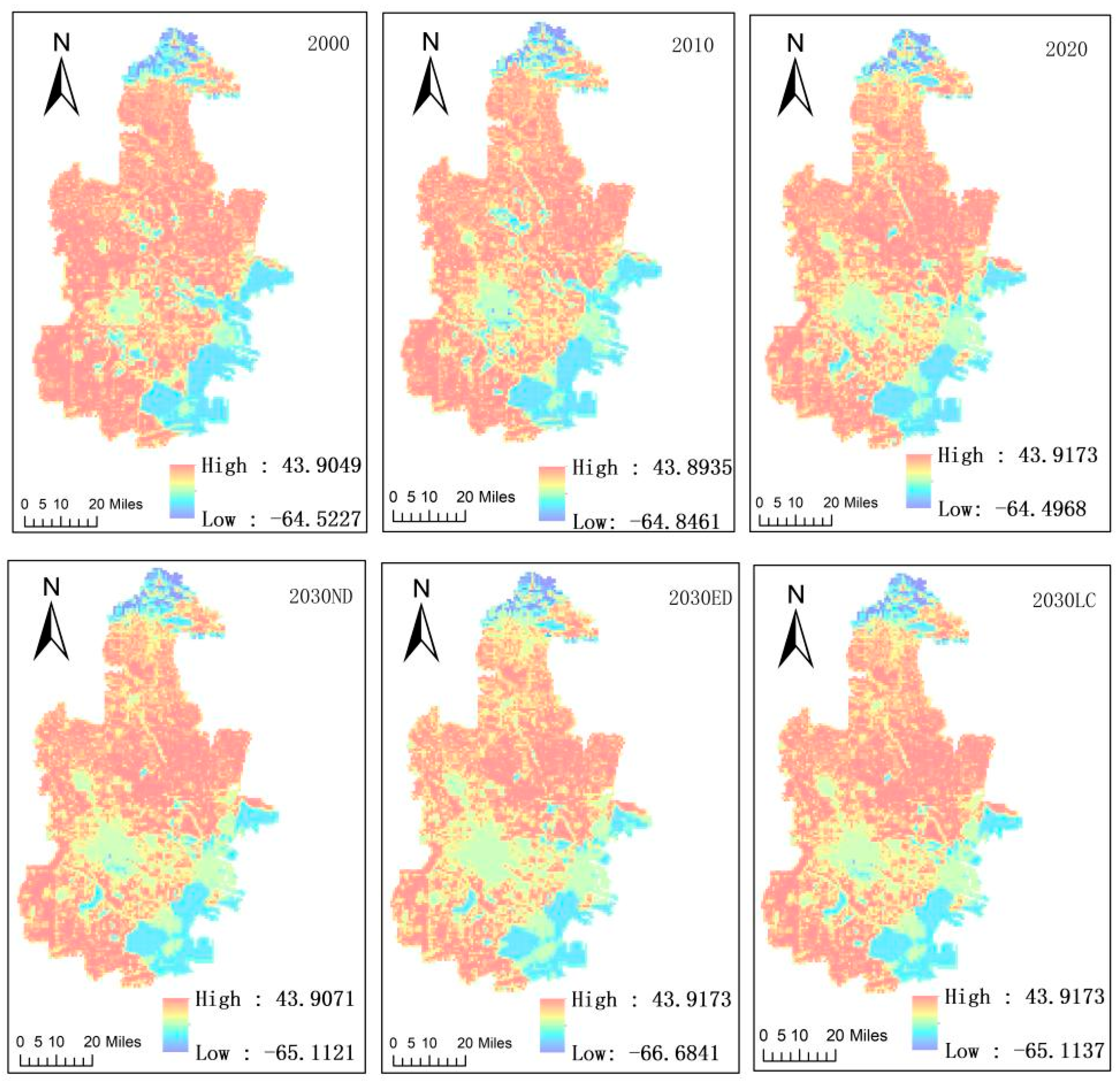
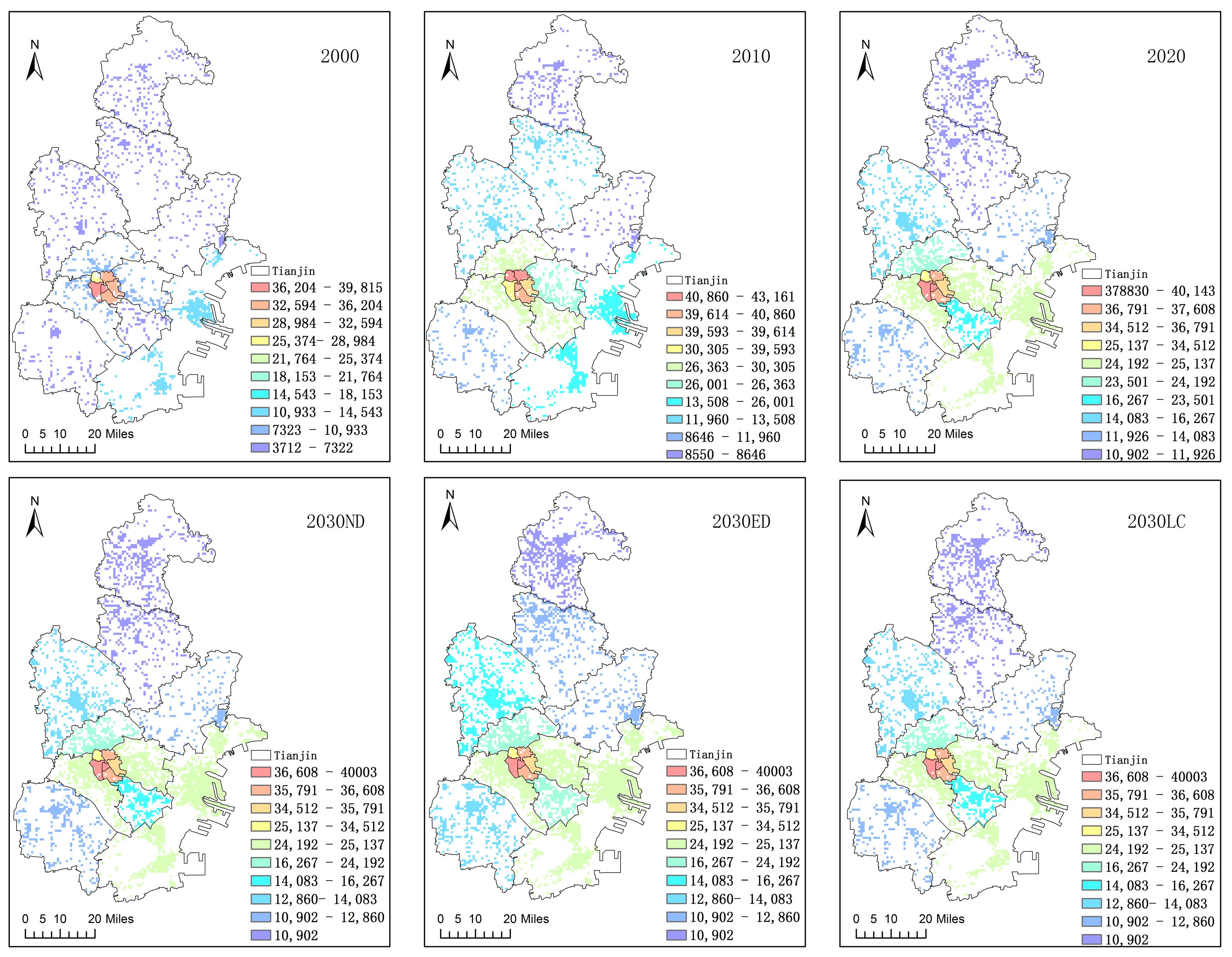
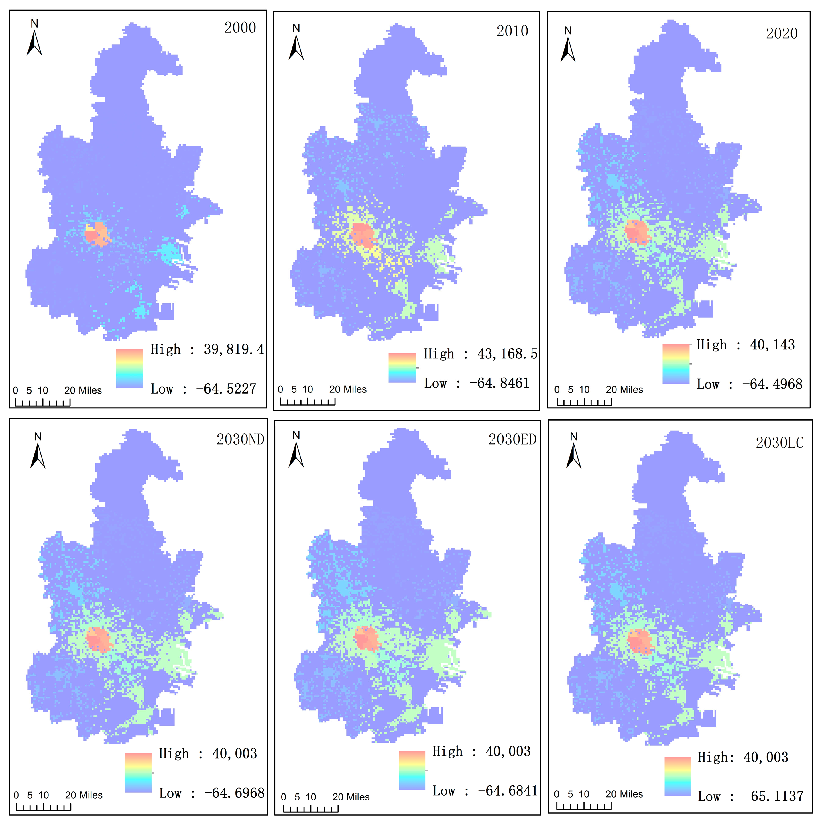
3.2.3. Distribution of Total Carbon Emissions and Carbon Emission Intensity

Based on the statistics of carbon emission intensity in various regions under the natural development scenario in 2030, it can be concluded that the expected emissions under the economic development scenario are 6863.29 × 10⁴ t, and the estimated emissions under the low-carbon development scenario are 5756.80 × 10⁴ t (

Table 6. Direct and indirect carbon emissions (ND—natural development scenario; ED—economic development scenario; LC—low-carbon scenario).

	2000.00	2010.00	2020.00	2030ND	2030ED	2030LD
Direct	32.27	29.74	28.92	27.94	23.97	27.63
Indirect	2421.13	5344.75	5527.72	5984.93	6863.29	5784.43

).

Between 2000 and 2020, the areas with high-intensity total carbon emissions expanded outward from the central six zones. The intensity of these emissions initially showed an increasing trend and then a decreasing trend. Among the four districts, Beichen District, Dongli District, Jinnan District, and Xiqing District, the carbon emission intensity followed a similar pattern. Notably, the overall carbon emission intensity of Binhai New Area has been increasing year by year, making it a focus of government work for future construction.

Under the 2030 natural development scenario, the carbon emission intensity is expected to further decrease. In the economic development scenario, Binhai New Area exhibited the highest carbon emission intensity. Based on the carbon emission intensity quota under the 2030 natural development scenario, the carbon emissions were calculated as follows for the low-carbon development scenario and the economic development scenario (Figure 11).

3.2.4. Analysis of Carbon Emission Intensity Zoning

Based on different carbon emission intensities, this is divided into five levels: highest, higher, medium, lower, and lowest. The highest values of carbon emission intensity are mostly concentrated in the central region, Dongli District, and Xiqing District. Although the overall carbon emission intensity increased in 2010, it decreased overall after 2020. In 2020, Hexi District and Hongqiao District transformed from being highest-value areas to higher-value areas; Dongli District transformed from a higher-value area to a medium-value area. Under the natural development scenario of 2030, Hebei Province will transform from a highest-intensity area to a medium-intensity area. Under the economic development scenario, the overall regional carbon emission intensity increased, while the carbon emission intensities of Xiqing District and Jinghai District increased. In the context of low-carbon development, Hedong District reached a moderate level. Despite the significant increase in construction land in Binhai New Area, its carbon emission intensity level has not changed (Figure 12).

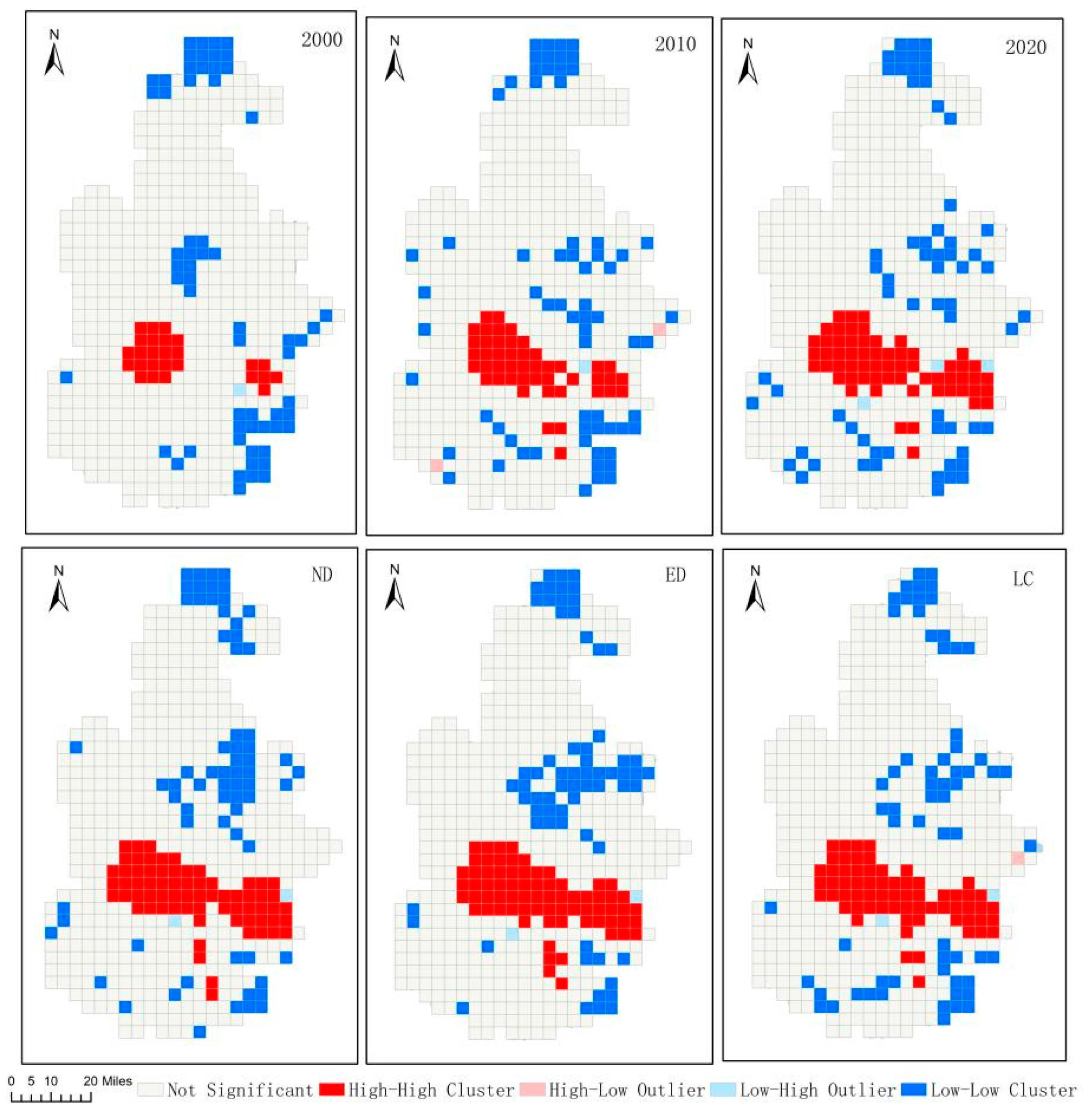
3.2.5. Spatial Autocorrelation Analysis of Carbon Emission Density

The Moran Index is an indicator used to measure geographic spatial patterns and is mainly used to analyze the distribution characteristics of spatial data. The authors calculated the Moran index, and the probability p values are all 0.001. Through the significance test, it is shown that the research correlation is significant and demonstrates positive spatial aggregation characteristics. In order to reveal the local spatial agglomeration change rules of the ecosystem service value in the study area in depth, the average carbon emission intensity was calculated based on 912 grids of 5 km × 5 km, and a LISA (local indicators of spatial association) agglomeration map (Figure 13) was obtained. The city was divided into five different types (high–high clustering, low–low clustering, low–high clustering, high–low clustering, and unimportant). The authors found that the pattern is stable, with high-agglomeration areas concentrated in the six central districts and spreading to the southeast. Low–low agglomeration areas are located in Binhai New Area, Jizhou District, and Ninghe District.

4. Discussion

4.1. Land Use Change and Carbon Emissions

This paper utilizes the PLUS model and examines the relationship between energy consumption carbon emissions and the spatial distribution of future carbon emissions. The findings of this study support the effectiveness of the PLUS model in this type of research [19,20,38]. The results align with those obtained in previous studies, indicating that land use significantly influences carbon emissions [32,39,40,41], and protecting woodlands can help mitigate them [42]. However, this paper introduces a novel approach by accurately calculating carbon emission intensity by district. This study reveals that not all districts experience a decrease in carbon emission intensity when there is an increase in construction land [43,44], such as in the Binhai New Area. A further analysis suggests that the increase in construction land in the Binhai New Area is primarily attributed to the establishment of new factories, which contribute to a higher carbon emission intensity.

4.2. The Relationship between Construction Land Expansion and Carbon Emission Intensity

Based on the research results for carbon emissions from 2000 to 2030 and a spatial cluster analysis, it can be found that the expansion patterns of high carbon emission areas and high-density agglomeration areas are similar. This article speculates that these expansion patterns are affected by the expansion of construction land. Therefore, in order to explore the relationship between construction land and the expansion trend of carbon emission intensity, this paper uses the center of gravity standard deviation ellipse to analyze the migration trajectory of Tianjin’s carbon emission intensity in 2000, 2010, 2020, and 2030 [22,45]. The figure presents the visualization of the center of gravity migration trajectory. The gradual shift of the center of gravity towards the southeast direction from 2000 to 2020 indicates a rapid decrease in carbon emission intensity in the northwest direction. This finding aligns with previous research on the shift of the economic and population centers towards the southeast direction [46]. In the three scenarios for 2030, the economic development scenario exhibits the largest major axis of the ellipse, indicating the widest spatial impact range. The distributions of carbon emission intensity in the low-carbon development and natural development scenarios are relatively similar, with the only difference being a slow northeastward movement of the center of gravity in the low-carbon scenarios. An increase in the radius indicates diffusion, while a decrease in the radius indicates a tendency towards aggregation. The changing trends of the center of gravity of carbon emission intensity and the center of gravity of construction land are highly similar, although their ellipse diameters are different (Figure 14).

4.3. Shortcomings and Prospects

(1) This article aims to develop a carbon emission intensity coefficient for construction land, taking into account the spatial distribution of predicted carbon emissions and carbon emission intensity for construction land expansion. While the coefficient constructed in this study has been accurate for each district of a city, there are still some errors. In the future, it is hoped that a unified coefficient correction method can be identified, incorporating factors such as nighttime lighting, GDP, and population to obtain the carbon emission coefficient specifically for urban exclusive construction land. This will contribute to the advancement of prediction research. Making modifications to the local situation would be more helpful, as it would ensure that this method is more easily scalable and applicable to other cities.

(2) The research results of this article need to be achieved through certain national policies. The research results of this article show that reasonable land use will affect carbon emissions, and combining national spatial planning can achieve this goal. In the future, simulation research can be implemented in reality by combining national spatial planning and extracting restricted areas.

(3) While the results section is exhaustive, delving into the implications of the findings in greater detail, particularly in comparison to existing studies or projections for other urban areas, would be beneficial.

4.4. Policy Recommendations

(1) Fully understanding the concept of demographic dividend and developing appropriate talent policies is crucial. It is worth noting that the population of Tianjin has been experiencing negative growth, and in particular, the permanent population of Binhai New Area has been declining over the years. However, it is important to recognize that an increase in the population density can potentially lead to a reduction in carbon emission intensity [47].

(2) We should promote energy structure reform and accelerate the transformation of industrial structure. Historical data point out that Tianjin’s energy structure has changed, with natural gas and electricity consumption increasing, while the consumption of other energy types decreases; therefore, Tianjin should seize this advantage, make further developments in science and technology, optimize the energy structure, and focus on the use of clean energy to contribute to achieving Tianjin’s “carbon peak” in 2030.

5. Conclusions

(1) Between 2000 and 2020, the area of construction land expanded rapidly by 1308.28 km², representing a growth rate of 95.83% in 2000. This expansion was mainly concentrated in the central six districts. In 2030, the growth of construction land in NDS is projected to reach 3194.40 km². The expansion rate of construction land is similar to that of the previous decade, and the trend remains unchanged in Tianjin. Cultivated land is maintained at 7001.01 km² and has not been excessively encroached upon by the expansion of construction land. On the other hand, EDS is expected to see a growth in construction land to 3990.72 km². Additionally, LCS predicts that forest land will recover to 245.46 km², primarily concentrated in Jizhou District.

(2) From 2000 to 2020, carbon emissions consistently increased annually, with values of 2421.13 × 10⁴ t, 5344.74 × 10⁴ t, and 5527.72 × 10⁴ t, respectively. However, the growth rate of emissions has been gradually declining over time. On the other hand, the Binhai New Area has experienced an upward trend in carbon emission intensity. By 2030, the expected carbon emissions for NDS are projected to reach 6012.87 × 104 t, while EDS is estimated to have emissions of 6863.29 × 10⁴ t, and LCS is estimated to have emissions of 5756.80 × 10⁴ t.

(3) From 2000 to 2020, carbon emission intensity initially rose and then declined, with the highest intensity emissions concentrated in the central six districts. These high intensity emissions have been decreasing year by year. In 2030, there was an overall decrease in emission intensity, with the central six districts showing a trend towards medium emission intensity. Despite the continuous development of the Binhai New Area, its carbon emission intensity still remains in the medium range.

(4) The intensity of carbon emissions decreases as the city size increases. In addition, the agglomeration characteristics of high and low values in the region are both significant and stable.

The expansion trend of areas with high carbon emission intensities, the shift of the center of carbon emission intensity, and the shift of the center of construction land in Tianjin all indicate a movement towards the southeast. However, under the low-carbon development scenario in 2030, the transfer speed of these trends to the southeast is slower. Tianjin’s development follows a low-carbon scenario, suggesting that effective land use planning can help control carbon emissions.

References

1. Avotra, A.A.R.N.; Nawaz, A. Asymmetric impact of transportation on carbon emissions influencing SDGs of climate change. Chemosphere 2023, 324, 138301. [Google Scholar] [CrossRef]
2. Jiang, J.; Xie, D.; Ye, B.; Shen, B.; Chen, Z. Research on China’s cap-and-trade carbon emission trading scheme: Overview and outlook. Appl. Energy 2016, 178, 902–917. [Google Scholar] [CrossRef]
3. Meng, Z.; Wang, H.; Wang, B. Empirical Analysis of Carbon Emission Accounting and Influencing Factors of Energy Consumption in China. Int. J. Environ. Res. Public Health 2018, 15, 2467. [Google Scholar] [CrossRef]
4. Li, J.; Jiao, L.; Li, F.; Lu, X.; Hou, J.; Li, R.; Cai, D. Spatial disequilibrium and influencing factors of carbon emission intensity of construction land in China. J. Clean. Prod. 2023, 396, 136464. [Google Scholar] [CrossRef]
5. Liu, C.; Cheng, L.; Li, J.; Lu, X.; Xu, Y.; Yang, Q. Trade-offs analysis of land use functions in a hilly-mountainous city of northwest Hubei Province: The interactive effects of urbanization and ecological construction. Habitat Int. 2023, 131, 102705. [Google Scholar] [CrossRef]
6. Wang, M.; Wang, Y.; Wu, Y.; Yue, X.; Wang, M.; Hu, P. Identifying the spatial heterogeneity in the effects of the construction land scale on carbon emissions: Case study of the Yangtze River Economic Belt, China. Environ. Res. 2022, 212, 113397. [Google Scholar] [CrossRef]
7. Wu, H.; Deng, K.; Dong, Z.; Meng, X.; Zhang, L.; Jiang, S.; Yang, L.; Xu, Y. Comprehensive assessment of land use carbon emissions of a coal resource-based city, China. J. Clean. Prod. 2022, 379, 134706. [Google Scholar] [CrossRef]
8. Cai, C.; Fan, M.; Yao, J.; Zhou, L.; Wang, Y.; Liang, X.; Liu, Z.; Chen, S. Spatial-temporal characteristics of carbon emissions corrected by socio-economic driving factors under land use changes in Sichuan Province, southwestern China. Ecol. Inform. 2023, 77, 102164. [Google Scholar] [CrossRef]
9. Ke, Y.; Xia, L.; Huang, Y.; Li, S.; Zhang, Y.; Liang, S.; Yang, Z. The carbon emissions related to the land-use changes from 2000 to 2015 in Shenzhen, China: Implication for exploring low-carbon development in megacities. J. Environ. Manag. 2022, 319, 115660. [Google Scholar] [CrossRef] [PubMed]
10. Hong, T.; Huang, X.; Zhang, X.; Deng, X. Correlation modelling between land surface temperatures and urban carbon emissions using multi-source remote sensing data: A case study. Phys. Chem. Earth Parts A/B/C 2023, 132, 103489. [Google Scholar] [CrossRef]
11. Wang, Q.; Yang, C.-h.; Wang, M.-l.; Zhao, L.; Zhao, Y.-c.; Zhang, Q.-p.; Zhang, C.-y. Decoupling analysis to assess the impact of land use patterns on carbon emissions: A case study in the Yellow River Delta efficient eco-economic zone, China. J. Clean. Prod. 2023, 412, 137415. [Google Scholar] [CrossRef]
12. Fu, W.; Yang, S.; Hu, S.; Zhang, P. The impact of embodied land flow in interregional trade on carbon emissions in China. Appl. Geogr. 2023, 159, 103065. [Google Scholar] [CrossRef]
13. Wei, B.; Kasimu, A.; Reheman, R.; Zhang, X.; Zhao, Y.; Aizizi, Y.; Liang, H. Spatiotemporal characteristics and prediction of carbon emissions/absorption from land use change in the urban agglomeration on the northern slope of the Tianshan Mountains. Ecol. Indic. 2023, 151, 110329. [Google Scholar] [CrossRef]
14. Feudjio Fogang, L.; Tiomo, I.F.; Kamga, B.Y.; Mounmemi Kpoumie, H.; Tanougong Nkondjoua, A.D.; Nguetsop, V.F.; Zapfack, L. Predicting land use/land cover changes in the Santchou Wildlife Reserve (Santchou, West-Cameroon) using a CA-Markov model. Trees For. People 2023, 14, 100438. [Google Scholar] [CrossRef]
15. Ghadirian, O.; Lotfi, A.; Moradi, H.; Shetab Boushehri, S.N.; Yousefpour, R. Area-based scenario development in land-use change modeling: A system dynamics-assisted approach for mixed agricultural-residential landscapes. Ecol. Inform. 2023, 76, 102129. [Google Scholar] [CrossRef]
16. Molinero-Parejo, R.; Aguilera-Benavente, F.; Gómez-Delgado, M.; Shurupov, N. Combining a land parcel cellular automata (LP-CA) model with participatory approaches in the simulation of disruptive future scenarios of urban land use change. Comput. Environ. Urban Syst. 2023, 99, 101895. [Google Scholar] [CrossRef]
17. Liang, X.; Guan, Q.; Clarke, K.C.; Liu, S.; Wang, B.; Yao, Y. Understanding the drivers of sustainable land expansion using a patch-generating land use simulation (PLUS) model: A case study in Wuhan, China. Comput. Environ. Urban Syst. 2021, 85, 101569. [Google Scholar] [CrossRef]
18. Luo, H.; Li, Y.; Gao, X.; Meng, X.; Yang, X.; Yan, J. Carbon emission prediction model of prefecture-level administrative region: A land-use-based case study of Xi’an city, China. Appl. Energy 2023, 348, 121488. [Google Scholar] [CrossRef]
19. Rong, T.; Zhang, P.; Li, G.; Wang, Q.; Zheng, H.; Chang, Y.; Zhang, Y. Spatial correlation evolution and prediction scenario of land use carbon emissions in the Yellow River Basin. Ecol. Indic. 2023, 154, 110701. [Google Scholar] [CrossRef]
20. Rong, T.; Zhang, P.; Zhu, H.; Jiang, L.; Li, Y.; Liu, Z. Spatial correlation evolution and prediction scenario of land use carbon emissions in China. Ecol. Inform. 2022, 71, 101802. [Google Scholar] [CrossRef]
21. Plevin, R.J.; Jones, J.; Kyle, P.; Levy, A.W.; Shell, M.J.; Tanner, D.J. Choices in land representation materially affect modeled biofuel carbon intensity estimates. J. Clean. Prod. 2022, 349, 131477. [Google Scholar] [CrossRef] [PubMed]
22. Gui, D.; He, H.; Liu, C.; Han, S. Spatio-temporal dynamic evolution of carbon emissions from land use change in Guangdong Province, China, 2000–2020. Ecol. Indic. 2023, 156, 111131. [Google Scholar] [CrossRef]
23. Li, W.; Chen, Z.; Li, M.; Zhang, H.; Li, M.; Qiu, X.; Zhou, C. Carbon emission and economic development trade-offs for optimizing land-use allocation in the Yangtze River Delta, China. Ecol. Indic. 2023, 147, 109950. [Google Scholar] [CrossRef]
24. The Tianjin Carbon Peak Implementation Plan was recently released. China Chlor-Alkali, 2022; 50.
25. Chen, S.; Yao, S. Identifying the drivers of land expansion and evaluating multi-scenario simulation of land use: A case study of Mashan County, China. Ecol. Inform. 2023, 77, 102201. [Google Scholar] [CrossRef]
26. Gao, L.; Tao, F.; Liu, R.; Wang, Z.; Leng, H.; Zhou, T. Multi-scenario simulation and ecological risk analysis of land use based on the PLUS model: A case study of Nanjing. Sustain. Cities Soc. 2022, 85, 104055. [Google Scholar] [CrossRef]
27. Liu, Y.; Jing, Y.; Han, S. Multi-scenario simulation of land use/land cover change and water yield evaluation coupled with the GMOP-PLUS-InVEST model: A case study of the Nansi Lake Basin in China. Ecol. Indic. 2023, 155, 110926. [Google Scholar] [CrossRef]
28. Shi, Q.; Gu, C.-J.; Xiao, C. Multiple scenarios analysis on land use simulation by coupling socioeconomic and ecological sustainability in Shanghai, China. Sustain. Cities Soc. 2023, 95, 104578. [Google Scholar] [CrossRef]
29. Li, X.; Fu, J.; Jiang, D.; Lin, G.; Cao, C. Land use optimization in Ningbo City with a coupled GA and PLUS model. J. Clean. Prod. 2022, 375, 134004. [Google Scholar] [CrossRef]
30. Wang, M.; Jiang, Z.; Li, T.; Yang, Y.; Jia, Z. Analysis on absolute conflict and relative conflict of land use in Xining metropolitan area under different scenarios in 2030 by PLUS and PFCI. Cities 2023, 137, 104314. [Google Scholar]
31. Zhang, Z.; Hu, B.; Jiang, W.; Qiu, H. Spatial and temporal variation and prediction of ecological carrying capacity based on machine learning and PLUS model. Ecol. Indic. 2023, 154, 110611. [Google Scholar] [CrossRef]
32. Zhou, Y.; Chen, M.; Tang, Z.; Mei, Z. Urbanization, land use change, and carbon emissions: Quantitative assessments for city-level carbon emissions in Beijing-Tianjin-Hebei region. Sustain. Cities Soc. 2021, 66, 102701. [Google Scholar] [CrossRef]
33. Long, H.; Yuan, L.; Yin, Z.; Wu, X. Spatiotemporal of ecosystem service values response to land use/cover change based on geo-informatic Tupu—A case study in Tianjin, China. Ecol. Indic. 2023, 154, 110511. [Google Scholar] [CrossRef]
34. Escolano-Moltó, A.; Flecha, S.; Vaquer-Sunyer, R.; Wesselmann, M.; Marbà, N.; Hendriks, I.E. Mediterranean Seagrasses as Carbon Sinks: Methodological and Regional Differences; Copernicus GmbH: Göttingen, Germany, 2021. [Google Scholar]
35. Zu-Cong, C.; Guo-Ding, K.; Tsuruta, H.; Mosier, A. Estimate of CH4 Emissions from Year-Round Flooded Rice Fields During Rice Growing Season in China. Pedosphere 2005, 15, 66–71. [Google Scholar]
36. Yang, X.; Liu, X. Path analysis and mediating effects of influencing factors of land use carbon emissions in Chang-Zhu-Tan urban agglomeration. Technol. Forecast. Soc. Chang. 2023, 188, 122268. [Google Scholar] [CrossRef]
37. Wang, M.; Wang, Y.; Teng, F.; Ji, Y. The spatiotemporal evolution and impact mechanism of energy consumption carbon emissions in China from 2010 to 2020 by integrating multisource remote sensing data. J. Environ. Manag. 2023, 346, 119054. [Google Scholar] [CrossRef] [PubMed]
38. Yang, Y.; Wang, H.; Li, X.; Huang, X.; Lyu, X.; Tian, H.; Qu, T. How will ecosystem carbon sequestration contribute to the reduction of regional carbon emissions in the future? analysis based on the MOP-PLUS model framework. Ecol. Indic. 2023, 156, 111156. [Google Scholar] [CrossRef]
39. Chen, W.; Gu, T.; Fang, C.; Zeng, J. Global urban low-carbon transitions: Multiscale relationship between urban land and carbon emissions. Environ. Impact Assess. Rev. 2023, 100, 107076. [Google Scholar] [CrossRef]
40. Liu, J.; Peng, K.; Zuo, C.; Li, Q. Spatiotemporal variation of land-use carbon emissions and its implications for low carbon and ecological civilization strategies: Evidence from Xiamen-Zhangzhou-Quanzhou metropolitan circle, China. Sustain. Cities Soc. 2022, 86, 104083. [Google Scholar] [CrossRef]
41. Wu, H.; Fang, S.; Zhang, C.; Hu, S.; Nan, D.; Yang, Y. Exploring the impact of urban form on urban land use efficiency under low-carbon emission constraints: A case study in China’s Yellow River Basin. J. Environ. Manag. 2022, 311, 114866. [Google Scholar] [CrossRef]
42. Guo, Y.; Ren, Z.; Wang, C.; Zhang, P.; Ma, Z.; Hong, S.; Hong, W.; He, X. Spatiotemporal patterns of urban forest carbon sequestration capacity: Implications for urban CO2 emission mitigation during China’s rapid urbanization. Sci. Total Environ. 2024, 912, 168781. [Google Scholar] [CrossRef]
43. Song, C.; Yang, J.; Wu, F.; Xiao, X.; Xia, J.; Li, X. Response characteristics and influencing factors of carbon emissions and land surface temperature in Guangdong Province, China. Urban Clim. 2022, 46, 101330. [Google Scholar] [CrossRef]
44. Wang, Y.; Fan, H.; Wang, H.; Che, Y.; Wang, J.; Liao, Y.; Lv, S. High-carbon expansion or low-carbon intensive and mixed land-use? Recent observations from megacities in developing countries: A case study of Shanghai, China. J. Environ. Manag. 2023, 348, 119294. [Google Scholar] [CrossRef]
45. Zhang, L.; Hu, B.; Zhang, Z.; Liang, G. Research on the spatiotemporal evolution and mechanism of ecosystem service value in the mountain-river-sea transition zone based on “production-living-ecological space”—Taking the Karst-Beibu Gulf in Southwest Guangxi, China as an example. Ecol. Indic. 2023, 148, 109889. [Google Scholar] [CrossRef]
46. Xiao, F.; Chen, G.; Jiang, J. The Impact of the Establishment of National New Area on the Migration of Regional Center of Gravity: Taking Tianjin Binhai New Area as an Example. In Proceedings of the 2015 China Urban Planning Annual Conference, Guiyang, China, 19–21 September 2015; p. 11. [Google Scholar]
47. Yan, Y.; Huang, J. The role of population agglomeration played in China’s carbon intensity: A city-level analysis. Energy Econ. 2022, 114, 106276. [Google Scholar] [CrossRef]
Figure 1. Study area of Tianjin.
Land 12 02160 g001
Figure 2. Driving factors.
Land 12 02160 g002
Figure 3. Research framework (ND—natural development scenarios; ED—economic development scenario; LC—low-carbon scenario).
Land 12 02160 g003
Figure 4. Land use data (ND—natural development scenarios; ED—economic development scenario; LC—low-carbon scenario). (a) Statistical map of land area; (b) chordal maps of land transfer from 2000 to 2010; (c) chordal maps of land transfer from 2010 to 2020.
Land 12 02160 g004
Figure 5. Results for land use in Tianjin between 2000 and 2030 (ND—natural development scenario; ED—economic development scenario; LC—low-carbon scenario).
Land 12 02160 g005
Figure 6. Detailed area map of the six central districts.
Land 12 02160 g006
Figure 7. The spatial distribution results for direct land carbon emission intensity (10−2 t/km2) (ND—natural development scenario; ED—economic development scenario; LC—low-carbon scenario).
Land 12 02160 g007
Figure 8. Nighttime light data from 2000 to 2020.
Land 12 02160 g008
Figure 9. Energy consumption prediction.
Land 12 02160 g009
Figure 10. The spatial distribution results for indirect land carbon emission intensity (t/km2) (ND—natural development scenario; ED—economic development scenario; LC—low-carbon scenario).
Land 12 02160 g010
Figure 11. The spatial distribution results for total land carbon emission intensity (t/km2) (ND—natural development scenario; ED—economic development scenario; LC—low-carbon scenario).
Land 12 02160 g011
Figure 12. Carbon emission intensity level diagram (ND—natural development scenario; ED—economic development scenario; LC—low-carbon scenario).
Land 12 02160 g012
Figure 13. LISA agglomeration map showing carbon emission intensity from 2000 to 2030 (ND—natural development scenario; ED—economic development scenario; LC—low-carbon scenario).
Land 12 02160 g013
Figure 14. (a) Carbon emission intensity center of gravity transfer diagram. (b) Construction land center of gravity transfer diagram (ND—natural development scenario; ED—economic development scenario; LC—low-carbon scenario).
Land 12 02160 g014