
Determination of Spatial Pattern of Environmental Consequences of Dams in Watersheds


Abstract
:1. Introduction
2. Study Area and Materials
2.1. Study Area
2.2. Materials
2.2.1. Watershed
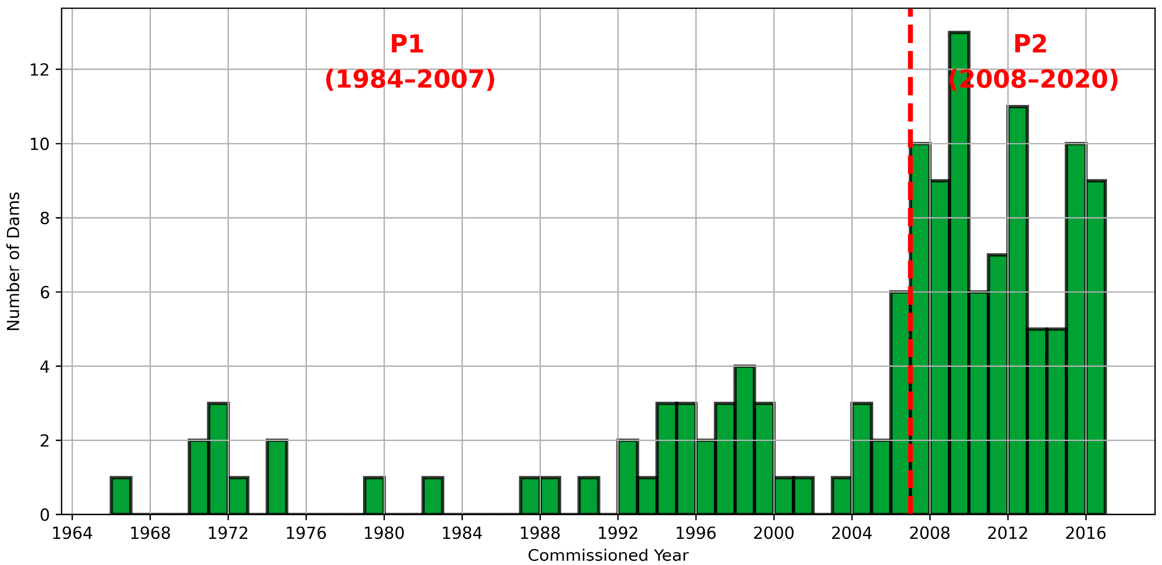
2.2.2. Dams
2.2.3. Wetlands
2.2.4. Water-Inundated Areas of Wetlands
2.2.5. Precipitation Data
3. Methods
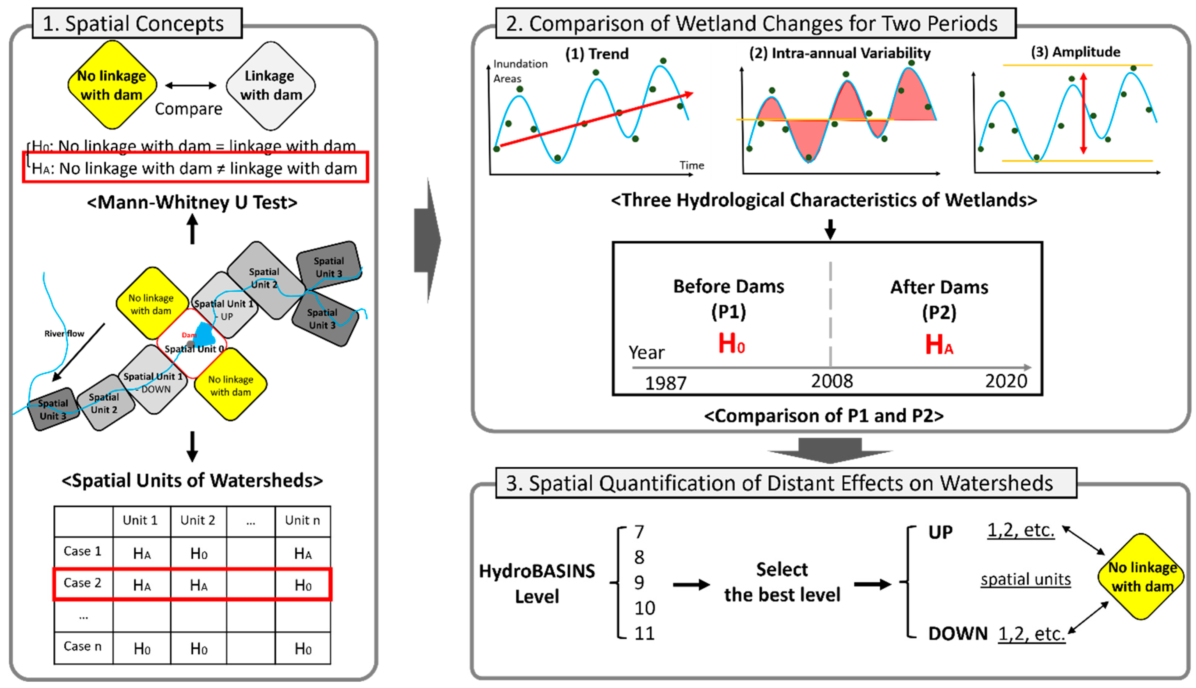
3.1. Hydrological Characteristics of Wetlands from Monthly Inundation Areas
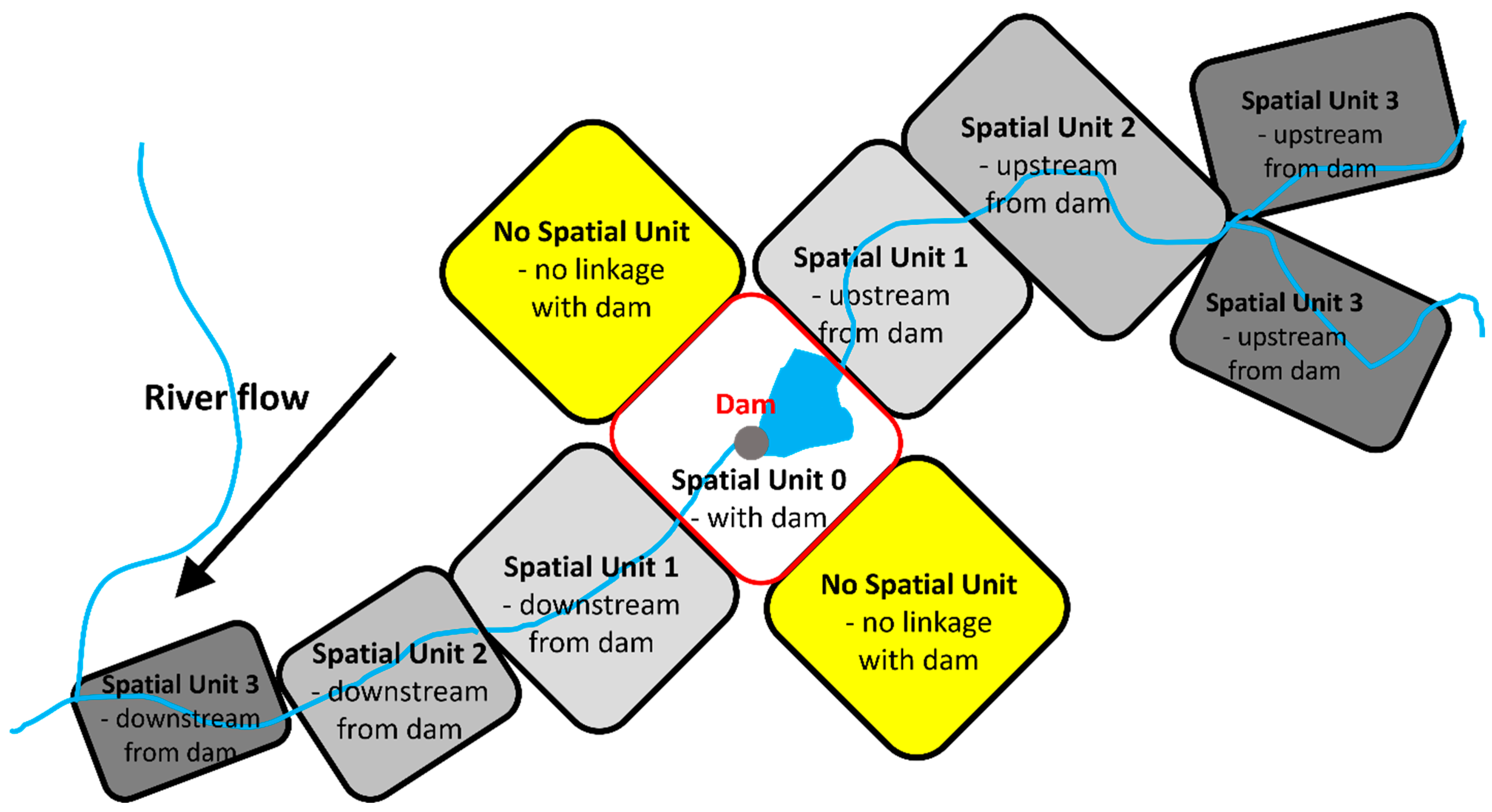
3.2. Pfafstetter Codes: Determination of the Location of Wetlands Regarding the Dam Placement
- If the digit for the last number of digits is odd,
- Upstream: the watersheds with Pfafstetter code having the larger number for the last number of digits.
- Downstream: the watersheds with Pfafstetter code having the smaller odd number for the last number of digits.
- If the digit for the last number of digits is even,
- Upstream: all sub-watersheds will be upstream (i.e., watersheds with the lower watershed level will be upstream).
- Downstream: the watersheds with Pfafstetter code having the smaller odd number for the last number of digits.
- If the digit for the last number of digits is 0: Skip this.
3.3. Spatial Units for Watersheds
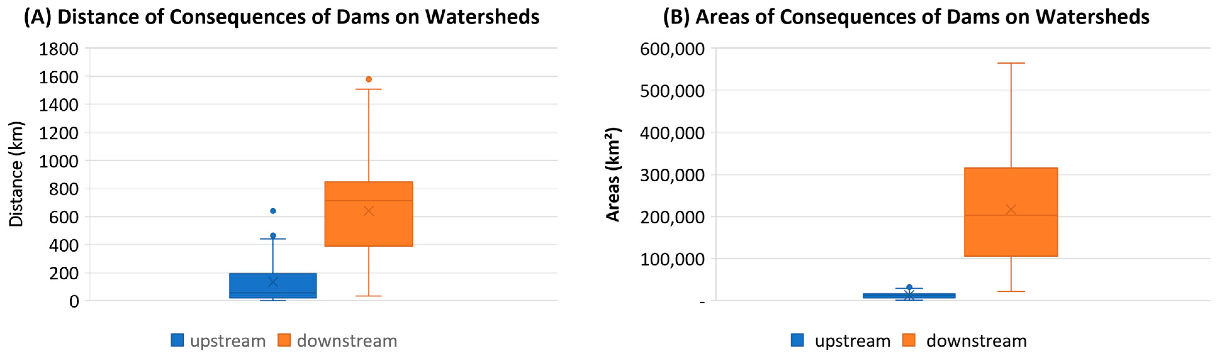
3.4. Quantification of Spatial Pattern of Dam Results on Watersheds
3.5. Investigation of Influence of Climate Variability on the Inundation
4. Results
4.1. Mann–Whitney U Tests for Various Levels and Spatial Units
4.2. Correlation Analysis between Precipitation and Inundation Areas
5. Discussion
6. Conclusions
Author Contributions
Funding
Data Availability Statement
Conflicts of Interest
References
- Mulligan, M.; van Soesbergen, A.; Sáenz, L. GOODD, a Global Dataset of More than 38,000 Georeferenced Dams. Sci. Data 2020, 7, 31. [Google Scholar] [CrossRef] [PubMed]
- Fan, P.; Cho, M.S.; Lin, Z.; Ouyang, Z.; Qi, J.; Chen, J.; Moran, E.F. Recently Constructed Hydropower Dams Were Associated with Reduced Economic Production, Population, and Greenness in Nearby Areas. Proc. Natl. Acad. Sci. USA 2022, 119, e2108038119. [Google Scholar] [CrossRef]
- Poff, N.L.R.; Schmidt, J.C. How Dams Can Go with the Flow. Science 2016, 353, 1099–1100. [Google Scholar] [CrossRef] [PubMed]
- Chen, G.; Powers, R.P.; Carvalho, L.M.T.D.; Mora, B. Spatiotemporal Patterns of Tropical Deforestation and Forest Degradation in Response to the Operation of the Tucuruí Hydroelectricdam in the Amazon Basin. Appl. Geogr. 2015, 63, 1–8. [Google Scholar] [CrossRef]
- Han, X.; Feng, L.; Hu, C.; Chen, X. Wetland Changes of China’s Largest Freshwater Lake and Their Linkage with the Three Gorges Dam. Remote Sens. Environ. 2018, 204, 799–811. [Google Scholar] [CrossRef]
- Ezcurra, E.; Barrios, E.; Ezcurra, P.; Ezcurra, A.; Vanderplank, S.; Vidal, O.; Villanueva-Almanza, L.; Aburto-Oropeza, O. A Natural Experiment Reveals the Impact of Hydroelectric Dams on the Estuaries of Tropical Rivers. Sci. Adv. 2019, 5, aau9875. [Google Scholar] [CrossRef]
- Tullos, D. Assessing the Influence of Environmental Impact Assessments on Science and Policy: An Analysis of the Three Gorges Project. J. Environ. Manag. 2009, 90, S208–S223. [Google Scholar] [CrossRef]
- Tilt, B.; Braun, Y.; He, D. Social Impacts of Large Dam Projects: A Comparison of International Case Studies and Implications for Best Practice. J. Environ. Manag. 2009, 90, S249–S257. [Google Scholar] [CrossRef]
- Winemiller, K.O.; McIntyre, P.B.; Castello, L.; Fluet-Chouinard, E.; Giarrizzo, T.; Nam, S.; Baird, I.G.; Darwall, W.; Lujan, N.K.; Harrison, I.; et al. Balancing Hydropower and Biodiversity in the Amazon, Congo, and Mekong. Science 2016, 351, 128–129. [Google Scholar] [CrossRef]
- Baird, I.G.; Silvano, R.A.M.; Parlee, B.; Poesch, M.; Maclean, B.; Napoleon, A.; Lepine, M.; Hallwass, G. The Downstream Impacts of Hydropower Dams and Indigenous and Local Knowledge: Examples from the Peace–Athabasca, Mekong, and Amazon. Environ. Manag. 2021, 67, 682–696. [Google Scholar] [CrossRef]
- Cho, M.S.; Qi, J. Quantifying Spatiotemporal Impacts of Hydro-Dams on Land Use / Land Cover Changes in the Lower Mekong River Basin. Appl. Geogr. 2021, 136, 102588. [Google Scholar] [CrossRef]
- Abrial, E.; Lorenzón, R.E.; Rabuffetti, A.P.; Blettler, M.C.M.; Espínola, L.A. Hydroecological Implication of Long-Term Flow Variations in the Middle Paraná River Floodplain. J. Hydrol. 2021, 603, 126957. [Google Scholar] [CrossRef]
- Ouyang, W.; Shan, Y.; Hao, F.; Shi, X.; Wang, X. Accumulated Impact Assessment of River Buffer Zone after 30 Years of Dam Disturbance in the Yellow River Basin. Stoch. Environ. Res. Risk Assess. 2013, 27, 1069–1079. [Google Scholar] [CrossRef]
- Cho, M.S.; Qi, J. Characterization of the Impacts of Hydro-Dams on Wetland Inundations in Southeast Asia. Sci. Total Environ. 2023, 864, 160941. [Google Scholar] [CrossRef]
- Han, Z.; Long, D.; Fang, Y.; Hou, A.; Hong, Y. Impacts of Climate Change and Human Activities on the Flow Regime of the Dammed Lancang River in Southwest China. J. Hydrol. 2019, 570, 96–105. [Google Scholar] [CrossRef]
- Lu, X.X.; Li, S.; Kummu, M.; Padawangi, R.; Wang, J.J. Observed Changes in the Water Flow at Chiang Saen in the Lower Mekong: Impacts of Chinese Dams? Quat. Int. 2014, 336, 145–157. [Google Scholar] [CrossRef]
- Poff, N.L.R.; Olden, J.D.; Merritt, D.M.; Pepin, D.M. Homogenization of Regional River Dynamics by Dams and Global Biodiversity Implications. Proc. Natl. Acad. Sci. USA 2007, 104, 5732–5737. [Google Scholar] [CrossRef]
- Chaudhari, S.; Pokhrel, Y. Alteration of River Flow and Flood Dynamics by Existing and Planned Hydropower Dams in the Amazon River Basin. Water Resour. Res. 2022, 58, e2021WR030555. [Google Scholar] [CrossRef]
- Bussi, G.; Darby, S.E.; Whitehead, P.G.; Jin, L.; Dadson, S.J.; Voepel, H.E.; Vasilopoulos, G.; Hackney, C.R.; Hutton, C.; Berchoux, T.; et al. Impact of Dams and Climate Change on Suspended Sediment Flux to the Mekong Delta. Sci. Total Environ. 2021, 755, 142468. [Google Scholar] [CrossRef]
- Zheng, Y.; Zhang, G.; Wu, Y.; Xu, Y.J.; Dai, C. Dam Effects on Downstream Riparian Wetlands: The Nenjiang River, Northeast China. Water 2019, 11, 2038. [Google Scholar] [CrossRef]
- Salmivaara, A.; Kummu, M.; Keskinen, M. Using Global Datasets to Create Environmental Profiles for Data-Poor Regions: A Case from the Irrawaddy and Salween River Basins. Environ. Manag. 2013, 51, 897–911. [Google Scholar] [CrossRef]
- Bonnema, M.; Hossain, F. Assessing the Potential of the Surface Water and Ocean Topography Mission for Reservoir Monitoring in the Mekong River Basin. Water Resour. Res. 2019, 55, 444–461. [Google Scholar] [CrossRef]
- Dang, T.D.; Cochrane, T.A.; Arias, M.E.; Van, P.D.T.; de Vries, T.T. Hydrological Alterations from Water Infrastructure Development in the Mekong Floodplains. Hydrol. Process. 2016, 30, 3824–3838. [Google Scholar] [CrossRef]
- Erwin, K.L. Wetlands and Global Climate Change: The Role of Wetland Restoration in a Changing World. Wetl. Ecol. Manag. 2009, 17, 71–84. [Google Scholar] [CrossRef]
- Ekumah, B.; Armah, F.A.; Afrifa, E.K.A.; Aheto, D.W.; Odoi, J.O.; Afitiri, A.-R. Assessing Land Use and Land Cover Change in Coastal Urban Wetlands of International Importance in Ghana Using Intensity Analysis. Wetl. Ecol. Manag. 2020, 28, 271–284. [Google Scholar] [CrossRef]
- Wang, J.; Sheng, Y.; Tong, T.S.D. Monitoring Decadal Lake Dynamics across the Yangtze Basin Downstream of Three Gorges Dam. Remote Sens. Environ. 2014, 152, 251–269. [Google Scholar] [CrossRef]
- Arias, M.E.; Cochrane, T.A.; Piman, T.; Kummu, M.; Caruso, B.S.; Killeen, T.J. Quantifying Changes in Flooding and Habitats in the Tonle Sap Lake (Cambodia) Caused by Water Infrastructure Development and Climate Change in the Mekong Basin. J. Environ. Manag. 2012, 112, 53–66. [Google Scholar] [CrossRef]
- Middleton, B.A.; Souter, N.J. Functional Integrity of Freshwater Forested Wetlands, Hydrologic Alteration, and Climate Change. Ecosyst. Health Sustain. 2016, 2, e01200. [Google Scholar] [CrossRef]
- Kirchherr, J.; Pohlner, H.; Charles, K.J. Cleaning up the Big Muddy: A Meta-Synthesis of the Research on the Social Impact of Dams. Environ. Impact Assess. Rev. 2016, 60, 115–125. [Google Scholar] [CrossRef]
- Timpe, K.; Kaplan, D. The Changing Hydrology of a Dammed Amazon. Sci. Adv. 2017, 3, e1700611. [Google Scholar] [CrossRef]
- Piman, T.; Cochrane, T.A.; Arias, M.E.; Green, A.; Dat, N.D. Assessment of Flow Changes from Hydropower Development and Operations in Sekong, Sesan, and Srepok Rivers of the Mekong Basin. J. Water Resour. Plan. Manag. 2013, 139, 723–732. [Google Scholar] [CrossRef]
- Ziv, G.; Baran, E.; Nam, S.; Rodriguez-Iturbe, I.; Levin, S.A. Trading-off Fish Biodiversity, Food Security, and Hydropower in the Mekong River Basin. Proc. Natl. Acad. Sci. USA 2012, 109, 5609–5614. [Google Scholar] [CrossRef]
- Robinson, R.A.J.; Bird, M.I.; Nay, W.O.; Hoey, T.B.; Maung, M.A.; Higgitt, D.L.; Lu, X.X.; Aung, S.; Tin, T.; Swe, L.W. The Irrawaddy River Sediment Flux to the Indian Ocean: The Original Nineteenth-Century Data Revisited. J. Geol. 2007, 115, 629–640. [Google Scholar] [CrossRef]
- WLE. Dataset on the Dams of the Irrawaddy, Mekong, Red and Salween River Basins; WLE: Sydney, Australia, 2017. [Google Scholar]
- Schmitt, R.J.P.; Bizzi, S.; Castelletti, A.; Kondolf, G.M. Improved Trade-Offs of Hydropower and Sand Connectivity by Strategic Dam Planning in the Mekong. Nat. Sustain. 2018, 1, 96–104. [Google Scholar] [CrossRef]
- Soukhaphon, A.; Baird, I.G.; Hogan, Z.S. The Impacts of Hydropower Dams in the Mekong River Basin: A Review. Water 2021, 13, 265. [Google Scholar] [CrossRef]
- Fearnside, P.M. Environmental and Social Impacts of Hydroelectric Dams in Brazilian Amazonia: Implications for the Aluminum Industry. World Dev. 2016, 77, 48–65. [Google Scholar] [CrossRef]
- Xu, J.; Grumbine, R.E.; Beckschäfer, P. Landscape Transformation through the Use of Ecological and Socioeconomic Indicators in Xishuangbanna, Southwest China, Mekong Region. Ecol. Indic. 2014, 36, 749–756. [Google Scholar] [CrossRef]
- Dugan, P.J.; Barlow, C.; Agostinho, A.A.; Baran, E.; Cada, G.F.; Chen, D.; Cowx, I.G.; Ferguson, J.W.; Jutagate, T.; Mallen-cooper, M.; et al. Fish Migration, Dams, and Loss of Ecosystem Services in the Mekong Basin. Ambio 2010, 39, 344–348. [Google Scholar] [CrossRef]
- Räsänen, T.A.; Kummu, M. Spatiotemporal Influences of ENSO on Precipitation and Flood Pulse in the Mekong River Basin. J. Hydrol. 2013, 476, 154–168. [Google Scholar] [CrossRef]
- Frappart, F.; Biancamaria, S.; Normandin, C.; Blarel, F.; Bourrel, L.; Aumont, M.; Azemar, P.; Vu, P.L.; Le Toan, T.; Lubac, B.; et al. Influence of Recent Climatic Events on the Surface Water Storage of the Tonle Sap Lake. Sci. Total Environ. 2018, 636, 1520–1533. [Google Scholar] [CrossRef]
- Shamsudduha, M.; Panda, D.K. Spatio-Temporal Changes in Terrestrial Water Storage in the Himalayan River Basins and Risks to Water Security in the Region: A Review. Int. J. Disaster Risk Reduct. 2019, 35, 101068. [Google Scholar] [CrossRef]
- Bridgestock, L.; Henderson, G.M.; Holdship, P.; Khant, W.; Thu, W.M.; Aung, M.; Chi, N.; Jotautas, J.; Tipper, E.; Chapman, H.; et al. Dissolved Trace Element Concentrations and Fluxes in the Irrawaddy, Salween, Sittaung and Kaladan Rivers. Sci. Total Environ. 2022, 841, 156756. [Google Scholar] [CrossRef]
- Mekong River Commission (MRC). Overview of the Hydrology of the Mekong Basin; Mekong River Commission: Vientiane, Laos, 2005; p. 73. [Google Scholar]
- Wang, W.; Lu, H.; Ruby Leung, L.; Li, H.Y.; Zhao, J.; Tian, F.; Yang, K.; Sothea, K. Dam Construction in Lancang-Mekong River Basin Could Mitigate Future Flood Risk from Warming-Induced Intensified Rainfall. Geophys. Res. Lett. 2017, 44, 10–378. [Google Scholar] [CrossRef]
- Pokhrel, Y.; Burbano, M.; Roush, J.; Kang, H.; Sridhar, V.; Hyndman, D.W. A Review of the Integrated Effects of Changing Climate, Land Use, and Dams on Mekong River Hydrology. Water 2018, 10, 266. [Google Scholar] [CrossRef]
- Yoshida, Y.; Lee, H.S.; Trung, B.H.; Tran, H.D.; Lall, M.K.; Kakar, K.; Xuan, T.D. Impacts of Mainstream Hydropower Dams on Fisheries and Agriculture in Lower Mekong Basin. Sustainability 2020, 12, 2408. [Google Scholar] [CrossRef]
- Intralawan, A.; Wood, D.; Frankel, R.; Costanza, R.; Kubiszewski, I. Tradeoff Analysis between Electricity Generation and Ecosystem Services in the Lower Mekong Basin. Ecosyst. Serv. 2018, 30, 27–35. [Google Scholar] [CrossRef]
- Palacios-Cabrera, T.; Valdes-Abellan, J.; Jodar-Abellan, A.; Rodrigo-Comino, J. Land-Use Changes and Precipitation Cycles to Understand Hydrodynamic Responses in Semiarid Mediterranean Karstic Watersheds. Sci. Total Environ. 2022, 819, 153182. [Google Scholar] [CrossRef] [PubMed]
- Peters, R.; Berlekamp, J.; Lucía, A.; Stefani, V.; Tockner, K.; Zarfl, C. Integrated Impact Assessment for Sustainable Hydropower Planning in the Vjosa Catchment (Greece, Albania). Sustainability 2021, 13, 1514. [Google Scholar] [CrossRef]
- Lehner, B.; Grill, G. Global River Hydrography and Network Routing: Baseline Data and New Approaches to Study the World’s Large River Systems. Hydrol. Process. 2013, 27, 2171–2186. [Google Scholar] [CrossRef]
- Verdin, K.L.; Verdin, J.P. A Topological System for Delineation and Codification of the Earth’s River Basins. J. Hydrol. 1999, 218, 1–12. [Google Scholar] [CrossRef]
- Richter, B.D.; Baumgartner, J.V.; Powell, J.; Braun, D.P. A Method for Assessing Hydrologic Alteration within Ecosystems. Conserv. Biol. 1996, 10, 1163–1174. [Google Scholar] [CrossRef]
- Brock, M.A.; Smith, R.G.B.; Jarman, P.J. Drain It, Dam It: Alteration of Water Regime in Shallow Wetlands on the New England Tableland of New South Wales, Australia. Wetl. Ecol. Manag. 1999, 7, 37–46. [Google Scholar] [CrossRef]
- Cooley, S.W.; Ryan, J.C.; Smith, L.C. Human Alteration of Global Surface Water Storage Variability. Nature 2021, 591, 78–81. [Google Scholar] [CrossRef] [PubMed]
- Messager, M.L.; Lehner, B.; Grill, G.; Nedeva, I.; Schmitt, O. Estimating the Volume and Age of Water Stored in Global Lakes Using a Geo-Statistical Approach. Nat. Commun. 2016, 7, 13603. [Google Scholar] [CrossRef] [PubMed]
- Pekel, J.-F.; Cottam, A.; Gorelick, N.; Belward, A.S. High-Resolution Mapping of Global Surface Water and Its Long-Term Changes. Nature 2016, 540, 418–422. [Google Scholar] [CrossRef]
- Abatzoglou, J.T.; Dobrowski, S.Z.; Parks, S.A.; Hegewisch, K.C. TerraClimate, a High-Resolution Global Dataset of Monthly Climate and Climatic Water Balance from 1958–2015. Sci. Data 2018, 5, 170191. [Google Scholar] [CrossRef]
- Hirsch, R.M.; Slack, J.R.; Smith, R.A. Techniques of Trend Analysis for Monthly Water Quality Data. Water Resour. Res. 1982, 18, 107–121. [Google Scholar] [CrossRef]
- Feng, X.; Porporato, A.; Rodriguez-Iturbe, I. Changes in Rainfall Seasonality in the Tropics. Nat. Clim. Chang. 2013, 3, 811–815. [Google Scholar] [CrossRef]
- Pfafstetter, O. Classification of Hydrographic Basins: Coding Methodology; Departamento Nacional de Obras de Saneamento: Brasilia, Brazil, 1989; Volume 18, pp. 1–2. [Google Scholar]
- Fürst, J.; Hörhan, T. Coding of Watershed and River Hierarchy to Support GIS-Based Hydrological Analyses at Different Scales. Comput. Geosci. 2009, 35, 688–696. [Google Scholar] [CrossRef]
- Lehner, B.; Verdin, K.; Jarvis, A. New Global Hydrography Derived from Spaceborne Elevation Data. Eos Trans. Am. Geophys. Union 2008, 89, 93–94. [Google Scholar] [CrossRef]
- Mann, H.B.; Whitney, D.R. On a Test of Whether One of Two Random Variables Is Stochastically Larger than the Other. Ann. Math. Stat. 1947, 18, 50–60. [Google Scholar] [CrossRef]
- Zhang, Z.; Jin, G.; Tang, H.; Zhang, S.; Zhu, D.; Xu, J. How Does the Three Gorges Dam Affect the Spatial and Temporal Variation of Water Levels in the Poyang Lake? J. Hydrol. 2022, 605, 127356. [Google Scholar] [CrossRef]
- Junk, W.J. Long-Term Environmental Trends and the Future of Tropical Wetlands. Environ. Conserv. 2002, 29, 414–435. [Google Scholar] [CrossRef]
- Reis, V.; Hermoso, V.; Hamilton, S.K.; Bunn, S.E.; Fluet-Chouinard, E.; Venables, B.; Linke, S. Characterizing Seasonal Dynamics of Amazonian Wetlands for Conservation and Decision Making. Aquat. Conserv. 2019, 29, 1073–1082. [Google Scholar] [CrossRef]
- Xue, Z.; Liu, J.P.; Ge, Q. Changes in Hydrology and Sediment Delivery of the Mekong River in the Last 50 Years: Connection to Damming, Monsoon, and ENSO. Earth Surf. Process. Landf. 2011, 36, 296–308. [Google Scholar] [CrossRef]
- Jiang, X.; Lu, D.; Moran, E.; Calvi, M.F.; Dutra, L.V.; Li, G. Examining Impacts of the Belo Monte Hydroelectric Dam Construction on Land-Cover Changes Using Multitemporal Landsat Imagery. Appl. Geogr. 2018, 97, 35–47. [Google Scholar] [CrossRef]
- Ahmad, S.K.; Hossain, F.; Holtgrieve, G.W.; Pavelsky, T.; Galelli, S. Predicting the Likely Thermal Impact of Current and Future Dams Around the World. Earths Future 2021, 9, e2020EF001916. [Google Scholar] [CrossRef]
- Barbarossa, V.; Schmitt, R.J.P.; Huijbregts, M.A.J.; Zarfl, C.; King, H.; Schipper, A.M. Impacts of Current and Future Large Dams on the Geographic Range Connectivity of Freshwater Fish Worldwide. Proc. Natl. Acad. Sci. USA 2020, 117, 3648–3655. [Google Scholar] [CrossRef]
- Rufin, P.; Gollnow, F.; Müller, D.; Hostert, P. Synthesizing Dam-Induced Land System Change. Ambio 2019, 48, 1183–1194. [Google Scholar] [CrossRef]
- Grill, G.; Ouellet Dallaire, C.; Fluet Chouinard, E.; Sindorf, N.; Lehner, B. Development of New Indicators to Evaluate River Fragmentation and Flow Regulation at Large Scales: A Case Study for the Mekong River Basin. Ecol. Indic. 2014, 45, 148–159. [Google Scholar] [CrossRef]
- Castro, M.C.; Krieger, G.R.; Balge, M.Z.; Tanner, M.; Utzinger, J.; Whittaker, M.; Singer, B.H. Examples of Coupled Human and Environmental Systems from the Extractive Industry and Hydropower Sector Interfaces. Proc. Natl. Acad. Sci. USA 2016, 113, 14528–14535. [Google Scholar] [CrossRef]
- Graf, W.L. Downstream Hydrologic and Geomorphic Effects of Large Dams on American Rivers. Geomorphology 2006, 79, 336–360. [Google Scholar] [CrossRef]
- Maingi, J.K.; Marsh, S.E. Quantifying Hydrologic Impacts Following Dam Construction along the Tana River, Kenya. J. Arid Environ. 2002, 50, 53–79. [Google Scholar] [CrossRef]
- Pal, S.; Saha, T.K. Identifying Dam-Induced Wetland Changes Using an Inundation Frequency Approach: The Case of the Atreyee River Basin of Indo-Bangladesh. Ecohydrol. Hydrobiol. 2018, 18, 66–81. [Google Scholar] [CrossRef]
- Vaidyanathan, G. Dam Controversy: Remaking the Mekong. Nature 2011, 478, 305–307. [Google Scholar] [CrossRef]
- Latrubesse, E.M.; Arima, E.Y.; Dunne, T.; Park, E.; Baker, V.R.; D’Horta, F.M.; Wight, C.; Wittmann, F.; Zuanon, J.; Baker, P.A.; et al. Damming the Rivers of the Amazon Basin. Nature 2017, 546, 363–369. [Google Scholar] [CrossRef]
- Van Looy, K.; Tormos, T.; Souchon, Y. Disentangling Dam Impacts in River Networks. Ecol. Indic. 2014, 37, 10–20. [Google Scholar] [CrossRef]
- Faria, F.A.M.D.; Davis, A.; Severnini, E.; Jaramillo, P. The Local Socio-Economic Impacts of Large Hydropower Plant Development in a Developing Country. Energy Econ. 2017, 67, 533–544. [Google Scholar] [CrossRef]


| Spatial Units | Level 7 | Level 8 | Level 9 | Level 10 | Level 11 | |||||
|---|---|---|---|---|---|---|---|---|---|---|
| Down | Up | Down | Up | Down | Up | Down | Up | Down | Up | |
| 1 | NA | o | NA | NA | NA | NA | NA | NA | NA | NA |
| 2 | o | o | x | NA | x | NA | x | NA | x | |
| 3 | o | o | o | o | x | NA | x | NA | x | |
| 4 | x | o | o | o | o | x | o | o | ||
| 5 | x | x | o | o | ||||||
| 6 | x | o | x | |||||||
| 7 | x | x | ||||||||
| 8 | o | |||||||||
| Spatial Unit | Period | Downstream-Located Watersheds | Upstream-Located Watersheds | ||||||
|---|---|---|---|---|---|---|---|---|---|
| Counts | Trend | Var. | Amplitude | Counts | Trend | Var. | Amplitude | ||
| 1 | P1 | 4 † | 0.146 | 0.993 | 0.729 | 10 | 0.565 | 0.459 | 0.379 |
| P2 | 0.807 | 0.003 * | 0.017 * | 0.094 * | 0.023 * | 0.067 * | |||
| 2 | P1 | 6 | 0.243 | 0.293 | 0.223 | ||||
| P2 | 0.773 | 0.015 * | 0.020 * | ||||||
| 3 | P1 | 12 | 0.049 * | 0.269 | 0.218 | ||||
| P2 | 0.880 | 0.011 * | 0.014 * | ||||||
| 4 | P1 | 39 | 0.074 * | 0.819 | 0.554 | ||||
| P2 | 0.121 | 0.177 | 0.007 * | ||||||
| 5 | P1 | 39 | 0.074 * | 0.819 | 0.554 | ||||
| P2 | 0.121 | 0.177 | 0.007 * | ||||||
| P2 | |||
|---|---|---|---|
| Significance | Insignificance | ||
| P1 | Significance | 0 | 3 |
| Insignificance | 1 | 15 | |
Disclaimer/Publisher’s Note: The statements, opinions and data contained in all publications are solely those of the individual author(s) and contributor(s) and not of MDPI and/or the editor(s). MDPI and/or the editor(s) disclaim responsibility for any injury to people or property resulting from any ideas, methods, instructions or products referred to in the content. |
© 2023 by the authors. Licensee MDPI, Basel, Switzerland. This article is an open access article distributed under the terms and conditions of the Creative Commons Attribution (CC BY) license (https://creativecommons.org/licenses/by/4.0/).
Share and Cite
Cho, M.S.; Qi, J. Determination of Spatial Pattern of Environmental Consequences of Dams in Watersheds. Land 2023, 12, 2154. https://doi.org/10.3390/land12122154
Cho MS, Qi J. Determination of Spatial Pattern of Environmental Consequences of Dams in Watersheds. Land. 2023; 12(12):2154. https://doi.org/10.3390/land12122154
Chicago/Turabian StyleCho, Myung Sik, and Jiaguo Qi. 2023. "Determination of Spatial Pattern of Environmental Consequences of Dams in Watersheds" Land 12, no. 12: 2154. https://doi.org/10.3390/land12122154
APA StyleCho, M. S., & Qi, J. (2023). Determination of Spatial Pattern of Environmental Consequences of Dams in Watersheds. Land, 12(12), 2154. https://doi.org/10.3390/land12122154