Article

Carbon Losses from Topsoil in Abandoned Peat Extraction Sites Due to Ground Subsidence and Erosion

Latvian State Forest Research Institute ‘Silava’ (LSFRI Silava), Rigas Str. 111, LV-2169 Salaspils, Latvia
*
Author to whom correspondence should be addressed.
Land 2023, 12(12), 2153; https://doi.org/10.3390/land12122153
Submission received: 1 November 2023 / Revised: 4 December 2023 / Accepted: 8 December 2023 / Published: 12 December 2023

Abstract

:
Peat erosion has a significant impact on soil fertility, agricultural productivity, and climate change dynamics. Through this process, the topsoil rich in organic matter and carbon (C) is removed and can travel long distances, causing a net C loss. Additionally, peat undergoes oxidation, resulting in further C loss. In our study, we evaluated C losses from 11 peat extraction fields in two study sites, abandoned for more than 15 years and overgrown by vegetation of different densities. We used high-resolution airborne laser scanning point clouds and multispectral aerial images acquired periodically within a 9-year period, as well as chemical analyses of the topsoil layer. In our study, we found a strong correlation between peat subsidence, C loss, and the vegetation density (NDVI value). NDVI also determines most of the uncertainty in elevation data. We found also that both erosion and peat subsidence are significant sources of C losses from peat extraction sites. At a site monitored for over 9 years, our estimated ground elevation changes ranged from 0.1 cm y−1 to 0.58 cm y−1; however, at a different site monitored over a 4-year period, the values ranged from 2.14 cm y−1 to 5.72 cm y−1. Accordingly, the mean annual C losses varied from 0.06 to 0.22 kg C m−2 y−1 and from 1.21 to 3.57 kg C m−2 y−1.

1. Introduction

Peatlands are regions characterized by the accumulation of organic matter, and they can be categorized into several distinct types, including bogs, fens, and certain swamps. Bogs can be further divided into blanket peatlands and raised bogs [1,2,3]. While peatlands occupy only approximately 2.8% of the Earth’s land surface, they possess the capacity to store between one third and one half of the global soil carbon (C) stock [4,5]. However, peatlands worldwide face a significant risk due to the combined pressures of intensive land use practices and drainage, resulting in detrimental soil subsidence. Although peat erosion is a naturally occurring process, anthropogenic mismanagement has significantly intensified this process in various regions across the globe [2]. Beyond their C storage capacity, peatlands are significant reservoirs of terrestrial biodiversity. Considering that the degradation of peatlands, in varying extents, is present in Canada, United Kingdom and Europe, their conservation emerges as a prominent concern and a subject of extensive scientific investigation [6,7,8].
The process of extracting peat from peatlands usually involves modern milling techniques. Initially, the peatland is drained by creating ditches every 20–40 m, and the surface vegetation is cleared. The soil surface is then repeatedly harrowed to a depth of 5 to 10 cm to break up and dry the peat. When milled peatlands are abandoned, what remains are deposits of fibric to sapric, sphagnum or sedge peat, typically less than 1 m deep, often covered by a layer of harrowed peat. These abandoned milled surfaces, spanning up to 5 km2, are flat, and devoid of vegetation. The recolonization of plants on these surfaces is extremely slow [6,7]. Peat erosion can be conceptually understood in two distinct phases: first, the disintegration and detachment of erodible peat particles via weathering mechanisms; and second, the subsequent movement and displacement of these particles facilitated by external factors like water and wind [7,9]. Weathering processes, including freeze–thaw cycles and desiccation, play a significant role in generating a fragile and easily detachable surface layer of peat that is susceptible to transport by water and wind. Water erosion processes involve various agents such as rainsplash and runoff energy, which contribute to erosion through splash erosion, interrill erosion, rill erosion, pipe erosion, and ditch/gully erosion [10,11]. In the case of wind erosion, dry peat with low density becomes highly prone to erosion and can be transported through mechanisms like dry blow or wind-driven rainsplash [2,7,12]. The impact of wind erosion on organic soils, compared to mineral soils, has been a focus since the last century, particularly in milled peatlands [6,13,14]. The erodibility of distinct peat types can be assessed by quantifying their fresh density and the percentage of aggregates smaller than 0.84 mm [7].
Soil subsidence represents a significant global challenge with adverse implications for drained peatlands, including environmental concerns and economic losses related to agriculture, gaseous emissions, and leaching into water systems [15,16,17,18]. The subsidence process in drained peatlands can be attributed to 4 primary mechanisms: oxidation, compaction and shrinkage, consolidation, and ground water level fluctuations. Following drainage, the highest rates of subsidence typically occur initially, but continue at a reduced pace over several decades. The subsidence rate in organic soils is primarily impacted by the groundwater level [19,20,21]. Various factors such as peat type, decomposition rate, density, and thickness, as well as climate-related factors like soil temperature, local hydrology, farming practices, and land-use history, contribute to fluctuations in subsidence rates [22,23,24,25]. Globally, long-term subsidence rates exhibit substantial variation, ranging from a few millimeters per year in boreal regions to several centimeters per year in the tropics. Right after drainage, subsidence rates can be even higher during the primary consolidation phase. Previous studies conducted in Europe have documented drained organic soils experiencing subsidence rates ranging from 0.5 to 5.0 cm per year [7,26,27,28,29].
Aerial surveys have proven to be valuable instruments for the purpose of mapping and conserving peatlands and offering valuable insights into their condition [30]. For example, blanket peatland gully erosion is studied extensively [10,11,31,32]. Over the past decade, significant progress in remote sensing technology has substantially enhanced the capability to map erosion processes and accurately measure their extent. Airborne and terrestrial light detection and ranging (LiDAR) sensors [10,33,34,35,36]. as well as structure-from-motion (SfM) photogrammetry [37,38,39] have emerged as the predominant tools for generating high-resolution topographic surface models, serving diverse peatland research purposes.
SfM photogrammetry, ALS- or TLS-derived topography and habitat classes can be used to estimate carbon loss from erosion features in different peatlands [32,33,35]. In previous studies, carbon loss is estimated in blanket bogs by monitoring erosion in gullies. A key control on sediment flux is the degree of slope channel linkage, which in turn is controlled by the degree of revegetation of the gully floor. Estimates of carbon losses due to erosion in Northern Europe and Canada largely rely on gully erosion volumes, underscoring the importance of data on carbon losses through peatland erosion.
In this study we analyzed ground subsidence and the resulting carbon losses in abandoned peat extraction sites, which were previously raised bogs, in hemi-boreal Latvia. We use multi-temporal high-resolution aerial laser scanning data, multispectral imagery and top-soil analyses. We hypothesized that peat extraction sites, even after long-term abandonment, significantly contribute to C losses due to peat subsidence and erosion, caused by different environmental factors.

2. Materials and Methods
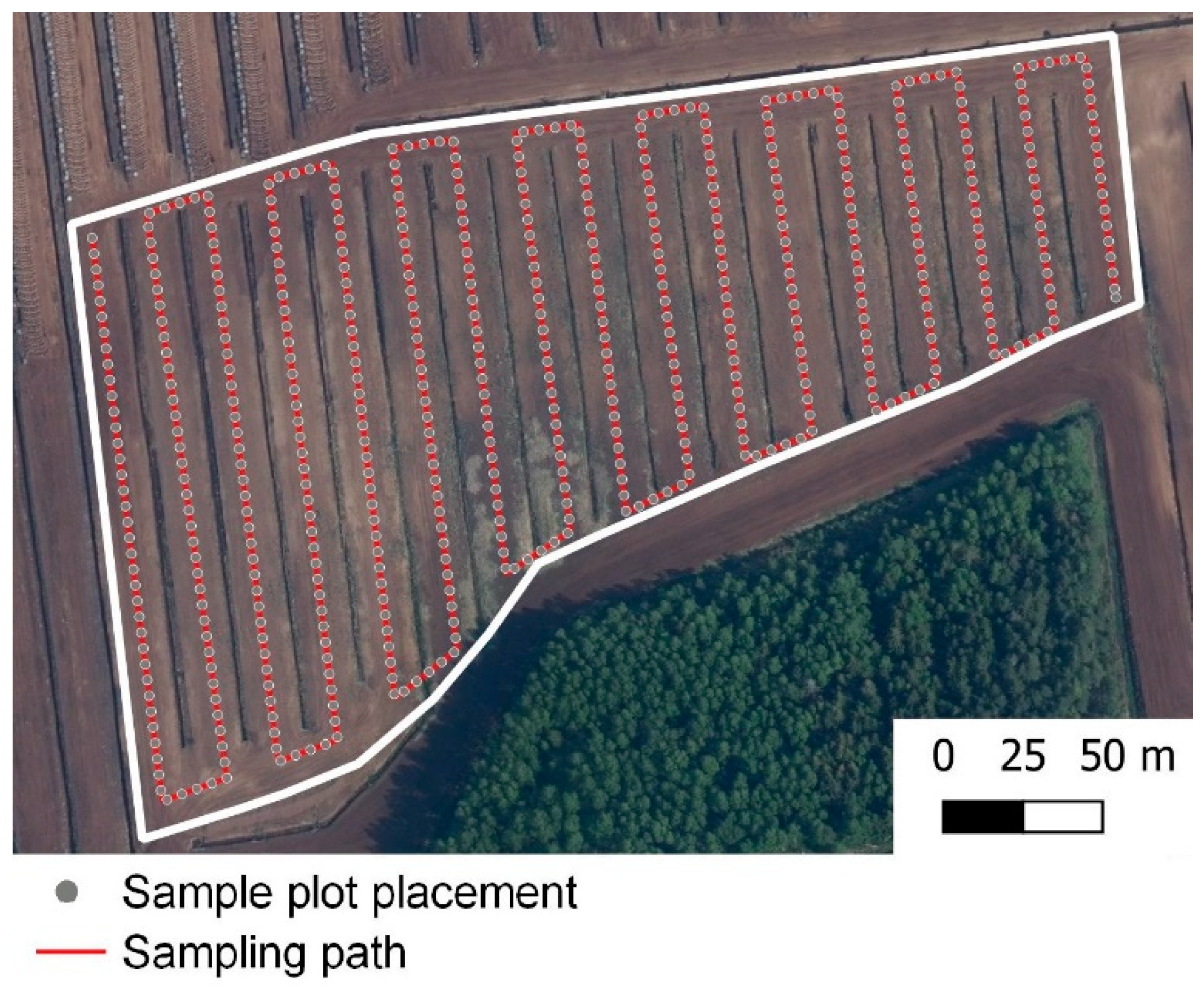
2.1. Research Sites

Data were collected from two sites, both of which are peat extraction locations. While peat extraction is ongoing in certain parts of these sites, other parts have been abandoned or restored. One of the two objects—the Raku mire—comprises three abandoned peat extraction fields and is located in the northern part of Latvia, Valmiera county. At this site, the terrain is fragmented and is considered hilly plainland with an average elevation of 85 m a.s.l. Annual precipitation according to climatic norm (State Limited Liability Company “Latvian Environment, Geology and Meteorology Centre”, Latvia, Riga, Maskavas iela 165) is 726 mm, which is higher than average in Latvia (680 mm). However, during our study period, conditions were drier with an average average annual precipitation of 715 mm. The average annual air temperature is 6.5 °C, but during our study it averaged 6.9 °C, which is slightly warmer. The second object—Kaigu mire—consists of eight fields, and is located in Jelgava County, central Latvia (Figure 1). The terrain in this area is flat, and can be described as lowland, with an average elevation of 3 m a.s.l. The average annual precipitation is 580 mm, which is lower than the national average and the average air temperature is 7.2 °C, which is slightly higher than the national average (6.8 °C). July is the rainiest month with an average precipitation of 77.1 mm, whereas March is the driest month, with an average precipitation of 29 mm. During our study period conditions were drier than the climatic norm, with an annual average precipitation of 490 mm. The average air temperature during the study period was 7.5 °C. The prevailing wind direction in both of sites is S—SW, and the average wind speed is between 3.2 and 3.5 m/s. The combined area of both sites is approximately 2000 ha. Our study concentrated on ground elevation changes and carbon losses in sections where peat extraction is currently terminated, encompassing roughly 96 ha.
Both of the study areas were drained more than 30 years ago and the initial depth of the peat layer before drainage was 5 m. Peat extraction in these sites was carried out using the cut block method; the remaining peat layer varied in size from 1 to 1.5 m. The groundwater table was measured in both study sites, but could not be attributed to the specific fields which were analyzed in this study. In Raku mire, the groundwater table fluctuates from 15 cm in December to 93 cm in July, but the mean level in the vegetation season is 66 cm. In Kaigu mire, it fluctuates from 28 cm in December to 100 cm in August, while the level in the mean vegetation season is 75 cm.
We used DJI Phantom 4 Multispectral UAV (DJI (Da-Jiang Innovations), Shenzhen, China) for multispectral data acquisition, and DJI Zenmuse L1 LiDAR mounted on a DJI Matrice 300 drone for LiDAR data acquisition. The estimated vertical accuracy for the LiDAR device is ±5 cm and the horizontal accuracy is 10 cm, and for Phantom 4 Multispectral drone, its positioning vertical positioning accuracy is 1.5 cm, but the horizontal accuracy is 1 cm. Data from all objects were acquired from June 2021 to May 2023, conducting flights monthly when the land is not covered by snow. For comparison, we used data from the Latvian Geospatial Information Agencies LiDAR (Latvian Geospatial Information Agency (LGIA), Latvia, Riga, Ojara Vaciesa iela 43) as a reference. The data for Kaigu mire were obtained on 30 September 2014, and for Rāķu mire on 4 September 2019. The estimated reference data accuracy is 1.34 and 1.27 cm, respectively. Our initial approach was to acquire data after strong wind periods, when possible, conducting monthly flights during the vegetation season. This approach was supplemented by additional, less frequent flights. Regular surveys, as shown in Table 1, were started in 8 fields (A, B, C, D, E, F, G, H), where full analysis was conducted. Starting from 27 July 2022, an additional 3 fields were added (I, J, K).
Using the obtained LiDAR data, digital elevation models (DEMs) with horizontal resolution of 20 cm were created from each survey, but using multispectral imagery, multispectral orthophoto maps in same 20 cm resolution were created.
In each field, ground control points (GCPs) were placed using the Trimble R8s system (Sunnyvale, CA, USA), and precise (RTK) location and elevation were measured for each survey. GCP data were used to georeference each survey in Agisoft Metashape Pro (Agisoft LLC, St. Petersburg, Russia).
To obtain ground elevation changes and dynamics of vegetation cover, expressed as the NDVI index, data were analyzed in virtual sample plots. In each study field path, which tends to be located between the ditches, sample plots with a 4 m diameter (12.56 m2) were placed at 5 m intervals (Figure 2). In each sample plot, the mean value and standard deviation of the elevation, Normalized Difference Elevation, Topographic Wetness index, and mean NDVI were calculated. The systematic arrangement of sample plots in fields offers several benefits for measuring ground elevation changes. It ensures representativeness by systematically covering the entire field and capturing spatial variability. The regular layout enables statistical analysis, facilitating trend detection, pattern identification, and spatial correlations.
Ground elevation change rates were calculated using QGIS 3.22.1 program raster calculator (r.mapcalc) and the data from each survey were then subtracted from the initial LGIA survey data. This method calculates the elevation change relative to the initial survey. This approach gives us the cumulative elevation change from the initial survey to each subsequent survey. It provides information about the overall subsidence and erosion caused elevation change trend over time. Each raster image is sampled using QGIS tool Zonal statistics.

2.2. Soil Analyses

Soil samples were collected in September 2022 using the equipment for undisturbed soil sampling (Eijkelkamp soil sampling ring kit C60, Nijverheidsstraat 30, 6987 EM, Giesbeek, The Netherlands). The volume of each sample was 100 cm3 and the sampling depth was 6 cm from the surface. Roots and large particles were avoided. Sampling was done avoiding the points marked with white in Figure 3, but not further than 5 m from the nearest measurement point. Sample density was estimated to acquire at least 1 peat sample per 10 measurement points.
After delivery to the laboratory samples were dried at 70 °C. After drying the samples were weighed to determine bulk density according to ISO 11272:2017 [40] standard and prepared for chemical analyses according to LVS ISO 11464:2005 L [41]. Then, C and nitrogen (N) content was determined using elemental analyzer Elemental EL Cube (Elementar Analysensysteme GmbH, Elementar-Straße 1, 63505 Langenselbold, Germany) according to LVS ISO 10694:2006 [41] and LVS ISO 13878:1998 [42] standards.
Results of soil analyses were interpolated across the study area using Heatmap (Kernel Density Estimation) function of QGIS application and specific values of C and N content were assigned to each measurement point using the Rasterize function of QGIS application.

2.3. Carbon Loss Estimation

We used the bulk density and the C amount of peat’s top layer to calculate soil C stock, using the mean values from each field. To estimate C loss due to subsidence, we used mean annual ground elevation change rates (cm y−1) and C stock. We assumed that more than 30 years after drainage and after more than 15 years of abandonment and vegetation formation, the effect of peat compaction is minimal or absent [20,25,43]. In this study, we calculate the mean annual elevation change rate (in centimeters per year) multiplied by the carbon (C) stock in the soil as a measure of carbon loss. This approach takes into account various factors combined, including erosion and subsidence.

2.4. Statistical Analysis

All statistical analyses were carried out using R 4.3.1 [44]. The Kruskal–Wallis rank sum test and pairwise comparisons using the Wilcoxon rank sum exact test were used to evaluate possible differences in the mean values of ground elevation change, carbon losses and environmental variables, including NDVI value and peat chemistry. Correlations between carbon losses and environmental variables were tested with Spearman’s ρ (R package ‘corrplot’), using a significance level of 0.01. (the function cor() from R package ‘ggpmisc’ was used to compute the significance levels for Spearman’s rank correlations).
Environmental variables such as temperature, precipitation, vegetation cover and general chemistry (X) were used to explain the variance of instantaneous ground elevation changes (Y) in partial least squares (PLS) regression—a useful multivariate method for dealing with variables which are linearly related to each other, as this method is robust against intercorrelations among X-variables. In PLS, X variables were ranked according to their relevance in explaining Y, commonly expressed as the Variable Importance in Projection (VIP values). In PLS regression, only X variables with VIP values exceeding 0.5 were included, and those with VIP values exceeding 1.0 were considered particularly important. R package ‘mdatools’ was used to compute the PLS regression. Data visualization was performed using GRASS GIS 8.2 and ArcMap 10.8 for spatial data and maps, but graphs were created using R package ‘ggplot2′.

3. Results

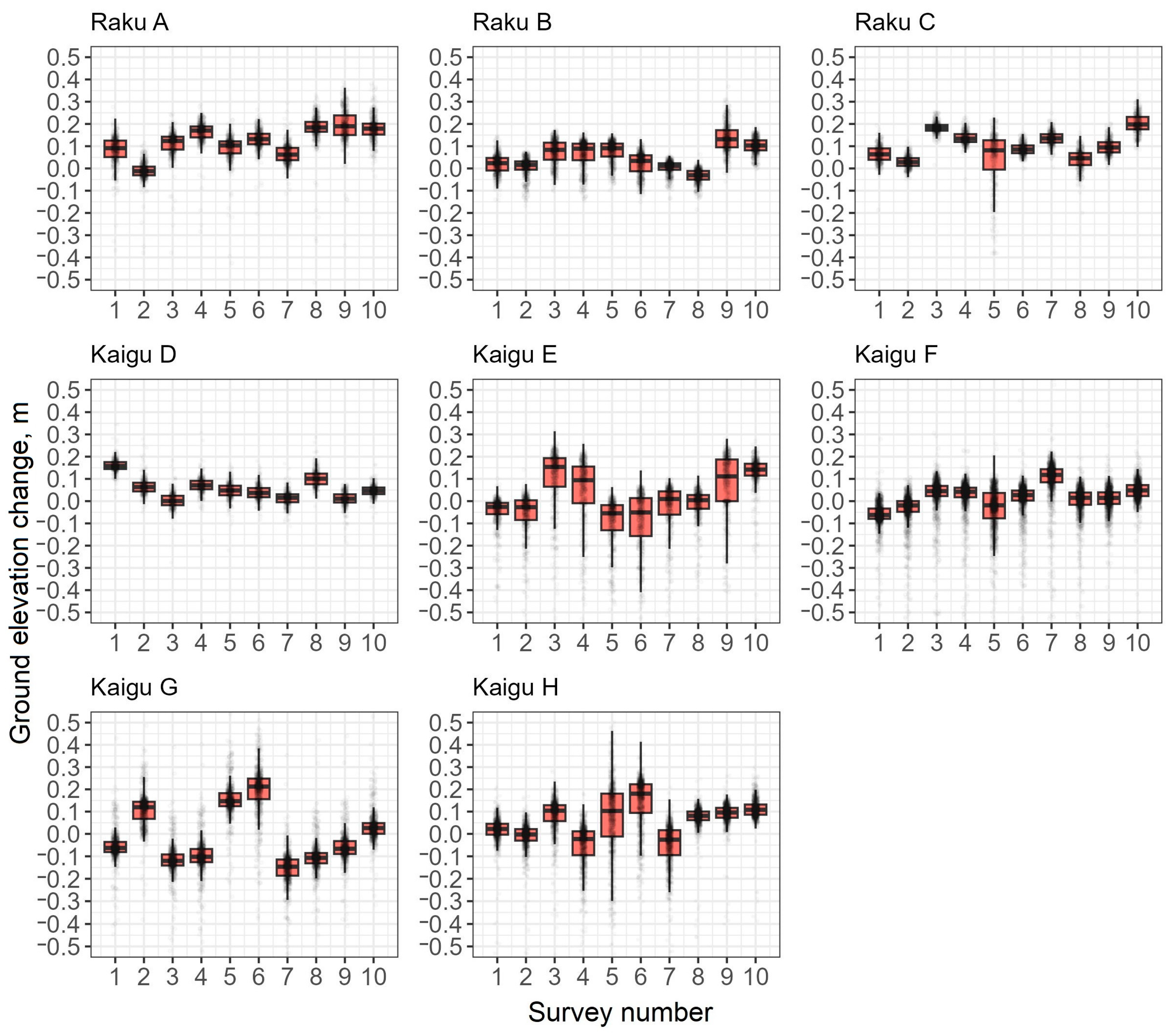
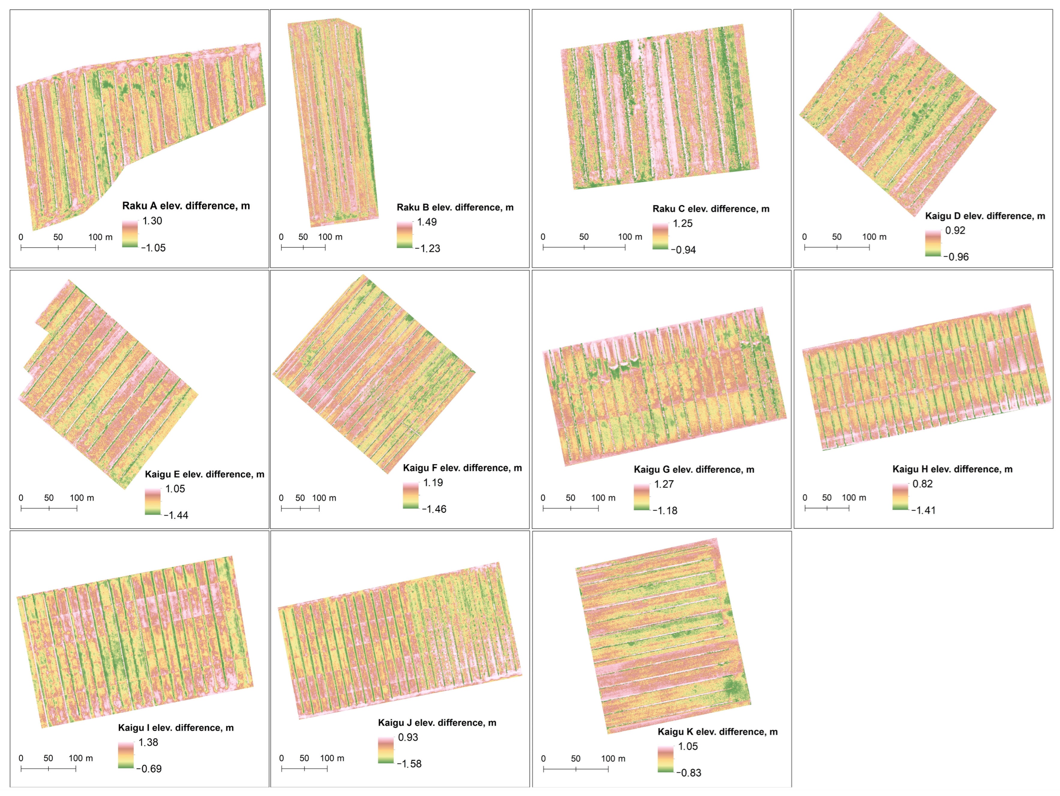
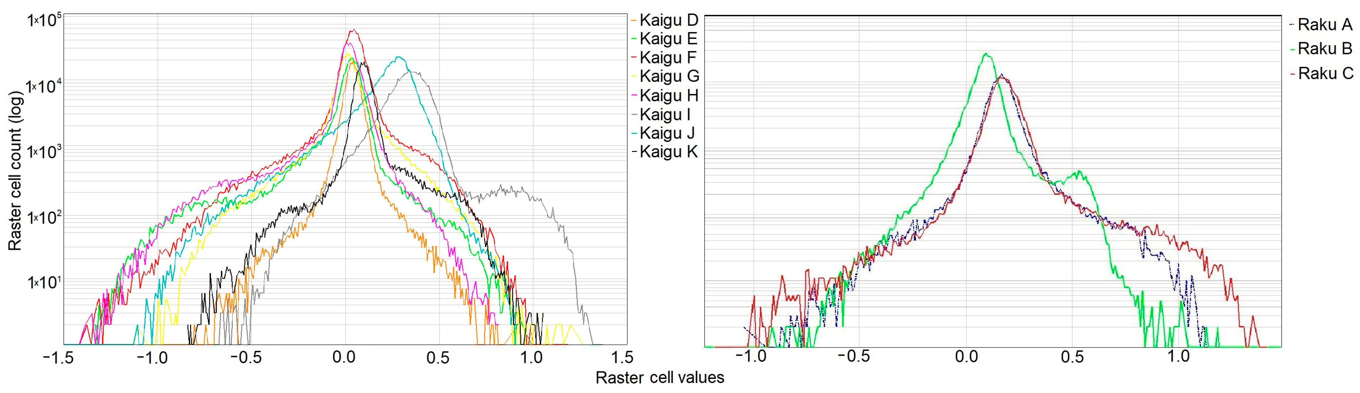
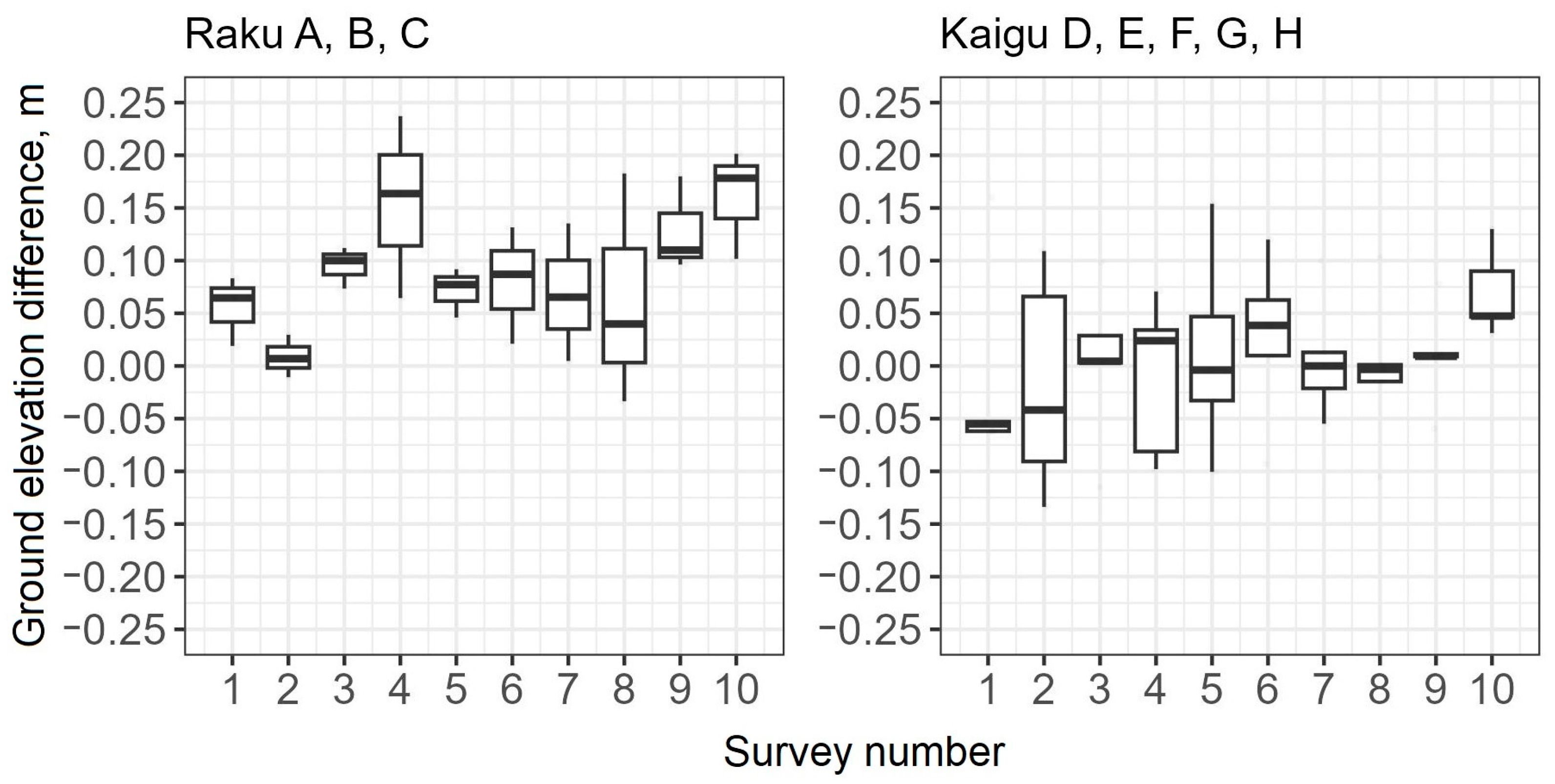
3.1. Evaluation of Ground Elevation Changes in Peatlands

The period between reference survey and surveys performed in the framework of our study differs between both study areas, Raku and Kaigu mires, as shown in Table 1. In Raku mire, the time between reference survey and Survey 1 is 631 days or 1.72 years, but in Kaigu mire time between reference survey and Survey 1 is 6.71 years.
Our results revealed high temporal and spatial variability in ground elevation changes at abandoned peat extraction sites. Patterns of ground elevation differences varied between the two study sites. Field in Raku mire showed more consistent trends within each survey (σ = 4.4 cm) compared to those observed in fields of Kaigu mire (σ = 6.7 cm) (Figure 3 and Figure 4).
In Raku A, Survey 1 showed ground elevation change (8.3 cm), followed by significant uplift in Survey 2 (1.0 cm). The subsequent surveys in Raku A revealed fluctuation in ground elevation, with varying degrees of elevation change. Raku B exhibited a mix of elevation decrease and uplift in different surveys, while Raku C in 2021 experienced a similar trend to Raku A. In Kaigu mire, Kaigu D showed elevation decrease in Survey 1 and relatively stable decrease in Surveys 2 to 10. Kaigu E demonstrated fluctuations in ground elevation between the surveys, with periods of uplift and decrease. Kaigu F showed an initial uplift in Surveys 1 and 2, followed by a relatively stable slight decrease in Surveys 3 to 10, except for Survey 7. Kaigu G and Kaigu H showed varying elevation changes with alternating uplift and decrease, with increasing decremental rates in the final surveys.
As shown in Figure 4, there are significant and spatially distributed ground elevation differences between the reference survey and Survey 10. We observed not only the overall field level ground elevation changes, but also peat surface movement. This movement can be associated with wind and water erosion, combined with vegetation cover. The results highlight the areas where peat movement has occurred.
The histogram of raster images, as shown in Figure 5, similarly to the previous image, indicates variations in height changes across the fields. When comparing the reference surveys with the last LiDAR scans, conducted on 10 May 2023, we found that the raster image statistics from the full field images in Raku mire study site compare well with the regular sample plot approach. In the Raku A field, the raster image indicates an elevation change of 17.8 ± 11.6 cm; in Raku B it is 10.4 ± 9.3 cm and in Raku C it is 19.2 ± 13.5 cm. However, higher uncertainty is observed in all three fields, when compared to sampling method. Raster statistics from Kaigu mire fields show a similar tendency in field level mean elevation change rates as observed with the sampling method. In comparison to the reference survey, the mean elevation difference values for Kaigu fields are as follows: Kaigu D shows a ground elevation change of 4.6 ± 16.6 cm; Kaigu E, 11.3 ± 11.2 cm; Kaigu F, 5.1 ± 13.2 cm; Kaigu G, 2.9 ± 14.2 cm; and Kaigu H, 10.8 ± 14.8 cm. In both Raku and Kaigu mire fields, there is a higher uncertainty when analyzing whole raster images, compared to the regular sampling method. Sample plots are mainly located between the ditches, whereas image analysis includes both field sides and ditches.
To estimate annual mean ground elevation changes, we used linear regression analysis, where ground elevation difference depends on time. The mean elevation difference value from each field and survey was used. The analysis was grouped by study sites—Kaigu and Raku mires, but regression was calculated for each field. Furthermore, we analyzed two time periods—from initial reference measurement and during our 10-survey research period. Regression analysis from Raku A shows an average annual elevation change of 5.72 cm (R2 = 0.60) over 3.6 years, but during our surveying period (1.75 years), there was an annual decrease of 7.0 cm (R2 = 0.49) (Figure 6). In fields Raku B and C there is a weak linear relationship and high variance in ground elevation differences. The mean annual decrease for Raku B is 2.1 cm (R2 = 0.17) over the full measurement period and 2.4 cm (R2 = 0.1) over past 1.75 years, but Raku C the annual decrease are 4.4 cm (R2 = 0.3) and 4.3 cm (R2 = 0.14), respectively.
For Kaigu mire fields during full measurement period of 8.6 years, no linear relationship between time and ground elevation differences is detected, and the vertical land motion is determined by other factors. However, during our surveying period (1.9 years) a weak correlation in fields Kaigu E, F and H is evident, where the annual ground decremental rates are 8.7 cm (R2 = 0.33), 4.0 cm (R2 = 0.27) and 4.4 cm (R2 = 0.29), respectively.

3.2. Evaluation of Carbon Losses Due to Subsidence and Erosion

The results, also shown in Table 2, reveal notable variability in soil density among the abandoned peat extraction sites. Raku C demonstrated the highest mean soil density of 159.40 ± 52.86 g cm−3, while Kaigu D exhibited the lowest mean soil density of 73.38 ± 6.24 g cm−3. Standard deviation values were used to quantify the uncertainty in the soil density measurements. Raku C had the highest standard deviation, indicating significant variability in soil density within that location. Conversely, Kaigu D showed the lowest standard deviation, suggesting relatively consistent measurements.
Among the sites, Kaigu H exhibited the highest mean total carbon concentration of 539.93 ± 19.62 g kg−1, while Site 3 showed the lowest mean total carbon concentration of 444.95 ± 107.86 g kg−1. Kaigu D, E, F, and G had similar mean carbon concentrations in the range of 505.92 to 516.81 g kg−1. The standard deviation values provide information about the spread of data points around the mean value. Raku C and Kaigu H had the highest standard deviations, indicating more variability and uncertainty in carbon content within these sites. In contrast, Kaigu J had the lowest standard deviation of 10.22 g kg−1.
The average total nitrogen concentration in peat was found to vary among the sites, ranging from 7.93 ± 1.84 to 13.71 g kg. Raku B displayed the highest mean total nitrogen concentration, with a value of 13.71 ± 2.56 g kg, while Kaigu G had the lowest mean concentration of 7.93 g kg. Raku A and Kaigu H showed the highest standard deviations, indicating more variability in total nitrogen concentration within these sites. In contrast, Kaigu I had the lowest standard deviation.
There is significant variability in total carbon stock in our study sites, with values ranging from 37.14 ±3.50 kg m3 to 76.17 ± 14.85 kg m3. Kaigu H has the highest mean carbon amount, registering 76.17 kg m3, whereas Kaigu D displayed the lowest mean carbon stock at 37.14 ± 3.50 kg m3.
Raku B and Kaigu H had the highest standard deviations, indicating greater variability in carbon stock within these sites. Conversely, Kaigu G demonstrated the lowest standard deviation.
Carbon losses are estimated using mean annual field-level ground elevation change rates. Decreased ground elevation is converted as m3/m2 peat subsidence and erosion and using carbon content measures, also shown in Table 3, carbon losses are calculated.
Annual carbon losses vary from 0.05 ± 5.33 kg m−2 y−1 in Kaigu G, where also high ground elevation change uncertainty is observed (0.1 ± 8.2 cm y−1), to 3.57 ± 4.06 kg m−2 y−1 in Raku A. We can assume, that highest ground elevation decreases and C loss rates are observed in Raku mire fields, where annual mean elevation decrease varies between fields from 2.14 ± 5.7 cm y−1 in Raku B, to 5.72 ± 5.4 cm y−1 in Raku A, but C loss—from 1.21 ± 5.12 kg m−2 y−1 in B to 3.57 ± 4.06 kg m−2 y−1 in Raku A.
Fields in Kaigu mire show high fluctuations in ground elevation and high uncertainty, respectively. In each Kaigu mire field, annual mean ground elevation decrease is less than 1 cm, ranging from 0.08 ± 8.3 cm y−1 in Kaigu H to 0.58 ± 3.5 cm y−1 in Kaigu D. Annual mean C loss can be estimated as 0.05 ± 5.33 kg m−2 y−1 in Kaigu G to 0.22 ± 1.63 kg m2 y−1 in Kaigu D.

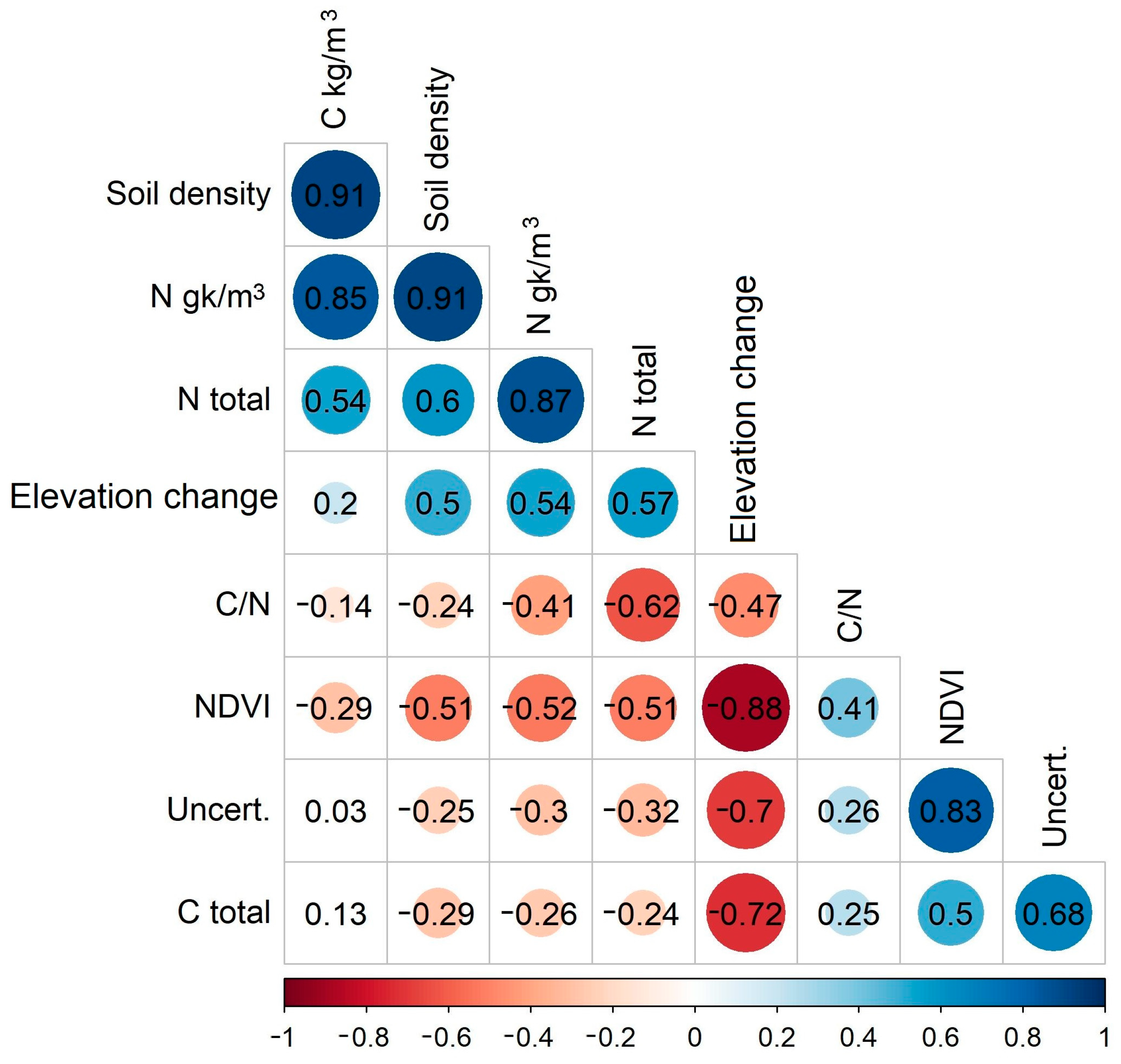
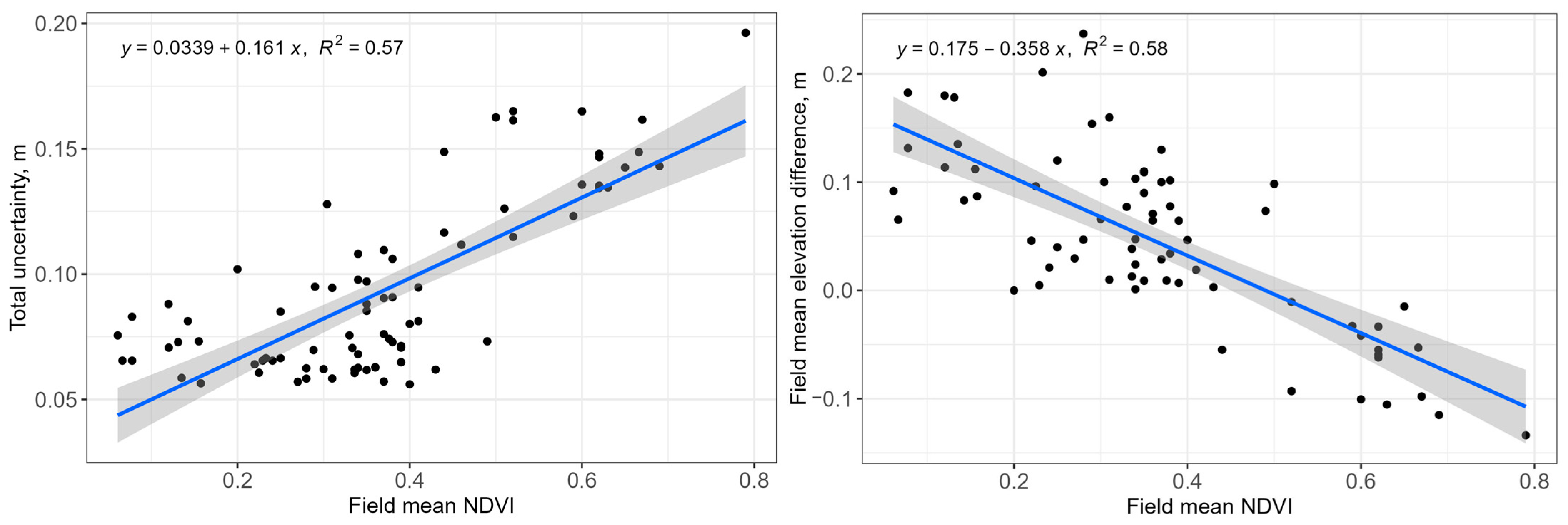
3.3. Evaluation of Affecting Factors and Total Carbon Losses

Ground elevation changes in abandoned peat extraction sites had a strong negative correlation with NDVI value (r = −0.88, p < 0.001), total uncertainty (p < 0.001) and total C stock in peat (p < 0.001) (Figure 7). There was also a significant negative relationship with C/N (r = −0.47, p = 0.004) and positive correlations with N in peat (r = 0.57, p = 0.01) and soil density (r = 0.5, p = 0.002). Additionally, there were strong correlation between NDVI and total uncertainty in results (r = 0.83, p < 0.001) and NDVI with nitrogen in peat (r = 0.51, p = 0.01). All these factors have a strong effect on ground elevation differences.
Linear regression analysis (Figure 8) revealed a significant linear relationship between the field mean NDVI value and the field mean elevation difference (R2 = 0.58). The Field mean NDVI value was also identified as a significant factor affecting the total uncertainty in mean field-level ground elevation differences (R2 = 0.57). The impact of NDVI on ground elevation difference strongly increases when field mean NDVI value exceeds 0.4. A PLS model revealed that ground elevation decrease can be partly explained with NDVI and C/N (R2 = 0.52). Nevertheless, we did not find any significant relationships between ground elevation changes and meteorological variables, such as air temperature, precipitation, and strong wind events, in our research period.

4. Discussion

4.1. Ground Elevation Changes

Within each field and study site we observed highly fluctuating ground elevation differences (Figure 9). The mean annual ground elevation decrease rates ranged from 0.08 ± 8.3 cm y−1 to 0.58 ± 3.5 cm y−1 in Kaigu mire, and 2.14 ± 5.7 cm y−1 to 5.72 ± 5.4 cm y−1 in Raku mire. In older study, conducted in Canada [45], where erosion of Histosol in agricultural land was monitored over the long term, alternating elevation change rates were observed, ranging from 0.99 ± 1.59 cm y−1 in protected fields to 4.53 ± 2.29 cm y−1 in fields without conservation measures.
Many studies from temperate Europe have evaluated erosion and subsidence in different types of peatlands [24,28,29,34,35,46,47]. These studies report annual mean subsidence rates from 0.27 cm y−1 to 2.8 cm y−1, mostly less than 1 cm y−1. The elevation changes associated with subsidence rates depend on the type of peatland management, with the highest annual rates observed in cultivated peatlands. In an older study, conducted in Canada [45] where erosion of Histosol in agricultural land was monitored in the long term. In this study alternating subsidence rates ranging from 0.99 ± 1.59 cm y−1 in protected fields to 4.53 ± 2.29 cm y−1 in fields with no conservation measures were observed. Our research aligns more closely with studies conducted in hemiboreal and boreal climate zones [18,27,48], where elevation decrease varies from 0.5 cm y−1 to 2.8 cm y−1. While our annual elevation decrease estimates are largely in line with the results of these studies, in some fields, for example Raku B and Raku A, decrease is considerably higher (4.4 ± 3.4 cm y−1 to 5.72 ± 5.4 cm y−1). These elevation change rates linked to subsidence and erosion are similar to those reported in tropical regions [20,49,50], where subsidence rates reached up to 5 cm y−1. Nevertheless, our findings demonstrate that significant rates of subsidence and erosion can occur even in cooler climatic conditions over prolonged periods. In hemiboreal latitudes, while biochemical mechanisms may slow down for most of the year, they still lead to considerable degradation throughout the growing season. There is an undeniable effect of drainage-induced moisture changes on peat mineralization and subsidence [20,25]. Factors such as drainage intensity, time after drainage and, to some extent, distance between drainage ditches are proved to be important subsidence drivers. In our study, we do not evaluate these factors. We also did not assess the groundwater level, which has an impact on vertical land movement, specifically, lower levels lead to higher subsidence [20,24,50].
Using remote sensing data, we observed that in most of our study areas ground elevation change is dependent on NDVI value (R2 = 0.58), suggesting that higher prevalence of vegetation in the field likely prevents ground subsidence and erosion. In both fields (Raku A and C), where the highest elevation decrease rates were observed, the mean NDVI values were the lowest (0.21 ± 0.09 and 0.25 ± 0.11, respectively), which corresponds to higher area ratio with bare peat. Simultaneously, in Kaigu mire fields, where ground elevation differences showed high uncertainty and were significantly lower than in Raku mire fields, the mean NDVI values were higher, ranging from 0.34 ± 0.04 in Kaigu D to 0.54 ± 0.13 in Kaigu E. We found a relationship between NDVI and subsidence rates in field-level values, but the correlation was weak at the sample plot level. Vegetation cover protects and delays bare peat surface from weathering [2,51,52]. Zhongming et al. [53] also highlights the importance of vegetation cover in preventing soil erosion—the degree of erosion varies not only by the presence of vegetation, but also by variations in its type and structure.
Most studies, primarily conducted in the UK and focused on gully erosion in blanket bogs, have concluded that erosion is mainly driven by surface water flow on gully walls and bottom. The erosion mostly occurs after heavy rain events. These studies have validated the use of remote sensing techniques, such as ALS, TLS, and SfM photogrammetry, for detecting water erosion in peatland gullies [31,33,34,35]. On the other hand, our study provides multi-temporal ALS data-based elevation change detection. However, our methods do not allow us to separate individual factors, such as erosion or mineralization, from cumulative ground elevation decremental rates (Figure 9).
Water erosion in ditches and ditch walls have been extensively studied [9,54,55]. It has been found that in peat extraction sites erosion mostly occurs from ditches and ditch walls during rainfall events. Our results (Figure 4) partly align with this observation. In certain cases, we observed significant erosion from ditch sides deposition in ditch beds, as well as peat deposition on ditch sides due to vegetation presence, which hold back erodible peat.

4.2. Carbon Losses

Our results show that Raku mire has the highest mean peat density, ranging from 119.85 ± 42.78 kg m−3 in B field, to 159.40 ± 52.86 kg m−3 in C field. The peat density in Kaigu mire varies from 73.38 ± 6.24 kg m−3 in D field to 140.28 ± 23.47 kg m−3 in H field. These results align with previously published peat surface (up to 10 cm) bulk density values in Latvia [48]. However, our values are lower than those measured in Finland and Norway [27,56]. These differences can be explained by the time since peatland drainage and the respective compaction rates. Nevertheless, at Raku mire we observed the lowest C content in peat upper layer ranging from 444.95 ± 107.86 g kg−1 in C field, to 496 ± 89.26 g kg−1 in A field, while in Kaigu mire C content ranges from 505.96 ± 13.00 g kg−1 to 539.93 ± 19.62 g kg−1, which is similar carbon content rate in peat as reported in other studies [32,35,50].
We estimated annual peat loss rates due to subsidence and erosion in both Kaigu and Raku mire fields with high uncertainty. In Kaigu mire, the rates range from 0.001 ± 0.083 m3 m−2 y−1 to 0.006 ± 0.035 m3 m−2 y−1 and for Raku mire fields, the rates are between 0.021 ± 0.057 m3 m−2 y−1 and 0.057 ± 0.054 m3 m−2 y−1. Accordingly, mean annual carbon losses range from 0.05 ± 5.33 kg m−2 y−1 to 0.22 ± 1.63 kg m−2 y−1 in Kaigu mire and from 1.21 ± 5.12 kg m−2 y−1 to 3.57 kg m−2 y−1 in Raku mire. Significant variability between Kaigu and Raku mires is determined by varied subsidence and erosion rates, which are closely related to vegetation cover, as described by NDVI. Subsidence rates of 0.8–1.6 cm y−1 have been reported in a study from Switzerland (Leifeld et al. 2011), which corresponds to an annual carbon loss ranging from 0.25 to 0.55 kg m−2 y−1. Annual carbon loss rates from 0.80 kg m−2 y−1 to 0.86 kg m−2 y−1 are estimated in study from Norway [27]. Our results are mostly within these estimates, except from Raku mire fields, where we estimated higher elevation decrease and carbon loss. In SE Asia peatland plantations fields, carbon loss can also be as high as 2.7–3.0 kg m−2 y−1 [50]. Wösten et al., 1997 and Ansahri et al., 2021 [19,49] used oxidized subsidence factor 0.6 to calculate C loss from each subsided peat cm, using assumption that 60% of subsidence is peat mineralization but 40% is compaction. In these studies, variations in carbon loss values within the observed range can be partly attributed to disparities in water table depth. However, factors such as vegetation cover and the introduction of fertilizers also play a role in affecting peat oxidation. The connection with groundwater table depth underscores that significant levels of subsidence and carbon loss persist. Additionally, factors such as peat layer depth, compaction and time after drainage have an important role in peat subsidence. These factors were not analyzed in our study. However, in the study conducted in German temperate bog [57], they found that together with peat oxidation induced by drainage, also C:N ratio of the peat layer is declining from the actively degrading topsoil layers to the underlying, less decomposed peat, which is also associated by an increase in soil bulk density. These findings can be attributed to the results observed in our study, as we found positive correlation with elevation changes and nitrogen content, as well as negative correlation with C:N ratio and elevation changes.

5. Conclusions

Our results show that peatland elevation change rates vary significantly not only seasonally, but also over short intervals, such as weeks. By using time series of ground elevation differences and NDVI data, regression analysis allowed us to estimate mean annual elevation decrease rates. Notably, these rates can vary more than tenfold between the two study sites. We found that uncertainty in elevation differences and field-level mean subsidence and erosion can be partly explained by NDVI value, which represents vegetation cover. The PLS model revealed that elevation changes linked to subsidence and erosion can be partly explained by NDVI and the C:N ratio.
Estimated elevation decrease and resulting carbon losses also vary significantly between field and both study sites, but mostly are within range of results presented in other studies conducted in boreal, as well as temperate climate zones. There was high uncertainty in our results which can be reduced slightly by continuing ground elevation data acquisition to obtain more long-term high-resolution elevation data. Nevertheless, uncertainty still can be very high, mostly due to the mire breathing process, which we observed, and high spatial differences of ground elevation, due to peat movement driven by wind and other environmental factors.
Our study reveals that ground elevation changes in peatlands should be studied over the long term, as very high fluctuations were observed during our study period. Spatial differences in elevation changes, accompanied by high fluctuations overall, and correlation with the C:N ratio indicate that ground elevation change in peatlands is driven by various factors, including erosion, oxidation, and subsidence. However, to gain a deeper understanding of these processes, additional consistent surveys as well as long-term data on aspects such as peat layer depth, peat composition, and groundwater level should be obtained. However, carbon losses from peat extraction sites should be studied extensively and the results evaluated with caution, for better understanding, if this carbon should be accounted as input in other areas, as well as it may overlap with reported dissolved organic carbon; therefore, the reporting of carbon losses due to peat subsidence and erosion should be considered carefully to avoid double accounting of emissions in the national GHG inventories.

Author Contributions

Conceptualization, R.N.M.; methodology, A.L.; software, J.C. and R.N.M.; validation, A.B. (Arta Bārdule), I.S. and A.L.; formal analysis, R.N.M.; investigation, R.N.M., S.K. and A.B. (Aldis Butlers); resources, A.L.; data curation, A.L.; writing—original draft preparation, R.N.M., G.P. and S.K.; writing—review and editing, A.B. (Aldis Butlers) and G.P.; visualization, A.B. (Arta Bārdule) and R.N.M.; supervision, A.L.; project administration, A.L.; funding acquisition, A.L. All authors have read and agreed to the published version of the manuscript.

Funding

This research was funded by European Regional Development Fund project “Development of greenhouse gas emission factors and decision support tools for management of peatlands after peat extraction”, grant number 1.1.1.1/19/A/064. R.M. contribution was supported by doctoral grant project (No. 8.2.2.0/20/I/006), A.L., G.P., A.Bā., A.Bu., S.K. and I.S. contribution was supported by European Regional Development Fund project “Evaluation of factors affecting greenhouse gas (GHG) emissions reduction potential in cropland and grassland with organic soils” (1.1.1.1/21/A/031). J.C. contribution was supported by EU LIFE Programme project “Demonstration of climate change mitigation potential of nutrient rich organic soils in Baltic States and Finland” (LIFE OrgBalt, LIFE18 CCM/LV/001158).

Data Availability Statement

The data presented in this study are available on request from the corresponding author, Raitis Melniks. The data are not publicly available due to private interests of the research site owners.

Conflicts of Interest

The authors declare no conflict of interest. The funders had no role in the design of the study; in the collection, analyses, or interpretation of data; in the writing of the manuscript; or in the decision to publish the results.

References

  1. Joosten, H. Peatlands across the Globe. In Peatland Restoration and Ecosystem Services: Science, Policy and Practice; Bonn, A., Allott, T., Evans, M., Joosten, H., Stoneman, R., Eds.; Cambridge University Press: Cambridge, UK, 2016; pp. 19–43. [Google Scholar]
  2. Li, C.; Grayson, R.; Holden, J.; Li, P. Erosion in peatlands: Recent research progress and future directions. Earth-Sci. Rev. 2018, 185, 870–886. [Google Scholar] [CrossRef]
  3. Hilbert, D.W.; Roulet, N.; Moore, T. Modelling and analysis of peatlands as dynamical systems. J. Ecol. 2000, 88, 230–242. [Google Scholar] [CrossRef]
  4. Frolking, S.; Talbot, J.; Jones, M.C.; Treat, C.C.; Kauffman, J.B.; Tuittila, E.-S.; Roulet, N. Peatlands in the Earth’s 21st century climate system. Environ. Rev. 2011, 19, 371–396. [Google Scholar] [CrossRef]
  5. Xu, J.; Morris, P.J.; Liu, J.; Holden, J. PEATMAP: Refining estimates of global peatland distribution based on a meta-analysis. Catena 2018, 160, 134–140. [Google Scholar] [CrossRef]
  6. McNeil, P.; Waddington, J.M.; Lavoie, C.; Price, J.S.; Rochefort, L. Contemporary and long-term peat oxidation rates in a post-vacuum harvested peatland. In Sustaining Our Peatlands, Proceedings of the 11th International Peat Congress, Edmonton, AB, Canada, 6–12 August 2000; Rochefort, L., Daigle, J.Y., Eds.; Canadian Society of Peat and Peatlands & International Peat Society: Quebec city, QC, Canada, 2000; Volume 2, pp. 732–741. [Google Scholar]
  7. Campbell, D.R.; Lavoie, C.; Rochefort, L. Wind erosion and surface stability in abandoned milled peatlands. Can. J. Soil Sci. 2002, 82, 85–95. [Google Scholar] [CrossRef]
  8. Littlewood, N.; Anderson, P.; Artz, R. Peatland Biodiversity. Report to IUCN UK Peatland Programme, Edinburgh. Available online: www.iucn-uk-peatlandprogramme.org/scientificreviews (accessed on 14 September 2023).
  9. Kløve, B. Erosion and sediment delivery from peat mines. Soil Tillage Res. 1998, 45, 199–216. [Google Scholar] [CrossRef]
  10. Evans, M.; Lindsay, J. High resolution quantification of gully erosion in upland peatlands at the landscape scale. Earth Surf. Process Landf. 2010, 35, 876–886. [Google Scholar] [CrossRef]
  11. Evans, M.; Lindsay, J. Impact of gully erosion on carbon sequestration in blanket peatlands. Clim. Res. 2010, 45, 31–41. [Google Scholar] [CrossRef]
  12. Li, C.; Holden, J.; Grayson, R. Effects of rainfall, overland flow and their interactions on peatland interrill erosion processes. Earth Surf. Process Landf. 2018, 43, 1451–1464. [Google Scholar] [CrossRef]
  13. McLay, C.D.A.; Allbrook, R.F.; Thompson, K. Effects of development and cultivation on physical properties of peat soils in New Zealand. Geoderma 1992, 54, 23–37. [Google Scholar] [CrossRef]
  14. Price, J.S.; Schlotzhauer, S.M. Importance of shrinkage and compression in determining water storage changes in peat: The case of a mined peatland. Hydrol. Proc. 1999, 13, 2591–2601. [Google Scholar] [CrossRef]
  15. Holden, J.; Chapman, P.J.; Labadz., J.C. Artificial drainage of peatlands: Hydrological and hydrochemical process and wetland restoration Progress in Physical Geography. Earth Environ. 2004, 28, 95–123. [Google Scholar]
  16. Van Hardeveld, H.A.; Driessen, P.P.J.; Schot, P.P.; Wassen, M.J. an integrated modelling framework to assess long-term impacts of water management strategies steering soil subsidence in peatlands. Environ. Impact Assess. Rev. 2017, 66, 66–77. [Google Scholar] [CrossRef]
  17. Leifeld, J.; Menichetti, L. The underappreciated potential of peatlands in global climate change mitigation strategies. Nat. Commun. 2018, 9, 1071. [Google Scholar] [CrossRef]
  18. Ikkala, L.; Ronkanen, A.-K.; Utriainen, O.; Kløve, B.; Marttila, H. Peatland subsidence enhances cultivated lowland flood risk. Soil Tillage Res. 2021, 212, 105078. [Google Scholar] [CrossRef]
  19. Wösten, J.H.M.; Ismail, A.B.; Van Wijk, A.L.M. Peat subsidence and its practical implications: A case study in Malaysia. Geoderma 1997, 78, 25–36. [Google Scholar] [CrossRef]
  20. Evans, C.D.; Williamson, J.M.; Kacaribu, F.; Irawan, D.; Suardiwerianto, Y.; Hidayat, M.F.; Laurén, A.; Page, S.E. Rates and spatial variability of peat subsidence in Acacia plantation and forest landscapes in Sumatra, Indonesia. Geoderma 2019, 338, 410–421. [Google Scholar] [CrossRef]
  21. van Asselen, S.; Erkens, G.; and de Graaf, F. Monitoring shallow subsidence in cultivated peatlands. Proc. IAHS 2020, 382, 189–194. [Google Scholar] [CrossRef]
  22. Davidson, E.; Janssens, I. Temperature sensitivity of soil carbon decomposition and feedbacks to climate change. Nature 2006, 440, 165–173. [Google Scholar] [CrossRef]
  23. Elder, J.W.; Lal, R. Tillage effects on physical properties of agricultural organic soils of north central Ohio. Soil Tillage Res. 2008, 98, 208–210. [Google Scholar] [CrossRef]
  24. Dawson, Q.; Kechavarzi, C.; Leeds-Harrison, P.; Burton, R.G.O. Subsidence and degradation of agricultural peatlands in the Fenlands of Norfolk, UK. Geoderma 2010, 154, 181–187. [Google Scholar] [CrossRef]
  25. Grzywna, A. The degree of peatland subsidence resulting from drainage of land. Environ. Earth Sci. 2017, 76, 559. [Google Scholar] [CrossRef]
  26. Maijala, T. About Subsidence of Relictions. In Viljeltyjen Vesijättöjen Painumisesta; National Board of Waters and the Environment: Helsinki, Finland, 1992. [Google Scholar]
  27. Grönlund, A.; Hauge, A.; Hovde, A.; Rasse, D.P. Carbon loss estimates from cultivated peat soils in Norway: A comparison of three methods. Nutr. Cycl. Agroecosyst. 2008, 81, 157–167. [Google Scholar] [CrossRef]
  28. Leifeld, J.; Müller, M.; Fuhrer, J. Peatland subsidence and carbon loss from drained temperate fens. Soil Use Manag. 2011, 27, 170–176. [Google Scholar] [CrossRef]
  29. Oleszczuk, R.; Zając, E.; Urbański, J. Verification of empirical equations describing subsidence rate of peatland in Central Poland. Wetlands Ecol. Manag. 2020, 28, 495–507. [Google Scholar] [CrossRef]
  30. Jeziorska, J. UAS for Wetland Mapping and Hydrological Modeling. Remote Sens. 2019, 11, 1997. [Google Scholar] [CrossRef]
  31. Evans, M.; Warburton, J. The Geomorphology of Upland Peat: Erosion, Form and Landscape Change; Wiley-Blackwell: Oxford, UK, 2007. [Google Scholar]
  32. Scholefield, P.; Morton, D.; McShane, G.; Carrasco, L.; Whitfield, M.G.; Rowland, C.; Rose, R.; Wood, C.; Tebbs, E.; Dodd, B.; et al. Estimating habitat extent and carbon loss from an eroded northern blanket bog using UAV derived imagery and topography. Prog. Phys. Geogr. 2019, 43, 282–298. [Google Scholar] [CrossRef]
  33. Evans, M.; Warburton, J.; Yang, J. Eroding blanket peat catchments: Global and local implications of upland organic sediment budgets. Geomorphology 2006, 79, 45–57. [Google Scholar] [CrossRef]
  34. Glendell, M.; McShane, G.; Farrow, L.; James, M.R.; Quinton, J.; Anderson, K.; Brazier, R.E. Testing the utility of structure-from-motion photogrammetry reconstructions using small unmanned aerial vehicles and ground photography to estimate the extent of upland soil erosion. Earth Surf. Process Landf. 2017, 42, 1860–1871. [Google Scholar] [CrossRef]
  35. Grayson, R.; Holden, J.; Jones, R.R.; Carle, J.A.; Lloyd, A.R. Improving particulate carbon loss estimates in eroding peatlands through the use of terrestrial laser scanning. Geomorphology 2012, 179, 240–248. [Google Scholar] [CrossRef]
  36. Rothwell, J.J.; Lindsay, J.B.; Evans, M.G.; Allott, T.E.H. Modelling suspended sediment lead concentrations in contaminated peatland catchments using digital terrain analysis. Ecol. Eng. 2010, 36, 623–630. [Google Scholar] [CrossRef]
  37. Simpson, J.; Wooster, M.; Smith, T.; Trivedi, M.; Vernimmen, R.; Dedi, R.; Shakti, M.; Dinata, Y. Tropical Peatland Burn Depth and Combustion Heterogeneity Assessed Using UAV Photogrammetry and Airborne LiDAR. Remote Sens. 2016, 8, 1000. [Google Scholar] [CrossRef]
  38. Ikkala, L.; Ronkanen, A.-K.; Ilmonen, J.; Similä, M.; Rehell, S.; Kumpula, T.; Päkkilä, L.; Klöve, B.; Marttila, H. Unmanned Aircraft System (UAS) Structure-From-Motion (SfM) for Monitoring the Changed Flow Paths and Wetness in Minerotrophic Peatland Restoration. Remote Sens. 2022, 14, 3169. [Google Scholar] [CrossRef]
  39. Kalacska, M.; Arroyo-Mora, J.P.; Lucanus, O. Comparing UAS LiDAR and Structure-from-Motion Photogrammetry for peatland mapping and virtual reality (VR) visualization. Drones 2021, 5, 36. [Google Scholar] [CrossRef]
  40. ISO 11272:2017; Soil Quality—Determination of Dry Bulk Density. International Organization for Standardization: Geneva, Switzerland, 2017.
  41. ISO 11464:2006; Soil Quality—Pretreatment of Samples for Physico-Chemical Analysis. International Organization for Standardization: Geneva, Switzerland, 2006.
  42. ISO 13878:1998; Soil Quality—Determination of Total Nitrogen Content by Dry Combustion (“Elemental Analysis”). International Organization for Standardization: Geneva, Switzerland, 1998.
  43. Sloan, T.; Payne, R.J.; Anderson, R.; Gilbert, P.; Mauquoy, D.; Newton, A.; Andersen, R. Ground surface subsidence in an afforested peatland fifty years after drainage and planting. Mires Peat 2019, 23, 1–12. [Google Scholar]
  44. R Core Team. R: A Language and Environment for Statistical Computing; R Foundation for Statistical Computing: Vienna, Austria, 2023; Available online: https://www.R-project.org/ (accessed on 14 September 2023).
  45. Parent, L.E.; Millette, J.A.; Mehuys, G.R. Subsidence and Erosion of a Histosoil. Soil Sci. Soc. Am. J. 1982, 46, 404. [Google Scholar] [CrossRef]
  46. Regan, S.; Flynn, R.; Gill, L.; Naughton, O.; Johnston, P. Impacts of groundwater drainage on peatland subsidence and its ecological implications on an Atlantic raised bog. Water Re. Res. 2019, 55, 6153–6168. [Google Scholar] [CrossRef]
  47. Fell, H.; Roßkopf, N.; Bauriegel, A.; Zeitz, J. Estimating vulnerability of agriculturally used peatlands in north-east Germany to carbon loss based on multi-temporal subsidence data analysis. Catena 2016, 137, 61–69. [Google Scholar] [CrossRef]
  48. Lupikis, A.; Lazdins, A. Soil carbon stock changes in transitional mire drained for forestry in Latvia: A case study. In Proceedings of the Research for Rural Development 2017: Annual 23rd International Scientific Conference Proceedings, Latvia, Jelgava, 17–19 May 2017; Latvia University of Agriculture: Jelgava, Latvia, 2017; Volume 1, pp. 55–61. [Google Scholar]
  49. Anshari, G.Z.; Gusmayanti, E.; Novita, N. The Use of Subsidence to Estimate Carbon Loss from Deforested and Drained Tropical Peatlands in Indonesia. Forests 2021, 12, 732. [Google Scholar] [CrossRef]
  50. Hooijer, A.; Page, S.; Jauhiainen, J.; Lee, W.A.; Lu, X.X.; Idris, A.; Anshari, G. Subsidence and carbon loss in drained tropical peatlands. Biogeosciences 2012, 9, 1053–1071. [Google Scholar] [CrossRef]
  51. Harris, A.; Baird, A.J. Microtopographic drivers of vegetation patterning in blanket peatlands recovering from erosion. Ecosystems 2019, 22, 1035–1054. [Google Scholar] [CrossRef]
  52. Shuttleworth, E.L.; Evans, M.G.; Hutchinson, S.M.; Rothwell, J.J. Peatland restoration: Controls on sediment production and reductions in carbon and pollutant export. Earth Surf. Process Landf. 2000, 40, 459–472. [Google Scholar] [CrossRef]
  53. Zhongming, W.; Lees, B.G.; Feng, J.; Wanning, L.; Haijing, S. Stratified vegetation cover index: A new way to assess vegetation impact on soil erosion. Catena 2010, 83, 87–93. [Google Scholar] [CrossRef]
  54. Kløve, B. Retention of suspended solids and sediment bound nutrients from peat harvesting sites with peak runoff control, constructed floodplains and sedimentation ponds. Boreal Environ. Res. 2000, 5, 81–94. [Google Scholar]
  55. Marttila, H.; Kløve, B. Erosion and delivery of deposited peat sediment. Water Resour. Res. 2008, 44. [Google Scholar] [CrossRef]
  56. Hyvönen, N.P.; Huttunen, J.T.; Shurpali, N.J.; Tavi, N.M.; Repo, M.E.; Martikainen, P.J. Fluxes of nitrous oxide and methane on an abandoned peat extraction site: Effect of reed canary grass cultivation. Bioresour. Technol. 2009, 100, 4723–4730. [Google Scholar] [CrossRef]
  57. Krüger, J.P.; Leifeld, J.; Glatzel, S.; Szidat, S.; Alewell, C. Biogeochemical indicators of peatland degradation—A case study of a temperate bog in northern Germany. Biogeosciences 2015, 12, 2861–2871. [Google Scholar] [CrossRef]
Figure 1. Location of study areas.
Land 12 02153 g001
Figure 2. Example of sample plot placement, where mean values of different parameters are calculated. Where the red line is a sample plot path, white points are virtual sample plots, and the base map is an ortophoto map of the area.
Land 12 02153 g002
Figure 3. Variation in ground elevation difference between LiDAR surveys in each field. Ground subsidence and erosion is calculated as an elevation difference between each survey compared to the initial reference survey. Positive values indicate subsidence and erosion, but negative values indicate uplift. In the box plots, the median value is shown by the bold line, the box corresponds to the lower and upper quartiles, the whiskers show the minimum and maximum mean values of the sample plots.
Land 12 02153 g003
Figure 4. Spatial distribution of ground elevation difference between the reference and Survey 10. Positive values indicate subsidence and erosion, but negative values indicate uplift. Color ramp is histogram-equalized to emphasize spatial variability.
Land 12 02153 g004
Figure 5. Distribution of ground elevation differences between reference survey and Survey 10. Positive values indicate ground subsidence and erosion, but negative values indicate uplift. Raster cell count on Y axis is in logarithmic scale.
Land 12 02153 g005
Figure 6. Linear regressions (p = 0.05) describing the relationship between time and ground elevation changes in research sites. Positive values indicate ground subsidence and erosion, but negative values indicate uplift. The two upper regressions describe the annual elevation decrease in whole period between the reference measurement and our surveys, but the lower regressions—the annual elevation decrease between the 10 surveys conducted in our research period.
Land 12 02153 g006
Figure 7. Spearman’s correlations between mean annual ground elevation change and environmental variables. Positive correlations are displayed in blue and negative correlations in red. Color intensity and the size of each circle are proportional to the magnitude of the correlation coefficients. Below the correlation plot, the legend shows the correlation coefficients and their corresponding colors.
Land 12 02153 g007
Figure 8. Linear regressions (p = 0.05) describing dependence of measurement uncertainty and ground elevation difference between surveys on the field mean NDVI value in all 11 study fields.
Land 12 02153 g008
Figure 9. Variability of mean ground elevation differences for both study sites by survey. Positive values indicate elevation decrease, but negative values indicate uplift. In the box plots, the median value is shown by the bold line, the box indicates the lower and upper quartiles whiskers show the minimal and maximal study site mean values, and dots represent outliers.
Land 12 02153 g009
Table 1. Description of research sites and surveys.
Name of
Research
Sites
Short Description of Research SiteDate of Survey (Rāķu Mire)Date of Survey (Kaigu Mire)Coordinates (LKS92 TM, EPSG:3059)
Raku Mire,
Fields A, B, C


Kaigu mire,
Fields D, E, F, G, H, I, J, K
Abandoned peat extraction fields (bare peat),
Fibric Histosol
(according to WRB 2022)
24 September 2019.30 September 2014.Raku mire (X: 555374, Y: 382724);

Kaigu mire (X: 474835, Y: 286989)
15 June 2021.17 June 2021.
29 June 2021.30 June 2021.
7 August 2021.3 August 2021.
8 September 2021.9 September 2021.
8 October 2021.5 October 2021.
13 November 2021.12 November 2021.
22 March 2022.23 March 2022.
16 June 2022.17 June 2022.
25 July 2022.27 July 2022.
10 May 2023.11 May 2023.
Table 2. Mean physical and chemical properties of peat surface layer in research fields. C tot. means carbon concentration in soil; N tot.—nitrogen concentration in soil; C:N—carbon and nitrogen ratio; C kg m3—carbon density in soil; N kg m3—nitrogen density in soil.
FieldSoil Density, kg m−3C tot., g kgN tot., g kgC:NC kg m−3N kg m−3
A131.50 ± 40.91496.40 ± 89.2613.45 ± 5.7139.89 ± 9.6262.42 ± 8.011.68 ± 0.54
B119.85 ± 42.78478.06 ± 25.5513.71 ± 2.5636.12 ± 7.2056.59 ± 18.761.71 ± 0.82
C159.40 ± 52.86444.95 ± 107.8611.04 ± 2.3541.77 ± 14.3666.59 ± 13.781.71 ± 0.51
D73.38 ± 6.24505.92 ± 13.009.08 ± 1.0756.41 ± 6.0737.14 ± 3.500.67 ± 0.13
E85.53 ± 14.27509.67 ± 13.5810.25 ± 1.7451.26 ± 9.0243.56 ± 7.090.90 ± 0.30
F100.30 ± 26.15516.06 ± 24.309.70 ± 1.5452.65 ± 8.0951.80 ± 14.291.01 ± 0.39
G99.63 ± 11.63516.81 ± 11.767.93 ± 1.8469.16 ± 17.5351.58 ± 6.950.80 ± 0.26
H140.28 ± 23.47539.93 ± 19.6212.22 ± 2.4945.78 ± 7.9876.17 ± 14.851.76 ± 0.58
I136.60 ± 16.62537.40 ± 11.7711.33 ± 0.2847.54 ± 2.1273.56 ± 10.621.55 ± 0.21
J132.93 ± 19.04534.87 ± 10.2210.43 ± 0.5151.01 ± 2.1770.95 ± 11.481.34 ± 0.27
K111.85 ± 20.12524.86 ± 5.5210.27 ± 1.8252.86 ± 9.8458.78 ± 11.011.17 ± 0.34
Table 3. Estimated mean annual elevation change rates and carbon losses.
FieldC kg m−3Elevation Decrease, cm y−1Peat Volume, m3 m−2 y−1C Loss, kg m−2 y−1
A62.42 ± 8.015.72 ± 5.40.0572 ± 0.0543.57 ± 4.06
B56.59 ± 18.762.14 ± 5.70.0214 ± 0.0571.21 ± 5.12
C66.59 ± 13.784.4 ± 3.40.044 ± 0.0342.93 ± 2.97
D37.14 ± 3.500.58 ± 3.50.0058 ± 0.0350.22 ± 1.63
E43.56 ± 7.090.41 ± 14.00.0041 ± 0.1400.18 ± 8.38
F51.80 ± 14.290.36 ± 9.10.0036 ± 0.0910.19 ± 7.22
G51.58 ± 6.950.1 ± 8.20.001 ± 0.0820.05 ± 5.33
H76.17 ± 14.850.08 ± 8.30.0008 ± 0.0830.06 ± 7.91
Disclaimer/Publisher’s Note: The statements, opinions and data contained in all publications are solely those of the individual author(s) and contributor(s) and not of MDPI and/or the editor(s). MDPI and/or the editor(s) disclaim responsibility for any injury to people or property resulting from any ideas, methods, instructions or products referred to in the content.

