Article

Spatial Coupling of Population and Economic Densities and the Effect of Topography in Anhui Province, China, at a Grid Scale

1
School of Spatial Informatics and Geomatics Engineering, Anhui University of Science and Technology, Huainan 232001, China
2
Key Laboratory of Aviation-Aerospace-Ground Cooperative Monitoring and Early Warning of Coal Mining-Induced Disasters of Anhui Higher Education Institutes, Anhui University of Science and Technology, Huainan 232001, China
3
Coal Industry Engineering Research Center of Mining Area Environmental and Disaster Cooperative Monitoring, Anhui University of Science and Technology, Huainan 232001, China
4
Geological Team of 324, Bureau Geology and Mineral Exploration of Anhui Province, Chizhou 247100, China
*
Author to whom correspondence should be addressed.
Land 2023, 12(12), 2128; https://doi.org/10.3390/land12122128
Submission received: 11 October 2023 / Revised: 29 November 2023 / Accepted: 30 November 2023 / Published: 1 December 2023
(This article belongs to the Section Land Innovations – Data and Machine Learning)

Abstract

:
The spatial coupling of population and economy is an important indicator that reflects regional differences and measures the coordination degree of industrial layouts and environments. To explore the spatial coupling of population and economic densities and the effect of topography in Anhui Province at a grid scale, a land-use impact model was used to spatialize socio-economic indicators in Anhui Province using 2020 county-level data. Geographical concentration and coupling index were used to quantify the spatial relationship between population and economic densities. Then the effects of topography were assessed. The results show the following: (1) the accuracy of the regression models for the individual counties is generally better than that of the models for the whole region. The population and economic densities predicted by the proposed model reflect actual conditions. (2) Topography has a stronger effect on population density and primary industry density than on secondary and tertiary industry density. Slope has the strongest effect on population and economic densities, followed by topographic relief and elevation. (3) A spatial correlation exists between topographic factors and population and economic densities. Although the spatial relationship between population and economic densities is predominantly of the balanced development type in regions with complex topography, population and economic densities are significantly lower in regions with complex rather than flat topography. In addition, economic development in the northern Anhui region, a flat region, lags behind population aggregation. Efforts should be made to improve the economic level of the southern and northern Anhui regions and the Dabie Mountain region in western Anhui.

1. Introduction

Population density refers to the degree of population distribution in a certain area, which affects and restricts regional economic development [1,2]. Adam Smith was a pioneer in the study of the relationship between population and economy. He argued that population growth reflects the prosperity of a country or region and is the result of economic growth and a reason to promote economic growth [3]. Subsequently, the study of the relationship between population and economy has upsurged abroad, and it has risen to the height of a theoretical discipline of population economics [4]. Hu is the pioneer in the study of the relationship between population and economy in China. He proposed a line between Aihui District and Tengchong District based on population density, which revealed the geographic differences in the pattern and evolution of China’s population–economic development, laying the foundation for studying the coupling relationship between population and economy in China [5]. Since the reform and opening up, urbanization has increased, and the coupling relationship between population and economy has become a primary indicator to reflect regional differences and measure the coordination degree of industrial layout and environment, which has been widely concerned with demographic, economic, and geographic studies [6,7].
Socio-economic data, including population and economic data, reflect a region’s social and economic development over time [8]. Most socio-economic data are based on administrative units. These are obtained via studies and surveys and are published as tables, providing authoritative, systematic, and standardized data [9,10]. This information can reflect the law of population and economic aggregation in the whole administrative unit, but the spatial differences within the administrative unit are unclear [11]. Differences in population and economic densities are more significant in units with complex and variable topography [12]. In addition, spatial unit mismatch and data structure differences can occur between socio-economic statistical data and geographic grid-based data [13,14]. The spatialization of socio-economic data solves these problems. It assigns the statistical data to a grid-based system with a specific resolution, enabling the visualization of statistical data [15]. Spatial downscaling is performed, i.e., converting coarse-resolution data into high-spatial resolution data [16]. Therefore, the spatialization of socio-economic statistical data can be regarded as the spatial downscaling of socio-economic statistical data. The essence is the process of spatial restoration of the statistical data that have lost spatial position information, i.e., information addition. Thus, it is necessary to add spatial location information and auxiliary data to spatial location information [17]. Commonly used auxiliary data include land use [18,19,20,21], nighttime light remote sensing data [22,23], points of interest (POIs) [24,25,26], cell phone data [27,28], Tencent location data [29,30], and microblog check-in data [31]. More diverse methods of spatialization of socio-economic statistical data have been developed in recent years due to advances in GIS, remote sensing, and spatial modeling. These fall into three categories: spatial interpolation, statistical model, and machine learning methods. The spatial interpolation method includes point and surface interpolation methods. Statistical models can be divided into multiple regression and multi-source data weighted distribution methods. Machine learning algorithms include random forest, support vector machine, decision tree, and deep learning. Kuang et al. used surface interpolation to simulate the spatial distribution of Beijing’s population in 2000 at the macro, meso, and micro levels [32]. Zhang et al. conducted an experimental study on interpolation methods for population data in suburban areas and found that point interpolation provided higher accuracy than surface interpolation [33]. Weng et al. performed spatialization of population and economic data in Fengdu County in Chongqing, using a multiple regression model and land use, elevation, and slope as auxiliary data [34]. Yue et al. utilized nine types of auxiliary data, such as urban extent, net primary productivity, and land use, and analyzed the correlation between these factors and population density. They calculated the factor weights of the parameters and assigned the population data of the statistical units according to the weighted layer to spatialize population data [35]. Cheng et al. conducted a simulation study of the population distribution at high resolution in 6 districts of Guangzhou City. They used nighttime lights, POIs, land use, road and housing construction zones with linear regression, and machine learning methods [36]. Existing research has shown the following results. (1) Nighttime light data are based on the light intensity generated by human activities and reflect population and economic densities. However, pixel saturation and light overflow must be addressed to utilize these data [37,38,39]. In addition, nighttime light intensity is low in underdeveloped areas, reducing spatialization accuracy [40]. Big data, such as POIs, cell phone, and Tencent location data, can improve accuracy, but data acquisition is difficult. These data are suitable for the spatialization of small-scale socio-economic data, whereas few studies have focused on areas with higher socio-economic development levels [41]. Land use affects population and economic densities; thus, land-use data have been widely applied to the spatialization of population and economic data. High-quality land-use data are widely available. (2) Spatial interpolation is a relatively straightforward spatialization method, but environmental factors must be considered in order to obtain meaningful measures of population and economic densities. The use of machine learning methods for the spatialization of population and economic data is relatively immature, and relatively few studies have used this method. Statistical models are the most mature, and multiple regression has yielded favorable results in the spatialization of population and economic data. (3) Most studies on the spatialization of population and economic data have used the same model in different regions, ignoring differences in population and economic development among counties (or cities, districts, etc.), resulting in low spatialization accuracy. It is necessary to carry out research on population and economic spatialization based on feature partitioning. Therefore, this paper uses socio-economic statistical data, land-use data as auxiliary data, and a multiple regression model for the partitioning spatialization of population and economic data in Anhui Province.
The coordinated relationship between population and economic development is the core issue of regional sustainable development because population mobility affects and restricts the balanced development of a regional economy. An imbalance in regional economic development influences population mobility, and the discrepancy between changes in the spatial distribution of the population and economic densities results in regional differences [42]. Analyzing the spatial distribution of population and economic densities and their influencing factors clarifies the driving forces of population change and economic development [43,44]. Julian [45] found that an appropriate population growth rate provided greater economic benefits than a zero or very high growth rate. George et al. [46] and Garza et al. [47] observed a mutual relationship between population size and GDP per capita. Scholars have conducted numerous studies on the interaction between population and economy at the national [48,49] and regional [50,51] levels, demonstrating that the interaction between population and economy evolved dynamically and that regional differences in population distribution and economic development existed. Some scholars have quantitatively evaluated the spatial coupling relationship between population distribution and economic development, using indicators such as coordination degree, imbalance index, geographical concentration, and consistency index [52,53,54]. Other scholars have researched the spatial evolution of population distribution and economic development, as well as measured the spatial change trajectories and influencing factors of population and economy using the gravity center [55,56,57]. Research on the relationship between population distribution and economic development has shifted from qualitative to quantitative research and from macro to meso and micro scales. Several limitations exist in studies on the interaction between population distribution and economic development. (1) Regarding scale, most studies have used administrative units, such as the county, city, or province, but did not consider the spatial differences within the administrative unit. Therefore, a quantitative analysis of the interaction and coupling relationship between population distribution and economic development at the grid scale can provide more meaningful and higher-resolution information. (2) Regarding research content, most studies have focused on the impact of regional policies on population and economic development, although social and natural factors result in regional differences in population and economic development. Therefore, the impact of natural factors on population and economic development should be considered. (3) Topography affects the structure and spatial pattern of terrestrial ecosystems [58], regional accessibility, and the degree of resource development [59]. It influences the regional climate and water sources [60], as well as the population distribution and economic development [61,62,63]. Therefore, analyzing the response relationship between topographical conditions and population–economic development can provide information for selecting regional habitable sites, improving the living environment, and formulating economic development policies.
Anhui Province was incorporated into the Yangtze River Delta integrated development economic zone in December 2019, thus promoting its economic development. Population distribution, economic development, and topography differ significantly between southern, central, and northern Anhui, resulting in discrepancies in regional development. Compared with Shanghai Municipality, Zhejiang Province, and Jiangsu Province, which are also part of the Yangtze River Delta economic zone, the economic development level is much lower in Anhui Province, and the economic competitiveness is low. Therefore, we utilize a land-use impact model to spatialize the socio-economic indicators in Anhui Province in different zones. Our objectives are to quantitatively reveal the spatial coupling between population and economic densities and the effect of topography at a grid scale, as well as provide a reference for related research of population and economy in other provinces of the Yangtze River Delta.

2. Materials and Methods
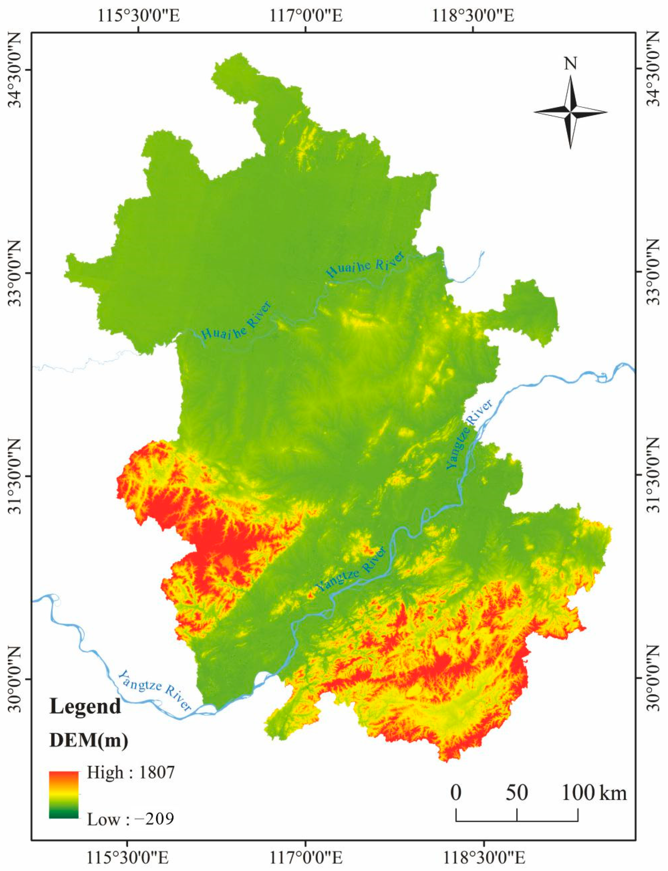
2.1. Study Area

Anhui Province is located in the Yangtze River Delta region in East China (114°54′–119°37′ E and 29°41′–34°38′ N). Anhui province is bordered by Jiangsu Province to the east, Henan Province and Hubei Province to the west, Zhejiang Province to the southeast, Jiangxi Province to the south, and Shandong Province to the north. It is 450 km wide from east to west and 570 km long from north to south, with an area of 140,100 km2. It comprises 1.45% of China’s land area. Anhui governs 16 prefecture-level cities, 59 counties (cities), and 45 municipal districts (Figure 1).
Anhui Province straddles the Yangtze River and Huaihe River Basins and is known as the land of the Yangtze River and Huaihe River. The Yangtze River and Huaihe River run from east to west, dividing the province into five natural regions: the Huaibei Plain, the Jianghuai Hills, the Riverside Plain, the Dabie Mountain region in Western Anhui, and the mountainous region in southern Anhui. The terrain is dominated by hills and mountains in the south and by plains in the north (Figure 2). There are many rivers and lakes in Anhui. The Xin’an River system in the south is part of the Qiantang River Basin; the rest is part of the Yangtze River and Huaihe River Basins. Many lakes occur along the Yangtze River and Huaihe River. Chaohu Lake is one of the five largest freshwater lakes in China, with an area of about 800 km2. The province’s resident population was 61,027,200 in 2020, ranking 9th in the country; 35,595,100 lived in towns and cities, accounting for 58.33% of the population, with an average population density of 436 people/km2. Anhui Province is an important base for agricultural products, energy, raw materials, and processing and manufacturing industries in China, generating an annual gross value of 3868.063 billion yuan, ranking 11th in the country, with a per-capita GDP of 63,426 yuan. It is an agricultural and populous province in central and eastern China, with significant differences in the population distribution and economic development levels between southern Anhui, central Anhui, and northern Anhui. Analyzing the population–economic coupling relationship and the influence of topography can provide decision support for reducing poverty and promoting urban construction in Anhui Province.

2.2. Data Sources and Processing

The data used in this study include the administrative units, socio-economic data at the county level, land-use data, and DEM. The WGS 1984 UTM Zone 50 N coordinate system is used for all data.
(1) The data related to the administrative boundaries of the study area were sourced from the National Catalogue Service for Geographic Information of China (http://www.webmap.cn/, accessed on 20 March 2023), with a scale of 1:250,000.
(2) The socio-economic data from 2020 were collected from the statistical yearbook of Anhui Province (http://tjj.ah.gov.cn/, accessed on 20 March 2023). The population density was obtained by dividing the permanent resident population of each county by the area. Similarly, the economic density was determined by dividing the GDP of each county by the area.
(3) The land-use data were obtained from the Resource and Environment Science and Data Centre of the Chinese Academy of Sciences (http://www.resdc.cn/, accessed on 25 March 2023). The land-use types in the study area include 6 primary categories and 18 secondary categories (Table 1 and Figure 3).
(4) The 30 m resolution DEM was obtained from the Geospatial Data Cloud of the Chinese Academy of Sciences (http://www.gscloud.cn/, accessed on 6 April 2023). It was used to derive elevation, slope, and topographic relief layers.

2.3. Research Framework and Methods

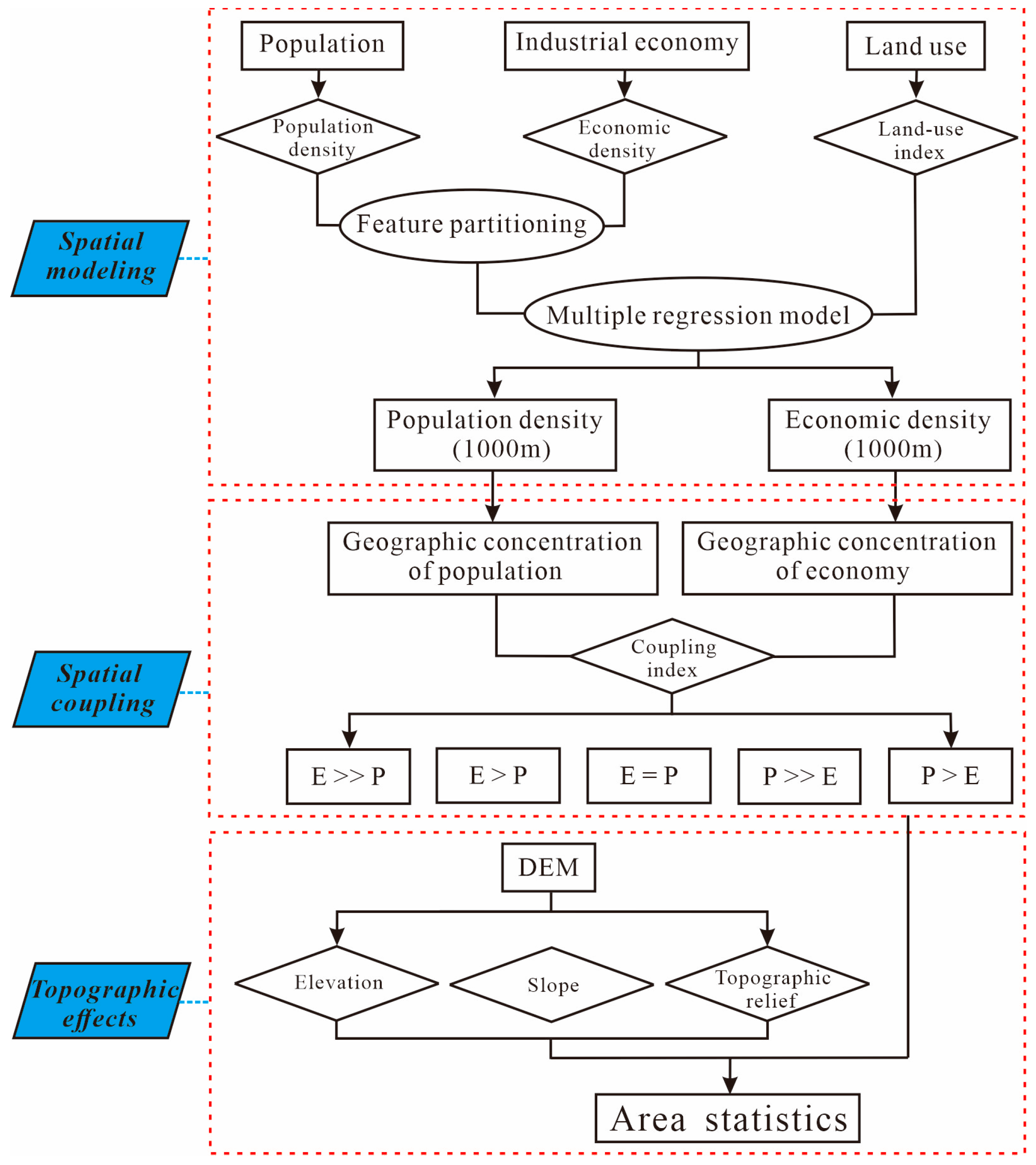
2.3.1. Research Framework

This paper used Anhui Province as the research object and spatialized the population and economic data from 2020 based on land-use data. We performed a quantitative analysis to reveal the spatial coupling relationship between population and economic densities and the influence of topography at the grid scale. A flowchart of the study is shown in Figure 4. First, we used population density and economic density as two indicators, where the population density was determined by dividing the permanent resident population of corresponding unit by the area and the economic density was determined by dividing the GDP of corresponding unit by the area, and performed grouping analysis to obtain the values of the indicators in different zones, and thus the feature partitioning was completed. Multiple regression analysis was conducted using the population and economic characteristics and the county-level population density and economic density as dependent variables and the land-use type as the independent variable. An accuracy analysis was conducted. Subsequently, the geographic concentrations of the population and economic indicators and coupling index were calculated at the grid scale. The results of the coupling index were classified into five categories: E >> P (economic polarization), E > P (economic advance), E = P (balanced development), P > E (population advance), and P >> E (population polarization), where P indicates population density and E denotes economic density. The effect of elevation, slope, and topographic relief on the population–economic spatial coupling relationship was assessed using a fitting analysis of the population density, economic density, and topographic factors. The area proportion of each coupling type for different topographic conditions was calculated.

2.3.2. Spatial Modeling of Population and Economic Data

Land use reflects human production activities and is closely related to population distribution and economic development [64,65]. A land-use impact model was constructed using multiple linear regression to assess the spatial relationship between population distribution and economic development. First, the population density and economic density were calculated, and the land use was determined in the administrative units. Significance tests were conducted, and non-significant land-use types were eliminated. A multiple linear regression model (Equation (1)) was established, with population density and economic density as the dependent variables and the land-use type as the independent variable. The area proportion of the land-use types in each grid was calculated and substituted into Equation (1) to spatialize the socio-economic data.
Y i = β 0 + β 1 X 1 i + β 2 X 2 i + + β k X k i + μ i
where Y i denotes the population and economic statistics to be spatialized, β 0 denotes the constant term, β k denotes the partial regression coefficient, X k i denotes the land-use types affecting the population and economy, and μ i denotes the residuals.

2.3.3. Analysis of the Coupling Characteristics of Population and Economy

The coupling relationship between population and economic development refers to the coordination and consistency in the spatial distribution of population and economic development. It was assessed using the geographic concentration and coupling index.
The geographic concentration is the concentration of the population and economic development in the region. It comprehensively reflects the relationship between the regional population, economy development, and area. Most existing studies calculated this index based on the administrative unit [51,52,56]. In contrast, we use grid units; thus, it is necessary to adjust the calculation formula of geographic concentration to the grid scale. It is calculated as follows:
R P O P i = P O P i / P O P i 1 / N
R G D P i = G D P i / G D P i 1 / N
where R P O P i and R G D P i , respectively, denote the geographic concentration of the population and the geographic concentration of economy in a given year for the ith grid, P O P i and G D P i , respectively, denote the number of residents and the gross regional product of the ith grid in a given year, N denotes the number of grids, and ∑ denotes the cumulative value of an attribute in the region.
Coupling index, also known as inconsistency index, is the ratio of the economic geographic concentration and the population geographic concentration in a grid unit. The calculation formula is as follows:
I i = R G D P i / R P O P i
where R P O P i and   R G D P i denote the geographic concentration of the population and the economic development level, respectively.
When I i is greater than 1, the degree of economic agglomeration is higher than the degree of population agglomeration and vice versa. When I i is equal to 1, the degree of population and economic agglomeration are comparable, i.e., balanced development is occurring. Therefore, if I i is close to 1, the levels of population distribution and economic development in the region are balanced. In contrast, the larger the deviation of I i from 1, the more significant the difference between the spatial distribution of the population and economic development in the region and the less coordinated the regional development.
Per the research of Zhao et al. [66], the values of the coupling index I for the different relationships between population and economic densities are listed in Table 2.

3. Results

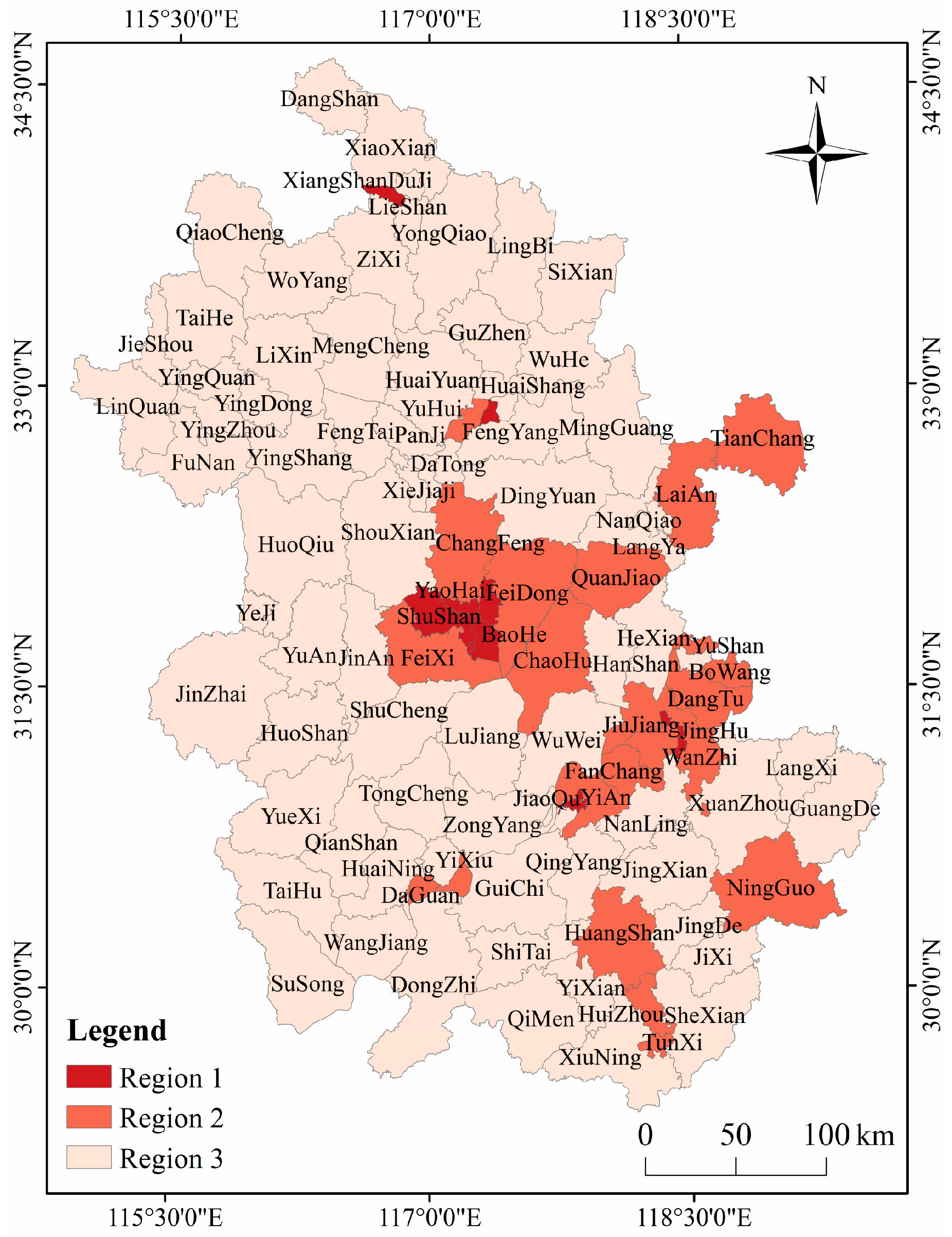
3.1. Division of Population and Economic Characteristics

Differences in natural factors and socio-economic indicators occur among regions in Anhui Province. Thus, we divided the counties (cities and districts) to improve the accuracy of population–economic spatialization. This step was performed using the grouping analysis tool in ArcGIS. The population density and economic density of each county (city and district) were taken as the grouping field, the grouping number was selected as 3, the spatial constraint was selected as no spatial constraint, and then the feature partitioning was completed. The partitioning results (Figure 5) indicate that region 1 has the most densely populated and economically developed region, including 8 units in Yaohai District, Luyang District, Shushan District, and Jinghu District. Region 2 represents areas with medium population density and economic development level, including 22 units in Feixi County, Chaohu City, and Tunxi District. Region 3 covers 71% of the county-level administrative units in Anhui Province, with the largest area and lower population density and economic density than in regions 1 and 2.

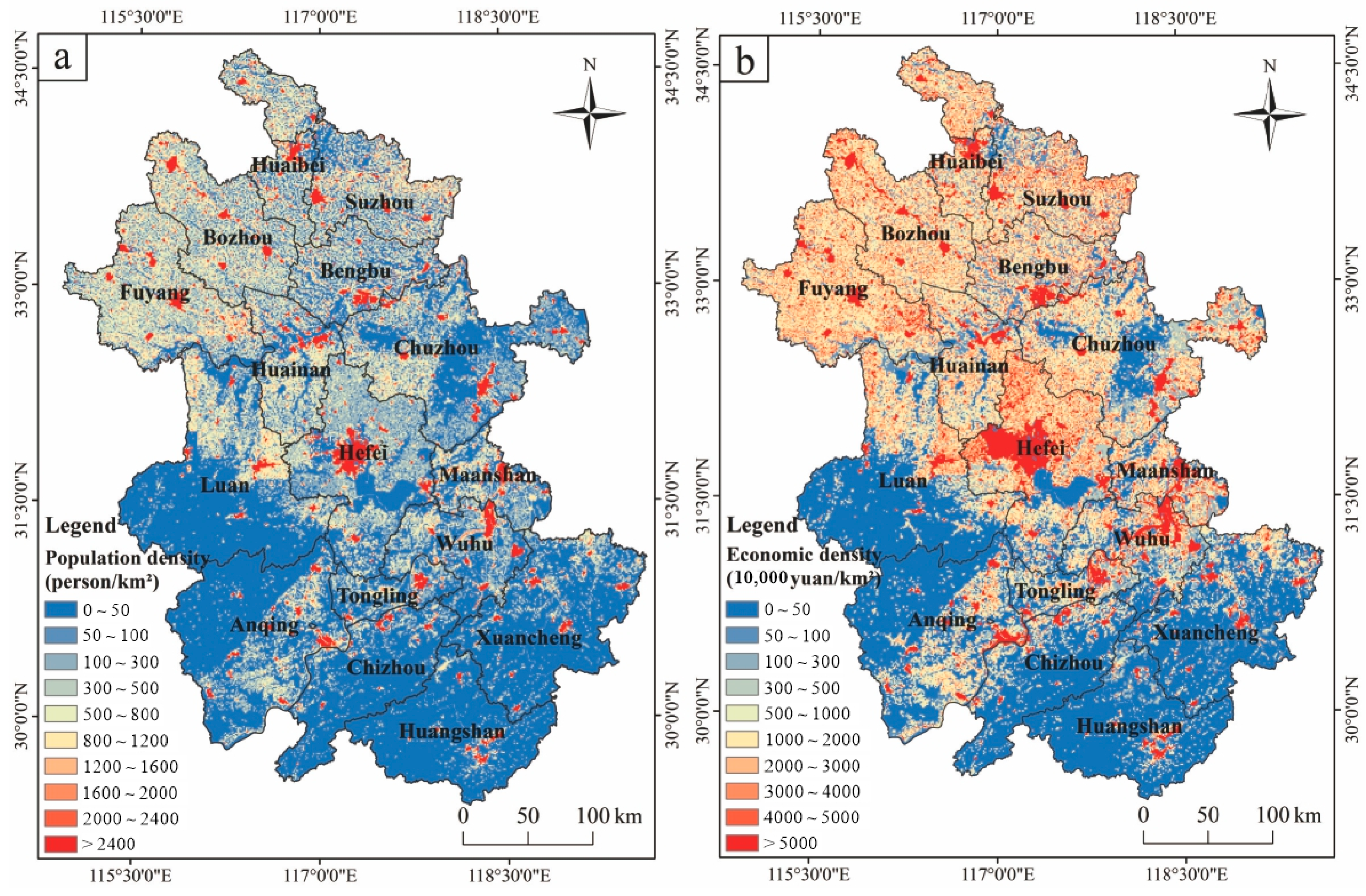
3.2. Spatialization of Population and Economic Data

3.2.1. Modeling Factor Screening

We selected land-use types with strong positive correlations with population density and economic density (Pearson correction coefficient > 0.6) as the influencing factors. The results are listed in Table 3. In the whole region, X51, X52, and X53 were selected as the spatial impact factors of population. X11, X12, and X52 were selected as the spatial impact factors of economic density for the primary industry. X51, X52, and X53 were selected as the spatial impact factors of the economic density for the secondary and tertiary industries. The selected factors of three regions are highlighted in bold in Table 3. The bold value represents the Pearson correlation coefficient > 0.6, and the corresponding land-use type indices were taken as the independent variable of the regression equation. The correlation coefficients between population density, economic density, and selected land-use type indices passed the p < 0.05 significance test.

3.2.2. Spatialized Model Construction

The multiple linear regression model was used to conduct a spatial analysis of the population density and economic density of the different zones. A large grid may result in low accuracy of results, and a small grid size causes data redundancy. Therefore, a grid size of 1000 m × 1000 m was used. The modeling steps were as follows:
(1) We calculated the land-use type index in each county. We used ArcGIS software to project the data layers (administrative boundaries and land-use data) into a unified coordinate system to overlay the data. The land-use area of the secondary class in each county unit was determined using the county name as the area field. The percentage of each secondary class land-use area in the county unit was calculated using the field calculator to obtain the land-use type index of each county unit.
(2) We constructed multiple linear regression models. We used the population density Y1, primary industry economic density Y21, and secondary and tertiary industry economic density Y22 of 104 county units as dependent variables and the screened land use type index Xij as the independent variable. SPSS software was used. We used the “Enter” method, all the selected variables (i.e., the land-use type indices with Pearson’s correlation coefficient > 0.6 with population density and economic density) were included in the regression model. We selected the ordinary least square (OLS) estimator to calculate the regression equation. According to the principle of “no land use, no population and economy”, the constant term in the fitting equation was set to 0. Thus, the fitting equations characterizing the spatial distribution of the population and economic density were derived. The results are listed in Table 4. All variables in the regression equations passed the p < 0.05 significance t-test, and all regression equations passed the F-test, indicating that the linear relationship is globally significant, and the results are statistically significant. The Adj. R2 of the regression equations for the regions were generally better than that of the regression equations for the whole region. Thus, the former better reflect the differences in the population distribution and economic development in different regions, demonstrating the rationality of using different zones for spatial modeling of population distribution and economic development.
(3) We calculated the population and economic densities at the grid scale. We created a 1000 m × 1000 m grid and overlaid it with the land-use data to calculate the proportion of different land-use types in the grid area and generate a new attribute field. We used the regression coefficients of each category from Table 3 and used the field calculator to obtain the regression value representing the population and economic densities in each grid. It should be pointed out that some negative values were obtained in the regression analysis. We changed the negative values to zero. Finally, the regression results were mapped to complete the gridding of the population and economic data (Figure 6). We performed regression analyses separately for primary, secondary, and tertiary industries and overlaid the results to obtain the economic density of Anhui Province.
Figure 6 shows that the population and economy densities in Anhui Province are higher in the north and lower in the south. Most of the population is concentrated in municipal districts, and the economic density is high in the municipal districts and the vicinity of the two major rivers, the Yangtze River and the Huaihe River. The topography of Anhui Province is low in the north and high in the south. The flatter northern part is conducive to population aggregation and economic development. The southern part of the province is predominantly mountainous and hilly areas, and the complex topographic conditions have hindered population and economic development. The Yangtze River and the Huaihe River are critical for water transportation and traffic and contribute to economic development; thus, areas close to the river have high economic density. As the capital city of Anhui Province, Hefei is a central city in the Yangtze River Delta Urban Agglomeration and has a dense population and well-developed economy. In addition, the population distribution and economic development are uneven in Anhui Province, resulting in significant regional development differences.
In addition, a coupling relationship between population density and economic density is observed in the spatial pattern. Further correlation analysis results show that the fitting coefficients R2 between population density and economic density are 0.608, 0.909, and 0.890 in region 1, region 2, and region 3 (p < 0.01), respectively, indicating a strong positive correlation and coordination between the population and economic densities. However, there are differences in the coordination of different regions. The fitting accuracy between population and economic densities is lower in region 1 than in the other two regions, but the coordination of the two parameters is weak in terms of spatial distribution. Region 2 has the highest fitting accuracy of population and economic densities, and Region 3 has a slightly lower accuracy. These results indicate that the population and economic densities in this region are similar, and the coordination between the parameters is high. However, the population and economic densities are lower than in region 1.

3.2.3. Accuracy Verification

To verify the reliability and accuracy of the regression model, the actual values of population density, economic density, and economic density of each industry were linearly fitted with spatially predicted values. The fitting results passed the p < 0.01 significance test. Figure 7 shows that the fitting accuracy R2 between the actual and predicted population density and economic density in the primary, secondary, and tertiary industries are 0.974, 0.942, 0.893, and 0.941, respectively, indicating the high accuracy of the proposed land-use impact model. The predicted grid-based population density and economic density are highly similar to the actual values in Anhui Province.

3.3. Spatial Coupling Characteristics of Population and Economy

The maps of the population–economic density coupling index (Figure 8a) and the area proportion of the five types in each county (Figure 8b) show substantial regional differences in the index in Anhui Province. The following is observed: (1) High values of coupling index occur in strips and masses. The strips include high-value areas along the Huaihe River, the Hefei–southern Chuzhou region, and areas along the Yangtze River. The masses of high-value areas include the Huangshan–Jiuhuashan Scenic Area and the whole Ningguo area. The E >> P and E > P types are dominant in the high-value areas, which have better geographic locations, convenient water and railroad transportation, and a favorable national policy, resulting in the high economic development of the Hefei metropolitan area, the Wangjiang River Economic Belt, and the Jiangzhe Economic Circle. However, its population development is lagging behind its economic development. (2) The median area of the coupling index occurs in the southern Anhui region and the Dabie Mountain region in western Anhui, including Huangshan, Chizhou, Xuancheng, southern Lu’an, and northern Anqing. The region has benefited from tourism, improvements to the transportation network, and increasingly convenient external exchange. However, the external exchange of the region is dominated by tourism, the leading industry. The industrial structure is less developed, and the level of economic development is relatively low. The complex topographic conditions represent a barrier to population growth. Balanced development type (E = P) is dominant in this area, i.e., the population density is comparable to the level of economic development, but population density and economic level are lower than in other regions. (3) The low-value areas of the coupling index occur in northern Anhui, especially in northwestern Anhui, including Fuyang, Bozhou, northern Lu’an, and Huainan. The P > E type is dominant in this region, with few areas of the P >> E type. The region has rich coal resources, and the flat topographic conditions facilitate resource development and utilization. Therefore, the population density in the region was high in the early stage of national development. However, resource depletion and floods on both sides of the Huaihe River due to the diversion of the Yellow River caused a mismatch between the economic development rate and the population growth rate in the northern Anhui region, resulting in unbalanced development of the population and the economy.

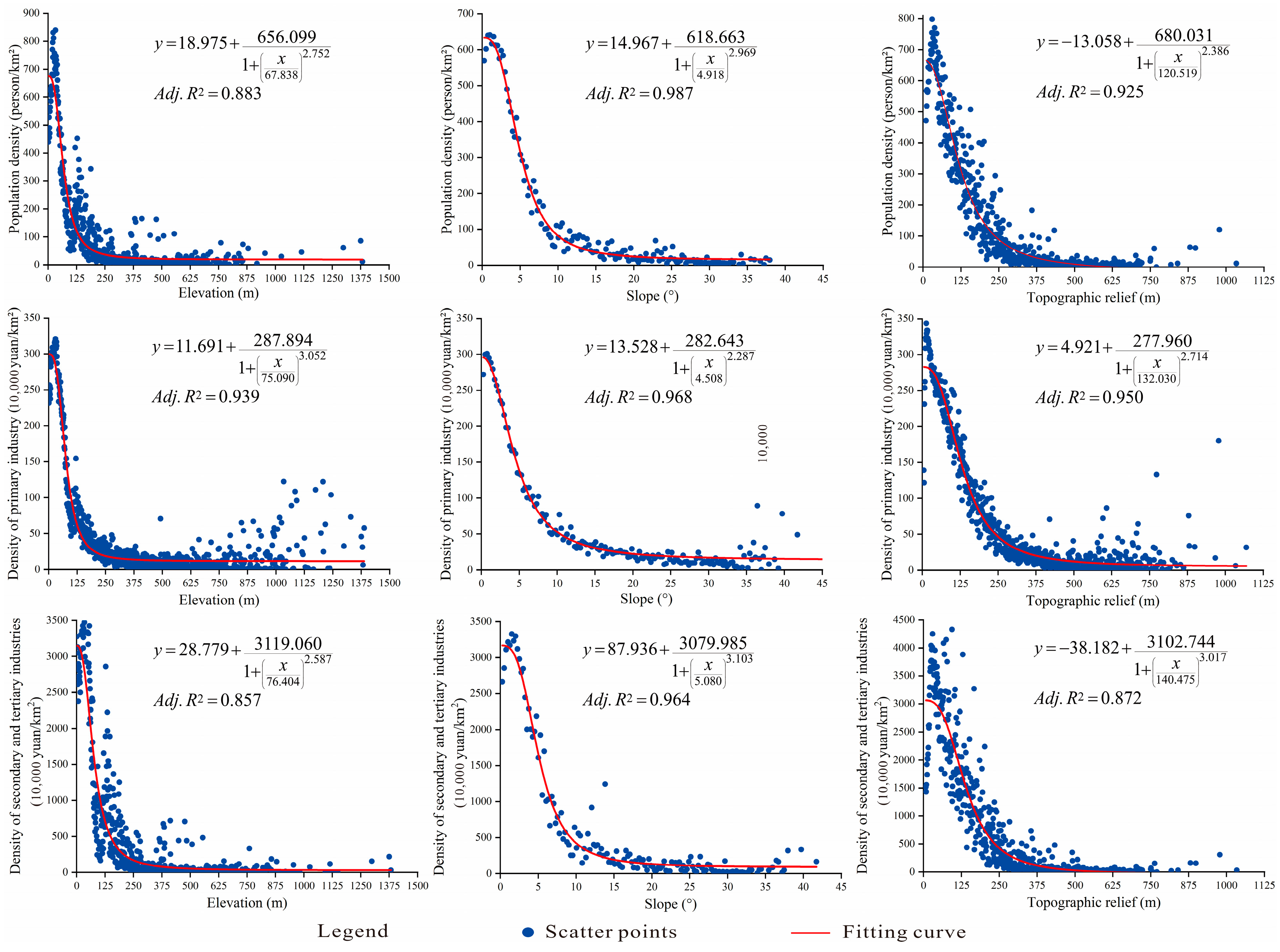
3.4. Topographic Effect of Population Distribution and Economic Development

Based on the distribution pattern of density-topographic scatter space, a logistic function was used to carry out nonlinear fitting, and the significance level p = 0.05. Figure 9 shows the effects of elevation, topographic relief, and slope on population and economic densities. All topographic factors have similar effects on population density and economic density, showing strong negative correlations. Slope has the strongest effect on population density and economic density, followed by topographic relief and elevation. The correlation is higher between topographic factors and population density and primary industry density than between the topographic factors and secondary and tertiary industry density. The reason is that primary industry includes agriculture, forestry, animal husbandry, and fishery, which have a high degree of dependence on the natural environment. In contrast, secondary and tertiary industries include industry, manufacturing, and service, which have a relatively low degree of dependence on the natural environment.
We used the grading standards of Chinese digital geomorphological mapping and considered the conditions in the study area to divide the elevation range into 10 levels, the slope into 5 levels, and the degree of topographic relief into 5 levels. Table A1 indicates that population density and economic density decrease as elevation, slope, and topographic relief increase. In regions with elevations < 100 m, the proportion of the population size and the proportion of the total economy are 96.96% and 97.08%, respectively. In regions with slopes < 6°, the proportion of the population size and the proportion of the total economy are 96.77% and 96.66%, respectively. In regions with topographic relief < 70 m, the proportion of the population size and the proportion of the total economy are 87.14% and 85.24%, respectively. This result shows that the population density and economic development of Anhui Province are higher in regions with low elevation, slope, and topographic relief.

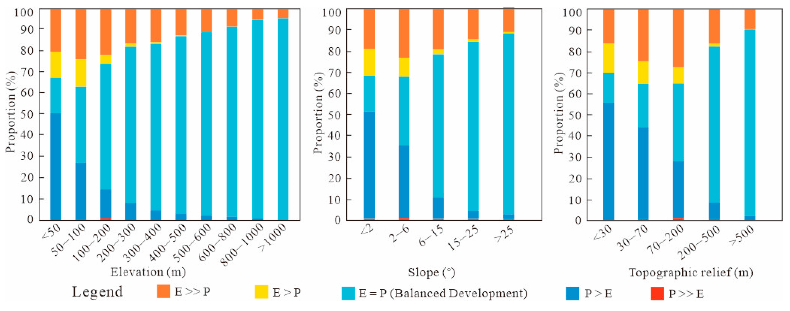
3.5. Topographic Effect on the Spatial Coupling Index

Anhui Province has a wide range of topography and geomorphology, with plains, hills, and mountains occurring from north to south. The complex topographic features are one reason for the regional differences in population density and economic development in Anhui Province. As shown in Figure 10, a correlation exists between the five relationship types and topography. Specifically, the area proportion of the E >> P type increases and decreases as three topographic factors increase but is generally negatively correlated with topography, while the area proportion of the E > P type is negatively correlated with topography. The area proportion of the balanced development type has a positive correlation with topography. The area proportion of the P >> E type is very small, and the area proportion of the P > E type is significantly and negatively correlated with topography.
As elevation increases, the area proportion of the E >> P type increases from 20.76% to 24% and then decreases to 3.33%; the area proportion of the E > P type increases from 11.75% to 12.87% and decreases to 0%; the area proportion of the balanced development type increases from 16.61% to 96.67%; the area proportion of the P > E type decreases from 50.38% to 0%; and the area proportion of the P >> E type increases from 0.5% to 1.05% and then decreases to 0%. As slope increases, the area proportion of the E >> P type increases 19.51% to 24.02% and then decreases to 11.5%; the area proportion of the E > P decreases from 12.66% to 0.57%; the area proportion of the balanced development type increases from 16.77% to 85.02%; the area proportion of the P > E type decreases from 50.6% to 2.51%; and the area proportion of the P << E type increases from 0.45% to 0.77% and then decreases to 0.39%. As topographic relief increases, the area proportion of the E >> P type increases from 16.43% to 24.6% and then decreases to 9.48%; the area proportion of the E > P type decreases from 13.78% to 0.21%; the area proportion of the balanced development type increases from 14.08% to 88.33%; the area proportion of the P > E type decreases from 55.4% to 1.87%; and the area proportion of the P >> E type increases from 0.32% to 1.06% and then decreases to 0.1%.
The influence of topography on population distribution and the economic development of primary, secondary, and tertiary industries is characterized by the following. (1) Regions with relatively flat topography are more conducive to large-scale population aggregation and industry infrastructure, facilitating the development of the primary industry economy. Thus, this region attracts investment, promoting the development of secondary and tertiary industries. Therefore, these regions have larger proportions of the E > P, E >> P, and P > E types. (2) A region with complex and steep topography is not conducive to high population density, prevents the extensive use of mechanized agriculture, and hinders the development of the primary industry economy. Investors are reluctant to invest in these regions, resulting in the limited development of the secondary and tertiary industries; thus, the area of the balanced development type is relatively large. (3) Flat topography and rich coal resources have caused lower economic development in northern Anhui. Its economic density lags behind its population density. The region is far from the economic center and relies primarily on primary industry and coal resources for development. The industrial structure is imbalanced, and resource exploitation has caused significant environmental damage. The production capacity is low, resulting in limited economic development. Long-term population increase has resulted in relatively high population density in northern Anhui. (4) Although coupling between population and economic densities has occurred in regions with complex topography, the population and economic densities are much lower in these regions than in areas with flat topography (Table A1), and the regional economic development is relatively low. The unbalanced economic development of the southern Anhui region and the Dabie Mountain region in the western and northern Anhui regions has restricted economic development in Anhui Province. The government should formulate precise poverty alleviation policies, focusing on labor skills training to stimulate the motivation of the working population. It should implement measures to increase income and improve the regional economic development level.

4. Discussion

4.1. Comparison of Administrative Units and Grid Units

Many researchers have investigated the spatial distribution and coordinated development of the population and economy in Anhui Province. Wei et al. [67] used prefecture-level cities as statistical units and used descriptive statistics, econometric models, and GIS to analyze the evolution and coupling coordination of the population distribution and regional economic differences in Anhui Province. They used data from the fifth national population census in 2020 to the sixth national population census in 2010. The results showed that population density lagged behind economic density in the central Anhui region, represented by Hefei, Wuhu, and Maanshan. Population and economic densities were more coordinated in southern Anhui, represented by Xuancheng, Huangshan, and Anqing, and population density exceeded economic density in northern Anhui, represented by Fuyang, Bozhou, and Suzhou. Wen et al. [68] analyzed the spatiotemporal evolution pattern of population and economic development in prefecture-level cities in Anhui Province from 2000 to 2015. They assessed the imbalance of population and economic development using coupling index. The results showed that cities with higher economic development were concentrated in central Anhui, cities with coordinated population and economic development were located in eastern and southern Anhui, and most cities with low economic development occurred in western and northern Anhui. Wang et al. [69] used county population and economic data from 1998 to 2015 and revealed the spatiotemporal coupling characteristics of the population–economic system in Anhui Province utilize geostatistics. The analysis showed that the economic development speed of northern and southern Anhui was relatively slow, whereas central Anhui was the core of economic development in Anhui Province. The population decreased from northern Anhui to central and southern Anhui. Dai et al. [70] obtained county population and economic data from 2002 to 2017 and systematically analyzed the spatial evolution of coordinated development between population and economy. The result showed that the economic density effect was more pronounced in central Anhui, but the pulling effect on the population was not large. Therefore, population density lagged behind economic density and was higher in northern and western Anhui. However, the economic development of the dominant industry was low; thus, population density was higher than economic density.
The results of previous studies were consistent with our results, indicating the reliability of our findings. However, most existing studies utilized socio-economic statistics of counties or municipal administrative units, reflecting the spatial distribution of population and economic density in these units without examining spatial differences within the administrative units. In addition, the topography of the Dabie Mountain region in southern and western Anhui is complex, exacerbating these differences. The grid-based scale used in this study provides more accurate data on the relationship between population and economic densities within administrative units, especially in regions with complex topography. Thus, this approach is superior to the one used in existing studies.

4.2. Grid-Scale Effects of the Spatialization of Population and Economic Data

Most spatialized products of socio-economic statistics are based on 1-km grid datasets (Global Rural–Urban Mapping Project (GRUMP), Land-Scan, and the China Kilo-meter Gridded Population Dataset (OpenGMS)) or 5-km grid datasets (the United Nations Environment Program’s Global Resource Information Database (UNEP/GRID) and the Gridded Population of the World (GPW)). Several smaller-scale grid datasets, such as WorldPop (100 m), also exist. Although these data have higher spatial resolution than statistical data, no studies have assessed suitable grid scales for different regions. Li et al. [71] stated that geographical objects are scale-dependent and suitable grids have unique characteristics, i.e., temporal, spatial, or spatiotemporal. Different grid scales significantly impact the accuracy of spatialization of socio-economic statistics. However, existing studies did not fully consider the differences in population distribution and economic development in different regions and seldom considered the effect of the grid scale on spatialization.
Two methods are commonly used to evaluate grid scale suitability. The first is based on source data and includes variograms [72] and the assessment of remote sensing image response relationships [73]. The second type includes statistical methods and variance analysis [74]. Several scholars have proposed an index system evaluation method using landscape ecology indicators, such as the shape index, to analyze the scale effect of population distribution [75]. Others have determined appropriate grid scale by using multiple indices related to spatial relationships and distributions and numerical analysis [76,77].
Therefore, it is necessary to analyze the distribution pattern of population and economic densities at different scales to determine the appropriate grid scale for specific regions. In addition, a more reasonable accuracy analysis method should be developed to evaluated the grid scale suitability to express the spatial distribution of population and economic densities at different scales.

5. Conclusions

Population and economic data of Anhui Province in 2020 and grouping analysis were used to classify the population and economic densities. A land-use impact model was selected to spatialize the socio-economic indicators, determine the relationship between population and economic densities, and assess the effect of topography quantitatively using grid units. The main conclusions are as follows:
(1) Modeling accuracy was higher when different zones were considered instead of the whole area. The population and economic densities predicted by the spatialization model exhibited a good fit with the statistical values, indicating that the proposed method accurately predicted population distribution and economic development. Population and economic densities had similar spatial distribution patterns. The coupling index was classified into five types: E >> P, E > P, E = P (balanced development), P > E, and P >> E. The balanced development type was dominant in southern Anhui and the Dabie Mountain region in western Anhui, indicating balanced development between the population distribution and economic development. The P > E and P >> E types occurred in northern Anhui, with economic aggregation lagging behind population aggregation. The E > P and E >> P types were dominant in central Anhui, with economic aggregation being greater than population aggregation.
(2) Topographic factors had a stronger effect on population and primary industry than on secondary and tertiary industries. Slope had the strongest effect on population density, followed by topographic relief and elevation. Complex topographic areas with elevations > 100 m, slopes > 6, and topographic relief > 70 m were dominant in the mountainous regions in southern Anhui and the Dabie Mountain region in western Anhui. Although population and economic densities exhibited coordinated development, both densities were much lower in this region than in flatter regions.
(3) The population–economy spatial relationship was correlated with topographic factors. As elevation, slope, and topographic relief increased, the proportion of the balanced area increased, and the proportion of the remaining four types showed different degrees of decline. Complex topographic conditions had a significant barrier effect on population growth and economic development, resulting in areas with complex topography exhibiting balanced population–economic development. In addition, the northern Anhui region, with its flat topography, has a large population base due to the long-term influx of people, and economic development lagged behind population aggregation. Efforts should be made to improve the economic level of the southern and northern Anhui regions and the Dabie Mountain region in western Anhui.
However, there are also some deficiencies in our research, which may affect the accuracy and applicability of some conclusions in this paper, specifically: (1) Considering the convenience of spatial modeling and application, this paper only adopts a single-scale land-use type as a modeling factor to spatialize the county population and sub-industry economic data; it can consider using land-use type data of different classification categories and different scales to compare and analyze its impact on the spatialization results in the future. (2) Only the cross-sectional data of a single year was used to explore the spatial coupling relationship between population and economy, which is lacking in terms of the spatial dynamic change process, and the result may be accidental. In the future, multi-year panel data should be collected for analysis to discuss the population change and economic development trend, so as to improve the persuasiveness and practical value of the results. (3) The spatial variation characteristics of socio-economic and topographic elements are scale-dependent, which is not explored in depth in this paper, and needs to be strengthened and improved.

Author Contributions

Conceptualization, Z.Y.; methodology, Z.Y. and Y.H.; software, Y.H.; validation, Z.Y. and G.Z.; formal analysis, S.W. and M.Z.; resources, Z.Y. and Y.H.; data curation, Y.H. and Z.Y.; writing—original draft preparation, Z.Y. and Y.H.; writing—review and editing, Z.Y. and G.Z.; visualization, Z.Y. and Y.H.; supervision, Z.Y. and C.L.; project administration, Z.Y. and X.Y.; funding acquisition, Z.Y. and X.Y. All authors have read and agreed to the published version of the manuscript.

Funding

This research was funded by the Open Foundation of the Key Laboratory of Aviation–Aerospace–Ground Cooperative Monitoring and Early Warning of Coal Mining-Induced Disasters of Anhui Higher Education Institutes (Anhui University of Science and Technology), grant number KLAHEI202208, the Anhui University of Science and Technology Doctoral Talent Introduction Foundation, grant number 201711936, the Anhui Provincial Natural Science Foundation, grant number 2208085MD88, Anhui Province Science and Technology Major Science and Technology Project, grant number 202103a05020026, and the Anhui Provincial Key Research and Development Project, grant number 202104a07020014.

Data Availability Statement

Publicly available datasets were analyzed in this study. The data are available from the following sources: the National Catalogue Service for Geographic Information of China [online], http://www.webmap.cn/, (accessed on 20 March 2023); Statistical yearbook of Anhui Province [online], http://tjj.ah.gov.cn/, (accessed on 20 March 2023); Resource and Environment Science and Data Centre of the Chinese Academy of Sciences [online], http://www.resdc.cn/, (accessed on 25 March 2023); Geospatial Data Cloud of the Chinese Academy of Sciences [online], http://www.gscloud.cn/, (accessed on 6 April 2023).

Conflicts of Interest

The authors declare no conflict of interest.

Appendix A

Table A1. Population and economic statistics for different elevations, slopes, and topographic reliefs.
Topographic FactorLevelPopulation Density/(Persons per km−2)Economic Density/(10,000 Yuan·km−2)Size of the PopulationGross Domestic Production (GDP)
Sum/10,000 PersonRatio/%Sum/Billion YuanRatio/%
Elevation/(m)<50645.72 3502.65 5776.59 90.61 31,334.69 89.11
50~100300.33 2077.93 404.81 6.35 2800.84 7.97
100~200143.56 787.72 149.23 2.34 818.83 2.33
200~30036.42 170.82 27.02 0.42 126.71 0.36
300~40017.24 79.22 9.27 0.15 42.60 0.12
400~50011.92 54.92 4.76 0.07 21.95 0.06
500~6007.26 29.85 1.97 0.03 8.08 0.02
600~8004.53 18.17 1.51 0.02 6.05 0.02
800~10002.43 11.66 0.35 0.01 1.69 0.00
>10001.62 33.88 0.05 0.00 0.84 0.00
Slope/(°)<2621.70 3414.89 4861.98 76.29 26,705.80 75.98
2~6481.89 2682.81 1305.45 20.48 7267.72 20.68
6~1599.49 574.94 164.73 2.58 951.93 2.71
15~2529.90 158.71 35.96 0.56 190.88 0.54
>2511.08 70.65 5.01 0.08 31.98 0.09
Topographic Relief/(m)<30644.86 3495.80 3367.12 52.71 18,253.30 51.82
30~70653.29 3496.28 2199.75 34.43 11,772.69 33.42
70~200331.68 2101.14 695.43 10.89 4405.46 12.51
200~50047.86 301.47 123.39 1.93 777.32 2.21
>5004.37 22.91 2.90 0.05 15.18 0.04

References

  1. Verbavatz, V.; Barthelemy, M. The growth equation of cities. Nature 2020, 7834, 397–401. [Google Scholar] [CrossRef] [PubMed]
  2. Wiedmann, T.; Allen, C. City footprints and SDGs provide untapped potential for assessing city sustainability. Nat. Commun. 2021, 1, 3758. [Google Scholar] [CrossRef]
  3. Adam, S. The Wealth of Nations; Random House Inc.: New York, NY, USA, 1994. [Google Scholar]
  4. Jiang, L.; Deng, X.; Seto, K.C. Multi-level modeling of urban expansion and cultivated land conversion for urban hotspot counties in China. Landsc. Urban Plan. 2012, 41, 131–139. [Google Scholar] [CrossRef]
  5. Hu, H.Y.; Zhang, S.Y. Essays on China’s Population Distribution; East China Normal University Press: Shanghai, China, 1986. [Google Scholar]
  6. Zhong, Y.X.; Lu, Y.Q. The coupling relationship between population and economic in Poyang lake ecological economic zone. Econ. Geogr. 2011, 31, 195–200. [Google Scholar]
  7. Wang, D.H.; Li, X.D. Coordination of population and economic development in the Wujiang river basin of Guizhou province. Sci. Geogr. Sin. 2019, 39, 477–486. [Google Scholar]
  8. Wu, J.D.; Wang, X.; Wang, C.L.; He, X.; Ye, M.Q. The status and development trend of disaggregation of socio-economic data. J. Geo-Inf. Sci. 2018, 20, 1252–1262. [Google Scholar]
  9. Bai, Z.Q.; Wang, J.L.; Yang, F. Research progress in spatialization of population data. Prog. Geogr. 2013, 32, 1692–1702. [Google Scholar]
  10. Roy, D.; Palavalli, B.; Menon, N.; King, R.; Pfeffer, K.; Lees, M.; Sloot, P.M.A. Survey-based socio-economic data from slums in Bangalore, India. Sci. Data 2018, 5, 170200. [Google Scholar] [CrossRef]
  11. Dong, N.; Yang, X.H.; Cai, H.Y. Research progress and perspective on the spatialization of population data. J. Geo-Inf. Sci. 2016, 18, 1295–1304. [Google Scholar]
  12. Zhang, J.J.; Zhu, W.B.; Zhu, L.Q.; Cui, Y.P.; He, S.S.; Ren, H. Spatial variation of terrain relief and its impacts on population and economy based on raster data in west Henan mountain area. Acta Geogr. Sin. 2018, 73, 1093–1106. [Google Scholar]
  13. Lu, X.; Li, J.; Duan, P.; Cheng, F.; Wang, J.L. Spatialization and forecasting of GDP in Yunnan border area based on nighttime light and land use data. Areal Res. Dev. 2020, 39, 36–39. [Google Scholar]
  14. Igor, K. Geostatistics portal-an integrated system for the dissemination of geo-statistical data. Statistika 2013, 93, 100–108. [Google Scholar]
  15. Li, F.; Zhang, S.W.; Yang, J.C.; Wang, Q. A review on research about spatialization of socioeconomic data. Geogr. Geo-Inf. Sci. 2014, 30, 102–107. [Google Scholar]
  16. Yazdian, H.; Salmani, D.N.; Alijanian, M. A spatially promoted SVM model for GRACE downscaling: Using ground and satellite-based datasets. J. Hydrol. 2023, 626, 130214. [Google Scholar] [CrossRef]
  17. Guo, H.X.; Zhu, W.Q. A review on the spatial disaggregation of socioeconomic statistical data. Acta Geogr. Sin. 2022, 77, 2650–2667. [Google Scholar]
  18. Velpuri, N.M.; Senay, G.B.; Singh, R.K.; Bohms, S.; Verdin, J.P. A comprehensive evaluation of two MODIS evapotranspiration products over the conterminous United States: Using point and gridded FLUXNET and water balance ET. Remote Sens. Environ. 2013, 139, 35–49. [Google Scholar] [CrossRef]
  19. Zhang, J.J.; Zhu, W.B.; Zhu, L.Q.; Cui, Y.P.; He, S.S.; Ren, H. Topographical relief characteristics and its impact on population and economy: A case study of the mountainous area in western Henan, China. J. Geogr. Sci. 2019, 29, 598–612. [Google Scholar] [CrossRef]
  20. Luo, J.; Shi, P.J.; Zhang, X.B. Relationship between topographic factors and population distribution in Lanzhou-Xining urban agglomeration. Econ. Geogr. 2020, 40, 106–115. [Google Scholar]
  21. Ustaoglu, E.; Williams, B. Institutional settings and effects on agricultural land conversion: A global and spatial analysis of European regions. Land 2022, 12, 47. [Google Scholar] [CrossRef]
  22. Alahmadi, M.; Mansour, S.; Martin, D.; Atkinson, P.M. An improved index for urban population distribution mapping based on nighttime lights (DMSP-OLS) data: An experiment in Riyadh Province, Saudi Arabia. Remote Sens. 2021, 13, 1171. [Google Scholar] [CrossRef]
  23. Kumar, P.; Sajjad, H.; Joshi, P.K.; Elvidge, C.D.; Rehman, S.; Chaudhary, B.S.; Tripathy, B.R.; Singh, J.; Pipal, G. Modeling the luminous intensity of Beijing, China using DMSP-OLS night-time lights series data for estimating population density. Phys. Chem. Earth 2019, 109, 26–34. [Google Scholar] [CrossRef]
  24. Bakillah, M.; Liang, S.; Mobasheri, A.; Arsanjani, J.J.; Zipf, A. Fine-resolution population mapping using OpenStreetMap point-of-interest. Int. J. Geogr. Inf. Sci. 2014, 28, 1940–1963. [Google Scholar] [CrossRef]
  25. Yeow, L.W.; Low, R.; Tan, Y.X.; Cheah, L. Point-of-Interest (POI) data validation methods: An urban case study. ISPRS Int. J. Geo-Inf. 2021, 10, 735. [Google Scholar] [CrossRef]
  26. Jonietz, D.; Zipf, A. Defining fitness-for-use for crowdsourced Points of Interest (POI). ISPRS Int. J. Geo-Inf. 2016, 5, 149. [Google Scholar] [CrossRef]
  27. Deville, P.; Linard, C.; Martin, S.; Gilbert, M.; Stevens, F.R.; Gaughan, A.E.; Blondel, V.D.; Tatem, A.J. Dynamic population mapping using mobile phone data. Proc. Natl. Acad. Sci. USA 2014, 111, 15888–15893. [Google Scholar] [CrossRef] [PubMed]
  28. Kubícek, P.; Konecny, M.; Stachon, Z.; Shen, J.; Herman, L.; Rezník, T.; Stanek, K.; Stampach, R.; Leitgeb, S. Population distribution modelling at fine spatio-temporal scale based on mobile phone data. Chem. Eng. J. 2019, 12, 1319–1340. [Google Scholar] [CrossRef]
  29. Wu, Z.Y.; Xu, H.W.; Hu, Z.M. Fine-scale population spatialization based on Tencent location big data: A case study of Moling subdistrict, Jiangning district, Nanjing. Geogr. Geo-Inf. Sci. 2019, 35, 61–65. [Google Scholar]
  30. Li, H.M.; Luo, D.W.; Dou, S.Q. The estimation of population on multi-spatial scale using Tencent location big data. Bull. Surv. Mapp. 2022, 6, 93–97. [Google Scholar]
  31. Muhammad, R.; Wanggen, W.; Ofelia, C.; Luc, G. Using location based social media data to observe check in behavior and gender difference: Bringing Weibo data into play. ISPRS Int. J. Geo-Inf. 2018, 7, 196. [Google Scholar]
  32. Kuang, W.H.; Du, G.M. Analyzing urban population spatial distribution in Beijing proper. J. Geo-Inf. Sci. 2011, 13, 506–512. [Google Scholar] [CrossRef]
  33. Zhang, C.F.; Qiu, F. A point-based intelligent approach to areal interpolation. Prof. Geogr. 2011, 62, 262–276. [Google Scholar] [CrossRef]
  34. Weng, C.Y.; Xin, G.X.; Yang, Q.Y. Building of a spatialization model of socioeconomic data in mountainous and hilly regions and its application. J. Southwest Univ. Nat. Sci. Edit. 2018, 40, 96–103. [Google Scholar]
  35. Yue, T.X.; Wang, Y.A.; Chen, S.P.; Liu, J.Y.; Qiu, D.S.; Deng, X.Z.; Liu, M.L.; Tian, Y.Z. Numerical simulation of population distribution in China. Popul. Environ. 2003, 25, 141–163. [Google Scholar] [CrossRef]
  36. Cheng, F.L.; Zhao, G.W. Fine-scale simulation of population distribution based on zoning strategy and machine learning. Sci. Surv. Mapp. 2020, 45, 165–173. [Google Scholar]
  37. Townsend, A.C.; Bruce, D.A. The use of night-time lights satellite imagery as a measure of Australia’s regional electricity consumption and population distribution. Int. J. Remote Sens. 2010, 31, 4459–4480. [Google Scholar] [CrossRef]
  38. Zheng, H.H.; Gui, Z.P.; Wu, H.Y.; Song, A.H. Developing non-negative spatial autoregressive models for better exploring relation between nighttime light images and land use types. Remote Sens. 2020, 12, 798. [Google Scholar] [CrossRef]
  39. Morshed, M.M.; Chakraborty, T.; Mazumder, T. Measuring Dhaka’s urban transformation using nighttime light data. J. Geovis. Spat. Anal. 2022, 6, 25–37. [Google Scholar] [CrossRef]
  40. Chen, Q.; Hou, X.Y.; Wu, L. Comparing of population spatialization models based on land use data and DMSP/OLS data respectively: A case study in the efficient ecological economic zone of the yellow river delta. Hum. Geogr. 2014, 29, 94–100. [Google Scholar]
  41. Huang, Y.H.; Zhao, C.P.; Song, X.Y.; Chen, J.; Li, Z.H. A semi-parametric geographically weighted (S-GWR) approach for modeling spatial distribution of population. Ecol. Indic. 2018, 85, 1022–1029. [Google Scholar] [CrossRef]
  42. Fan, J.; Tao, A.J.; Lv, C. The coupling mechanism of the centroids of economic gravity and population gravity and its effect on the regional gap in China. Prog. Geogr. 2010, 29, 87–95. [Google Scholar]
  43. Gaughan, A.E.; Stevens, F.R.; Linard, C.; Jia, P.; Tatem, A.J. High Resolution population distribution maps for Southeast Asia in 2010 and 2015. PLoS ONE 2013, 8, 55882. [Google Scholar] [CrossRef] [PubMed]
  44. He, S.S.; Fang, B. Population-economy coupling and its effect on topographic gradients in Anhui province, China based on a grid scale. Tropi. Geogr. 2021, 41, 351–363. [Google Scholar]
  45. Julian, L.S. Population Growth Economics; Peking University Press: Beijing, China, 1984. [Google Scholar]
  46. George, H.; Evangelia, P. Demographic changes, labor effort and economic growth: Empirical evidence from Greece. J. Policy Model. 2001, 23, 169–188. [Google Scholar]
  47. Garza, R.J.; Andrade, V.C.; Martinez, S.K.; Renteria, R.F.; Vallejo, C.P. The Relationship Between Population Growth and Economic Growth in Mexico. Soc. Sci. Electron. Publ. 2016, 36, 97–107. [Google Scholar]
  48. Zhang, J.W.; Gao, C.; Zhao, J. Research on the changing spatial gravity of China’s population, economy, and industry center: Based on the provincial data from 1978 to 2019. Chin. J. Popul. Sci. 2021, 1, 64–78. [Google Scholar]
  49. Liang, L.W.; Xian, Y.; Chen, M.X. Evolution trend and influencing factors of regional population and economy gravity center in China since the reform and opening-up. Econ. Geogr. 2022, 42, 93–103. [Google Scholar]
  50. Xiao, Z.Y.; Guo, G.H. Research on the coordinated evolution of population, economy and environment in the Yangtze River Delta. Environ. Sci. Technol. 2021, 44, 196–205. [Google Scholar]
  51. Zhao, M.; Di, D.R.; Huang, G.W.; Shi, W.Y. Evolution and coupling between economic and population spatial pattern in Wujiang river basin. Res. Soil Water Conserv. 2022, 29, 298–310. [Google Scholar]
  52. Lv, D.H.; Zhang, Y.; Liu, Y.Q. Spatial coupling relationship between rural population and economy under the background of rural shrinkage in Songnen plain. Econ. Geogr. 2022, 42, 160–167. [Google Scholar]
  53. Cai, E.; Zhao, X.; Zhang, S.; Li, L. Spatial agglomeration and coupling coordination of population, economics, and construction land in Chinese prefecture-level cities from 2010 to 2020. Land 2023, 12, 1561. [Google Scholar] [CrossRef]
  54. Tumwesigye, S.; Vanmaercke, M.; Hemerijckx, L.M.; Opio, J.; Twongyirwe, R.; Van, R.A. Spatial patterns of urbanisation in Sub-Saharan Africa: A case study of Uganda. Dev. S. Afr. 2023, 40, 1–21. [Google Scholar] [CrossRef]
  55. Alberto, A.R.; Edson, B.C.S. The economic interrelations in Paraná, and new regionalization. Terr. Plural. 2019, 13, 73–92. [Google Scholar]
  56. Yang, Q.; Wang, Y.D.; Li, L.; Wang, X.Y.; He, L.H. Temporal-spatial coupling analysis between population change trend and socioeconomic development in China from 1952 to 2010. Remote Sens. 2016, 20, 1424–1434. [Google Scholar]
  57. Wang, Y.; Zou, H.; Duan, X.; Wang, L. Coordinated evolution and influencing factors of population and economy in the Yangtze River economic belt. Int. J. Environ. Res. Public Health 2022, 19, 14395. [Google Scholar] [CrossRef] [PubMed]
  58. Braum, E.S.; Zanetti, S.S.; Cecílio, R.A.; Pezzopane, J.E.M. Improving maps of daily air temperature considering the effects of topography: Data from Espírito Santo, Brazil (2007–2020). J. S. Am. Earth Sci. 2023, 131, 104627. [Google Scholar] [CrossRef]
  59. Li, Y.; Yang, X.; Cai, H.; Xiao, L.; Xu, X.; Liu, L. Topographical characteristics of agricultural potential productivity during cropland transformation in China. Sustainability 2014, 7, 96–110. [Google Scholar] [CrossRef]
  60. Zhou, L.; Xiong, L.Y.; Wang, Y.Q.; Zhou, X.H.; Yang, L. Spatial distribution of poverty-stricken counties in China and their natural topographic characteristics and controlling effects. Econ. Geogr. 2017, 37, 157–166. [Google Scholar]
  61. Jones, B.; O’Neill, B.C. Spatially explicit global population scenarios consistent with the shared socioeconomic pathways. Environ. Res. Lett. 2016, 11, 084003. [Google Scholar] [CrossRef]
  62. Yang, Z.; Hong, Y.; Guo, Q.B.; Yu, X.X.; Zhao, M.S. The impact of topographic relief on population and economy in the southern Anhui mountainous area, China. Sustainability 2022, 14, 14332. [Google Scholar] [CrossRef]
  63. Zhang, M.M.; Zhang, L.J.; Qin, Y.C.; Yang, X.W.; Tian, M.N.; Liu, X.F. Spatial pattern and influencing factors of small town population and economic growth and contraction in the Yellow River Basin. Prog. Geogr. 2022, 41, 999–1011. [Google Scholar] [CrossRef]
  64. Janina, K.; Justice, N.I.; Michael, T.; Sangeetha, S.; Sven, L.; Christine, F. Peri-urban land use pattern and its relation to land use planning in Ghana, West Africa. Landsc. Urban Plan. 2017, 165, 280–294. [Google Scholar]
  65. Guo, L.B.; Zhao, D.; Chen, G.L.; Yan, L.J.; Feng, P.Y.; Wang, Y. Spatio-temporal characteristics of land use in Zhengzhou city from 2000 to 2020. Areal Res. Dev. 2023, 42, 149–154. [Google Scholar]
  66. Zhao, M.L.; Li, T.S.; Li, J.L. Study on the consistency and influencing factors of population and economic spatial distribution in the Weihe river basin. Res. Soil Water. Conserv. 2023, 30, 325–334. [Google Scholar]
  67. Wei, F.; Jiang, Y.H. The spatial distribution of population and regional economic development of Anhui province. Northwest. Popul. 2013, 34, 79–84. [Google Scholar]
  68. Wen, R.X.; Zhao, C.Y.; Sun, Y.J.; Zheng, Y.R. Spatial coupling distribution of regional population and economic development–take Anhui province as an example. Sci. Technol. Ind. 2019, 19, 1–11. [Google Scholar]
  69. Wang, S.P.; Fang, Y.L. Research on spatio-temporal coupling characteristics of population-economy in counties of Anhui province from 1998 to 2015. Resour. Dev. Mark. 2017, 33, 1364–1370. [Google Scholar]
  70. Dai, W.L.; Zhang, S.J.; Li, T.Q. The coupling analysis of population and economy in Anhui province. J. Hebei Agric. Univ. Soc. Sci. 2020, 22, 28–35. [Google Scholar]
  71. Li, S.C.; Cai, Y.L. Some scaling issues of geography. Geogr. Res. 2005, 24, 11–18. [Google Scholar]
  72. Atkinson, P.; Curran, P. Choosing an appropriate spatial resolution for remote sensing investigations. Photogramm. Eng. Remote Sens. 1997, 63, 1345–1351. [Google Scholar]
  73. Ye, J.; Yang, X.H.; Jiang, D. The grid scale effect analysis on town leveled population statistical data spatialization. J. Geo-Inf. Sci. 2010, 12, 40–47. [Google Scholar] [CrossRef]
  74. Hanberry, B.B. Imposing consistent global definitions of urban populations with gridded population density models: Irreconcilable differences at the national scale. Landsc. Urban Plan. 2022, 226, 104493. [Google Scholar] [CrossRef]
  75. Mc Shane, C.; Uhl, J.H.; Leyk, S. Gridded land use data for the conterminous United States 1940–2015. Sci. Data 2022, 9, 493. [Google Scholar] [CrossRef]
  76. Luo, Y.Z.; Dong, C.; Zhang, Y. Study on the method of evaluating the suitable grid for population spatialization. J. Geo-Inf. Sci. 2023, 25, 896–908. [Google Scholar]
  77. Shoman, W.; Alganci, U.; Demirel, H. A comparative analysis of gridding systems for point-based land cover/use analysis. Geocarto Int. 2019, 34, 867–886. [Google Scholar] [CrossRef]
Figure 1. Location and administrative division of the study area.
Land 12 02128 g001
Figure 2. Digital elevation model (DEM) of the study area.
Land 12 02128 g002
Figure 3. Spatial distribution of land-use types.
Land 12 02128 g003
Figure 4. Study framework.
Land 12 02128 g004
Figure 5. Three regions of population and economic characteristics.
Land 12 02128 g005
Figure 6. Spatial distributions of population density (a) and economic density (b).
Land 12 02128 g006
Figure 7. Relationships between predicted and actual values.
Land 12 02128 g007
Figure 8. Maps of the coupling index of population and economic densities (a) and the area proportion of the five types (b).
Land 12 02128 g008
Figure 9. Effects of elevation, topographic relief, and slope on population and economic densities.
Land 12 02128 g009
Figure 10. The proportion of the five types of areas at different elevation, slope, and topographic relief levels.
Land 12 02128 g010
Table 1. Land-use types of the study area.
LevelLand Use Type
Category IFarmland
X1
Woodland
X2
Grassland
X3
Water
X4
Building land
X5
Unutilized land X6
Category IIPaddy field
X11
Woodland
X21
High-coverage grassland X31River and canals X41Urban land
X51
Bare land
X65
Dry land
X12
Shrubland
X22
Medium-coverage grassland X32Lake
X42
Rural residential land X52Bare rock
X66
Open woodland X23Low-coverage grassland X33Reservoir pit X43Other construction land X53
Other woodland X24 Shoal
X44
Table 2. Spatial coupling types of population and economic densities.
TypeContentRange
E >> P, Economic polarizationThe economic density is much higher than the population densityI > 2.0
E > P, Economic advance The economic density is slightly higher than the population density1.2 < I ≤ 2.0
E = P, Balanced developmentThe population and economic densities are the same0.8 < I ≤ 1.2
P > E, Population advanceThe population density is slightly higher than the economic density0.5 < I ≤ 0.8
P >> E, Population polarizationThe population density is much higher than the economic densityI ≤ 0.5
Table 3. Correlation between population density, economic density, and land-use type indices.
X11X12X21X22X23X24X31X32X33
Whole RegionY10.502 0.337 0.141 0.160 0.051 0.163 0.235 0.203 0.071
Y210.6630.7950.302 0.304 0.140 0.333 0.423 0.085 0.268
Y220.436 0.152 0.091 0.097 0.037 0.091 0.153 0.181 0.053
Region 1Y10.9090.441 0.7040.414 0.000 0.321 0.568 0.000 0.000
Y210.6870.7950.549 0.120 0.000 0.6840.541 0.000 0.000
Y220.9310.241 0.506 0.274 0.000 0.235 0.438 0.000 0.000
Region 2Y10.550 0.6480.334 0.461 0.104 0.361 0.493 0.572 0.195
Y210.8930.585 0.346 0.443 0.167 0.398 0.6120.095 0.446
Y220.5450.5780.333 0.465 0.115 0.368 0.491 0.6570.207
Region 3Y10.529 0.6370.213 0.2400.1110.259 0.320 0.296 0.107
Y210.595 0.8540.294 0.288 0.159 0.350 0.388 0.119 0.209
Y220.549 0.5200.224 0.234 0.121 0.229 0.323 0.406 0.124
X41X42X43X44X51X52X53X65X66
Whole RegionY10.336 0.257 0.588 0.261 0.9620.6360.6290.068 0.347
Y210.417 0.378 0.591 0.505 0.406 0.9060.444 0.199 0.157
Y220.286 0.238 0.529 0.194 0.8550.6120.6080.040 0.257
Region 1Y10.336 0.327 0.7650.342 0.9950.9190.8050.0000.107
Y210.461 0.310 0.514 0.323 0.7920.7370.571 0.000 0.000
Y220.441 0.373 0.8310.376 0.9040.9000.6320.000 0.270
Region 2Y10.7240.401 0.6280.6700.9510.7900.6400.0000.237
Y210.427 0.548 0.6960.6950.579 0.9060.6680.0000.218
Y220.7370.396 0.586 0.6530.9570.7670.6130.000 0.276
Region 3Y10.514 0.243 0.6650.317 0.8880.7570.6870.163 0.193
Y210.582 0.349 0.6220.453 0.449 0.9370.395 0.228 0.284
Y220.522 0.220 0.6810.309 0.9150.6670.7720.201 0.235
Note: The type of correlation coefficient is Pearson’s; Xij is the index of the land-use type, representing the percentage of area occupied by each land-use type in the unit; Y1 is the population density; Y21 is the economic density of the primary industry; Y22 is the economic density of the secondary and tertiary industries.
Table 4. OLS—regression equations to describe the relationship between land-use type and population and economic densities.
RegionOLS—Regression EquationAdj. R2
Whole RegionY1 = 142.353X51 + 24.820X52 − 45.568X530.942
Y21 = 3.690X11 + 4.672X12 − 0.091X520.901
Y22 = 1404.457X51 + 86.302X52 − 1835.83X530.742
Region 1Y1 = −17.04X11 + 254.189X21 + 57.021X43 + 174.190X51 + 62.805X52 − 418.063X530.973
Y21 = 4.523X11 + 6.542X12 + 117.198X24 + 1.785X51 − 12.055X520.909
Y22 = 441.003X11 + 3895.294X43 + 664.685X51 + 358.193X52 − 4616.929X530.872
Region 2Y1 = −2.013X12 + 16.323X41 + 9.048X43 − 2.992X44 + 98.252X51 + 19.007X52 + 80.818X530.943
Y21 = 1.826X11 + 4.896X31 + 8.383X43 + 8.738X44 + 13.803X52 − 16.902X530.832
Y22 = 7069.648X32 + 170.722X41 + 130.43X44 + 690.009X51 + 140.731X52 + 535.243X530.951
Region 3Y1 = −1.100X12 − 7.518X43 + 84.674X51 + 36.419X52 + 40.704X530.933
Y21 = 0.747X12 + 21.616X43 + 19.449X520.893
Y22 = 7.036X43 + 368.929X51 + 92.168X52 + 559.982X530.928
Disclaimer/Publisher’s Note: The statements, opinions and data contained in all publications are solely those of the individual author(s) and contributor(s) and not of MDPI and/or the editor(s). MDPI and/or the editor(s) disclaim responsibility for any injury to people or property resulting from any ideas, methods, instructions or products referred to in the content.

