Article

Impacts of Land Urbanization on CO2 Emissions: Policy Implications Based on Developmental Stages

1
Guangzhou Urban Planning & Design Survey Research Institute, Guangzhou 510060, China
2
Guangdong Enterprise Key Laboratory for Urban Sensing, Monitoring and Early Warning, Guangzhou 510060, China
3
School of Geography and Planning, Sun Yat-sen University, Guangzhou 510006, China
*
Author to whom correspondence should be addressed.
Land 2023, 12(10), 1930; https://doi.org/10.3390/land12101930
Submission received: 20 September 2023 / Revised: 14 October 2023 / Accepted: 15 October 2023 / Published: 17 October 2023

Abstract

:
The systematic advancement of land urbanization coupled with the pursuit of a low-carbon economy constitutes a critical challenge faced by numerous nations across the globe. Utilizing panel data spanning 195 countries from 1990 to 2020, this study employed a panel regression model to scrutinize the impact mechanisms of land urbanization on CO2 emissions across income groups. The findings revealed a consistent overall increase in both land urbanization and per capita CO2 emissions during the period examined, with marked disparities evident among countries of varying income levels. The regression analysis further identified an “inverted U-shaped” curve relationship between land urbanization and per capita CO2 emissions in the global context and within high-income panels. Conversely, a “U-shaped” curve relationship was discerned in lower-middle-income nations, whereas a linear relationship was observed in upper-middle-income and low-income countries. These insights serve to deepen the understanding of the CO2 emission implications of land urbanization across countries at different development stages. This study underscores the necessity for countries to attentively consider their unique stage of development when devising CO2 reduction policies, reinforcing the complex interplay between urbanization, economic categorization, and environmental stewardship.

1. Introduction

Urbanization has consistently served as a significant gauge of regional modernization [1]. Presently, urban regions are home to 56% of the global population, and they are responsible for generating more than 75% of the world’s wealth [2]. The agglomeration effect and scale effect, both products of the urbanization process, have considerably enhanced regional economic development. Concurrent with the population’s concentration in cities, urbanization brings about alterations in land use patterns. During urban expansion, areas that were once not built-up are transformed into built-up land, a phenomenon which is academically defined as land urbanization [3]. Benefitting from the contributions of developing countries, global urban expansion has been on an accelerating trajectory. Research has revealed that over the past two decades, the expansion of urban built-up land globally has been growing at an average annual rate of 9000 to 10,000 km2 [4]. This swift development of urban built-up land not only facilitates the growth of industries and infrastructure, but is also vital for elevating economic levels and living standards. Consequently, more people can congregate in cities to take advantage of and enjoy a contemporary lifestyle [5].
In both developing and developed nations, land use is perceived as a critical element of urban management [6]. From the development law of the world, land urbanization emerges as an essential pathway for urban progress [7]. Social demand fuels urban expansion, while the growth of the commodity economy and of trade acts as a catalyst in this expansion process [8]. Governments, in response, are crafting urban development strategies that align with the principles of land urbanization. In some cases, countries have adopted financial mechanisms tied to land, utilizing land finance as a means to foster land urbanization [9,10]. This approach is especially prominent in China, where local governments are channeling revenues from land finance to invest in infrastructure and enhance urban construction [11,12]. As for the underlying meaning of land urbanization, various studies have associated it with shifts in land use patterns. Often paralleled with population urbanization, land urbanization is typically quantified as the percentage of urban construction land within the national land area [13]. This perspective has enriched the field of urbanization studies and mitigated certain limitations found in population urbanization research [14]. Advancements in tools such as Remote Sensing (RS) and Geographic Information Systems (GIS) have made the acquisition of land urbanization data more accessible, thus facilitating international and cross-border research [15].
As the spatial carrier of urbanization, land plays a pivotal role in ensuring its sustainability. The outward growth of urban areas often impinges upon ecological and agricultural spaces, giving rise to various environmental and societal challenges [16,17]. Thus, land urbanization is intrinsically linked to facets such as economic growth, the preservation of arable land, and societal equilibrium [18,19]. It has been confirmed that land use significantly influences carbon emissions [20]. This correlation stems from the fact that as land urbanization progresses, there is an augmentation in production and construction activities, potentially leading to a marked uptick in energy utilization [21,22]. Unfortunately, there is currently no consensus in the academic community regarding the specific impact of land urbanization on carbon emissions. A nuanced comprehension of the relationship between land urbanization and carbon emissions is a prerequisite for formulating low-carbon policies, which are paramount for the transition towards regionally-focused, low-carbon urbanization.
As the world grapples with mounting pressures to curtail emissions amidst socioeconomic growth, the concept of a low-carbon, green urban expansion emerges as a pivotal strategy towards global sustainability [23]. The interplay between urbanization and carbon emissions has been a topic of extensive academic discourse. Presently, the body of research regarding this relationship encapsulates two primary perspectives. The first perspective posits a linear relationship between urbanization and carbon emissions, suggesting that as urbanization unfolds, regional carbon emissions may either ascend or decline [24]. On one side of this argument, the expansion of construction activities escalates energy demand, culminating in heightened carbon dioxide output [25]. Conversely, some studies underscore that urban growth can introduce scale and agglomeration benefits, promoting the concentration of production factors and facilitating the sharing of resources and knowledge. As a result, urban growth might enhance regional energy efficiency and consequently dampen carbon emissions [26,27]. The alternate viewpoint contends that the association between urbanization and carbon emissions does not strictly adhere to a linear model. Instead, it might manifest in more complex non-linear patterns, such as “U-shaped”, “inverted U-shaped”, “N-shaped”, or “inverted N-shaped” trajectories [23,28,29,30].
Although existing research has significantly deepened our comprehension of urbanization, several pivotal questions remain unanswered. Primarily, there is a pressing need to discern whether the relationship between land urbanization and CO2 emissions is linear or whether it exhibits a more complex nature. Furthermore, it is imperative to ascertain whether the effects of land urbanization on CO2 emissions differ across regions with varying stages of development. Notably, a majority of current studies approach this topic from a singular country’s viewpoint, which decreases their relevance to global land urbanization patterns. This study seeks to bridge these knowledge gaps by quantitatively examining the link between land urbanization and CO2 emissions. Employing the panel regression model alongside the Environmental Kuznets Curve (EKC) theory, our research aims to elucidate the CO2 emission consequences of land urbanization, both globally and within different income panels.

2. Methods and Data

2.1. Panel Regression Model

Panel data is a dataset that encompasses multiple observation time points and multiple observed entities. It introduces a cross-sectional dimension to time series analysis, selecting specific observations within the cross-section [31]. The panel regression model, by accounting for individual differences and time trends, effectively addresses the issues of multicollinearity and endogeneity commonly found in time series analysis, thereby enhancing the credibility and effectiveness of estimation results. As a result, this paper employs the panel regression model to quantitatively assess the impact of land urbanization on carbon emissions. The methodology for applying the panel regression model proceeds as described in the following steps [32]. First, the unit root test is performed to analyze the stationarity of the data. Next, the long-run equilibrium relationship between variables is explored using the cointegration test. Then, the Hausman test is applied to determine the appropriate form of the regression model. Finally, once the aforementioned tests are satisfactorily passed, the panel regression analysis is conducted.

2.1.1. Unit Root Test

To prevent the occurrence of the pseudo-regression phenomenon, it is necessary to assess the data’s stationarity prior to conducting panel regression [33,34]. Unit root tests are commonly employed to determine whether data belongs to a stationary series. This paper employs two extensively utilized unit root tests: the Levin–Lin–Chu (LLC) unit root test and the Augmented Dickey–Fuller (ADF) unit root test [35,36]. The LLC unit root test is primarily used for homogeneous panels, whereas the ADF unit root test is better suited for heterogeneous panels. By employing both homogeneous and heterogeneous panel unit root tests simultaneously, a comprehensive assessment of data stationarity is achieved, reducing estimation misjudgments. The mathematical expression of the LLC unit root test is as follows:
Δ y i t = ρ i y i , t 1 + l = 1 p i θ i j Δ y i , t 1 + Ζ i t Φ + ε i j
where Δ denotes the first difference, Δ y i t denotes the test variable, Ζ i t denotes the column vector of explanatory variables, Φ represents the column vector of regression coefficients, ρ i is the autoregressive coefficient, and ε i j is the error correction term. The ADF test can be expressed as follows:
Δ y i t = α i t y i , t 1 + j = 1 p i β i j Δ y i , t j + X i t Φ + ε i j
where X i t is the explanatory variable, α i t is the autoregressive coefficient. The null hypothesis is that the variable has a unit root. If the null hypothesis is rejected in both LLC and ADF tests, the panel data can be determined to be stationary.

2.1.2. Cointegration Test

The cointegration test serves to ascertain the presence of a long-term equilibrium relationship among variables, a fundamental requirement for effective regression analysis [37]. In this study, the Pedroni cointegration test is employed to address the cointegration relationships between variables [38], and the model’s regression is formulated as follows:
y i t = α i + λ i t + j = 1 m β i j x j i t + ε i j
where t denotes the number of time-varying observations, m denotes the number of independent variables, y i t denotes the test variable, α i denotes the intercept term, β i j is the regression coefficient, and ε i j is the error correction term. The null hypothesis is that there is no cointegration between the variables. To test the estimated random errors, the following regressions were performed:
e i t = p i e i t 1 + μ i t
e i t = p i e i t 1 + j = 1 p i γ i j Δ e i t 1 + v i t

2.1.3. Hausman Test

Panel data models typically come in two forms: the random effects model and the fixed effects model. To determine the more suitable model form, it becomes imperative to conduct a Hausman test [32]. The formula for this test is expressed as follows:
y i t = α i + X i t β + ε i j
where y i t denotes the test variable, α i denotes the intercept term, β is the regression coefficient, X i t denotes the explanatory variable, and ε i j is the error correction term. The null hypothesis is that α i is uncorrelated with X i t and a random effects model is chosen. Conversely, the null hypothesis is rejected and a fixed effects model is chosen. Otherwise, the fixed effect model is chosen.

2.1.4. Panel Regression Model Construction

In order to estimate the carbon emission effect of land urbanization, the following panel regression model is used in this paper:
( P C O 2 ) i t = α + β L U i t + ε i j
where α represents the intercept term, β represents the regression coefficient, ε i j is the error correction term, i represents the country, and t represents the year. Referring to previous research [39,40,41], this paper added control variables to make the model more explainable. In addition, the Environmental Kuznets Curve (EKC) theory posits that the relationship between economic growth and environmental pollution is not linear, but exhibits an “inverted U-shaped” curve. The correlation between economic growth and pollution varies at different developmental stages. Inspired by the EKC theory [42], we suspect a nonlinear relationship between land urbanization and per capita CO2 emissions. It is essential to determine whether their relationship is linear or nonlinear, enhancing our understanding of carbon emission effects caused by land urbanization. Hence, we also introduce the quadratic term of land urbanization. In order to eliminate the possible heteroscedasticity in the model, this paper takes the natural logarithm of the variables further. The final expression of the model is as follows:
ln P C O 2 i t = α + β 1 l n L U i t + β 2 l n L U i t 2 + β 3 l n P G D P i t + β 4 l n I S i t + β 5 l n U P D i t + β 6 l n E S i t + β 7 l n E I i t + ε i j
where β 1 , β 2 , ... β 7 represent the regression coefficient of each variable, and the linear or non-linear relationship between land urbanization and per capita CO2 emissions can be judged from the coefficients β 1 and β 2 sign. When β 1 0 and β 2 = 0 , there is a linear relationship between land urbanization and per capita CO2 emissions. When β 1 > 0 and β 2 < 0 , there is an “inverted U-shaped” curve relationship between land urbanization and per capita CO2 emissions. That is, with the increase in urbanization levels, per capita CO2 emissions first increase, and then decrease. When β 1 < 0 and β 2 > 0 , there is a “U-shaped” curve relationship between land urbanization and per capita CO2 emissions.

2.2. Data Sources

This paper takes the panel data of 195 countries from 1990 to 2020 as the research object. Data on land urbanization (LU), per capita GDP (PGDP), industrial structure (IS), and urban population density (UPD) were taken from the World Bank’s Development Indicators database (WDI, https://databank.worldbank.org/source/wdi-database, accessed on 1 August 2023). Data on per capita CO2 emission (PCO2), energy structure (ES), and energy intensity (EI) were from the U.S. Energy Information Administration (EIA, https://www.eia.gov/international/data/world/other-statistics/emissions-by-fuel, accessed on 1 August 2023). In this paper, the interpolation method is used to obtain individual missing data. All currency units are converted to US dollars and converted to 2015 constant prices. Table 1 demonstrates the descriptive statistics of the variables.
To examine variations in land urbanization patterns, along with their corresponding carbon emission impacts across countries situated at different developmental stages, this study categorizes 195 nations into four sub-panels: high-income, upper-middle-income, lower-middle-income, and low-income, as determined by their respective per capita national income levels [32]. The high-income sub-panel comprises 62 countries, while the upper-middle-income, lower-middle-income, and low-income sub-panels encompass 52, 51, and 30 countries, respectively (see Figure 1).

3. Results

3.1. Trends in Land Urbanization

Figure 2 depicts the evolutionary trajectory of global land urbanization across both the global panel and different income subpanels. Spanning 1990 to 2020, land urbanization exhibited a prevailing growth pattern, surging from 2.32% in 1990 to 2.67% in 2020, with an average annual escalation rate of approximately 0.01%. In essence, the expansion of the world’s urban built-up area manifested at a robust 0.01% yearly pace in relation to each country’s land expanse. Noteworthy divergence emerges in the land urbanization levels among countries of different income levels. High-income nations exhibit notably elevated levels of land urbanization in contrast to their lower income counterparts. A discernible decrease in land urbanization corresponds with diminishing income levels. A compelling deduction to draw is the pronounced correlation between regional affluence and land urbanization. Across high-income, upper-middle-income, lower-middle-income, and low-income countries, all segments exhibited escalating land urbanization throughout the study period, increasing by 0.64%, 0.29%, 0.22%, and 0.09%, respectively. High-income countries not only command substantially higher land urbanization levels than their counterparts, but also experience an accelerated pace of urbanization expansion. This outcome underscores the vital significance of estimating land urbanization among different income samples within this research context.
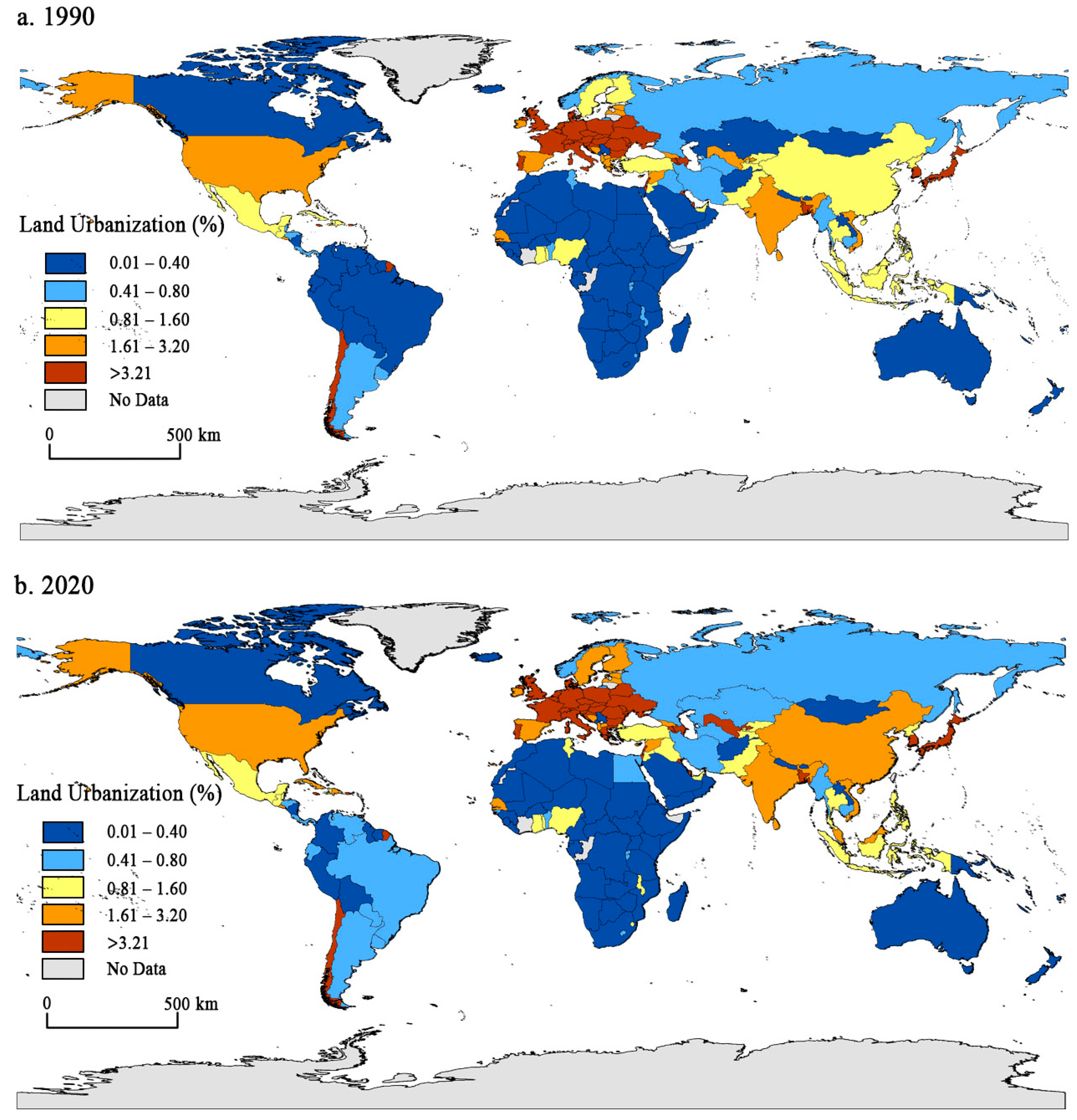
Figure 3 vividly illustrates the spatial distribution dynamics of land urbanization in 1990 and 2020. Throughout the study span, the global spatial pattern of land urbanization exhibited a remarkable degree of stability. High-value zones of land urbanization retained their prominence within Europe, North America, and Southeast Asia. Notably, by 2020, the most robust land urbanization levels were observed in Belgium, Switzerland, Germany, Israel, and Singapore, all strategically positioned within Europe and Asia. Conversely, regions characterized by low land urbanization values encompassed Africa, South America, and Oceania. Remarkably, the five countries showcasing the lowest land urbanization level in 2020 were Mauritania, South Africa, Morocco, Botswana, and Papua New Guinea—all situated in Africa except Papua New Guinea, with their land urbanization figures resting below the 0.01% threshold. This persistent geographical pattern underscores the enduring disparities in land urbanization across different global regions, highlighting the intricate interplay of socioeconomic and environmental factors shaping urbanization dynamics.

3.2. Trends in per Capita CO2 Emissions

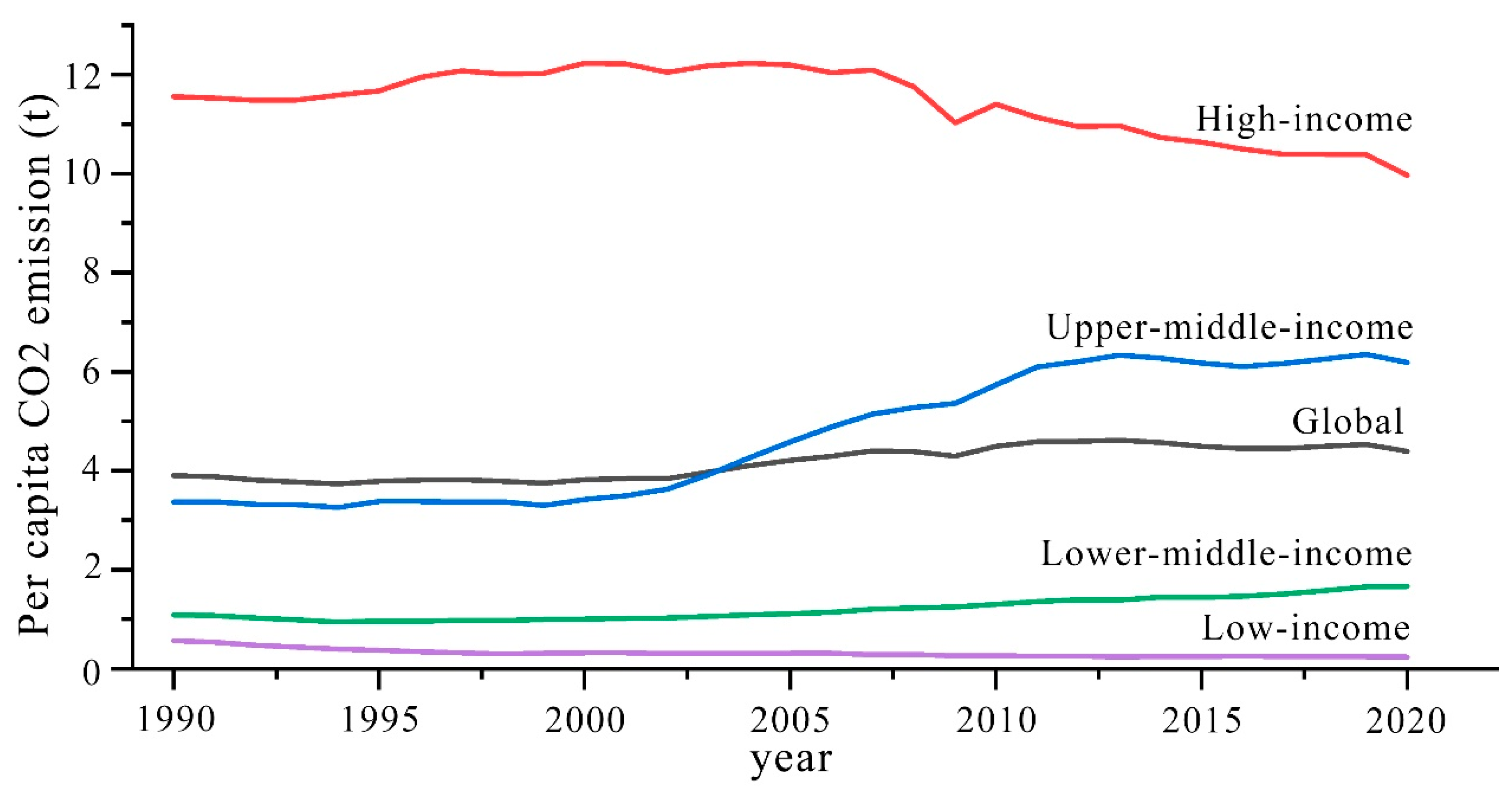
Figure 4 graphically presents the trajectory of per capita CO2 emissions across all panels. As depicted in Figure 4, global per capita CO2 emissions rose from 3.9 t in 1990 to 4.39 t in 2020, indicating a notable 12.5% increase. This upward trend in emissions can be attributed to the persistent expansion of urban construction land worldwide over the last three decades, accompanied by a parallel growth in energy consumption and subsequent carbon emissions. Across each subpanel, the trends in per capita CO2 emissions exhibited diverse patterns during the study period. With reference to existing research [43,44,45], we infer the following reasons for the emergence of each pattern. High-income and low-income countries observed a decline in per capita emissions, which can be linked to their stages of deindustrialization, featuring substantial shifts away from manufacturing that effectively reduced carbon outputs. Simultaneously, technological advancements led to diminished energy intensity, thereby contributing to lower per capita CO2 emissions in these nations. In contrast, upper-middle-income and lower-middle-income countries experienced escalating urbanization and industrialization, precipitating heightened energy demand and subsequently driving an increase in per capita CO2 emissions over the study span. Notably, per capita CO2 emissions in low-income countries also exhibited a decrease over time. This could be attributed to the nascent phase of their industrialization, accompanied by energy consumption growth that lags behind population expansion. Comparing Figure 2 and Figure 4 reveals that the evolutionary trajectories of land urbanization and per capita CO2 emissions exhibit nuanced disparities. However, the incongruence between these trends does not necessarily imply a lack of relationship between land urbanization and per capita CO2 emissions. This study ventures to explore this correlation by introducing the quadratic term of land urbanization to ascertain the potential existence of a nonlinear relationship between these variables.
Similar to land urbanization, per capita CO2 emissions vary significantly between countries at different income levels. With a decrease in income level, per capita CO2 emissions also show a downward trend. Although per capita CO2 emissions in high-income countries declined over the study period, they are still much higher than in other countries. In 2020, for example, the per capita CO2 emissions of high-income countries were 9.96 t, which is 1.6 times, 6.2 times and 42.8 times higher than that of upper-middle-income, lower-middle-income, and low-income countries, respectively.

3.3. Panel Regression Model Results

Prior to conducting panel regression, it becomes imperative to subject the variables to a unit root test in order to ascertain their stationarity. The null hypothesis posits the presence of a unit root within the variable. Should the coefficients of the variables’ intercept and trend demonstrate significance, the null hypothesis is refuted, implying the absence of a unit root. Consequently, the stationarity of the variable can be inferred by assessing the intercept and trend coefficients within the unit root test outcomes. The outcomes of the LLC unit root test and the ADF unit root test are reported in Table 2. A comprehensive analysis of Table 2 highlights that the coefficients of intercept and trend for certain variables do not achieve significance at prescribed levels. This underscores that these specific variables do not display stationarity at those levels. Typically, for variables that do not exhibit stationarity at initial levels, the next step involves applying first differencing to further explore their stationarity [46]. Upon implementing first differencing, the results for the variables reveal that the statistical values derived from both the LLC and ADF tests fall below the critical value set at the 1% threshold (refer to Table 2). As a consequence, all variables nullify the null hypothesis at the 1% significance level, affirming their stationarity following first difference.
Upon achieving first difference stationarity of the variables, the subsequent step involves conducting a cointegration test. The findings of the Pedroni cointegration test are presented in Table 3. Notably, all 11 cointegration statistics within the global panel, as well as those within each individual income subpanel, successfully surpass the threshold for the 1% significance test. This unequivocally rejects the null hypothesis, which posits the absence of any cointegration relationship between the variables. In light of these results, we confidently deduce the existence of a substantive long-term cointegration relationship among the variables under scrutiny.
This study constructs panel regression models to assess the correlation between land urbanization and per capita CO2 emissions across different income samples. The formulated panel regression models are outlined as follows: (1) Model 1 (Global panel); (2) Model 2 (High-income panel); (3) Model 3 (Upper-middle-income panel); (4) Model 4 (Lower-middle-income panel); and (5) Model 5 (Low-income panel). In order to validate the appropriate model form, a Hausman test was conducted, the results of which are presented in Table 4. It is notable that the chi-square statistics associated with all five models surpass the significance level of 1%, consequently rejecting the null hypothesis. This substantiates the adoption of the fixed effects model for executing the subsequent panel regression analysis.
Table 5 reports model regression results for the global panel and each income subpanel. As can be seen in Table 5, there are significant differences in the coefficients of land urbanization and its quadratic terms across panels.
The findings derived from Model 1, as illustrated in Table 5, reveal noteworthy insights. Within the global panel, the LU coefficient emerges as positively significant, while the coefficient of (LU)2 assumes a negative significance, substantiating the existence of an intriguing relationship. Broadly speaking, an “inverted U-shaped” connection is discernible between land urbanization (LU) and per capita CO2 emissions. This relationship signifies that as land urbanization progresses, per capita CO2 emissions initially rise, followed by a subsequent decline. This dynamic can be attributed to the distinct phases of urbanization. During the initial stages of land urbanization, considerable emphasis is placed on infrastructure development, which often leads to heightened energy consumption and, consequently, elevated carbon emissions. As urbanization matures, marked enhancements in urban planning and infrastructure quality materialize, alongside a decrease in energy dependence. Moreover, the growing societal consciousness regarding environmental preservation and carbon mitigation contributes to this shift. These combined factors yield a negative correlation between land urbanization and per capita CO2 emissions during this advanced stage. Furthermore, the model indicates that several factors significantly impact per capita CO2 emissions. Specifically, PGDP (GDP per capita), IS (Industrial Structure), UPD (Urban Population Density), ES (Energy Structure), and EI (Energy Intensity) all exhibit prominent positive effects on per capita CO2 emissions. These findings underscore the intricate interplay between urbanization dynamics, socioeconomic factors, and environmental conditions in shaping the trajectory of per capita CO2 emissions.
The insights derived from Models 2–5, as outlined in Table 5, further elucidate the relationship between land urbanization and per capita CO2 emissions across different income panels. The findings reveal diverse patterns, shedding light on the nuanced dynamics at play in distinct urbanization contexts. High-income countries exhibit an “inverted U-shaped” correlation between land urbanization and per capita CO2 emissions. This suggests that as urbanization progresses, per capita carbon emissions initially increase, only to decrease thereafter. This phenomenon is likely attributed to the advanced urbanization stage of most high-income nations. Recent urban expansion in these countries is often accompanied by heightened emphasis on environmental preservation and green practices. Moreover, technological advancements and shifting societal attitudes have led to reduced energy demands, consequently yielding significant low-carbon effects. Conversely, within lower-middle-income countries, a “U-shaped” association is discernible. As land urbanization advances, per capita CO2 emissions first decline before experiencing an upturn. This trend can potentially be attributed to the relatively lower land use efficiency prevalent in lower-middle-income countries compared to their high-income counterparts. The insufficiency of urban infrastructure during rapid urban expansion in upper-middle-income countries can lead to intensified infrastructure development, which subsequently prompts heightened carbon emissions. Per capita CO2 emissions in low-income countries initially decrease with urbanization before stabilizing. The observed trend implies that while total CO2 emissions may rise in conjunction with urban expansion, per capita CO2 emissions decrease. This outcome is not necessarily indicative of low-carbon and environmentally friendly urban sprawl. Rather, it may signify that carbon emissions in low-income countries are growing at a slower rate than their population size. These intricate variations underscore the multifaceted interplay of economic conditions, urbanization phases, infrastructure development, and population dynamics in shaping the complex relationship between land urbanization and per capita CO2 emissions across different income groups.
Regarding the other variables, noteworthy insights emerge from the panel regression results. In the high-income, upper-middle-income, and lower-middle-income panels, the coefficients associated with PGDP demonstrate a significant positive trend. This signifies that while economic development is not completely disentangled from per capita CO2 emissions, the impact of PGDP on these emissions gradually diminishes as income levels rise. This observation aligns with the notion that advanced economies tend to exhibit a reduced sensitivity of CO2 emissions to economic growth, often attributed to the adoption of more efficient and cleaner technologies. The coefficient of IS yields a significant positive association in both the high-income and upper-middle-income panels. Moreover, this effect is particularly pronounced in high-income countries. This suggests that the industrial structure plays a considerable role in influencing per capita CO2 emissions, with industrial structural changes in high-income nations carrying a stronger influence in comparison to their upper-middle-income counterparts. The influence of UPD on per capita CO2 emissions garners attention across the high-income, upper-middle-income, and lower-middle-income panels, as all exhibit significant effects. In high-income countries, UPD showcases a notable negative impact on per capita CO2 emissions. This can be interpreted as an early reflection of the greening and low-carbon effects of population agglomeration. In contrast, the density of urban populations in upper-middle-income and lower-middle-income countries appears to exert a more complex influence on CO2 emissions, suggesting that the interplay of various factors contributes to these outcomes. The coefficients linked to ES (Energy Structure) and EI (Energy Intensity) emerge as significantly positive in the high-income, upper-middle-income, and lower-middle-income panels. This implies that energy consumption remains intertwined with per capita CO2 emissions across these income strata, highlighting that efforts to decouple energy consumption from emissions have not been fully realized in these contexts. These multifaceted outcomes emphasize the intricate interplay between economic development, industrial structure, population dynamics, and energy-related factors in shaping the relationships between per capita CO2 emissions and various influencing variables across different income groups.

4. Conclusions and Discussion

This study comprehensively examines the evolutionary trends of land urbanization and per capita CO2 emissions across a global dataset encompassing 195 countries. Through the utilization of panel regression models, the research delves into the carbon emission implications of land urbanization across different income samples. Moreover, the study employs the EKC theory to dissect the potential nonlinear relationship between land urbanization and per capita CO2 emissions. The investigation unveils a consistent growth trend in both land urbanization and per capita CO2 emissions from 1990 to 2020. Notably, significant disparities in land urbanization and per capita carbon emissions are evident among nations at varying income levels. A discernible trend emerges wherein land urbanization and per capita CO2 emissions exhibit a decreasing trajectory as income levels diminish. The outcomes of the panel regression analyses underscore the intricate nature of this relationship across different income panels. The study yields intriguing insights: an “inverted U-shaped” correlation surfaces between land urbanization and per capita CO2 emissions within the global and high-income panels, while a “U-shaped” association characterizes the relationship in lower-middle-income countries. Upper-middle-income and low-income countries, in contrast, demonstrate a more straightforward linear relationship between land urbanization and per capita CO2 emissions. This research not only provides a comprehensive perspective on the evolution of land urbanization and its carbon emissions implications, but also elucidates the nuanced interplay between these dynamics within diverse economic contexts. By incorporating the EKC theory, the study contributes to a deeper understanding of the nonlinear facets shaping the intricate linkage between land urbanization and per capita CO2 emissions.
A comparative analysis of the urbanization trajectories across diverse countries underscores a prevailing trend: the initial stages of land urbanization often exhibit suboptimal quality. Early urban sprawl, driven by the imperatives of socioeconomic advancement, tends to demand significant energy resources. However, as socioeconomic development matures, the convergence of technological advancements and heightened environmental awareness leads to a more efficient and environmentally conscious approach to urban expansion [47].
The growing asymmetry in developmental trajectories among global nations is becoming increasingly conspicuous. The implications of this study’s findings underscore the imperative for future carbon reduction policies to account for national development levels. Moreover, countries should tailor their land urbanization strategies to their unique national contexts. High-income countries, given their disproportionately high per capita CO2 emissions, are urged to intensify their efforts to curtail carbon emissions. This entails a concerted focus on reshaping industrial and energy structures, without the sole focus on endless economic growth, in order to reduce per capita carbon emissions. For upper-middle-income and lower-middle-income countries, adopting a sustainable approach to land urbanization emerges as a viable strategy. Drawing insights from the expansion patterns of high-income countries, emphasis should be placed on the quality of land urbanization. Specifically, the focus is on preserving urban environments, promoting sustainable urban development, and increasing urban land efficiency. This entails mitigating the ecological pressures resulting from urban expansion, and aligning such expansion with the capacity of local resources and the environment. For low-income countries, developmental aspirations assume paramount significance. With a focus on achieving comprehensive development, enhancing the quality of land urbanization becomes a crucial objective. By ensuring that development occurs in a manner that respects ecological thresholds, these countries can foster an environment where urban expansion aligns harmoniously with the available resources and environmental capacities.
In conclusion, this study underscores the critical need for tailored and context-specific land urbanization strategies. By aligning such strategies with socioeconomic development levels, nations can navigate the intricate interplay between urbanization, carbon emissions, and sustainable growth, thereby contributing to a more balanced and environmentally conscious global development landscape.
The results of this study suggest that countries should not ignore their own stage of development when making carbon reduction policies. The findings deepen our understanding of the carbon emission effect of land urbanization in countries at different development stages, and also provide policy references for countries to choose land urbanization strategies. As a transnational study on carbon emissions, this study also has a limitation. Specifically, it does not account for the influence of international trade between countries. Considering that countries are increasingly interconnected, factors such as resources and environment will flow across borders under the influence of trade. Therefore, future extensions of the work can focus on the carbon emission effects of urbanization from the perspective of the consumption side. Furthermore, it is necessary to further explore whether the carbon emission effect of urbanization is short-term or long-term, which is crucial for governments to formulate carbon reduction policies.

Author Contributions

Methodology, Y.X.; Investigation, S.W.; Writing—original draft, Y.X., Y.L., Z.L. (Zhe Li), Z.L. (Zhuojun Li) and S.W.; Supervision, S.W. All authors have read and agreed to the published version of the manuscript.

Funding

This work was supported by Guangdong Enterprise Key Laboratory for Urban Sensing, Monitoring and Early Warning (No.2020B121202019), The Science and Technology Foundation of Guangzhou Urban Planning & Design Survey Research Institute (No. RDI2210202016; No. RDI2220202098) and the Guangzhou Social Science Planning Project (No.2023GZYB81).

Data Availability Statement

The data are contained within the article.

Conflicts of Interest

The authors declare no conflict of interest.

References

  1. Chen, M.; Huang, Y.; Tang, Z.; Lu, D.; Liu, H.; Ma, L. The provincial pattern of the relationship between urbanization and economic development in China. J. Geogr. Sci. 2014, 24, 33–45. [Google Scholar] [CrossRef]
  2. OECD. Cities in the World: A New Perspective on Urbanisation; OECD Urban Studies/European Union: Paris, France, 2020. [Google Scholar]
  3. Romano, B.; Zullo, F. Land urbanization in Central Italy: 50 years of evolution. J. Land Use Sci. 2014, 9, 143–164. [Google Scholar] [CrossRef]
  4. Liu, X.; Huang, Y.; Xu, X.; Li, X.; Li, X.; Ciais, P.; Lin, P.; Gong, K.; Ziegler, A.D.; Chen, A. High-spatiotemporal-resolution mapping of global urban change from 1985 to 2015. Nat. Sustain. 2020, 3, 564–570. [Google Scholar] [CrossRef]
  5. Feng, W.; Liu, Y.; Qu, L. Effect of land-centered urbanization on rural development: A regional analysis in China. Land Use Policy 2019, 87, 104072. [Google Scholar] [CrossRef]
  6. Díaz-Pacheco, J.; García-Palomares, J.C. Urban sprawl in the Mediterranean urban regions in Europe and the crisis effect on the urban land development: Madrid as study case. Urban Stud. Res. 2014, 2014, 807381. [Google Scholar] [CrossRef]
  7. Long, H.; Zhang, Y.; Ma, L.; Tu, S. Land use transitions: Progress, challenges and prospects. Land 2021, 10, 903. [Google Scholar] [CrossRef]
  8. Jiang, L.; O’Neill, B.C. Global urbanization projections for the Shared Socioeconomic Pathways. Glob. Environ. Chang. 2017, 42, 193–199. [Google Scholar] [CrossRef]
  9. Ye, F.; Wang, W. Determinants of Land Finance in China: A Study Based on Provincial-level Panel Data. Aust. J. Public Adm. 2013, 72, 293–303. [Google Scholar]
  10. Cao, G.; Feng, C.; Tao, R. Local “land finance” in China’s urban expansion: Challenges and solutions. China World Econ. 2008, 16, 19–30. [Google Scholar] [CrossRef]
  11. Zhang, T. Land market forces and government’s role in sprawl: The case of China. Cities 2000, 17, 123–135. [Google Scholar] [CrossRef]
  12. Tong, D.; Chu, J.; Han, Q.; Liu, X. How land finance drives urban expansion under fiscal pressure: Evidence from Chinese cities. Land 2022, 11, 253. [Google Scholar] [CrossRef]
  13. Lin, X.; Wang, Y.; Wang, S.; Wang, D. Spatial differences and driving forces of land urbanization in China. J. Geogr. Sci. 2015, 25, 545–558. [Google Scholar] [CrossRef]
  14. Bai, X.; Chen, J.; Shi, P. Landscape urbanization and economic growth in China: Positive feedbacks and sustainability dilemmas. Environ. Sci. Technol. 2012, 46, 132–139. [Google Scholar] [CrossRef] [PubMed]
  15. Tian, Y.; Tsendbazar, N.-E.; van Leeuwen, E.; Fensholt, R.; Herold, M. A global analysis of multifaceted urbanization patterns using Earth Observation data from 1975 to 2015. Landsc. Urban Plan. 2022, 219, 104316. [Google Scholar] [CrossRef]
  16. Cao, S.; Lv, Y.; Zheng, H.; Wang, X. Challenges facing China’s unbalanced urbanization strategy. Land Use Policy 2014, 39, 412–415. [Google Scholar] [CrossRef]
  17. Chen, M.; Liu, W.; Lu, D. Challenges and the way forward in China’s new-type urbanization. Land Use Policy 2016, 55, 334–339. [Google Scholar] [CrossRef]
  18. He, C.; Zhou, Y.; Huang, Z. Fiscal decentralization, political centralization, and land urbanization in China. Urban Geogr. 2016, 37, 436–457. [Google Scholar] [CrossRef]
  19. Liu, X.; Xin, L. Assessment of the efficiency of cultivated land occupied by urban and rural construction land in China from 1990 to 2020. Land 2022, 11, 941. [Google Scholar] [CrossRef]
  20. Wang, Y.; Li, L.; Kubota, J.; Han, R.; Zhu, X.; Lu, G. Does urbanization lead to more carbon emission? Evidence from a panel of BRICS countries. Appl. Energy 2016, 168, 375–380. [Google Scholar] [CrossRef]
  21. Wang, S.; Fang, C.; Ma, H.; Wang, Y.; Qin, J. Spatial differences and multi-mechanism of carbon footprint based on GWR model in provincial China. J. Geogr. Sci. 2014, 24, 612–630. [Google Scholar] [CrossRef]
  22. Fan, J.-L.; Zhang, Y.-J.; Wang, B. The impact of urbanization on residential energy consumption in China: An aggregated and disaggregated analysis. Renew. Sustain. Energy Rev. 2017, 75, 220–233. [Google Scholar] [CrossRef]
  23. Zhou, C.; Wang, S.; Wang, J. Examining the influences of urbanization on carbon dioxide emissions in the Yangtze River Delta, China: Kuznets curve relationship. Sci. Total Environ. 2019, 675, 472–482. [Google Scholar] [CrossRef] [PubMed]
  24. Hossain, M.S. Panel estimation for CO2 emissions, energy consumption, economic growth, trade openness and urbanization of newly industrialized countries. Energy Policy 2011, 39, 6991–6999. [Google Scholar] [CrossRef]
  25. Wang, Z.; Cui, C.; Peng, S. How do urbanization and consumption patterns affect carbon emissions in China? A decomposition analysis. J. Clean. Prod. 2019, 211, 1201–1208. [Google Scholar] [CrossRef]
  26. Sharma, S.S. Determinants of carbon dioxide emissions: Empirical evidence from 69 countries. Appl. Energy 2011, 88, 376–382. [Google Scholar] [CrossRef]
  27. Khansari, N.; Mostashari, A.; Mansouri, M. Conceptual modeling of the impact of smart cities on household energy consumption. Procedia Comput. Sci. 2014, 28, 81–86. [Google Scholar] [CrossRef]
  28. Zhu, H.-M.; You, W.-H.; Zeng, Z.-F. Urbanization and CO2 emissions: A semi-parametric panel data analysis. Econ. Lett. 2012, 117, 848–850. [Google Scholar] [CrossRef]
  29. Zhang, Y.; Wu, Q.; Fath, B.D. Review of spatial analysis of urban carbon metabolism. Ecol. Model. 2018, 371, 18–24. [Google Scholar] [CrossRef]
  30. Zhang, N.; Yu, K.; Chen, Z. How does urbanization affect carbon dioxide emissions? A cross-country panel data analysis. Energy Policy 2017, 107, 678–687. [Google Scholar] [CrossRef]
  31. Al-Mulali, U.; Sab, C.N.B.C.; Fereidouni, H.G. Exploring the bi-directional long run relationship between urbanization, energy consumption, and carbon dioxide emission. Energy 2012, 46, 156–167. [Google Scholar] [CrossRef]
  32. Wang, S.; Gao, S.; Li, S.; Feng, K. Strategizing the relation between urbanization and air pollution: Empirical evidence from global countries. J. Clean. Prod. 2020, 243, 118615. [Google Scholar] [CrossRef]
  33. Dickey, D.A.; Fuller, W.A. Distribution of the estimators for autoregressive time series with a unit root. J. Am. Stat. Assoc. 1979, 74, 427–431. [Google Scholar]
  34. Dickey, D.A.; Fuller, W.A. Likelihood ratio statistics for autoregressive time series with a unit root. Econom. J. Econom. Soc. 1981, 49, 1057–1072. [Google Scholar] [CrossRef]
  35. Al-Mulali, U.; Fereidouni, H.G.; Lee, J.Y.; Sab, C.N.B.C. Exploring the relationship between urbanization, energy consumption, and CO2 emission in MENA countries. Renew. Sustain. Energy Rev. 2013, 23, 107–112. [Google Scholar] [CrossRef]
  36. Ou, J.; Liu, X.; Li, X.; Chen, Y. Quantifying the relationship between urban forms and carbon emissions using panel data analysis. Landsc. Ecol. 2013, 28, 1889–1907. [Google Scholar] [CrossRef]
  37. Engle, R.F.; Granger, C.W. Co-integration and error correction: Representation, estimation, and testing. Econom. J. Econom. Soc. 1987, 55, 251–276. [Google Scholar] [CrossRef]
  38. Pedroni, P. Purchasing power parity tests in cointegrated panels. Rev. Econ. Stat. 2001, 83, 727–731. [Google Scholar] [CrossRef]
  39. Xu, B.; Lin, B. How industrialization and urbanization process impacts on CO2 emissions in China: Evidence from nonparametric additive regression models. Energy Econ. 2015, 48, 188–202. [Google Scholar] [CrossRef]
  40. Wang, S.; Li, Q.; Fang, C.; Zhou, C. The relationship between economic growth, energy consumption, and CO2 emissions: Empirical evidence from China. Sci. Total Environ. 2016, 542, 360–371. [Google Scholar] [CrossRef]
  41. Wang, S.; Fang, C.; Guan, X.; Pang, B.; Ma, H. Urbanisation, energy consumption, and carbon dioxide emissions in China: A panel data analysis of China’s provinces. Appl. Energy 2014, 136, 738–749. [Google Scholar] [CrossRef]
  42. Grossman, G.M.; Krueger, A.B. Economic growth and the environment. Q. J. Econ. 1995, 110, 353–377. [Google Scholar] [CrossRef]
  43. Liu, Q.; Wang, S.; Zhang, W.; Li, J.; Kong, Y. Examining the effects of income inequality on CO2 emissions: Evidence from non-spatial and spatial perspectives. Appl. Energy 2019, 236, 163–171. [Google Scholar] [CrossRef]
  44. Wang, J.; Wang, S.; Zhou, C.; Feng, K. Consumption-based carbon intensity of human well-being and its socioeconomic drivers in countries globally. J. Clean. Prod. 2022, 366, 132886. [Google Scholar] [CrossRef]
  45. Hao, Y. Effect of economic indicators, renewable energy consumption and human development on climate change: An empirical analysis based on panel data of selected countries. Front. Energy Res. 2022, 10, 841497. [Google Scholar] [CrossRef]
  46. Zhao, Y.; Wang, S. The relationship between urbanization, economic growth and energy consumption in China: An econometric perspective analysis. Sustainability 2015, 7, 5609–5627. [Google Scholar] [CrossRef]
  47. Poumanyvong, P.; Kaneko, S. Does urbanization lead to less energy use and lower CO2 emissions? A cross-country analysis. Ecol. Econ. 2010, 70, 434–444. [Google Scholar] [CrossRef]
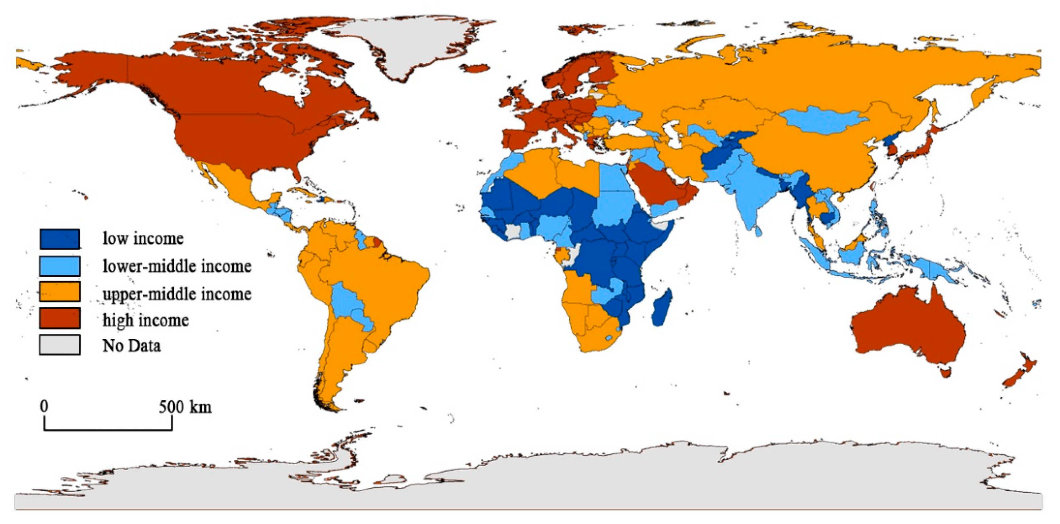
Figure 1. The spatial distribution of the income levels of countries, 2015.
Land 12 01930 g001
Figure 2. Evolution trend of land urbanization level in countries from 1990 to 2020.
Land 12 01930 g002
Figure 3. Spatial distribution pattern of land urbanization in 1990 and 2020.
Land 12 01930 g003
Figure 4. Evolution trend of per capita CO2 emissions in countries from 1990 to 2020.
Land 12 01930 g004
Table 1. Variables and descriptive statistics.
VariablesDefinitionUnitObsMeanRangeStd.Dev
PCO2Per capita CO2 emissiont60454.3747.695.46
LULand urbanization (Urban built-up area/total area)%60452.59.633.08
PGDPPer capita GDPconstant dollar604511,41944,00614,074
ISIndustrial structure (Industrial added value/GDP)%604526.5282.3912.42
UPDUrban population densitypersons/km26045199113,5052917
ESEnergy structure (Share of fossil fuel energy consumption)%604572.6710028.58
EIEnergy intensity (Energy consumption/GDP)tce/104 constant dollar604512.0176.5310.56
Table 2. Panel unit root test results.
VariableLevelFirst Difference
InterceptIntercept and TrendInterceptIntercept and Trend
Levin-Lin-Chu test (common root)
PCO22.709−8.964−49.944 ***−45.427 ***
LU30.693−3.671 ***−49.236 ***−49.102 ***
PGDP21.347−2.317 *−32.991 ***−31.458 ***
IS−3.948 ***2.232−46.085 ***−35.827 ***
UPD25.931−0.007 *−12.897 ***−19.121 ***
ES18.95319.532−34.043 ***−27.999 ***
EI−3.911 ***−0.545−53.209 ***−45.787 ***
ADF-Fisher Chi-square test (individual root)
PCO2562.816 ***823.652 ***3128.17 ***2983.16 ***
LU33.8561026.11 ***3610.91 ***6695.84 ***
PGDP299.042712.372 ***2013.36 ***1892.04 ***
IS576.408 ***530.664 ***2996.83 ***2635.1 ***
UPD419.742 *370.3681042.97 ***1295.57 ***
ES342.296315.9842469.38 ***2199.02 ***
EI429.569 **523.523 ***3302.48 ***2935.05 ***
Note: *, ** and *** indicate significance at the 10% level, 5% level, and 1% level.
Table 3. Cointegration test results.
GlobalHigh-Upper-
Middle-
Lower-
Middle-
Low-
Alternative hypothesis: common AR coefs. (within-dimension)
Panel v-Statistic−5.537 ***−2.716 ***−4.145 ***−3.640 ***−2.077 ***
Panel rho-Statistic6.181 ***3.047 ***3.841 ***4.249 ***4.473 ***
Panel PP-Statistic5.602 ***2.431 ***3.678 ***5.279 ***6.966 ***
Panel ADF-Statistic5.637 ***2.571 ***4.827 ***5.621 ***2.516 ***
Panel v-Statistic (weighted)−6.062 **−2.478 ***−3.854 ***−3.511 ***−1.724 ***
Panel rho-Statistic (weighted)6.575 ***2.201 ***3.513 ***4.678 ***2.304 ***
Panel PP-Statistic (weighted)6.731 ***1.206 ***3.466 ***5.091 ***2.501 ***
Panel ADF-Statistic (weighted)6.868 ***0.029 ***4.369 ***5.989 **3.074 ***
Alternative hypothesis: individual AR coefs. (between-dimension)
Group rho-Statistic8.209 ***3.641 ***4.426 ***5.258 ***2.945 ***
Group PP-Statistic8.184 ***1.671 ***4.389 ***7.208 ***3.082 ***
Group ADF-Statistic8.431 ***0.101 ***5.871 ***7.511 ***3.501 ***
Note: ** and *** indicate significance at the 5% level, and 1% level.
Table 4. Hausman test results.
Chi-Sq Statisticp ValuesType of Regression Model
Model 118.880.0044Fixed effects
Model 232.280.0000Fixed effects
Model 327.810.0001Fixed effects
Model 4102.510.0000Fixed effects
Model 5553.560.0000Fixed effects
Table 5. Panel regression results.
VariablesModel 1Model 2Model 3Model 4Model 5
lnLU0.445 ***
(0.081)
0.776 ***
(0.120)
0.095 ***
(0.151)
−1.527 ***
(0.181)
−1.000 **
(0.459)
(lnLU)2−0.047 ***
(0.015)
−0.042 *
(0.024)
0.007
(0.035)
0.234 ***
(0.026)
−0.018
(0.069)
lnPGDP0.459 ***
(0.013)
0.374 ***
(0.031)
0.582 ***
(0022)
0.808 ***
(0.027)
−0.136 ***
(0.037)
lnIS0.115 ***
(0.016)
0.240 ***
(0.032)
0.108 ***
(0.035)
0.034
(0.028)
−0.001
(0.034)
lnUPD0.123 ***
(0.019)
−0.084 ***
(0.029)
0.134 ***
(0.044)
0.266 ***
(0.032)
0.613
(0.076)
lnES0.549 ***
(0.018)
0.353 ***
(0.041)
0.603 ***
(0.059)
0.461 ***
(0.029)
0.654
(0.033)
lnEI0.446 ***
(0.011)
0.155 ***
(0.022)
0.397 ***
(0.021)
0.326 ***
(0.018)
0.322
(0.029)
Constant−7.569 ***
(0.206)
−5.625 ***
(0.444)
−8.023 ***
(0.452)
−11.254 ***
(0.402)
−10.086 ***
(1.224)
R-squared0.5310.3210.5430.7470.615
F-statistic235.95524.85106.03139.93110.73
p value0.0000.0000.0000.0000.000
Obs5837182915971505906
Note: *, ** and *** indicate significance at the 10% level, 5% level, and 1% level.
Disclaimer/Publisher’s Note: The statements, opinions and data contained in all publications are solely those of the individual author(s) and contributor(s) and not of MDPI and/or the editor(s). MDPI and/or the editor(s) disclaim responsibility for any injury to people or property resulting from any ideas, methods, instructions or products referred to in the content.