Article

GIS-Based RUSLE Reservoir Sedimentation Estimates: Temporally Variable C-Factors, Sediment Delivery Ratio, and Adjustment for Stream Channel and Bank Sediment Sources

by
Patrick J. Starks
*,
Daniel N. Moriasi
and
Ann-Marie Fortuna
Agroclimate and Hydraulic Engineering Research Unit, United States Department of Agriculture, Agricultural Research Service, Oklahoma and Central Plains Agricultral Research Center, 7207 W. Cheyenne St., El Reno, OK 73036, USA
*
Author to whom correspondence should be addressed.
Land 2023, 12(10), 1913; https://doi.org/10.3390/land12101913
Submission received: 22 August 2023 / Revised: 22 September 2023 / Accepted: 3 October 2023 / Published: 12 October 2023
(This article belongs to the Section Soil-Sediment-Water Systems)

Abstract

:
The empirical Revised Universal Soil Loss Equation (RUSLE) has been adapted to geographical information system (GIS) frameworks to study the spatial variability of soil erosion across landscapes and has also been used to estimate reservoir sedimentation. The literature presents contradictory results about the efficacy of using RUSLE in a GIS context for quantifying reservoir sedimentation, requiring further evaluation and validation of its estimates relative to measured reservoir sedimentation. Our primary objective was to determine if these contradictory results may be a function of the RUSLE’s inability to account for sediments derived from gullies, stream channels, or stream banks; the temporal variability of some of RUSLE’s empirically based factors such as the land cover/land management (C-) factor; and in some model renditions, the choice of value for the sediment delivery ratio (SDR). The usefulness of adjusting these estimates using a regional representative value of gully/stream bank sediment contributions was also assessed. High-spatial horizontal resolution (2 m) digital elevation models (DEMs) for 12 watersheds were used together with C-factor data for five representative years in a GIS-based RUSLE model that incorporates SDR within a sediment routing routine to study the impacts of choice of C-factor and SDR on reservoir sedimentation estimates. Choice of image date for developing C-factors was found to impact reservoir estimates. We also found that the value of SDR for some of the study watersheds would have to be unrealistically small to produce sedimentation estimates comparable to measured values. Estimates of reservoir sedimentation were comparable to measured data for 5 of the 12 watersheds, when the regionally based adjustment for gully/stream bank contributions was applied. However, differences remained large for the remaining seven watersheds. Statistical analysis revealed that certain combinations of geomorphic, pedologic, or topographic variables could be used to predict the degree of sediment underestimation with a significant and high level of correlation (0.72 < R2 ≤ 0.99; p-value < 0.05). Our findings indicate that the level of agreement between GIS-based RUSLE estimates of reservoir sedimentation and measured values is a function of watershed characteristics; for example, the area-weighted soil erodibility (K-) factor of the soils within the watershed and stream channels, the stream entrenchment ratio and bank full depth, the percentage of the stream corridor having slopes ≥ 21°, and the width of the stream flood way as a percentage of the watershed area. Within the context of GIS, these metrics are easily obtained from digital elevation models and publicly available soils data and may be useful in prioritizing reservoirs’ assessments for function and safety.

1. Introduction

During the 1930s, severe drought and poor conservation practices in Oklahoma and the Southern Great Plains resulted in decreased vegetative cover, which combined with subsequent periods of intense rainfall caused increased erosion and flooding [1]. Because of these natural disasters, the U.S. Congress passed the Flood Control Act of 1944 (PL-534) and the Watershed Protection and Flood Prevention Act of 1954 (PL-566) to minimize soil erosion and to prevent flooding [2,3]. As a result of these Acts, the Washita River Basin (WRB) in Oklahoma was 1 of 11 pilot watershed projects selected for the construction of flood control reservoirs. Through the PL-534 and PL-566 projects, the United States Department of Agriculture (USDA) Natural Resources Conservation Service in Oklahoma provided technical and financial assistance for the construction of 2107 flood control dams (~20% of the national total) [1]. Forty-five of these dams were built in the Little Washita River Watershed (LWREW, located in the WRB) between 1969 and 1982 [4].
Bennett et al. [5] projected that by 2020 about 50% of the USDA Natural Resources Conservation Service (NRCS) reservoirs would be near the end of their projected 50-year service life due to sedimentation. Reduction in reservoir sediment trapping can lead to reduced usable pool depth and flood storage capacity and decreased future sediment storage, projected lifespan, and agricultural productivity [6]. For these reasons, these reservoirs need to be evaluated for rehabilitation or decommissioning [7].
Due to aging of these NRCS structures, Section 313 of Public Law 106–472 [8] provided authorization to conduct an evaluation of the reservoirs for possible extension of service life of the structures, for conformance to applicable safety and performance standards, or for decommissioning. A common first step in the assessment for rehabilitation is to survey the amount of sediment in the reservoir [6]. Often, such assessments require labor intensive and costly measures to conduct, for example, acoustic profiling and sediment coring, which would become more prohibitive if trying to assess sedimentation for many reservoirs. Modeling is a good choice for conducting preliminary assessments, especially in the context of prioritizing watersheds for follow-up investigations. However, process-based models such as Water Erosion Prediction Project (WEPP) [9] and European Soil Erosion Model (EUROSEM) [10] often require data that may not be available or are difficult to acquire [11]; thus, empirical models such as the Revised Universal Soil Loss Equation (RUSLE) [12] are often used. RUSLE is an improvement upon its USLE predecessor [13], an empirical equation developed from >10,000 plot-years of soil erosion and runoff data [13] and originally intended for field-based applications. The RUSLE requires five inputs to calculate soil loss: a rainfall and runoff factor (R), a soil erodibility factor (K), a slope length and steepness factor (LS), a land cover and management factor (C), and a support practice factor (P). Due to increased computing power over the last several decades and the development of geographical information systems (GIS), RUSLE has been increasingly used for spatial analysis of soil erosion for landscapes and watersheds of various sizes [14,15,16].
The review of the literature indicates that many GIS-based RUSLE soil erosion studies focused on temporal erosion trends and the assessment of relative changes in sediment production [17] and for targeting erosion “hot spots” within watersheds [18]. There are a limited number of RUSLE-based studies that have been conducted wherein the spatial distribution of plant, soil, land management, rainfall, and topographic variables were used to estimate reservoir sedimentation for comparison against measured reservoir sediment accumulation [19,20,21,22]. However, the literature presents contradictory results for the efficacy of using RUSLE in a GIS context for quantifying reservoir sedimentation. Boomer et al. [19] applied the USLE and RUSLE2 (second generation of RUSLE) to 78 small sub-watersheds within the Chesapeake Bay watershed and reported that the USLE family of models exceeded measured annual average sediment delivery by more than 100%. Moges et al. [20] reported that GIS-based RUSLE estimates were ~1.3, and 1.7 times larger than those measured for the Selamko and Shina watersheds, respectively, in the Ethiopian Blue Nile basin. Kaffas et al. [12] also used a spatially distributed version of RUSLE to estimate reservoir sedimentation for the Rio di Pusteria reservoir in the Italian Alps. In that study, the researchers used two different methods to calculate the RUSLE R-factor, i.e., one representing the 5 yr study period, and the second representing the long-term average conditions. Kaffas et al. [21] also adjusted the initial RUSLE estimates via a sediment delivery ratio (SDR) and found that estimated reservoir sedimentation was within 3.1% and −23.2%, depending upon R-factor method used, and was within 12.5% of the measured value if the SDR adjustment was used. Bufalini et al. [22] compared bathymetric sediment measurements of a reservoir in central Italy, and estimated via a GIS-based RUSLE. In their study, Bufalini et al. [22] calculated the P-factor in three separate ways, which had a profound effect on the RUSLE sediment estimates. These researchers concluded that a GIS-based RUSLE approach could be used to reasonably estimate reservoir sedimentation if the RUSLE parameters were properly calibrated.
Multiple authors have noted that the main weakness of the RUSLE model is that it does not account for gully erosion, stream bank instabilities, and channel contributions to the sediment load [15,19,20,21,23,24,25]. Simon and Rinaldi [26] showed that stream bank erosion accounted for 64 to 90% of the total sediment load for four streams in the Southeastern U.S. Wilson et al. [27] showed, using ratios of 7Be to 210Pb, that eroded surface soils in the Fort Cobb Reservoir watershed (located in Southwestern Oklahoma) only accounted for 46% of suspended sediments in streams following a runoff event. Simon and Klimetz [28] noted that ~60% of the stream channels in the LWREW—our study area—are unstable and contribute a considerable amount of sediment to downstream reservoirs. Other weaknesses of the RUSLE approach were outlined by Benavidez et al. [29] and included choice of spatial resolution of the digital elevation models (DEMs) used in the study (which affects the calculation of the LS factor), granularity and scale of land cover characteristics, and choice of values for the RUSLE factors. These authors added that another limitation of the RUSLE approach is the lack of validation data to verify the model’s output. Therefore, there is a need for further evaluation and validation of the GIS-based RUSLE approach to estimate reservoir sedimentation, specifically regarding the impact of temporally variable land cover data sets and the impact of channel and stream bank contributions to reservoir sedimentation. It may be possible to improve the usefulness of a GIS-based RUSLE approach through evaluation of linkages between measured reservoir sedimentation and easily obtainable geomorphic, pedologic, and topographic metrics.
Our objectives are as follows: (1) quantify the impact of temporally variable C-factors on the estimation of long-term average reservoir sedimentation, (2) determine if a regionally based adjustment, suggested by the results of Wilson et al. [27], can be used as a first-order correction to account for sediment contributions from gullies, stream channels, and stream banks, and (3) examine linkages between estimated reservoir sedimentation and watershed, stream, stream corridor, and stream bank variables acquired from high-spatial horizontal resolution (2 m) digital elevation models (DEMs), satellite-based land cover data sets, and publicly available soils data.

2. Material and Methods
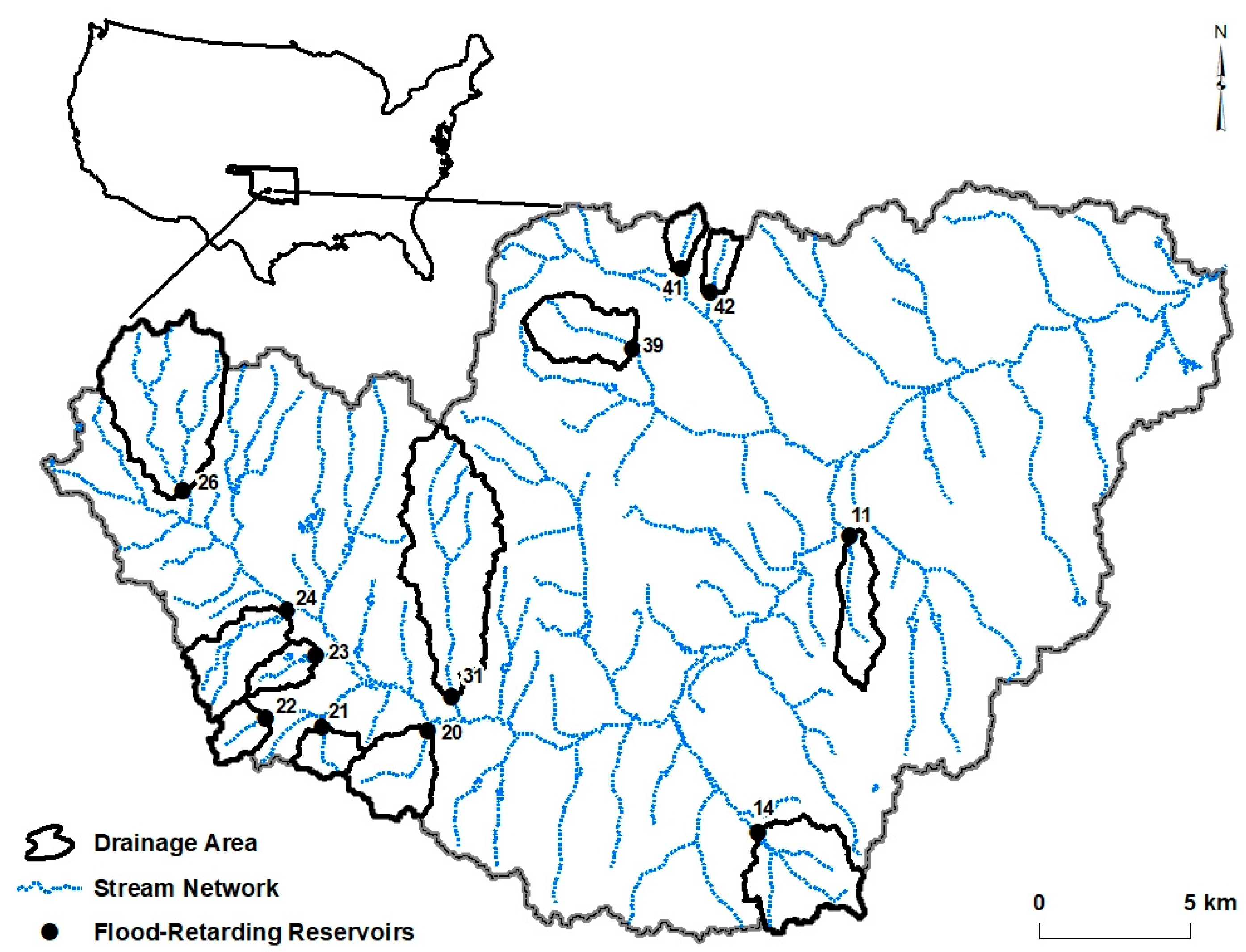
2.1. Study Sites

2.1.1. General Description

The study was conducted on 12 watersheds and their accompanying reservoirs located in the LWREW, in Southwestern Oklahoma, USA [1] (Figure 1). The LWREW is ~610 km2 in size and is characterized by gently to moderately rolling topography with a maximum relief of 490 m [4]. The soils in the central section of the LWREW are sandy in texture, whereas silty loam and loamy soils are found in the western and eastern sections. The 1991–2020 normal annual precipitation was ~807 mm, with about 27 and 20% of the annual total precipitation occurring in the months of May–June and September–October, respectively. The annual average daily temperature is 15.6 °C, with annual maximum and minimum air temperatures occurring in July (27.9 °C) and January (3.2 °C), respectively [30].
The reservoirs evaluated in this study were impounded between 1969 and 1982 (Table 1) and are further described by Moriasi et al. [1]. The watershed drainage areas, reservoir surface areas, and principal land uses [4] are provided in Table 1. The dominant land cover within each watershed is grassland, which varies between watersheds, ranging from 44 to 80%. In four of the twelve watersheds, 21 to 44% of their areas are tree/shrub lands, and in another four, 15 to 43% of their areas are cropped areas. These subdominant land cover categories (Table 1) were used in the statistical analysis to identify possible differences in reservoir sedimentation due to land cover factors.
Moriasi et al. [1] conducted a bathymetric survey of the twelve reservoirs during 14–25 May 2012 using a multifrequency acoustic profiling system. The details of this survey and the device used to collect the data are provided by Moriasi et al. [1]. The impoundment period (representing the time from impoundment to the survey date) varied from 29.6 yr (Reservoir 20) to 42.6 yr (Reservoir 42) (Table 1). The measured reservoir sediment volumes ranged from 24,155 to 439,581 m3 (Table 1).
Figure 1. Location and identification numbers of the study watersheds within the LWREW.
Land 12 01913 g001

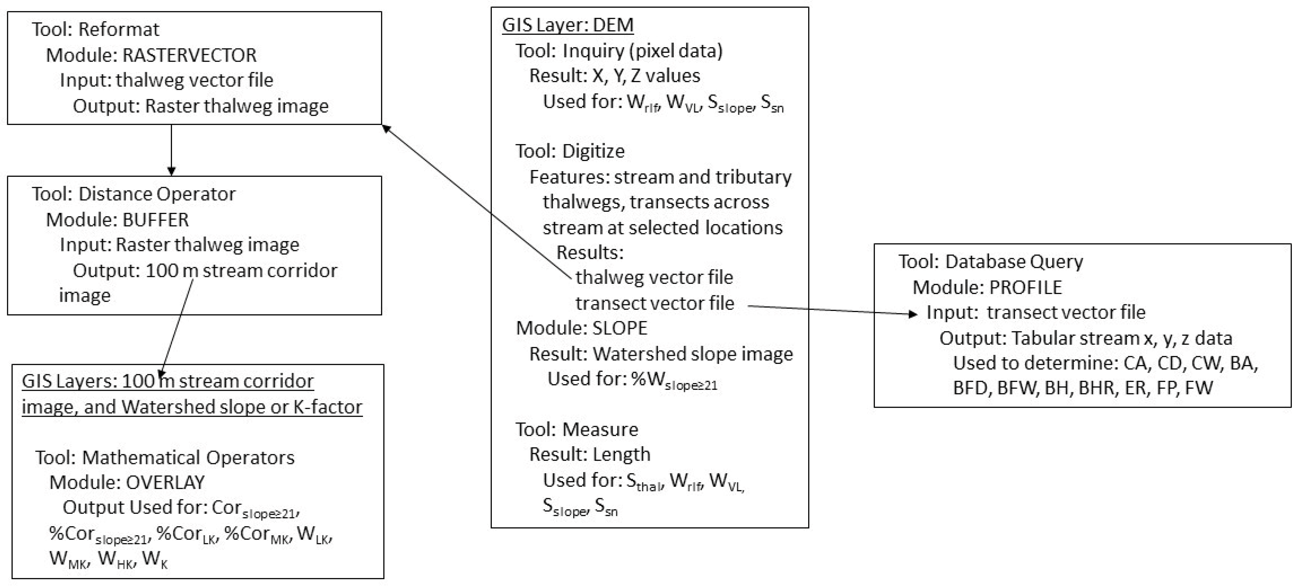
2.1.2. Watershed and Stream Geomorphic and Topographic Variables

In addition to the data required to run the RUSLE model, several variables were identified or developed (Figure 2) and measured to assist in interpreting differences between measured and estimated reservoir sedimentation. These variables include percentage of watershed area having slopes ≥ 21° (%Wslope ≥ 21), watershed basin relief (Wrlf), watershed valley length (Wvl), stream slope (Sslope), stream thalweg length (Sthal), and stream sinuosity (Ssn).
Watershed slope images were created within the Idrisi TerrSet 2020 (Clarke Labs, Clarke University, Clarke, MA, USA) GIS software, and the pixel-based values were downloaded for statistical evaluation. The %Wslope ≥ 21 was developed based on the findings of [1], which indicated that the land area with slopes ≥ 21° was a useful metric to quantify topographic effects on reservoir sedimentation. Slope images for each watershed are shown in Supplemental Figures S1–S12. Basin relief was calculated as the difference between the highest and lowest (outlet) elevations in the watershed. Stream thalwegs were digitized from each watershed’s digital elevation model (DEM), and their lengths were recorded. Watershed valley length was determined as the straight-line distance running parallel with the stream from the top to the watershed outlet. Stream sinuosity was determined as the ratio of Sthal:Wvl. Interpretation of the sinuosity values is provided in Supplemental Table S1. At the watershed scale, the pedologic information consists of that required by the RUSLE model, namely, the spatially distributed K-factors (described below and shown in Supplemental Figures S1–S12). The K-factor data was also used to calculate a single area-weighted K-factor (WK) for each watershed and to quantify the percentage of each watershed area having low, medium, and high K-factor soils (WLK, WMK, and WHK).

2.1.3. Stream Corridor Variables

Using TerrSet, each watershed’s DEM was displayed on a monitor from which the thalweg of the main stream and its visible (on the DEM) tributaries were manually digitized. From the resulting thalweg images, a 100 m corridor (50 m either side of the thalwegs) was generated using the BUFFER module. The stream corridor images were then used to extract and quantify the actual corridor area and percentage of the corridor area having slopes ≥ 21° (Corslope≥21 (m2) and %Corslope≥21°, respectively). The density of Corslope≥21° was quantified as a ratio compared to Wvl (Corslope≥21:Wvl (m2 m−1). Visual inspection of the watershed slope maps indicated that many streams had substantial areas within their corridors having high slope values; thus, these three variables may act as proxies for contributions of sediment from gullies and unstable stream banks. The stream corridor images were also used to determine the percentage of corridor area having low, moderate, or high K-factor soils (%CorLK, %CorMK, and %CorHK).
Table 1. Watershed/reservoir identification number (ID), reservoir construction completion date, watershed area draining into the reservoir (WA), percentage of major land uses with each watershed, the subdominant land use group to which each watershed was assigned, bathymetric survey date, reservoir impoundment period from time of completed construction to the bathymetric survey date, and measured sediment volume from completion date of reservoir construction to date of the bathymetric survey. Data obtained from Moriasi et al. [1] and Allen and Naney [4].
% Watershed Area under Land Cover Type Bathymetric Information
Watershed/
Reservoir ID
* Date Construction Completed (dd/mm/yr)WA (km2)CropGrassTree/ShrubSubdominant Land Cover IDSurvey DateImpoundment
Period (yr)
Sediment
Volume (m3)
116 November 19734.9107315Grass24/05/201239.036,991
1414 April 197810.857516Grass15/05/201234.1146,856
2027 October 19826.726033Tree/Shrub22/05/201229.6115,906
21DD May 19702.838011Grass22/05/201242.137,485
228 April 19772.9156913Grass18/05/201235.196,917
2327 July 19712.534592Crop17/05/201240.824,155
248 November 19767.043466Crop17/05/201235.572,256
26DD December 197118.042502Crop16/05/201240.4439,581
3114 September 197819.2146021Crop23/05/201233.7308,015
3926 June 19786.315635Tree/Shrub24/05/201233.969,174
41DD October 19692.024444Tree/Shrub14/05/201242.536,868
42DD October 19691.946624Tree/Shrub25/05/201242.627,867
* DD indicates that the day of year was not reported.

2.1.4. Within-Channel Variables

The watershed slope images were used to visually identify sections of each stream channel that were similar in terms of their general bank steepness. Using the GIS software, one or more transects were drawn perpendicular to the thalweg of the main stream and of sufficient length to include the stream’s banks and floodplains. From these transects, stream channel geomorphic variables were measured and included channel cross-sectional area (CA), channel depth (CD), and channel width (CW). For V- and rectangular-shaped cross-sections, CA was based on CD and CW and computed as the area of either a triangle or a rectangle. For more complicated shapes, the cross-section was gridded from which the area was determined from the number of grid elements of known area. The ratio CW:CD was also calculated, which is related to the physical processes governing the distribution of energy and resultant sediment transport. Other within-channel (IC) geomorphic variables were selected from [31]’s stream classification metrics, as described by USDA NRCS [32], and from metrics used in the Bank Stability and Toe Erosion model (BSTEM) [33]. Metrics from Rogsen [31] include the bank full depth (BFD), bank full width (BFW), BFW:BFD, and entrenchment ratio (ER). The BFD is the depth at which the most effective movement of sediments occurs (typically streamflow at a 1.5 yr return interval) and is determined from the bank full discharge in gaged streams. The BFD is the most critical variable that needs to be determined correctly as it is used to calculate the BFW and ER. In ungagged streams, regional curves that relate watershed area to BFD can be used if the regional curve is representative of local conditions. If the BFD cannot be determined either from stream gage data or from an appropriate regional curve, it should be determined directly in the field and may be based on the presence of point bars, aggraded material in the channel, changes in bank slope, or indications of bank scour. However, such field investigations were not practical for this study. Therefore, we used surrogate indicators for the “apparent” BFD that included the presence of aggraded sediments in the streambed, changes in bank slope, or scour marks (undercuts in the bank) as visually detected in the stream cross-section profiles derived from the 2 m DEMs. The ER is defined as the ratio of the flood-prone width (the width of the channel at 2xBFD) to the BFW and is a measure of the “connectedness” between the stream channel and its floodplain (FP). Entrenched streams are not well connected to their FPs; thus, sediments derived from stream banks and channels are more quickly and efficiently moved directly to the receiving reservoirs. Less entrenched streams have a higher likelihood of overtopping their banks where sediments derived from all sources may be deposited on the FP, thereby increasing their residence time within the watershed before ultimately being deposited in the reservoir. The selected BSTEM variables include the bank angle (BA) and bank height (BH), which were also determined from the channel cross-sectional measurements. The BA was determined as the angle from a line parallel with the BFD elevation to the top of the bank. The BH was determined by the difference in elevation between the BFD and the top of the bank. Bank height ratio (BHR), a measure of channel incision [34], was determined as BH/BFD, where the BH value of the lowest of the two banks was used. Interpretation of numerical values of BA, BH, BHR, and ER are provided in Supplemental Tables S2–S4. We also determined the stream floodway area (FWA) as a percentage of the WA from FWA_%WA = CW × Sthal/WA × 100, which may be considered another measure of the connectedness between the stream channel and its FP. If two or more transects were acquired for a given stream segment, then the average of the respective variables within that segment was calculated. Variables in each segment were then weighted by the length of that segment relative to the sum of the lengths of all stream segments. The sum of the respective weighted individual variables was then used to represent the entire stream length.
Within-channel (IC) soil variables included the area-weighted percent sand and silt (ICSa and ICSi, respectively) fractions, plasticity index (ICPI), the percent of stream length with low, medium, and high K-factor soils (%ICLK, %ICMK, and %ICHK, respectively), and an area-weighted K-factor (ICK). The ICPI, a measure of soil erodibility, is the water content needed to change the soil from a semi-solid state (which is resistant to flow) to a liquid state where the soil moves freely. These soil-related variables were obtained from the USDA-NRCS Web Soil Survey [35] and were directly acquired from the website’s data inquiry tools by manually digitizing a polygon surrounding the stream which was drawn as closely as possible to the top of the stream banks. The value of the above variables within the resultant soil mapping units and the percentage surface area of a given mapping unit within the polygon was then retrieved as tabular data from which area-weighted values of the variables were calculated.

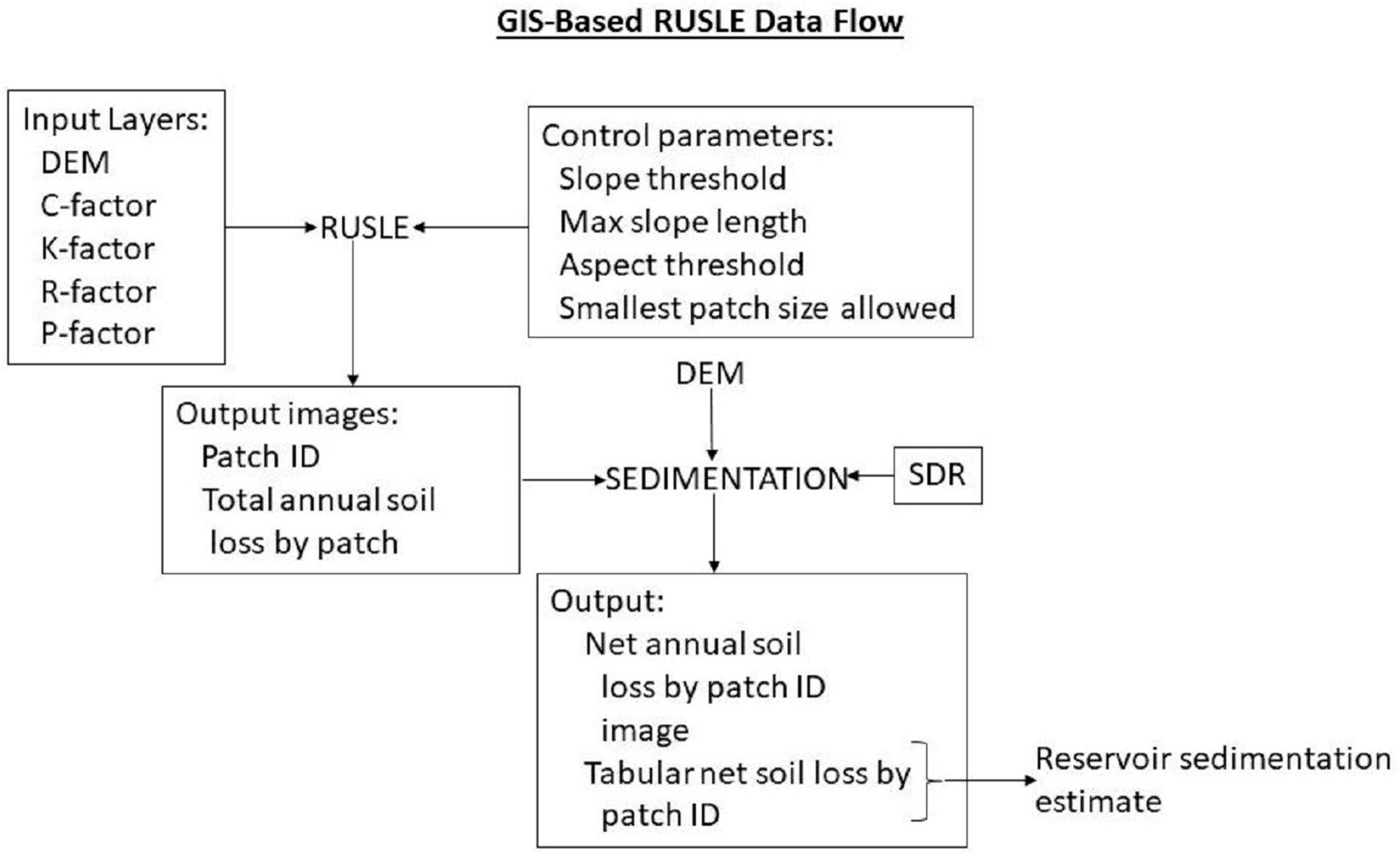
2.2. GIS-Based RUSLE/SEDIMENTATION

2.2.1. RUSLE Model Description

The RUSLE is written as follows:
A = R x   K x   L S x   C x   P
where A is the calculated soil loss per unit area in units for K (metric ton × ha × hr)/(ha × MJ × mm). The R-factor accounts for the effects of raindrop impact and the amount and rate of runoff likely to be associated with rain [12]. The K and LS factors are developed with reference to a soil loss rate determined from a unit plot 22.13 m in length, continuously in clean-tilled fallow conditions, and having a 9% slope [12]. The C-factor is a ratio of soil loss from an area with a specified cover and management to that from an identical area under tilled continuous fallow conditions [12], and the P-factor is the ratio of soil loss with a support (conservation) practice like terracing to that with straight-row farming up and down the slope [12].

2.2.2. GIS-Based RUSLE Module

We used the RUSLE and SEDIMENTATION modules within the TerrSet GIS software to estimate reservoir sedimentation. Figure 3 is a schematic of the TerrSet GIS-based implementation of RUSLE. The GIS-based RUSLE requires spatially distributed data for inputs to Equation [1], and a DEM. A 2 m horizontal resolution DEM was derived for each watershed from airborne LiDaR image of the study area acquired with the USDA-NRCS. The regional image was downloaded from the USDA-NRCS Geospatial Data Gateway [36] from which each watershed was delineated and clipped. The RUSLE module uses the DEM to calculate the spatially distributed LS factors. The K-factor images for the watersheds were downloaded from the USDA Web Soil Survey website [35], clipped and resampled to match their respective DEM image characteristics. The R-factor image for each watershed was created in TerrSet by first developing a “blank” image having the same file attributes (rows, columns, upper left and lower right image coordinates, map projection, etc.) as the watershed’s DEM. Initial pixels values for the R-factor image were set equal to 0. Using the OVERLAY module in the mathematical operations tool, the 1981 C-factor image was “added” to the newly created R-factor image, whose pixels values outside the watershed boundary remained 0. Pixel values within the watershed boundary were reclassified to a value of 225, which is the value for our study area based on the isoerodent map in Renard et al. [12]. The P-factor image for each watershed was created in the same way, except that the pixel values within the watershed boundary were set to a value of 1, as this is the recommended value when the support practice(s) used is/are unknown.
Within the GIS-based RUSLE, the software partitions the landscape into homogeneous patches based on user-supplied values for slope and aspect threshold. The maximum slope length parameter represents the distance that water can flow, in sheet form, before becoming concentrated, whereas the smallest-patch-size-allowed parameter allows patches below the specified value to be merged into larger patches. In our implementation of the model, we specified a slope threshold of 3%, an aspect threshold of 45°, a maximum slope length of 121.92 m, and the smallest patch size allowed of 40,468.6 m2.
The SEDIMENTATION module uses the patch ID number and patch total soil loss images derived using RUSLE together with the watershed DEM and a sediment delivery ratio (SDR) to simulate and quantify net soil movement between patches. The SDR is applied at the patch level and the amount of soil loss between the higher and lower patch is proportional to the length of the common boundary between them. Patch level values are then summed to produce a net soil loss or deposition for the study unit. This value is multiplied by the reservoir study impoundment period to produce an estimate of reservoir sedimentation. Supplemental Figures S1–S12 show the slope, K-factor, RUSLE total soil loss by patch, and net soil loss from the SEDIMENTATION module of each watershed as used in the GIS-based analysis for 1981.
Figure 3. Schematic of the TerrSet GIS-based implementation of RUSLE and SEDIMENTATION for estimating reservoir sediment accumulation.
Land 12 01913 g003

2.2.3. GIS-Based RUSLE Inputs

For this study, we selected five dates (1981, 1985, 1989, 1994, and 1997) of land cover data previously developed for the study area [37] to estimate the long-term reservoir sediment accumulation. These dates were selected based primarily on the availability of land cover images for each of the study watersheds. Additionally, weather records for the LWREW indicated that rainfall varied from 90 to 120% of normal over the 1981–1997 period, which is representative of the area. Supplemental Table S5 provides a summary of the satellite sensors, the horizontal spatial resolution of the images, and the classification methods used to generate the land cover data sets. Additional details regarding the development of the land cover data sets are provided by Starks et al. [37]. The findings in [37] indicated that the LWREW is largely composed of grasslands (~65%) with ~16 and 13% of crops and tree/shrub, respectively. However, annual variations in these cover categories were observed in the study. The original land cover designations for these images were reclassified into either crop, grass, or tree/shrub categories. The dominant crop in this region is conventionally tilled winter wheat that is generally used as a forage for grazing cattle. We used a C-factor of 0.37 to represent this condition as suggested by the USDA-NRCS for this region of Oklahoma [38]. The C-factors for the grass and tree/shrub conditions were derived from the tabular data presented in Wischmeier and Smith [13]. The grasslands in the study area are highly variable in terms of vegetation type (native grasses vs. improved pastures), density of plants, and grazing pressure (lightly to heavily grazed). For grass lands, an average C-factor of 0.16 was used to represent the range of vegetative canopy cover types (grass, grass-like, and short brush), having at least 20% of the cover in contact with the soil surface. For the tree/shrub conditions, an average C-factor of 0.28 was used, which represented areas having appreciable brush, bushes, and trees with an average drop fall height of ~2 m, and with about 75% of the ground surface covered by the canopy. As noted above, the RUSLE support practice (P-) factor was set to 1, and the rainfall/runoff (R-factor) was set to 225. The P- and R-factors remained fixed over each year of analysis and were identical for each watershed. The slope length (L) and steepness (S) (combined into the LS) factors also remained unchanged for a given watershed over time. The LS values are calculated within the GIS model and are not provided herein.

2.2.4. SDR Models

The SDR is the ratio of sediment yield (SY) to total soil erosion (SE), where SY is the portion of SE that reaches the stream and transported via waterways to the reservoir. Measured values of SY and SE are not generally available for most small watersheds but can be estimated from similar watersheds where measured values are available. For this study, the sediment volumes, given in Table 2, are the SY measurements (over the impoundment period of interest), but no direct measurements of SE are available. One could use the RUSLE estimates of SE together with the measured SY values to arrive at SDR. However, we could not use this approach since we would be using RUSLE influenced SDR to evaluate RUSLE itself. Thus, an independent method of estimating SDR was needed.
The SDR can be estimated from models that relate to watershed characteristics such as WA, WVL, and watershed relief, or one could use SDRs generated from similar (in size, topographic characteristics, land cover, etc.) watersheds. Garbrecht [39] used the equation of Maner [40] to calculate the SDR for four watersheds within the nearby Fort Cobb Reservoir watershed and obtained values ranging from 0.0728 to 0.1145 (mean value of 0.1). Although these watersheds are in the same region as the ones used in this study, their areas are one to two orders of magnitude larger; thus, the mean SDR value for these four watersheds may not be representative of our study watersheds. The Maner [40] equation is as follows:
L o g S D R % = 2.94259 0.82362 × L o g W v l W r l f
Equation (2) was applied to the study watersheds and the results reported in Table 2. We also computed the SDR from the models of USDA [41] (Equation (3)), Boyce [42] (Equation (4)), and Vanoni [43] (Equation (5)), all of which are related to WA.
S D R = 0.5656 × W A 0.11
S D R = 0.3750 × W A 0.2382
S D R = 0.4724 × W A 0.125
where WA is in km2. The results of these equations are also provided in Table 2.
Table 2. Sediment delivery ratio (SDR) values for each watershed calculated using Equations (2)–(5).
SDR Models
Watershed IDEquation (2)Equation (3)Equation (4)Equation (5)
110.2540.4740.2570.387
140.2600.4350.2130.351
200.2480.4580.2380.372
210.3720.5040.2930.415
220.3640.5030.2910.414
230.2680.5110.3020.421
240.2290.4560.2360.37
260.1030.4110.1880.329
310.1790.4080.1860.327
390.2550.4610.2420.375
410.3210.5240.3180.433
420.3950.5270.3220.436
As observed from Table 2, the four models produced a wide range of values for a given watershed. The GIS-based RUSLE model (for all watersheds and dates) was run for each SDR model, and the resulting sedimentation estimates (NDRes; see Equation (6) below) were compared. Example images of RUSLE total annual soil loss by patch and SEDIMENTATION net annual soil loss by patch are provided in Supplemental Figures S1–S12. Although Equation (2) resulted in the smallest mean NDRes value (Table 3), it also had the largest standard deviation. Based on the findings provided in Table 3, SDR values computed via Equation (3) were chosen, as they produced the smallest standard deviation between estimated and measured reservoir sedimentation (Table 3).

2.3. Normalized GIS-Based RUSLE Reservoir Sedimentation Estimates

Average annual soil loss was determined for each watershed for each of the five years. The annual soil losses were multiplied by the respective reservoir’s impoundment period (Table 2) and sediment bulk density [1] to estimate reservoir sedimentation for comparison against measured values (Table 2). The resulting estimated sedimentation values were normalized (NDRes) with reference to the measured sedimentation data acquired from the bathymetric survey for the respective reservoir according to the following:
N D R e s = E s t i m a t e d   S e d i m e n t a t i o n M e a s u r e d   S e d i m e n t a t i o n M e a s u r e d   S e d i m e n t a t i o n × 100 ,
where positive values of NDRes indicate percentage overestimation relative to the measured values and negative values indicate percen underestimatation.

2.4. Stream Bank Sediment Contributions

2.4.1. First-Order Adjustment

Ref. [27] showed, for a stream near our study area, that ~54% of the suspended sediment in stream flow was due to stream bank sources. Assuming that this finding is applicable to other streams near the study region, the measured reservoir sediment values were decreased by 54% before comparing them against GIS-based RULSE estimates.

2.4.2. Statistical Linkages between NDRes and Watershed, Stream, Stream Corridor, and Within-Channel Variables

In contrast to the regional adjustment approach in Section 2.4.1, we developed watershed, stream, stream corridor, and within-channel variables (described below) as possible indicators of sediment contributions from gullies, stream banks, or stream channels.

2.5. Statistical Analysis

The various data types (RUSLE inputs, watershed, stream, stream corridor, within-channel, and NDRes) were analyzed in JMP 17 Pro (SAS Institute, Cary, NC, USA) to produce basic descriptive statistics and to evaluate differences between estimated and measured sedimentation as a function of year of land cover (C-factor) acquisition, subdominant land cover, and other variables, and for identifying variables that may be predictive of the discrepancy between measured and modeled reservoir sedimentation. All non-normal data were transformed before analysis.

3. Results and Discussion

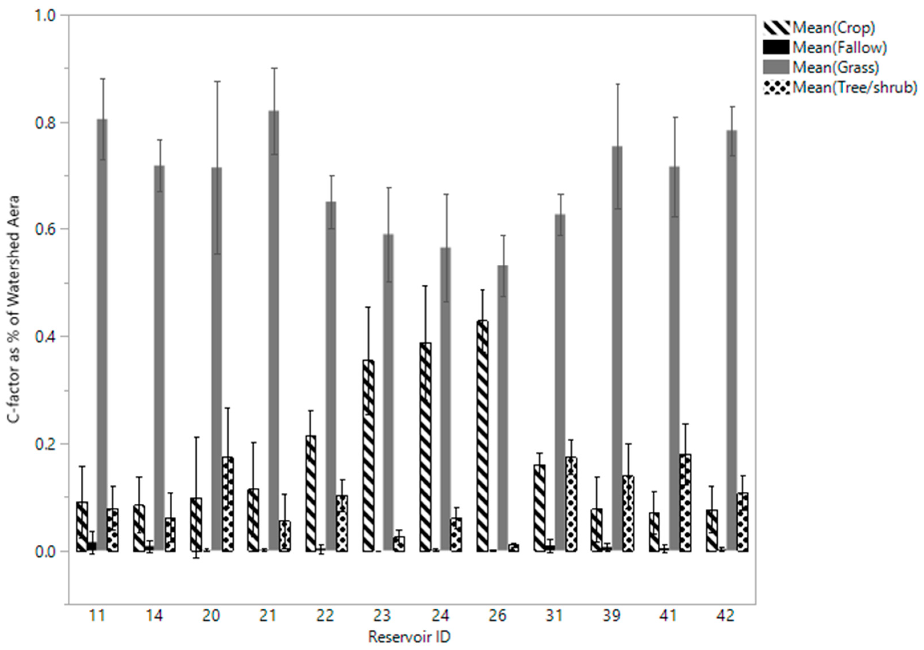
3.1. Variability in RUSLE C- and K-Factors

3.1.1. C-Factors (Land Cover)

Satellite data from five dates were used to quantify land area within a given watershed in either crops, grass, tree/shrub, or fallow. It was expected that small changes in land cover area between years would occur, but the actual magnitude of these changes and their impacts on the estimates of reservoir sediment accumulation were unknown. An example of temporal variability of land cover within Watershed 24 is provided in Table 4 where it is observed that watershed area associated with trees/shrubs increased from ~6% in 1981 to ~9% in 1989 but occupied ~4% of the watershed area in 1994 and 1997. The largest temporal changes occurred in the cropland and grassland subdominant land cover groups. This is not uncommon in areas where some agricultural producers may shift from grazing livestock to planting alfalfa, cereal grains, or other crops, or conversely, where some cropland may be converted back to grassland, possibly to take advantage of changing cattle markets or to participate in conservation programs. An example of such a large temporal change in the crop and grass groups is observed in 1989, whereas in the years prior to this, cropland accounted for 41 to 47% of the watershed area. However, that percentage was greatly reduced in 1989 when cropland accounted for ~18% of the watershed area. Fallow ground was observed in 1981 and 1985, but the percentage of watershed areas was less than 1%. Large temporal changes between cropland, grassland, and tree/shrub lands are observed for other watersheds in this study (Figure 4 and Supplemental Table S6). Fallow ground was < 6.3% in all watersheds but averaged ~0.7% across all watersheds and satellite land cover dates (Supplemental Table S6).
The C-factor values are directly linked to the cover type; thus, Table 4 (and Supplemental Table S6) can also be interpreted as the total watershed area associated with a given C-factor. The largest C-factor (1) is associated with fallow ground, which occupies a small area in Watershed 24 (Table 4). However, the cropped area (C-factor = 0.37) ranged from 18 to 47%. Thus, it could be expected that soil erosion was highest in 1989, depending upon timing, amount, and rates of rainfall during that year, all other things being equal. The C-factor associated with the tree/shrub category (C-factor = 0.28) occupied from ~4 to ~9% of the watershed area, depending on year, whereas the C-factor associated with the grass category (C-factor = 0.16) varied from ~48% to ~75% of the watershed’s total area. Watershed C-factor images for each of the five dates are provided in Supplemental Figures S13–S24.
Table 4. Decimal percentage of total watershed area, by year, under either crop, grass, tree/shrub, or fallow ground, for Watershed 24.
Image Year
Cover Type19811985198919941997
Crop0.4710.4140.1790.3940.445
Fallow--0.0020.005----
Grass0.4880.5440.7520.5940.537
Tree/Shrub0.0640.0640.0880.0350.042
Figure 4. Mean of total watershed area under a given C-factor (or land cover type) for the watershed indicated. One standard deviation is indicated for each bar.
Land 12 01913 g004

3.1.2. K-Factors

The soil erodibility (K-) factors are different in value, distribution, and number for each watershed but remained static for a given watershed regardless of the year of analysis (Table 5, Supplemental Figures S1–S12). Zero (0) values indicate no soil erodibility and correspond to percentage of water surface in each watershed. Such values could also indicate impervious surfaces, but surfaces of this type were not apparent in the K-factor data. It is readily observed from Table 5 that Watersheds 22, 23, 24, 26, and 31 have ≥ 55% of their areas in soils with K-factors ≥ 0.37 (moderate to highly erosive soils). Watershed 11 has ~31% of its area in these moderate to highly erosive soils, whereas the remaining watersheds have ≤ 14%. Watershed area-weighted K-factors ranged from 0.16 (Watershed 14) to ≥ 0.30 for Watersheds 22, 23, 24, 26, and 31.

3.2. Initial Reservoir Sedimentation Analysis

All NDRes were pooled over satellite land cover date within and across the subdominant watershed landcover categories and summary statistics calculated (Table 6). From this analysis, it was observed that for all watersheds combined, the GIS-based RUSLE model underestimated accumulated reservoir sediment by ~62%, on average. However, there was a considerable difference between maximum and minimum NDRes. At the subdominant land cover category level, the Crop watershed group exhibited the largest variability in NDRes, ranging from an overestimation of ~333% to an underestimation of ~98% (CV = 339%). The Grass and Tree/Shrub groups exhibited smaller ranges (CVs = 64.7 and 13.6%, respectively), with average NDRes values of ~−72 and −83%, respectively.
Further analysis indicated that the annual estimates of reservoir sedimentation were not normally distributed. These data were subsequently normalized (NDResT) using a Johnson SU transformation [44]. After the transformations, the data were subjected to ANOVA and Student’s t-test to further investigate any statistical differences in the subsequent estimates of NDRes and NDResT as a function of land cover date used to determine the C-factors, and to investigate differences in NDRes within and across watershed subdominant land cover group, and across individual watersheds.

3.3. Effects of Land Cover (C-factor) Date on Sedimentation Estimates

3.3.1. Date Effects Pooled over All Watersheds

ANOVA of the NDResT data indicated that the various satellite dates did not produce statistically significantly different estimates of sedimentation (p = 0.6352). Student’s t-test further corroborated the ANOVA results (Table 7). In practical terms, however, if the 1985 C-factors were used to estimate the long-term reservoir sedimentation, this would produce an average underestimation of reservoir sedimentation of ~42%, while the 1994 land cover data would have produced an average underestimation of ~79%

3.3.2. Date Effects within Watershed Subdominant Land Cover Group

ANOVA of the NDResT data indicated no statistically significant effects of year of land cover date within either the Crop or Grass subdominant land cover categories (p = 0.4482 and 0.68901, respectively). Student’s t-test further corroborated the ANOVA results (Table 7). However, the ANOVA for the Tree/Shrub group of watersheds did indicate that at least one of the land cover dates produced estimates of NDResT that were statistically different from estimates generated from one or more of the other dates. According to the t-test, the C-factors generated from the 1985 land cover data were statistically distinct from that generated using the 1989 land cover data.
In practical terms, estimated reservoir sedimentation within the reservoirs assigned to the Crop category of watersheds ranged from an overestimation of ~27% in 1985 to an underestimation of ~76% in 1981. For reservoirs within the Grass group, all years were associated with underestimates of measured reservoir sedimentation, ranging from −81% (1985) to −58% (1997). Similarly, all model simulations of reservoir sedimentation in the Tree/Shrub category of watersheds underestimated measured values, ranging from −91% (1989) to −71% (1985).
Table 7. Least square means * of NDResT as a function of land cover/C-factor date within the subdominant landcover groups.
DateAllCropGrassTree/Shrub
19810.4380.5100.4810.323 ab
19850.5450.6180.4220.593 a
19890.4990.8430.4620.193 b
19940.4540.5650.4010.395 ab
19970.5950.7380.6670.369 ab
* NDResT means not connected by the same letter are significantly different (α = 0.05).

3.4. Comparison of Averaged Estimated and Measured Reservoir Sedimentation

Although not statistically significant, given the large practical differences between estimated and measured reservoir sedimentation, the analyses reported below are based on the GIS-based RUSLE simulations for all years and watersheds.

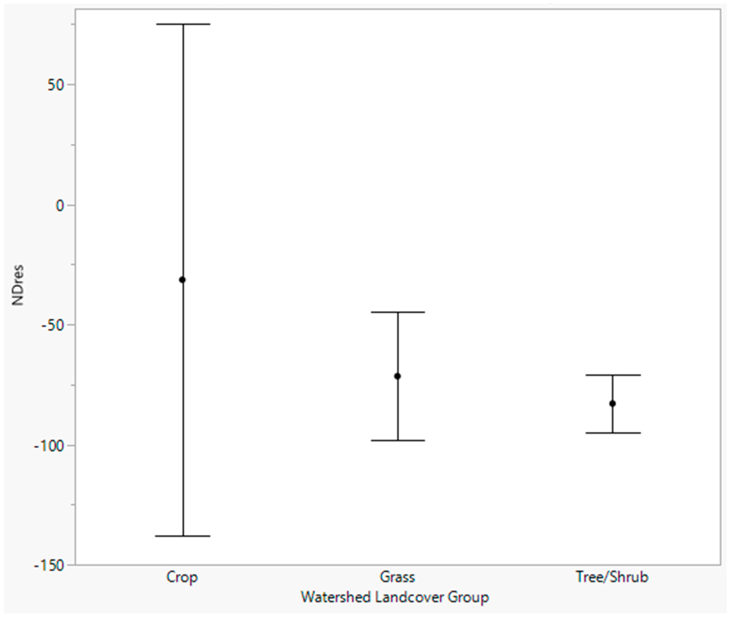
3.4.1. Between Subdominant Land Cover Groups

The ANOVA of NDResT, pooled over date within watershed subdominant land cover groups (Table 8), indicated that at least one watershed land cover group represented a different population (p = 0.004). Figure 3 indicates that the corresponding NDRes values are more variable over time for Crop watersheds than those for the Grass and Tree/Shrub watersheds. Although the NDResT for the Grass and Tree/Shrub groups are statistically similar, the Tree/Shrub group’s standard deviation is about half of that of the Grass watershed group. On average, the estimated reservoir sedimentation from the Crop, Grass, and Tree/Shrub watersheds underestimated measured values by 31, 71, and 83%, respectively (Figure 5).
Table 8. Results of Student’s t-test on NDResT, pooled over date within watershed subdominant land cover group.
Watershed Land Cover* NDResT Least Square Mean
Crop0.655 a
Grass0.489 b
Tree/shrub0.374 b
* Means not connected by the same letter are significantly different (α = 0.05).
Figure 5. Plot of mean NDRes (solid circle) by watershed subdominant land cover group. Error bars indicating one standard deviation above and below the mean value are also shown.
Land 12 01913 g005

3.4.2. Between Reservoirs within Subdominant Land Cover Group

ANOVA of average watershed NDResT within the Crop and Grass subdominant land cover groups indicated that at least one watershed within each group produced a NDResT that represented a different population when compared to other watersheds within the group (p = 0.03 and 0.01, respectively). The ANOVA for the Tree/Shrub group indicated that the watershed NDResT estimates were all drawn from the same population (p = 0.4442). Student’s t-test (Table 9) indicated that, in the Crop watershed group, the NDResT for Watershed 31 was statistically different from the remaining watersheds within the group. The Grass group watersheds exhibited more statistical differences among themselves than those observed for the other two subdominant land cover watershed groups. In the Grass group, it was observed that Watershed 11 generated NDResT values that were statistically different from those for Watersheds 21 and 14, whereas Watershed 14 values were statistically dissimilar to Watersheds 11 and 22.
The actual NDRes values for the Crop group of watersheds indicate that reservoir sedimentation estimates ranged from an underestimation of ~83% (Watershed 31) to an overestimation of ~24% (Watershed 23). All model simulations underestimated reservoir sedimentation for all watersheds within the Grass group and ranged from ~−50% (Watershed 11) to ~−89% (Watershed 14). Model simulations for the Tree/Shrub watersheds underestimated measured values for all watersheds and ranged from ~−77% (Watershed 41) to ~−89% (Watershed 20).

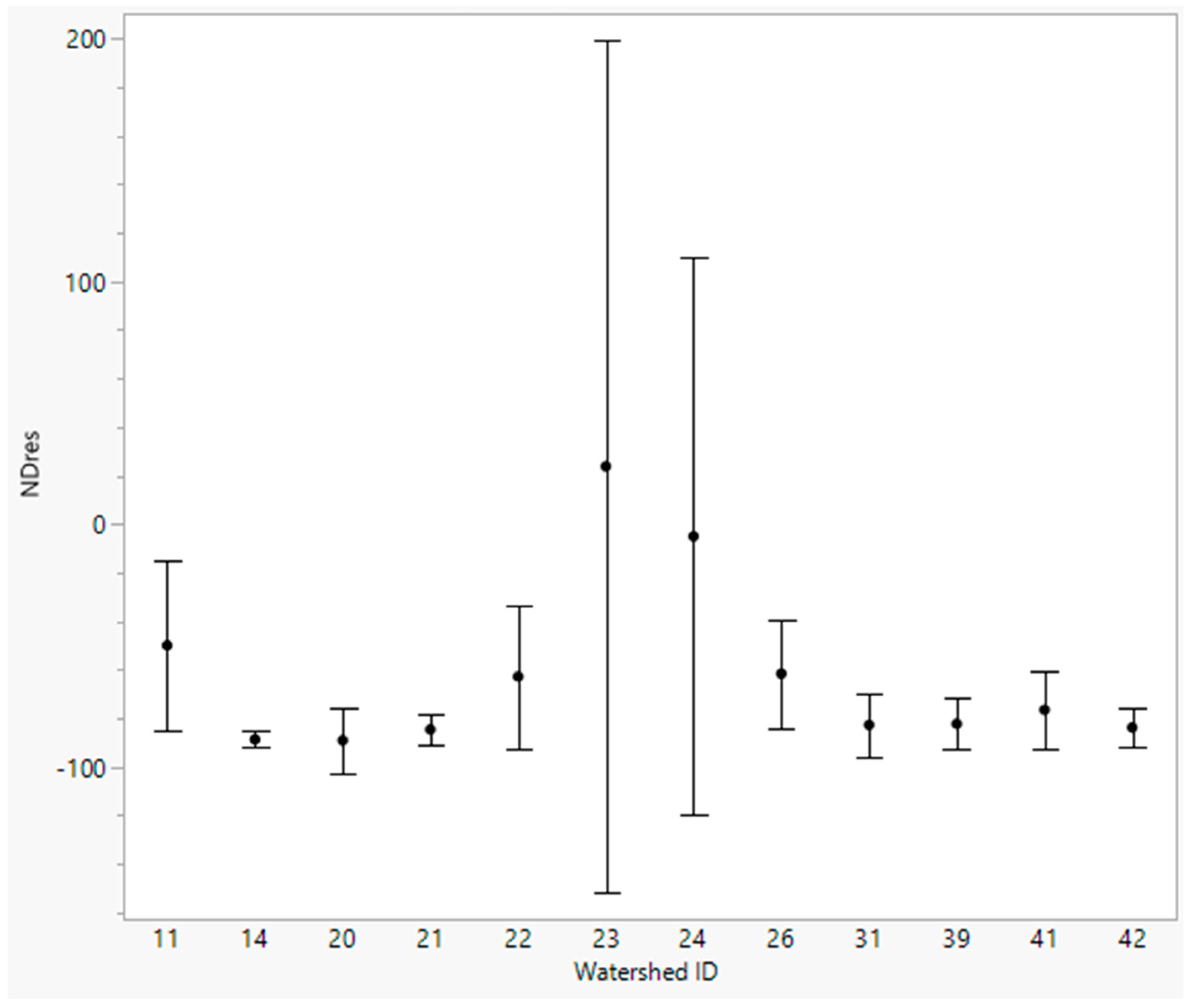
3.4.3. Across All Watersheds

The ANOVA indicated that NDResT of at least one watershed represented a different population (p = 0.0004). Results of the Student’s t-test are provided in Table 10, where values shown in the table are the same as those provided in Table 9 but are ranked with respect to each other.
Watershed 23 was the only 1 of the 12 watersheds that produced a positive mean NDRes value (Figure 6). However, this watershed exhibited the most variable results (Figure 6), followed closely by Watershed 24. The high variability in these two watersheds (both members of the Crop subdominant land cover group) is due to a single comparatively high NDRes value. For Watershed 23, a NDRes of over 300% occurred in 1985, whereas a value of nearly 200% for Watershed 24 occurred in 1989. Removal of these two data points brings the mean NDRes values to −53.4% for Watershed 23, and to −56.0% for Watershed 24 (Table 11). Although the prior Crop watershed mean NDRes was negative (Table 6), it became more negative (−64.4%; calculated from the values provided in Table 11) with the removal of these two data points, bringing the subdominant land cover group of reservoir’s NDRes average in closer agreement with that of the Grass and Tree/Shrub group.
If the NDRes values generated from the 1985 and 1989 dates for Watersheds 23 and 24, respectively, are outliers, then reanalysis of the data set indicates that the overall average underestimation of reservoir sedimentation is 72.6% ± 14.8%, and that the watershed mean NDRes values range from −50% (Watershed 11) to −89.2% (Watershed 14) (Table 11). From inspection of the NDResT values and their statistical similarity designations, two broad groups emerge and are as follows: Group 1 (all connected by the letter “a”) consisting of Watersheds 11, 22, 23, 24, and 26, and Group 2 (all connected by the letter “e”) consisting of Watersheds 14, 20, 21, 31, 39, 41, and 42 (Table 12). The NDRes mean for Group 1 is −56.8 ± 5.4%, and the Group 2 mean is −84.0 ± 4.3%. The Group NDRes means are statistically different at the α = 0.05 level.
Table 11. Results of Student’s t-test performed on the NDResT pooled over year excluding two “outlier” land cover/C-factor dates and their associated mean NDRes and the NDRes adjusted for first-order contribution of steam bank/channel sedimentation (NDRes_adj) for each watershed.
Watershed/Reservoir IDWatershed Land Cover Group* NDResTNDRes
Mean
(%)
NDRes_adj
Mean
(%)
24Crop0.763 a−56.0−4.3 abc
11Grass0.726 b−50.08.7 a
26Crop0.681 ab−61.6−16.6 abcd
23Crop0.679 abc−53.41.4 ab
22Grass0.589 abcd−62.8−19.2 abcd
41Tree/shrub0.476 abcde−76.5−49.0 bcde
39Tree/shrub0.417 bcde−82.3−61.5 cde
31Crop0.387 cde−82.7−62.5 cde
42Tree/shrub0.383 cde−83.8−64.8 de
21Grass0.370 de−84.6−66.6 de
14Grass0.269 e−88.9−75.9 e
20Tree/shrub0.222 e−89.1−76.3 e
* NDResT least square means followed by different letters are significantly different (α = 0.05) (the data used to derive the NDRes values provided in Table 11 are used in the analyses reported in subsequent sections).

3.5. Stream Bank Contributions—First-Order Adjustment

The results of this adjustment (NDRes_adj) are provided in the right-most column of Table 11, where it is observed that the discrepancy between the estimated and measured values of reservoir sedimentation for Reservoirs 11, 22, 23, 24, and 26 was under 20% (absolute), averaging −6.0 ± 11.8%. However, the NDRes_adj for the remaining seven watersheds ranged from −49.0% (Reservoir 41) to −76.3% (Reservoir 20). It was observed that NDRes_adj for Reservoir 41 was more statistically like Group 2 (ending statistical similarity designator = e) than Group 1 (ending statistical similarity designator = d). The mean NDRes for Group 2 is −65.1 ± 9.3%. The difference between the two groups after adjusting for stream bank contributions suggested that a regionally based adjustment for gully or stream bank sediment contributions would not be sufficient to account for RUSLE’s weakness in this area. Thus, further analysis was needed to identify watershed, stream, stream corridor, or within-channel characteristics that may be used as proxies to account for sediment contributions derived from gullies, stream channels, or stream banks.

3.6. Watershed, Stream, Stream Corridor, and Within-Channel Variables

3.6.1. Watershed and Stream Variables

Generally, the watersheds are of moderate-to-low relief with an average basin relief of ~51 m and range from a high of ~78 m (Watershed 31) to a low of 38 m (Watershed 21) (Supplemental Table S7). The %Wslope≥21 varied from a low of 0.3% (Watersheds 39 and 41) to a high of 9.7% (Watershed 22), averaging ~2.3 ± 2.7% across all watersheds. The Wvl averaged 4135 m across all watersheds but is quite variable ranging from 1761 m (Watershed 21) to 11,002 m (Watershed 26). Similarly, Sthal varied from 13,196 m (Watershed 31) to 1844 m (Watershed 21), averaging 4939 ± 3406 m. The Sslope were gentle for all watersheds, averaging 0.013 ± 0.005 m m−1, while Ssn values indicated that five of the streams are essentially straight (Ssn < 1.05), while the remaining seven streams have low sinuosity (1.06 > Ssn ≤ 3.0).
Watershed topographic and general stream characteristics are presented in Table 12 where it is observed that the two groups are statistically similar in terms of WA, Wrlf, %Wslope ≥ 21, Sthal, Sslope, and Ssn. However, the two groups statistically differ in percent of watershed area in %WLK, %WMK, and %WHK. Watersheds in Group 2 have, on average, ~74% of their areas in %WLK with about 72% of these soils having a value ≤ 0.2 (Table 5). Watersheds in Group 1 have ~66% of their areas in %WMK, with ~47% of these soils having a value ≥ 0.37 (Table 5). Additionally, Group 1 watersheds have another 13% of their areas in high K-factors soils, indicating that Group 1 watersheds have more erosive soils than those observed in the Group 2 watersheds.
Table 12. Comparison of Group 1 and 2 least square means of watershed area (WA), watershed basin relief (Wrlf), percent of watershed area with slopes ≥ 21° (%Wslope>21), percentage of watershed area in low, moderate, or high K-factor soils (%WLK, %WMK, and %WHK), stream thalweg length (Sthal), stream slope (Sslope), and stream sinuosity (Ssn).
Watershed Variables *Stream Variables
Broad Group IDWA (km2)Wrlf
(m)
%Wslope≥21Wvl%WLK%WMK%WHKWKSthal
(m)
Sslope
(m m−1)
Ssn
17.151.01.7510119 b66 a13 a0.33 a60780.0111.21
27.151.51.0375374 a19 b3 b0.21 b41240.0151.09
* Means not connected by the same letter are significantly different (α = 0.05).

3.6.2. Stream Corridor Variables

The%Corslope≥21 ranged over two orders of magnitude from 0.6% (Watershed 39) to 9.7% (Watershed 42) and to 36.8% (Watershed 21) (Supplemental Table S8). The%Corslope ≥21 for Watersheds 21, 23, and 31 averaged 28.5 ± 12.7%, and it averaged 5.5 ± 3.3% over the remaining watersheds. The Corslope≥21:WVL varied from 1.8 m2m−1 (Watershed 41) to 36.8 m2m−1 (Watershed 22), averaging 9.5 m2m−1 over the 12 study sites (Supplemental Table S8). The %CorLK, %CorMK, and %CorHK variables averaged 47.6, 48.4, and 4.0%, respectively, over the study sites. However, considerable variability was observed between sites for all three K-factor categories. For example, the corridors in Watersheds 14 and 41 had 100% of their areas in low K-factor soils, whereas Watersheds 24 and 26 had 5.8 and 0.3%, respectively (Supplemental Table S8). Moderate K-factor soils occupied ≥ 70% of corridor areas in Watersheds 21, 22, 23, 24, 26, and 31. High K-factor soils were not present in the corridors of Watersheds 11, 14, 21, 39, and 41 and accounted for ≤5% in Watersheds 22, 23, 31, and 42. Watershed 26 had the largest corridor area in high K-factor soils at ~26%.
Low K-factor soils in the 100 m stream corridor (%CorLK) are statistically and significantly more prominent in the Group 2 watersheds (~67%) than in Group 1 watersheds (~20%) (Table 13). Conversely, ~80% of the Group 1 corridor is in moderate-to-high K-factor soils. The %Corslope ≥21 is statistically similar between groups, but in practical terms, the Group 2 watersheds have twice their corridor areas occupied by slopes ≥ 21° as compared to the Group 1 watersheds. Interestingly, however, Corslope>21:Wvl is statistically and practically higher in Group 1 corridors containing about three times more area with slopes > 21° per m of Wvl. This variable may be an indicator of bank instabilities and/or development of gullies along the main channel of the stream and its tributaries, and therefore, they are potential sources of sediments for which the GIS-based RUSLE cannot account.

3.6.3. Within-Channel Variables

The BFD varied from 0.22 m (Watershed 42) to 1.29 m (Watershed 31), averaging 0.6 m over all 12 study sites (Supplemental Table S9). On average, the BFW was about 40 times the BFD but varied from ~13 (Watershed 23) to ~99 (Watershed 11) times larger than the BFD (see BFW:BFD in Supplemental Table S9). The BAs were found to be low for all streams as they were generally ≤ 20° (Supplemental Table S9). Average BH was 2.4 m, which is categorized as very high (Supplemental Tables S3 and S7), but varied from 0.65 (Watershed 11) to 4.14 m (Watershed 22). Of the 12 study sites, BH was ≥2.1 m (very high, Supplemental Table S3) for all but Watersheds 14, 39, 41, and 42. The BHR averaged 4.5, which is classified as highly unstable (Supplemental Tables S2 and S9). The BHR value for all sites indicated that all stream banks were unstable (Supplemental Tables S2 and S9). The ER for all streams indicated that they were slightly to moderately entrenched as ER was generally ≥ 1.4 (Supplemental Tables S4 and S9), with an overall average of 3.5. On average, CD was 2.9 m, CW was ~38 m, and CA was ~80 m2. However, CD, CW, and CA varied considerably (Supplemental Table S9).
The two groups are statistically similar with regard to CD, CW, CW:CD, and CA (Table 14). However, the stream channels are, on average, about 1.2 m deeper in Group 1 than those in Group 2. This difference in CD accounts for the rather large disparity, although not statistically significant, between the CW:CD values, i.e., for Group 1, the mean stream CW is ~18 times the CD, whereas the CW for Group 2 is ~36 times the CD. The CA of the Group 1 streams is ~1.5 times larger than that of Group 2. Except for BHR, the stream bank variables are not statistically different between the two groups. Although not statistically different, the ER values indicate that Group 1 streams are moderately entrenched, whereas Group 2 streams are slightly entrenched (Table 15 and Supplemental Table S4). For Group 1, the ER suggests that the streams are somewhat disconnected from their floodplains; thus, sediments derived from various sources are likely to stay within the streams and be more efficiently moved to the receiving reservoir. Conversely, the streams in Group 2 are more connected to their floodplains; thus, sediments derived from various sources could be re-deposited within the floodplain increasing their residence time within the watershed before ultimately being deposited into the receiving reservoir. The BA values are classified as low (Supplemental Table S3) for both groups and are not statistically different. The BH values are also not statistically different between the two groups; however, BH for the Group 1 streams is classified as “extreme”, while it is classified as “high” for Group 2 steams (Supplemental Table S3). The Group BHR values are statistically different, and both values indicate highly unstable banks (Supplemental Table S1)—but more so for streams in Group 1. The BA, BH, and BHR data indicate that the banks and channels in Group 1 likely contribute more sediments to their streams than do the stream banks in Group 2. Group means of FWA_%WA were not statistically different, but values ranged from a low value of 1.56 (WS 14) to 5.71 (WS 23) (Supplemental Table S9).
Except for Watershed 26, ICSa ≥ 41% (Supplemental Table S10), averaging 51.8 ± 13.8% over all sites. The ICSi varied from 18% (Watershed 41) to 56% (Watershed 26). Low K-factor soils dominate in the streambed and stream banks of Watersheds 11, 14, 20, 39, 41, and 42, but moderate K-factor soils make up > 55% of the area in the remaining study sites. In fact, moderate K-factor soils make up > 91% of the streambed and stream bank soils in Watersheds 22, 24, and 26. High K-factor soils make up < 0.5% of the soils in Watersheds 20, 22, and 31 with the remaining sites having no high K-factor soils present. The plasticity index (ICPI) varied from a low of 4.6 (Watershed 41) to a high of 17.3 (Watershed 26) (Supplemental Table S10).
In terms of the within-channel soils variables, the Group 1 soils have a larger silt (ICSi) and smaller sand fractions (ICSa) than soils in Group 2 (Table 15). Correspondingly, the within-channel soils for Group 1 have K-factors that are predominantly (~78%) moderate in value, whereas the Group 2 stream channel and stream bank soils are predominantly (~74%) low in value. High K-factor soils accounted for < 1% of the soils in both groups, with no statistical differences between the groups. On average, the stream channel and stream bank soils in Group 1 soils have statistically larger K-factors (0.33) than those in Group 2 (0.23) and are, therefore, more erosive. The %ICPI of the stream channel and stream bank soils is not statistically different between groups, although the value for Group 1 is ~1.4 times larger than that of Group 2.
Table 15. Least square means of within-channel (IC)-weighted soil K-factor (ICK), sand (ICSa), and silt (ICSi) fractions, percentages of low, moderate, and high K-factor soils (%ICLK,%ICMK, and %ICHK), and weighted average plasticity index (ICPI) for each group’s stream channels and stream banks.
Group IDICK *ICSaICSi%ICLK%ICMK%ICHKICPI
10.33 a40.8 b37.2 a21.6 b78.2 a0.1410.9
20.23 b59.6 a23.1 b73.9 a25.1 b0.097.6
* Means followed by different letters are significantly different (α = 0.05).

3.7. Sediment Delivery Ratios (SDRs)

Setting the SDR to one forces the SEDIMENTATION module to route all RUSLE-simulated soil erosion through the watershed to the receiving reservoir, thereby providing a maximum sedimentation estimate. Comparison of GIS-based RUSLE simulations where SDR = 1 (all years, all watersheds) revealed that average watershed sedimentation overestimated measured values from ~1200% (Watershed 14) to ~22,000% (Watershed 23). Because the SEDIMENTATION module applies the SDR to each patch and because the amount of soil moving from one patch to the next is proportional to length of the common boundary between the two patches, sediment movement and delivery to the reservoir are reduced beyond a simple multiplication of the SDR and the RUSLE estimate of overland soil erosion. Thus, it is fortuitous that the combination of the first-order adjustment and the SDRs used in the GIS-based RUSLE simulations for the Group 1 watersheds worked as well as they did. However, this combination did not work as well for the Group 2 watersheds. The persistent and large underestimation of measured reservoir sedimentation in Group 2 watersheds after the first-order adjustment implies that the SDRs used for these watersheds are too high (i.e., too much sediment is allowed to pass through the watershed to the reservoir), or that the assumed amount of sediment generated from channels, banks, and gullies is too large. We have no information for our region than that provided by Wilson et al. [29] regarding sediments derived from channel, bank, and gully sources. Therefore, the impact of lowering the SDR to 0.1 for the Group 2 watersheds based on the study of Garbrecht [39] was investigated, while at the same time maintaining the first-order adjustment for stream channel, stream bank, and gully sediment contributions. This value for the SDR was helpful in some instances, but the underestimation remained large for some watersheds (Supplemental Table S11). Watershed 31 improved from a large underestimation to a moderate underestimation, and Watersheds 41 and 42 changed from a large underestimation of measured reservoir sedimentation to moderate overestimations (24.3 and 18.7%, respectively, Supplemental Table S11), implying that an SDR value between 0.1 and that calculated from Equation (3) could improve agreement between estimated and measured sedimentation, but without measurements of actual soil erosion, selection of the appropriate SDR would be subjective. Large underestimations were persistent for Watersheds 14, 20, 21, and 39. These findings suggest that an unrealistically small SDR would be needed to bring estimated and measured reservoir sedimentation into closer agreement.

3.8. Watershed, Stream, Stream Corridor, and Within-Channel Variables as Predictors of NDRes

We developed a series of prediction equations using stepwise regression relating the variables to NDRes but limited the number of variables to five to minimize over-fitting the equations. The best models are shown in Table 16 (alternative models are provided in Supplemental Table S12). The best one-variable model used accounted for ~44% of the variability of NDRes using LNWSK. The equation indicates that as the overall watershed soil erosivity increased, NDRes became less negative. Refs. [19,20] noted that RUSLE erosion estimates were >100% in some instances. Assuming the RUSLE overestimates soil erosion, the equation implies that the dominance of highly erosive soils in a watershed may compensate, to some degree, the RUSLE bias or “baseline” effect when trying to estimate reservoir sedimentation. However, the amount of overestimation is unknown for our watersheds. The one-variable model cannot account for well over one-half of the variation of NDRes, thereby limiting the usefulness of this model. The two-variable model accounted for ~72% (adjusted R2) of the variability in NDRES using SHASHER and FWA_%WA. As ER increases (i.e., stream entrenchment decreases), underestimation of measured reservoir sedimentation increases. Less entrenched streams are better connected to their floodplains [31] providing an increased opportunity for the redeposition of sediment (from all sources), thereby impeding and delaying sediment delivery to the receiving reservoir. This, in combination with the assumed RUSLE overprediction of soil erosion, may account for the increased discrepancy between the GIS-based RUSLE estimates of reservoir sedimentation and observed data. The FWA_%WA variable somewhat mitigates the effects of the ER variable because, as it increases, the NDRes value becomes less negative. This may be due to probable increased generation of sediments by larger FWAs (i.e., larger wetted perimeter) as compared to those that are smaller. The three-variable model included LNBFD, FWA_%WA, and ICK and accounted for ~82% of the variability in NDRes. The role of FWA_%WA is the same as that described for the two-variable model, and the role of ICK is like that described for WSK in the one-variable model; however, the relationship between ICK and NDRes is stronger than that of WSK and NDReS. As the BFD increases, the NDRes becomes increasingly negative. Larger BFDs indicate that more stream bank area is exposed to erosive processes, thereby contributing more sediment to the receiving reservoirs and for which the RUSLE model cannot account [19]. The four-variable model accounts for ~95% of the variation in NDRes and includes the previously discussed WSK and ER variables as well as the log-normal versions of Wvl and Corslope≥21:Wvl. Regarding Wvl, it is noted that as the value of this variable increases so does the degree of underestimation of measured reservoir sedimentation. This variable may be related to an increasing probability of sediment contributions from gullies, stream channels, and stream banks as the watershed valley length increases. The Corslope≥21:Wvl behaves similarly to Wvl, but is a better indicator of likely gully and stream bank sources of sediment within the 100 m corridor of the stream not accounted for by the RUSLE model. The five-variable model accounts for ~98% of the variability of NDRes and includes one variable not discussed heretofore—the WA. From the regression model, it can be noted that as WA increases, the underestimation of measured sedimentation decreases. This variable is likely related to the SDRs used in the GIS-based RUSLE/SEDIMENTATION simulations of the respective watersheds. As noted earlier, the SDR is based on WA and has been formulated on the general observation that as WA increases, sediment delivery to the receiving reservoirs decreases.

4. Conclusions

Three objectives guided this research study. Objective 1 sought to evaluate the impact of temporal variations of the RUSLE C-factor on the estimation of reservoir sedimentation. To this end, we used land cover maps to determine C-factors of five dates for 12 watersheds located in the Little Washita River Experimental Watershed. Evaluation of the GIS-based RUSLE simulations indicated that there were no statistical differences in the sedimentation estimates when all watersheds were pooled over all dates. Yet, there were large practical differences between some years. There were also no statistical differences in estimates of reservoir sedimentation within the Crop and Grass subdominant land cover groups; however, there were statistical differences between the 1985 and 1989 dates within the Tree/Shrub group. For reservoir sedimentation studies, it is advisable to run simulations for several different years to capture the impact of temporally variable C-factors to better account for variations in overland sediment contributions to reservoir sedimentation.
It has been noted that a primary weakness of RUSLE is its inability to account for sediments derived from gully, stream channel, and stream bank sources. In Objective 2 we conducted a first-order (regionally based) adjustment to compensate for these sources by reducing the measured reservoir sediment. This adjustment resulted in closer agreement between estimated and measured sedimentation for all 12 watersheds, but better agreement occurred for five watersheds where the difference between GIS-based RULSE estimated and measured sedimentation averaged −6.0 ± 11.8%. Although the agreement between estimated and measured reservoir sedimentation improved somewhat for the remaining seven watersheds, average underestimation was still large (−65.1 ± 9.3%). Thus, it is apparent that a regionally based adjustment will not likely be adequate to bring RUSLE-based estimated of reservoir sedimentation in line with measured data. It was also shown that unrealistic SDRs would be required to bring model simulations of reservoir sedimentation into agreement with measured data, under the conditions specified in this study.
Analyses of the linkage between watershed, stream, stream corridor, and within-channel variables (objective 3) showed strong relationships between selected geomorphic, pedologic, and topographic variables and the degree to which measured reservoir sedimentation was underpredicted using the GIS-based RUSLE model. The parameter values for the linear regression models developed in this study are not likely applicable to conditions vastly different from those presented herein. However, it is anticipated that the variables used in the regression equations may be sufficient to characterize the impact of these watershed, stream, and within-channel characteristics on reservoir sedimentation or to group watersheds into classes representing a probable difference between simulated and measured reservoir sedimentation. Such an approach could be used to prioritize reservoirs for evaluation of structure life and safety standards.

Supplementary Materials

The following supporting information can be downloaded at: https://www.mdpi.com/article/10.3390/land12101913/s1, Table S1: Sinuosity (Ssn) values and their interpretation; Table S2: Bank height ratio (BHR) values with accompanying stability assignment; Table S3: Bank height (BH) and Bank Angle (BA) values with accompanying category assignment; Table S4: Entrenchment ratio (ER) and Bank Full width:Bank Full Depth ratio (BFW:BFD) values with accompanying category assignment; Table S5: Year, satellite sensor, horizontal spatial resolution, and classification schemes used to develop land cover/C-factor data; Table S6: Mean, maximum, minimum, and standard deviation as decimal percents of watershed area in either Crop, Fallow, Grass, or Tree/Shrub; Table S7: Watershed basin relief (Wrlf), percentage of watershed having slopes ≥ 21o (%Wslope≥), watershed valley length (Wvl), stream thalweg length (Sthal), stream slope (Sslope), and stream sinuosity (Ssn) for each watershed; Table S8: Percentage of 100-m stream buffer area having slopes ≥ 21o (%Corslope ≥ 21), ratio of %Corslope≥21o to Wvl (Corslope ≥ 21:WVL), and percentage of buffer area with low, moderate, or high K-factor soils (%CorLK, %CorMK, %CorHK) for each watershed; Table S9: Within-channel, stream segment weighted values of bank full depth (BFD), bank full width (BFW), ratio of BFW to BFD (BFW:BFD), entrenchment ratio (ER), bank angle (BA), bank height ratio (BHR), channel depth (CD), channel width (CW), ratio of CW to CD (CW:CD), channel cross-sectional area (CA), and horizontal stream surface area as a percentage of watershed drainage area (FWA_%WA) for each watershed; Table S10: Within-channel, stream segment weighted values of weighted soil sand and silt fractions (ICSa and ICSi, respectively), percent of streambed and streambank soils that have low, moderate, or high K-factors (%ICLK, %ICMK, and %ICHK), a weighted K-factor value ICK, and the plasticity index (ICPI) for each watershed; Table S11: Normalized difference of estimated reservoir sedimentation with first-order adjustment for stream channel, stream bank, and gully contributions of sediment (NDRes_adj) from GIS-based RUSLE model simulations using the USDA [41] and Garbrecht [39] sediment delivery ratios (SDR) for each watershed (ID) in Group 2; Table S12: Root mean square error (RMSE), multiple coefficient of determination (R2), and adjusted R2 for alternative linear regression models; Figures S1 through S12: GIS images of (a) slope (deg), (b) K-factor [(metric ton*ha*hr)/(ha*MJ*mm)], (c) RUSLE total annual soil loss for each patch (metric tons yr-1), and (d) SEDIMENTATION net annual soil loss for each patch (metric tons yr-1) for watersheds 11, 14, 20, 21, 22, 23, 24, 26, 31, 39, 41, and 42, respectively; Figures S13 through S24: C-factor images for watersheds 11, 1, 20, 21, 22, 23, 24, 26, 31, 39, 41, and 42, respectively. References [45,46,47] are cited in the supplementary materials.

Author Contributions

Experimental design: P.J.S. and D.N.M.; Methodology: P.J.S.; Formal analysis: P.J.S., D.N.M. and A.-M.F.; Writing—original draft: P.J.S.; Writing—revision and editing: P.J.S., A.-M.F. and D.N.M. All authors have read and agreed to the published version of the manuscript.

Funding

This research was supported by the USDA-ARS Office of National Programs (project number: 3070-13000-13-00D), the USDA-NRCS CEAP (Conservation Effects Assessment Project), and the USDA-LTAR (Long-Term Agroecosystem Research) network.

Data Availability Statement

Data sources for the publicly available data have been provided in the manuscript. Summary data presented in this study are available in the supplementary materials.

Acknowledgments

The authors would like to thank V. Hall for acquiring, downloading, and preprocessing the various GIS data sets required for this study.

Conflicts of Interest

The authors declare no conflict of interest for this study. Mention of trade names or commercial products in this publication is solely for the purpose of providing specific information and does not imply recommendation or endorsement by the U.S. Department of Agriculture. The USDA is an equal opportunity provider and employer.

Abbreviations

AcronymMeaning
%CorHKPercentage of the 100 m stream corridor area having high K-factor soils
%CorLKPercentage of the 100 m stream corridor area having low K-factor soils
%CorMKPercentage of the 100 m stream corridor area having moderate K-factor soils
%Corslope≥21Percentage of the 100 m stream corridor area having slopes ≥ 21°
%ICHKWeighted percentage of high K-factor soils composing the stream bank and channel
%ICLKWeighted percentage of low K-factor soils composing the stream bank and channel
%ICMKWeighted percentage of moderate K-factor soils composing the stream bank and channel
%ICWKWeighted average K-factor of the stream bank and stream channel soils
%Wslope>21Percentage of the WA having slopes ≥ 21°
ANOVAAnalysis of Variance
BABank angle (deg)
BFDBank full depth (m)
BFWBank full width (m)
BFW:BFDRatio of BFW to BFD
BHBank height (m)
BHRBank height ratio
BSTEMBank Stability and Toe Erosion Model
CAStream channel area (m2)
CDStream channel depth (m)
CWStream channel width (m)
CW:CDRatio of CW to CD
Corslope≥21Actual area of the 100 m stream corridor having slopes ≥ 21° (m2)
Corslope≥21:WvlArea within the 100 m stream corridor having slopes ≥ 21° per m of Wvl (m2 m−1)
DEMDigital elevation model
EREntrenchment ratio
EUROSEMEuropean Soil Erosion Model
FPFlood plain
FWAFlood way area
GISGeographical information system
ICWithin-channel
ICPIWeighted average plasticity index of the stream bank and stream channel soils
ICSaWeighted average sand fraction of the stream bank and stream channel soils
ICSiWeighted average silt fraction of the stream bank and stream channel soils
LWREWLittle Washita River Experimental Watershed
NDResNormalized difference between estimated and measured sedimentation
NDRes_adjNDRes adjusted to account for stream channel/bank sediment contributions
NDResTJohnson Su transformation of NDRes
RMSERoot mean square error
RUSLERevised Universal Soil Loss Equation
RUSLE2RUSLE version 2
SDRSediment delivery ratio
SETotal soil erosion
SYSediment yield
SslopeStream slope (m m−1)
SsnStream sinuosity
SthalStream thalweg length (m)
USLEUniversal soil loss equation
USDA-NRCSUnited States Department of Agriculture-Natural Resources Conservation Service
WEPPWater Erosion Prediction Project
WRBWashita River Basin
WAWatershed drainage area (km2)
WHKPercentage of watershed drainage area in high K-factor soils
WLKPercentage of watershed drainage area in low K-factor soils
WKArea-weighted watershed K-factor
WMKPercentage of watershed drainage area in moderate K-factor soils
WrlfWatershed relief (m)
WvlWatershed valley length (m)

References

  1. Moriasi, D.N.; Steiner, J.L.; Duke, S.E.; Starks, P.J.; Verser, A.J. Reservoir sedimentation rates in the Little Washita River experimental watershed: Measurement and controlling factors. J. Amer. Water Resour. Assoc. 2018, 54, 1011–1023. [Google Scholar] [CrossRef]
  2. Hanson, G.J.; Caldwell, L.; Lobrecht, M.; McCook, D.; Hunt, S.L.; Temple, D. A look at the engineering challenges of the USDA Small Watershed Program. Centennial Edition Trans. ASABE 2007, 50, 1677–1682. [Google Scholar] [CrossRef]
  3. Hunt, S.L.; Hanson, G.L.; Temple, D.M.; Caldwell, L. The importance of the USDA Small Watershed Program to the rural United States. Water Resour. IMPACT 2011, 13, 9–11. [Google Scholar]
  4. Allen, P.B.; Naney, J.W. Hydrology of the Little Washita River Watershed, Oklahoma; United States Department of Agriculture, Agricultural Research Service: Washington, DC, USA, 1991; ARS-90.
  5. Bennett, S.J.; Dunbar, J.A.; Rhoton, F.E.; Allen, P.M.; Bigham, J.M.; Davidson, G.R.; Wren, D.G. Assessing sedimentation issues within aging flood-control reservoirs. Rev. Engin. Geol. 2013, 21, 25–44. [Google Scholar]
  6. Ketchem, A.J.; Mathew, P.E.; Lyons, P.E.; Evans, R. Reservoir Sediment Impacts on the Rehabilitation of NRCS-Assisted Flood Control Dams in Virginia; ASABE Paper No. 1900198; American Society of Agricultural and Biological Engineers: St. Joseph, MI, USA, 2019; 3p. [Google Scholar]
  7. Zhang, X.C.J.; Zhang, G.H.; Wei, X.; Guan, Y.H. Evaluation of cesium-137 conversion models and parameter sensitivity for erosion estimation. J. Environ. Qual. 2015, 44, 789–802. [Google Scholar] [CrossRef]
  8. The Small Watershed Rehabilitation Amendments of 2000. Available online: https://www.congress.gov/bill/106th-congress/house-bill/728 (accessed on 7 August 2023).
  9. Laflen, J.M.; Elliot, W.J.; Flanagan, D.C.; Meyer, C.R.; Nearing, M.A. WEPP-predicting water erosion using a process-based model. J. Soil Water Conserv. 1997, 52, 96–102. [Google Scholar]
  10. Morgan, R.P.C.; Quinton, J.N.; Smith, R.E.; Govers, G.; Poesen, J.W.A.; Auerswald, K.; Chisci, G.; Torri, D.; Styczen, M.E. The European Soil Erosion Model (EUROSEM): A dynamic approach for predicting sediment transport from fields and small catchments. Earth Surf. Proc. Landforms J. Brit. Geomorph. Group 1998, 23, 527–544. [Google Scholar] [CrossRef]
  11. Kinnell, P.I. Sediment delivery ratios: A misaligned approach to determining sediment delivery from hillslopes. Hydrolog. Proc. 2004, 18, 3191–3194. [Google Scholar] [CrossRef]
  12. Renard, K.G.; Foster, G.R.; Weesies, G.A.; McCool, D.K.; Yoder, D.C. Predicting Soil Erosion by Water: A Guide to Conservation Planning with the Revised Soil Loss Equation (RUSLE); Agriculture Handbook No. 703; United States Department of Agriculture: Washington, DC, USA, 1997; 404p.
  13. Wischmeier, W.H.; Smith, D.D. Predicting Rainfall Erosion Losses—A Guide to Conservation Planning; U.S. Department of Agriculture, Handbook No. 537; United States Department of Agriculture: Washington, DC, USA, 1978.
  14. Shi, Z.H.; Cai, C.F.; Ding, S.W.; Wang, T.W.; Chow, T.L. Soil conservation planning at the small watershed level using RUSLE with GIS: A case study in the Three Gorges area of China. Catena 2004, 55, 33–48. [Google Scholar] [CrossRef]
  15. Chen, H.; El Garouani, A.; Lewis, L.A. Modelling soil erosion and deposition within a Mediterranean mountainous environment utilizing remote sensing and GIS–Wadi Tlata, Morocco. Geograph. Helvet. 2008, 63, 36–47. [Google Scholar] [CrossRef]
  16. Anees, M.T.; Abdullah, K.; Nawawi, M.N.M.; Norulaini, N.A.N.; Syakir, M.I.; Omar, A.K.M. Soil erosion analysis by RUSLE and sediment yield models using remote sensing and GIS in Kelantan state, Peninsular Malaysia. Soil Res. 2018, 56, 356–372. [Google Scholar] [CrossRef]
  17. Kumar, A.; Devi, M.; Deshmukh, B. Integrated Remote Sensing and Geographic Information System Based RUSLE Modelling for Estimation of Soil Loss in Western Himalaya, India. Water Resour. Manag. 2014, 28, 3307–3317. [Google Scholar] [CrossRef]
  18. Kouli, M.; Soupios, P.; Vallianatos, F. Soil erosion prediction using the Revised Universal Soil Loss Equation (RUSLE) in a GIS framework, Chania, Northwestern Crete, Greece. Environ. Geol. 2009, 57, 483–497. [Google Scholar] [CrossRef]
  19. Boomer, K.B.; Weller, D.E.; Jordan, T.E. Empirical models based on the Universal Soil Loss Equation fail to predict sediment discharges from Chesapeake catchments. J. Environ. Qual. 2008, 37, 79–89. [Google Scholar] [CrossRef]
  20. Moges, M.M.; Abay, D.; Engidayehu, H. Investigating reservoir sedimentation and its implications to watershed sediment yield: The case of two small dams in data-scarce upper Blue Nile basin, Ethiopia. Lakes and Reser. 2018, 23, 217–229. [Google Scholar] [CrossRef]
  21. Kaffas, K.; Pisinaras, V.; Al Sayah, M.J.; Santopietro, S.; Righetti, M. A USLE-based model with modified LS-factor combined with sediment delivery module for Alpine basins. Catena 2021, 207, 105655. [Google Scholar] [CrossRef]
  22. Bufalini, M.; Materazzi, M.; Martinello, C.; Rotigliano, E.; Pambianchi, G.; Tromboni, M.; Paniccia, M. Soil erosion and deposition rate inside an artificial reservoir in central Italy: Bathymetry versus RUSLE and morphometry. Land 2022, 11, 1924. [Google Scholar] [CrossRef]
  23. Trimble, S.W. Contribution of stream channel erosion to sediment yield from an urbanizing watershed. Science 1997, 278, 1442–1444. [Google Scholar] [CrossRef]
  24. Prosser, I.P.; Rutherford, I.D.; Olley, J.M.; Young, W.J.; Wallbrink, P.J.; Moran, C.J. Large-scale patterns of erosion and sediment transport in river networks, with examples from Australia. Mar. Freshw. Res. 2001, 52, 81–99. [Google Scholar] [CrossRef]
  25. Basher, L.; Douglas, G.; Elliott, S.; Hughes, A.; Jones, H.; McIvor, I.; Page, M.; Rosser, B.; Tait, A. Impacts of Climate Change on Erosion and Erosion Control Methods–A Critical Review. Final Report MPI Technical Paper No: 2012/45, 2012. Available online: https://www.mpi.govt.nz/document-vault/4074 (accessed on 8 March 2023).
  26. Simon, A.; Rinaldi, M. Disturbance, stream incision, and channel evolution: The roles of excess transport capacity and boundary materials in controlling channel response. Geomorphology 2006, 79, 361–383. [Google Scholar] [CrossRef]
  27. Wilson, C.G.; Kuhnle, R.A.; Bosch, D.D.; Steiner, J.L.; Starks, P.J.; Tomer, M.D.; Wilson, G.V. Quantifying relative contributions from sediment sources in Conservation Effects Assessment Project watersheds. J. Soil Water Conser. 2008, 63, 523–532. [Google Scholar] [CrossRef]
  28. Simon, A.; Klimetz, L. Relative magnitudes and sources of sediment in benchmark watersheds of the Conservation Effects Assessment Project. J. Soil Water Conser. 2008, 63, 504–522. [Google Scholar] [CrossRef]
  29. Benavidez, R.; Jackson, B.; Maxell, D.; Norton, K. A review of the (Revised) Universal Soil Loss Equation ((R)USLE): With a view to increasing it global applicability and improving soil loss estimates. Hydrol. Earth Sys. Sci. 2018, 22, 6059–6086. [Google Scholar] [CrossRef]
  30. Oklahoma Climatological Survey. Available online: http://climate.ok.gov/index.php/climate/climate_normals_by_county/local_data (accessed on 7 August 2023).
  31. Rosgen, D.L. A classification of natural rivers. Catena 1994, 22, 169–199. [Google Scholar] [CrossRef]
  32. United States Department of Agriculture. Site Assessment and Investigation. Part 654 Stream Restoration Design, Chapter 3, National Engineering Handbook; USDA-Natural Resources Conservation Service: Washington, DC, USA, 2007. Available online: https://directives.sc.egov.usda.gov/viewerFS.aspx?hid=21433 (accessed on 31 March 2023).
  33. United States Department of Agriculture-Agricultural Research Service, Watershed Physical Processes Research: Oxford, MS. Available online: https://www.ars.usda.gov/Research/docs.htm?docid=5044 (accessed on 30 March 2023).
  34. Rosgen, D.L. A practical method of computing streambank erosion rate. In Proceedings of the Seventh Interagency Sedimentation Conference, Reno, NV, USA, 25–29 March 2001; Volume 2, pp. 9–15. [Google Scholar]
  35. United States Department of Agriculture-Natural Resources Conservation Service. Web Soil Survey. Available online: https://websoilsurvey.sc.egov.usda.gov/app/ (accessed on 22 September 2023).
  36. United States Department of Agriculture-Natural Resources Research Serivice. Geospatial Data Gateway. Available online: https://gdg.sc.egov.usda.gov/ (accessed on 22 September 2023).
  37. Starks, P.J.; Steiner, J.L.; Stern, A.J. Upper Washita River experimental watersheds: Land cover data sets (1974–2007) for two southwestern Oklahoma agricultural watersheds. J. Environ. Qual. 2014, 43, 310–1318. [Google Scholar] [CrossRef]
  38. United States Department of Agriculture-Natural Resources Conservation Service. Available online: https://efotg.sc.egov.usda.gov/references/Agency/OK/RUSLE_Chap4_C_Factors.pdf (accessed on 23 March 2023).
  39. Garbrecht, J.D. Effects of climate variations and soil conservation on sedimentation of a west-central Oklahoma reservoir. J. Hydrol. Eng. 2011, 16, 899–906. [Google Scholar] [CrossRef]
  40. Maner, S.B. Factors affecting sediment delivery ratios in the Red Hills physiographic area. Trans. Amer. Geophys. Union 1958, 39, 669–675. [Google Scholar] [CrossRef]
  41. United States Department of Agriculture. Sediment sources, yields, and delivery ratios. In National Engineering Handbook; Section 3; Sedimentation; United States Department of Agriculture: Washington, DC, USA, 1972. [Google Scholar]
  42. Boyce, R.C. Sediment routing with sediment delivery ratios. In Present and Pospective Technology for Predicting Sediment Yields and Sources; Publication ARS-S-40; United States Department of Agriculture: Washington, DC, USA, 1975; pp. 61–65. [Google Scholar]
  43. Vanoni, V.A. Sedimentation Engineering; American Society of Civil Engineers: Reston, VA, USA, 2006. [Google Scholar]
  44. Johnson, N.L. Systems of frequency curves generated by methods of translation. Biometrika 1949, 36, 149–176. [Google Scholar] [CrossRef]
  45. Schumm, A.A. Patterns of alluvial rivers. Ann. Rev. Earth and Planet. Sci. 1985, 13, 5–27. [Google Scholar] [CrossRef]
  46. New Mexico State University. Available online: https://jornada.nmsu.edu/files/geomorp_terms.pdf (accessed on 24 April 2023).
  47. United States Department of Agriculture. Rosgen Stream Classification Technique Supplemental Materials. Technical Supplement 3, Part 654, National Engineering Handbook. Available online: https://directives.sc.egov.usda.gov/rollupviewer.aspx?hid=17092 (accessed on 25 April 2023).
Figure 2. Methodology used to develop watershed, stream, stream corridor, and within-channel variables from digital elevation models (DEMs) and K-factor images from each watershed.
Land 12 01913 g002
Figure 6. Plot of mean normalized difference (solid circle) between estimated and measured reservoir sediment accumulation by watershed. Error bars indicating one standard deviation above and below the mean value are also shown.
Land 12 01913 g006
Table 3. Descriptive statistics (n-size = 12 watersheds × 5 yr/watershed, mean, standard deviation, coefficient of variation (CV), and minimum and maximum values) of the normalized difference between GIS-based RULSE estimated and measured reservoir sedimentation (NDRes; see Equation (6)) using the SDR calculated from Equations (2)–(5).
NDRes (%)
SDRn-SizeMean *Std. Dev.CVMinMax
Equation (2)60−40.2 ab104.9261.1−96.9548.2
Equation (3)60−61.9 b66.6107.6−97.8332.8
Equation (4)60−45.6 ab94.6207.5−96.9518.7
Equation (5)60−54.9 ab78.3142.5−97.4412.6
* Means not connected by the same letter are significantly different (α = 0.05).
Table 5. Decimal percentage of watershed area in water and a given K-factor shown with respect to watershed ID (WS ID). An area-weighted K-factor (WK) is also shown for each watershed.
K-Factors as a Decimal% of Watershed Area
WS ID0 (Water Area)0.020.10.150.20.240.280.320.370.430.49WK
Low ErosivityModerate ErosivityHigh
110.00890.15500.2330.288000.0080.0770.1160.1150.23
140.1250.01400.2420.6190000000.16
200.0120.020.1040.2140.35300.15600.0520.0770.0120.22
210.0080.0640.1310.20.31400.20300.05900.0210.20
220.0400.04400.09800.06100.4170.1820.1580.35
230.02800.00010.0150.07800.20500.4930.1370.0440.34
240.0220000.0110.0110.15400.5990.1130.0890.36
260.0280000.00050.001000.74300.2280.39
310.0270.0010.010.0020.0930.0880.22200.3940.020.1430.33
390.0220.03200.0350.6530.1130.14500000.20
410.025000.3330.6420000000.18
420.029000.0130.910000.0240.0070.0170.20
Table 6. Summary statistics of NDRes by watershed subdominant land cover group and for all watersheds combined.
Watershed Land Cover Group
StatisticCropGrassTree/ShrubAll
Maximum (%)332.88.9−56.1332.8
Minimum (%)−97.5−93.4−97.8−97.8
Mean (%)−31.4−71.7−82.9−62.0
Std. Dev. (%)106.527.012.266.6
N-size20202060
Table 9. Results of Student’s t-test on watershed least square means of NDResT within watershed landcover group.
CropGrassTree/Shrub
Watershed IDNDResT *Watershed IDNDResTWatershed IDNDResT
240.809 a110.726 a410.476
230.743 a220.589 ab390.417
260.681 a210.370 bc420.383
310.387 b140.269 c200.222
* NDResT means not connected by the same letter are significantly different (α = 0.05).
Table 10. Results of Student’s t-test performed on the least square means of NDResT pooled over year of satellite land cover/C-factor dates within watershed.
Watershed/Reservoir IDWatershed Subdominant Land Cover Group* NDResT
24Crop0.809 a
23Crop0.743 ab
11Grass0.726 ab
26Crop0.681 abc
22Grass0.589 abcd
41Tree/shrub0.476 bcde
39Tree/shrub0.417 cde
31Crop0.387 de
42Tree/shrub0.383 de
21Grass0.370 de
14Grass0.269 e
20Tree/shrub0.222 e
* NDResT means not connected by the same letter are significantly different (α = 0.05).
Table 13. Comparison of Group 1 and 2 100 m stream corridor least square means of low, moderate, and high K-factor soils (%CorLK, %CorMK, and %CorHK, respectively), slopes ≥ 21° (%Corslope>21), and ratio of corridor slope area > 21° (Corslope>21) to watershed valley length (Corslope>21:Wvl).
Soil K-Factor *Topographic *
Group ID%CorLK%CorMK%CorHK%Corslope>21Corslope>21:Wvl
(m2 m−1)
119.8 b71.9 a8.3 a7.715.4 a
267.4 a31.6 b1.0 b13.85.2 b
* Means not connected by the same letter are significantly different (α = 0.05).
Table 14. Stream segment-weighted least square means of within-channel and stream bank variables of bank full depth (BFD), bank full width (BFW), ratio of BFW to BFD (BFW:BFD), bank angle (BA), bank height (BH,), bank height ratio (BHR), entrenchment ratio (ER), stream channel depth (CD), stream channel width (CW), ratio of channel width to channel depth (CW:CD), channel cross-sectional area (CA), and stream horizontal surface area as a percentage of watershed area (SA_%WA) for each group.
Within-Channel Variables *
Group IDBFD (m)BFW (m)BFW:BFDBA (deg)BH (m)BHRERCD (m)CW (m)CW: CDCA (m2)FWA_
%WA
10.6515.343.217.93.05.8 a2.13.636.118.091.33.7
20.5715.638.812.72.03.5 b4.52.438.836.070.02.7
* Means followed by different letters are significantly different (α = 0.05).
Table 16. Root mean square error (RMSE), multiple coefficient of determination (R2), and adjusted R2 for the best 1- to 5-variable linear regression models. Non-normally distributed values were transformed using either a log-normal (LN) or sineh-arcsineh (SHASH) transformation and are indicated as a superscripted prefix to the affected variable. The regression equations and their p-values are also shown.
# Model VariablesVariables UsedRMSE
(%)
R2Adjusted R2p-Value
1LNWSK11.70.436---0.0194
NDRes = (117.3 × LNWSK) − 103.6
2SHASHER, FWA_%WA7.80.7750.7240.0012
NDRes = (−31.0 × SHASHER) + (7.1 × FWA_%WA) − 79.4
3LNBFD, FWA_%WA,%ICK6.20.8710.8220.0006
NDRes = (243.7 × %ICK) + (7.0 × FWA_%WA) − (30.7 × LNBFD) − 145.7
4LNWK,LNWvl, LNCorslope≥21:Wvl, SHASHER3.40.9670.948<0.0001
NDRes = (62.5 × LNWK) − (64.8 × SHASHER) − (82.2 × LNCorslope≥21:Wvl) − (46.2) − 8.8
5LNWA, LNWSK, LNWvl, LNCorslope≥21:Wvl, SHASHER1.90.9910.984<0.0001
NDRes = (41.1 × LNWA) + (86.5 × LNWK) - (107.7 × LNWvl) − (124.1 × LNCorslope≥21:Wvl) − (91.1 × SHASHER)
Disclaimer/Publisher’s Note: The statements, opinions and data contained in all publications are solely those of the individual author(s) and contributor(s) and not of MDPI and/or the editor(s). MDPI and/or the editor(s) disclaim responsibility for any injury to people or property resulting from any ideas, methods, instructions or products referred to in the content.

