Abstract
Cohesion is the main inter-controlled factor for the stability of fine-grained sediments in debris flow, and plays an important role in debris flow hazard early warning. At present, there is no cohesion rapid remote sensing detection model, which seriously affects the development of quantitative evaluation on debris flow stability. How to use remote sensing to quickly detect the cohesion of fine-grained debris has become an important scientific issue. Therefore, strengthening the research on the cohesion hyperspectral detection model, indicating its sensitive spectral bands, and establishing a quantitative model between cohesion and these bands are of great significance not only in discovering the stability mechanism, but also in quickly establishing the stability detection model for gully sediments. Taking the Beichuan debris flow as the study area, we carried out experiments on cohesion, cohesion influencing factors, and spectra. Firstly, six cohesion hyperspectral sensitive bands are indicated in red, near infrared portions of the electromagnetic spectrum, including 750, 1578, 1835, 2301, 2305, and 2309 nm; secondly, these bands discover the cohesion influencing factors. Band 750 nm indicates the characteristics of cohesion, effective internal friction angle, and permeability coefficient, while the other five bands indicate the characteristics of effective internal friction angle, density, and moisture; finally, a hyperspectral remote sensing detection model for the fine-grained sediments cohesion is established. With a correlation coefficient of 0.56, and p value less than 0.001, the model indicates that cohesion has a great significant correlation with the six bands. This not only provides sensitive bands for detecting cohesion of fine-grained sediments using remote sensing, but also provides a scientific basis for rapid detection of the fine-grained sediments’ stability in large areas.
1. Introduction
A debris flow is a deposit of rock, mud, debris, and water often triggered by intense rain or rapidly melting snow events. It is characterized by strong destructive power, and thus poses a serious threat to the safety of lives and property [1]. For example, the catastrophic debris flow in Sichuan on 20 August 2019 not only affected 446,000 people, with 26 dead and 19 missing, but also severely damaged roads, water conservancies, power facilities, etc., and thus resulted in a direct economic loss of CNY 15.89 billion [2]. The Beichuan debris flow on 24 September 2008 resulted in 42 dead or missing, and more than 4000 people trapped [3]. Therefore, rapid and accurate early warning of debris flow plays an important role in ensuring the safety of people’s lives and property in mountainous areas.
Particle sizes less than 2 mm are easily transported by water, especially during high-intensity rainfall or rapid snow melt. Thus, these earth materials play an important role in a debris flow early warning model. For example, Qiang Wu et al. studied the starting of loose sediments in gully debris flow in 2015 [4]. Qinghua Miao et al. established a rainfall threshold for flash flood warnings [5]. Jun Xie et al. modeled sediment movement and channel response to rainfall in 2018 [6]. Ming Ma analyzed the stability of accumulations with high slope in 2019 [7]. Minggao Tang et al. studied the failure mechanism of shallow landslides in 2016 [8]. Marcel Hürlimann et al. studied debris flow monitoring and warning in 2019 [9]. Philip Kibet et al. monitored river channel dynamics in 2019 [10]. Mohd AfiqHarun et al. analyzed a stable channel with sediment transport for rivers in 2020 [11]. All these studies indicated that fine-grained sediments play an important role in debris flow early warning.
Debris flow early warning needs to quickly detect the stability of these fine-grained sediments, which is mainly controlled by internal and external factors. Permeability coefficient, cohesion, and effective internal friction angle are internally controlled factors, while water source conditions, e.g., rainfall, runoff, etc., landform conditions, e.g., slope, confluence area, etc., surface coverage, structure, etc. are externally controlled factors. For example, Qinjun Wang et al. established a hyperspectral soil dispersion model in 2016 indicating that debris flow early warning needs to quickly detect the stability of these fine-grained sediments [12]. Wei Hu et al. studied sensitivity of the initiation and runout of flow slides in 2017 and the results indicated that the stability of flow slides was mainly controlled by internal and external factors [13]. R.L. Fan et al. studied the evolution of debris flow activities in 2018 and the results showed that debris flow activities were controlled by internal and external factors [14]. Nima Khezri et al. studied the stability of shallow circular tunnels in soil considering variations in cohesion with depth in 2015 [15].
Cohesion is the mutual attraction between adjacent particles, whose value mainly reflects the strain capacity of soil to resist external stress [16], and is closely related to factors such as effective internal friction angle, permeability coefficient, density [17], and moisture. Various researchers have studied debris flows and factors influencing initiation and movement: (1) Cunmei Zhou et al. studied influencing factors of shear strength parameters of compacted loess in 2018 [18]; (2) Mingkang Yan studied the effect of water content on apparent sand cohesion in 2018 [19]; (3) Wenjing Tian et al. studied red soil shear strength in 2018 [20]; (4) Yongshan Song et al. studied the influence of water content on shear strength in 2019 [21]; (5) Shan Dong et al. studied the effects of water content and compaction degree on soil mechanical characteristics in 2020 [22]; (6) Chenyu Wang et al. studied factors affecting the cohesion of silty clay in 2020 [23]; (7) Chien-Ting Tang et al. established model applicability for prediction of residual soil apparent cohesion in 2019 [24]; (8) Yongmin Kim et al. estimated effective cohesion using artificial neural networks in 2021 [25]; (9) Selen Deviren Saygin et al. analyzed soil cohesion by fluidized bed methodology to assess the inherent resistance of soils against destructive forces in 2021 [26].
However, at present, there is no rapid method to detect the cohesion of debris flows of fine-grained sediments in large areas. As remote sensing is characterized by macro-objectives in the acquisition of material parameters, the aim of this research is to establish a cohesion hyperspectral detection model. It not only provides a solution to acquire cohesion quantitatively, but also provides a scientific basis for quickly discovering the sediments’ stability in large areas.
2. Materials and Methods
2.1. Study Area
With the geographical coordinates of 104°23′–104°31.7′ E, 31°48.5′–31°53.5′ N, the study area is located in Beichuan County and covers an area of about 140 km2 (Figure 1, with WGS-1984 coordinate system). The climate of the study area belongs to the subtropical humid monsoon climate of Sichuan Basin, with an annual average temperature of 14.4–16.1 °C and average rainfall of 1399.1 mm. Lithology in the study area mainly includes Cambrian sandstone, sand shale, argillaceous limestone, Silurian slate, phyllite, limestone, Devonian and Carboniferous carbonate rocks, as well as Quaternary loose sediments widely distributed on both sides of the river and alluvial fans. As shown in Figure 1, Jianjiang River flows through the study area along which fine sediments are mainly deposited on the surface of its side beach with particle size becoming larger with depth.
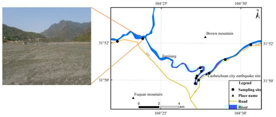
Figure 1.
Study area with a picture of the sampling site.
Furthermore, the study area is the severely damaged area of the Wenchuan earthquake, which took place in 2008, with a magnitude of Ms8.0. Since then, several debris flow disasters have happened on 20 August 2019, 11 July 2018, 28 July 2016, 6 July 2013, 17 August 2011, and 24 September 2008, resulting in a large number of houses destroyed, farmland flooded, and nearly 10,000 people left their homes.
2.2. Methods
As shown in Figure 2, we carried out the research according to the technical flow of “(i) research area and background data acquisition, (ii) parameter measurement experiments, (iii) model establishment, (iv) results”.
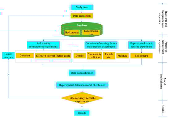
Figure 2.
Flowchart of cohesion hyperspectral detection model.
(1) Background data acquisition
We obtained the background data, such as geology, meteorology, land use, and high-resolution remote sensing data, such as Gaofen-2 (GF-2) remote sensing imagery. With a spatial resolution of 0.8 m in the panchromatic band, the Gaofen-2 satellite was launched on 19 August 2014, China. From it, the distribution of fine-grained sediments is extracted, and then the database of internally controlled factors for the stability of fine-grained sediments is established. GF-2 is one of the China High-resolution Earth Observation System (CHEOS) series of satellites. CHEOS was established as one of the sixteen major national science and technology projects under the strategic guidelines for the Medium and Long Term National Science and Technology Development Program (2006–2020). With the aim of building up a high-resolution Earth observation system based on satellites, stratospheric airships, and aircrafts, it will provide a global earth observation capability on hazards, agriculture, resource and environment monitoring, etc.
(2) Parameter measurement experiments
First, we made samples using ring knives according to the investigation standard of landslides, collapses, and debris flows (DZ/T 02161-2014) [27] and a technical guide for soil sampling (GB/T 36197-2018) [28]. No fine-grained sediments were present on the surface and small branches and small stones were cleared out; then, a ring knife was put into sediments vertically and pulled out when it was fully filled with soils; excess soils were cut out using a dull knife along the horizontal edge of the ring knife and, finally, a sample was made by putting the soils in the ring knife into a plastic bag.
Second, soil parameter measurement experiments were carried out according to the soil experiment specification (SL237-1999) [29]. The parameters include cohesion, effective internal friction angle, permeability coefficient, density, moisture, and particle size. The main steps of the parameter measurement were the following and more detailed information on these experiments can be found in [30]: ① cohesion, effective internal friction angle measurement. A model ZJ strain controlled direct shear apparatus was used to measure cohesion and effective internal friction angle. The main steps include sample preparation, adding shear normal stress σ of 50, 100, 200, and 300 kpa to obtain shear strength τ, then cohesion and effective internal friction angle can be calculated by displaying the measured 4 pairs of data in the coordinate system with σ as the horizontal axis and τ as the vertical axis. Cohesion is the intercept of the straight line, and the internal friction angle is the inclination angle of slope; ② permeability coefficient measurement. A TST-55 permeameter was used to measure permeability coefficient. The main steps include sample preparation, flowing water through the sample, and recording parameters, such as initial water head, starting time, and the end water head, then calculating the permeability coefficient according to Formula (1).
in which is the permeability coefficient at temperature T, a is the cross-sectional area of the variable head pipe (cm2), L is the height of the sample (cm), A is the cross-sectional area of the sample (cm2), t is the time (s), h1 is the starting water head (cm), and h2 is the ending water head (cm); ③ density measurement. An MDJ-300A solid densitometer was used to measure density. The main steps include sample preparation, weighing the sample as w g, then calculating density by ρ = w/v. ρ is the density and v is the sample volume of 600 mL; ④ moisture measurement. An electric heating constant temperature drying oven was used to measure moisture. The main steps include sample preparation and weighing as w1 g, drying samples for more than 8 h, weighing dried samples as w2 g, and then calculating moisture by ω = (w1 − w2)/w2. ω is the moisture; ⑤ particle size measurement. The Microtrac S3500 laser particle sizer was used to measure particle size. The main steps include setting the sample number and parameters on the instrument, particle size automatic measurement, saving data, and cleaning the pipeline.
Finally, a soil hyperspectral measurement experiment was carried out in the laboratory using the American ASD portable spectrometer. The main steps include fixing the 1000 Watt halogen lamp on a tripod with an approximately 20 cm distance to the sample, eliminating dark current, standardizing with a whiteboard, and then measuring the soil spectra. Each sample was measured 5 times, and the mean value was taken as the final spectrum.
(3) Model establishment
Cohesion sensitive band selection: backward elimination was applied when selecting sensitive bands by a multi-variate regression analysis method. Backward elimination is a variable selection procedure in which all variables are entered into the equation and then sequentially removed. The variable that has the smallest partial correlation with the dependent variable is considered first for removal. Once the first variable has been removed, the variable with the smallest partial correlation is considered next. The procedure stops when there are no variables in the equation that satisfy the removal criteria [12].
Based on cohesion and its sensitive bands, a cohesion hyperspectral detection model is established by using the least square multi-variate statistical analysis method.
The least square multi-variate statistical analysis method is a mathematical optimization technology. It finds the best matching function of data by minimizing the sum of squared errors.
Its basic principles are:
in which is a set of linearly independent functions, is the undetermined coefficient (k = 1, 2, ..., m), and the fitting criterion is to minimize the sum of the square distance between the measured value yi and the predicted value f(xi), which is also named as the least square criterion.
Let (x, y) be a pair of observations, and x = [x1, x2, …, xn]T ∈ Rn, y ∈ R. They satisfy the following functions:
in which w = [w1, w2, …, wn]T is an unknown parameter. In order to find the optimal estimate of the parameter w of , for a series of given datasets (xi, yi), the objective function can be solved as:
Parameters wi (I = 1, 2, …, n) can be determined when minimizing the value of the objective function.
(4) Results
After establishing the cohesion hyperspectral detection model, the accuracy of the model is checked. When the accuracy does not meet the requirements, it is necessary to analyze the causes and improve the model; otherwise, the model is finally output.
2.3. Data Acquisition and Processing
(1) Background data
We collected geological maps, meteorological and hydrological maps, topographic maps, traffic maps, and other maps of the study area to provide background data for this study.
We obtained high-resolution remote sensing data, such as GF-2, to extract the debris flow sediments and locate the sampling sites.
According to the national standard (GB/T 30319-2013) [31], a cohesion hyperspectral remote sensing database was established to save the background data, remote sensing images, experimental data, and results.
(2) Sample collection
As shown in Figure 1, from 19–25 March 2021, we took 200 samples using a ring knife. Each of which had a volume of 600 mL and a weight of about 1 kg. There are 11 sampling sites in total, and about 20 samples were taken at each site.
(3) Data acquisition
We carried out a shear strength measurement experiment on fine-grained sediments to obtain cohesion and effective internal friction angle, as well as experiments on cohesion influencing factors such as density, permeability coefficient, moisture, and particle size. Based on the above data, the correlation between cohesion and its influencing factors is established to discover the hyperspectral detection mechanism of fine-grained sediment cohesion in the study area [30].
(a) Shear strength measurement experiment
Soil shear strength refers to the ultimate capacity of soil to resist shear stress, including cohesion and effective internal friction angle. Effective internal friction angle is the internal friction between soil particles, mainly including the surface friction of soil particles and the bonding force between them. Their relationship can be expressed by
in which τ is the shear stress (kPa); σ is the normal stress (kPa); φ is the internal friction angle (kPa); and c is cohesion (kPa).
The main steps of measuring cohesion and effective internal friction angle can be found in Section 2.2 (2). The results of the experiment showed that the minimum soil cohesion was 13.95 kpa, and the maximum was 33.95 kpa, mostly concentrated within 20.35–26.75 kpa. Furthermore, the minimum effective internal friction angle was 16.16 and the maximum was 23.68, mostly concentrated within 18.98–21.8, belonging to silty soil [32].
(b) Particle size measurement experiment
The main steps of measuring particle size can be found in Section 2.2 (2) and the results of the experiment are shown in Figure 3. Φ calculated by –log(2,p) (p is the particle size with the unit of mm) is the horizontal axis and the cumulative probability is the vertical axis. From the results, we can see that the minimum particle size was 0.45 μm, and the maximum was 87.75 μm, mostly concentrated within 10–60 μm, belonging to silt particles. For Φ > 3, according to the classic particle size distribution curve, fine-grained sediments in the debris flow are mostly suspended materials with good separation.
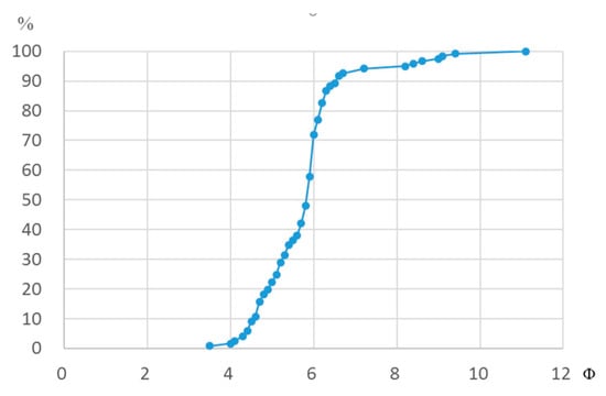
Figure 3.
Granulometric curve of fine-grained sediments.
(c) Density measurement experiment
The main steps of measuring density can be found in Section 2.2 (2) and the results showed that the minimum and maximum density were 1.34 g/mL and 1.73 g/mL, respectively, mostly concentrated within 1.34–1.54 g/mL, belonging to silt-sized particles.
(d) Permeability coefficient
The main steps of measuring permeability coefficient can be found in Section 2.2 (2) and the results showed that the minimum was 0.47 m/d, and the maximum was 2.85 m/d, mostly concentrated within 1.15–2.17 m/d, belonging to medium permeability.
(e) Moisture measurement experiment
The main steps of measuring moisture can be found in Section 2.2 (2) and the results showed that the minimum moisture was 4.01%, and the maximum was 30.69%, mostly concentrated within 4.01–12.02%.
(f) Spectral measurement experiment
The main steps of measuring spectra can be found in Section 2.2 (2) and the results showed that there are two spectral absorptions at about 1400 nm and 1900 nm. Furthermore, white noise in blue bands (350–450 nm) and short wave infrared bands (2350–2450 nm) commonly existed in the spectra.
(4) Data pre-processing
(a) Abnormal data elimination
As there are some abnormal cohesions, they were eliminated according to the principle of three times the standard deviation. After excluding abnormal samples, the number of modeling samples is 121.
(b) Spectral de-noising
Influenced by the instrument, the measured spectrum has white noise, especially in the blue bands and short wave infrared bands, which will seriously decrease the modeling accuracy. According to the frequency differences between noise and signal, we use Fourier transformation to eliminate spectral noises [33].
(c) Data standardization
Different data types often have different magnitudes due to their units. When there is a large magnitude difference between various parameters, the direct analysis with the original data will highlight the role of the parameters with higher values in the comprehensive analysis and weaken the role of the parameters with lower values. Therefore, in order to ensure the reliability of the results, it is necessary to standardize the original data to ensure that the processed data have an average of 0 and a standard deviation of 1 [30].
Data standardization can be expressed by
in which zij is the standardized value of variable xij, is the mean value of the variable xi, and si is the standard deviation of the variable xi.
3. Results and Analysis
3.1. Cohesion Influencing Factors
Shown in Table 1, in order to evaluate the cohesion influencing factors, the correlation coefficients between cohesion and effective internal friction angle, permeability coefficient, density, moisture, and particle size were calculated by SPSS v13.0 software.

Table 1.
Table of correlation coefficients between cohesion and its influencing factors.
It can be seen from Table 1 that, except for particle size, cohesion is correlated to effective internal friction angle, permeability coefficient, density, and moisture at the 0.01 significance level [23], whose scatter plots are shown in Figure 4. Cohesion is negatively correlated to the former two, with correlation coefficients of −0.664 and −0.557, respectively; while it is positively correlated to the latter two, with the correlation coefficients of 0.356 and 0.316, respectively.
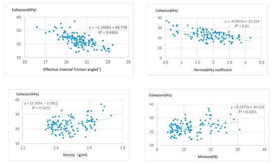
Figure 4.
Scatter plot of cohesion and its influencing factors.
3.2. Model
In order to discover the sensitive bands of cohesion and establish the model between them, first, the correlation coefficient was calculated to indicate bands related to cohesion; then, the least square multi-variate regression analysis method is used to establish a model between cohesion and the sensitive bands [12].
(1) Selection of sensitive bands
In order to find the bands closely related to cohesion, we calculated the correlation coefficients between the cohesion and each band’s reflectance; furthermore, in order to discover the bands sensitive to cohesion influencing factors, we also calculated the correlation coefficients between the effective internal friction angle, permeability coefficient, density, moisture, and the band reflectance. The results are shown in Figure 5.
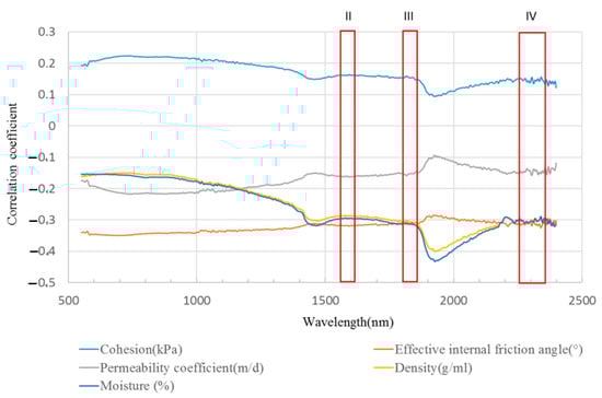
Figure 5.
Correlation coefficients between cohesion, effective internal friction angle, permeability coefficient, density, moisture, and band reflectance (I–IV indicate the highly correlated segments between spectra and cohesion).
From the cohesion coefficient curve in Figure 5, we can see that there are two reflectance absorption peaks: one is at about 1400 nm, and the other is at about 1900 nm. Cohesion sensitive bands would seem to indicate red (~700 nm) and near infrared (beyond 1000 nm) portions of the electromagnetic spectrum: (1) reflectance from 710 to 750 nm (I) is the highest correlated band to cohesion, when the wavelength is less than 1400 nm; (2) reflectance from 1578 to 1618 nm (II) is the second segment of highly correlated bands to cohesion when the wavelength is from 1400 to 1800 nm; (3) reflectance from 1804-1844 nm (III) is the third segment of highly correlated bands to cohesion, when the wavelength is from 1800 nm to 1900 nm; (4) and finally, reflectance from 2286–2363 nm (IV) is the fourth segment of highly correlated bands to cohesion, when the wavelength is greater than 1900 nm. Therefore, we utilize these four segments including 201 bands to select sensitive bands to cohesion. The backward elimination method in Section 2.2 (3) was applied to select six sensitive bands, including 750, 1578, 1835, 2301, 2305, and 2309 nm, from these four segments.
From Figure 5, we can see that correlation coefficients between the effective internal friction angle and the band reflectance are negative and whose absolute values are higher than those of others, such as permeability coefficient, density, and moisture in I–IV sensitive bands segments, indicating its high correlation with the sensitive bands in these four segments.
Then, from Figure 5, we can see that correlation coefficients between the permeability coefficient and the band reflectance are negative and whose absolute values are higher than those of density and moisture in the I segment, while they are lower in the II–IV segments, indicating that it is sensitive to band reflectance in the I segment.
Finally, from Figure 5, we can also see that correlation coefficients between the density and the band reflectance are negative and whose absolute values are less than those of permeability coefficient in the I segment, while they are higher in the II–IV segments, indicating that it is sensitive to band reflectance in the II–IV segments.
Correlation coefficients between moisture and the band reflectance have a similar tendency to density, indicating that it is also sensitive to band reflectance in the II–IV segments.
(2) Multi-variate regression analysis of cohesion and sensitive bands
The least square method is used to find the best matching function of the data by minimizing the squared summation of errors [34].
In this experiment, with cohesion as the dependent variable and the standardized spectral reflectance of six sensitive bands as the independent variables, a cohesion hyperspectral detection model is established as follows by the least square multi-variate statistical analysis method in Section 2.2 (3).
in which y is cohesion; x1 is the standardized reflectance at 750 nm; x2 is the normalized reflectance at 1578 nm; x3 is the normalized reflectance at 1835 nm; x4 is the normalized reflectance at 2301 nm; x5 is the normalized reflectance at 2305 nm; and x6 is the normalized reflectance at 2309 nm.
y = 22.7 + 10.36x1 − 37.32x2 + 42.57x3 − 30.34x4 + 56.15x5 − 40.42x6,
The fitting relationship between the measured and predicted cohesion is shown in Figure 6.
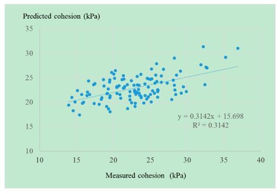
Figure 6.
Results of cohesion hyperspectral detection model.
As can be seen from Figure 6, the determination coefficient (R2) of the model is 0.3142, and whose correlation coefficient is 0.56; a t-test on each regression coefficient is shown in Table 2. The p value of each regression coefficient is less than 0.001, indicating that there is a significant correlation between cohesion and the six sensitive bands, and the established model has a good prediction ability.
Table 2.
t-test on the regression coefficients of the model.
After the sensitive band selection, correlation coefficients between each parameter and sensitive bands were calculated by the SPSS V13.0 software, as shown in Table 3.
Table 3.
Correlation coefficients between parameters and sensitive bands.
It can be seen from Table 3 that the band at 750 nm is significantly correlated to the effective internal friction angle at the significance level of 0.01, and correlated to cohesion and permeability coefficient at the significance level of 0.05; bands at 1578, 1835, 2301, 2305, and 2309 nm are significantly correlated to the effective internal friction angle, density, and moisture at the significance level of 0.01. This is mainly because these bands can better indicate the water content among I–IV highly correlated segments between spectra and cohesion (Figure 5). Density in this research is closely correlated to moisture with a correlation coefficient of 0.796 at the 0.01 significance level (Table 3). Therefore, moisture and density are correlated to these sensitive bands. In other words, these sensitive bands indicate cohesion influencing factors and its hyperspectral detection mechanism.
4. Discussion
Reasons for correlations between cohesion and its influencing factors are analyzed as follows, providing a theoretical basis for discovering the cohesion hyperspectral detection mechanism of fine-grained sediments in Beichuan debris flow.
(1) Force between soil particles makes cohesion negatively correlated to effective internal friction angle.
Cohesion is negatively correlated to effective internal friction angle at the significance level of 0.01. This is mainly because effective internal friction angle depends on the friction resistance and bonding force between soil particles. Therefore, the more edges and coarser and denser the soil particle surface, the greater the effective internal friction angle becomes; however, the coarser the surface is, the more edges and corners there are, resulting in a larger distance between particles and thus weakening of the gravitational forces between soil particles and lower cohesion.
(2) Distance between soil particles makes cohesion negatively correlated to permeability coefficient, while positively correlated to density.
Cohesion is negatively correlated to permeability coefficient at the 0.01 significance level. This is mainly because the permeability coefficient mainly reflects the size, number, and connectivity of soil pores [35]. The larger the permeability coefficient is, the greater the distance between soil particles is, and thus making the attraction between soil particles lower and the cohesion weakened.
However, cohesion is positively correlated to density at the 0.01 significance level. This is mainly because the greater the density is, the shorter the distance between particles becomes, the stronger the attraction between soil particles is, and the greater the cohesion between soil particles becomes [17].
(3) Water film makes cohesion positively correlated to moisture in unsaturated soil samples, while negatively in saturated ones.
Cohesion is positively correlated to moisture at the 0.01 significance level. Previous research showed that cohesion was positively correlated to moisture in unsaturated samples, while negatively in saturated ones [19]. This is mainly because when soil is dry, cohesion is mainly caused by the molecular gravity of soil particles themselves; when soil becomes wet, the molecular gravity between soil particles acts through the water film between soil particles, forming the mutual attraction among particles–water–particles due to the clay content in soil. The silty soil particle surface is very small and, when there is a small amount of water, the water film increases the contact area and thus increases the cohesion. However, when the soil is saturated, with the increase in moisture, the water film distance between soil particles becomes longer and thus decreases the cohesion [19].
5. Conclusions
In order to establish a hyperspectral remote sensing detection model for the cohesion of fine-grained sediments in debris flow, we designed experiments to measure soil cohesion and its influencing factors, including effective internal friction angle, permeability coefficient, density, and moisture. We also carried out a soil hyperspectral measurement experiment to select cohesion sensitive bands and establish a model between cohesion and these bands, with conclusions as follows.
(1) Six cohesion hyperspectral sensitive bands are found to provide a scientific basis for rapid detection of the fine-grained sediments’ stability in large areas.
Taking cohesion as the dependent variable and normalized spectral reflectance as independent variables, a model was established by the multi-variate regression analysis method in SPSS v13.0 software. The backward elimination method was used to select sensitive bands. According to the coefficient of determination (R2), t-test and p values, six sensitive bands for cohesion hyperspectral detection are found to be 750 nm, 1578 nm, 1835 nm, 2301 nm, 2305 nm, and 2309 nm.
These bands can be used in the future to quickly acquire soil cohesion by hyperspectral remote sensing. As cohesion is one of the internally controlled factors of soil stability, this finding thus provides a scientific basis for rapid detection of the fine-grained sediments’ stability in large areas.
(2) A cohesion hyperspectral remote sensing detection model for fine-grained sediments in Beichuan debris flow is established to provide a scientific basis for debris flow early warning.
Using the least square multi-variate regression analysis method, a model between cohesion and its sensitive bands is established with a correlation coefficient of 0.56. The results showed that there was a multi-variate linear correlation between cohesion and sensitive bands; the t-test results of each regression coefficient showed that the p values of each regression coefficient were less than 0.001, indicating that there was a significant correlation between cohesion and the six sensitive bands.
Debris flow early warning needs to quickly detect the stability of these fine-grained sediments which is one of the factors controlling disaster scales. Cohesion reflects the strain capacity of soil to resist external stress, and is closely related to the stability. Although cohesion varies with water content, we can quickly find its value with the model when the fine-grained sediments on the surface are in their natural state. Then, dangerous areas can be circled out by the early warning system according to the value of soil stability estimated by cohesion. In other words, less stability indicates higher danger.
(3) The cohesion hyperspectral detection mechanism of fine-grained sediments in Beichuan debris flow is discovered.
The results showed that cohesion was correlated to the effective internal friction angle, permeability coefficient, density, and moisture at the significance level of 0.01. Cohesion was negatively correlated to the former two factors, and positively correlated to the latter two; the band at 750 nm indicated the characteristics of cohesion, effective internal friction angle, and permeability coefficient, while the other five bands, 1578 nm, 1835 nm, 2301 nm, 2305 nm, and 2309 nm, indicated the characteristics of effective internal friction angle, density, and moisture. Therefore, these hyperspectral sensitive bands indicated the cohesion hyperspectral remote sensing detection mechanism of fine-grained sediments in Beichuan debris flow.
Author Contributions
Conceptualization, Q.W. and J.X.; methodology, Q.W., J.X., J.Y., and P.L.; validation, Q.W., J.X., and P.L.; formal analysis, Q.W. and J.X.; investigation, Q.W., J.X., P.L., D.C., and W.X.; data curation, J.X., J.Y., and P.L.; writing—original draft preparation, Q.W., J.X., and J.Y.; writing—review and editing, Q.W.; visualization, D.C.; supervision, W.X.; project administration, Q.W.; funding acquisition, Q.W. All authors have read and agreed to the published version of the manuscript.
Funding
This work was supported in part by the National Natural Science Foundation of China (No. 42071312), in part by the Special Project of Strategic Leading Science and Technology of the Chinese Academy of Sciences (No. XDA19090139), in part by the Hainan Hundred Special Project (No. 31, JTT [2018]), and in part by the National Key R&D Program of China (No. 2021YFB3900503).
Institutional Review Board Statement
Not applicable.
Informed Consent Statement
Not applicable.
Data Availability Statement
Not applicable.
Conflicts of Interest
The authors declare no conflict of interest.
References
- Liu, P.; Wei, Y.; Wang, Q.; Xie, J.; Chen, Y.; Li, Z.; Zhou, H. A research on landslides automatic extraction model based on the improved Mask R-CNN. ISPRS Int. J. Geo-Inf. 2021, 10, 168. [Google Scholar] [CrossRef]
- Xiao, J. The Emergency Management Department of China Announced the National Top Ten Disasters in 2019 [ER/OL]. 2020. Available online: https://society.people.com.cn/n1/2020/0112/c1008-31544517.html (accessed on 2 January 2022).
- Tang, C.; Liang, J. Study on characteristics of 9.24 rainstorm and debris flow in Beichuan, Wenchuan earthquake area. J. Eng. Geol. 2008, 16, 751–758. [Google Scholar]
- Wu, Q.; Xu, L.; Zhou, K.; Liu, Z. Starting analysis of loose sediments of gully debris flow. J. Nat. Disasters 2015, 24, 89–97. [Google Scholar]
- Miao, Q.; Yang, D.; Yang, H.; Li, Z. Establishing a rainfall threshold for flash flood warnings in China’s mountainous areas based on a distributed hydrological model. J. Hydrol. 2016, 541, 371–386. [Google Scholar] [CrossRef]
- Xie, J.; Wang, M.; Liu, K.; Coulthard, T.J. Modeling sediment movement and channel response to rainfall variability after a major earthquake. Geomorphology 2018, 320, 18–32. [Google Scholar] [CrossRef]
- Ma, M. Stability analysis of high slope of accumulation at the outlet of pressure flood discharge and sediment discharge tunnel of Jiudianxia Water Control Project. Water Conserv. Plan. Des. 2019, 4, 64–67. [Google Scholar]
- Tang, M.; Xu, Q.; Li, J.; Luo, J.; Kuang, Y. An experimental study of the failure mechanism of shallow landslides after earthquake triggered by rainfall. Hydrogeol. Eng. Geol. 2016, 43, 128–135. [Google Scholar]
- Hürlimann, M.; Coviello, V.; Bel, C.; Guo, X.; Berti, M.; Graf, C.; Hübl, J.; Miyata, S.; Smith, J.B.; Yin, H. Debris-flow monitoring and warning: Review and examples. Earth-Sci. Rev. 2019, 199, 102981. [Google Scholar] [CrossRef]
- Langat, P.K.; Kumar, L.; Koech, R. Monitoring river channel dynamics using remote sensing and GIS techniques. Geomorphology 2019, 325, 92–102. [Google Scholar] [CrossRef]
- AfiqHarun, M.; Aminuddin, A.; Mohammadpour, G.; WengChan, N. Stable channel analysis with sediment transport for rivers in Malaysia: A case study of the Muda, Kurau, and Langat rivers. Int. J. Sediment Res. 2020, 35, 455–466. [Google Scholar] [CrossRef]
- Wang, Q.; Wei, Y.; Chen, Y.; Lin, Q. Hyperspectral soil dispersion model for the source region of the Zhouqu debris flow, Gansu, China. IEEE J. Sel. Top. Appl. Earth Obs. Remote Sens. 2016, 9, 876–883. [Google Scholar] [CrossRef]
- Hu, W.; Scaringi, G.; Xu, Q.; Pei, Z.; van Asch, T.W.J.; Hicher, P. Sensitivity of the initiation and runout of flow slides in loose granular sediments to the content of small particles-An insight from flume tests. Eng. Geol. 2017, 231, 34–44. [Google Scholar] [CrossRef]
- Fan, R.L.; Zhang, L.M.; Wang, H.J.; Fan, X.M. Evolution of debris flow activities in Gaojiagou Ravine during 2008-2016 after the Wenchuan earthquake. Eng. Geol. 2018, 235, 1–10. [Google Scholar] [CrossRef]
- Khezri, N.; Mohamad, H.; HajiHassani, M.; Fatahi, B. The stability of shallow circular tunnels in soil considering variations in cohesion with depth. Tunn. Undergr. Space Technol. 2015, 49, 230–240. [Google Scholar] [CrossRef]
- Sun, J.; Hong, B.; Li, J. Sensitivity analysis on stability of embankment slope based on cohesion and friction angle. J. Resour. Archit. Eng. 2013, 11, 99–104. [Google Scholar]
- Zhang, K.; Li, M.; Yang, B. Research on effect of water content and dry density on shear strength of remolded loess. J. Anhui Univ. Sci. Technol. (Nat. Sci.) 2016, 36, 74–79. [Google Scholar]
- Zhou, C.; Cheng, Y.; Wang, Y.; Wang, Q.; Fu, M. Study on influencing factors of shear strength parameters of compacted loess. J. Disaster Prev. Mitig. Eng. 2018, 38, 258–264. [Google Scholar]
- Yan, M. The Effect of Water Content on Apparent Cohesion of Sand and Its Engineering Application. Master’s Thesis, Chang’an University, Xi’an, China, 2018. [Google Scholar]
- Tian, W.; Tong, F.; Liu, C.; Zhao, Y. Shear strength model of red soil considering influence of saturation and its application. Water Resour. Power 2018, 36, 124–127. [Google Scholar]
- Song, Y.; Xu, X.; Yang, S.; Gao, M. Influence of water content on shear strength of granite residual soil in Huangdao area. J. Shandong Univ. Sci. Technol. (Nat. Sci.) 2019, 38, 33–40. [Google Scholar]
- Dong, S.; Wang, H.; Li, J.; Ma, F.; Bai, X. Effects of water content and compaction degree on mechanical characteristics of compacted silty soil. J. Guangxi Univ. (Nat. Sci. Ed.) 2020, 45, 978–985. [Google Scholar]
- Wang, C.; Sun, Z.; Bian, H.; Lu, X.; Qiu, X. Significance analysis of factors affecting the cohesion of silty clay. J. Shandong Agric. Univ. (Nat. Sci. Ed.) 2020, 51, 646–650. [Google Scholar]
- Tang, C.; Borden, R.H.; Gabr, M.A. Model applicability for prediction of residual soil apparent cohesion. Transp. Geotech. 2019, 19, 44–53. [Google Scholar] [CrossRef]
- Kim, Y.; Satyanaga, A.; Rahardjo, H.; Park, H.; Sham, A.W.L. Estimation of effective cohesion using artificial neural networks based on index soil properties: A Singapore case. Eng. Geol. 2021, 289, 106163. [Google Scholar] [CrossRef]
- Saygin, S.D.; Arı, F.; Temiz, Ç.; Arslan, S.; Ünal, M.A.; Erpul, G. Analysis of soil cohesion by fluidized bed methodology using integrable differential pressure sensors for a wide range of soil textures. Comput. Electron. Agric. 2021, 191, 106525. [Google Scholar] [CrossRef]
- DZ/T 02161-2014; Geological and Mineral Industry Standard of the People’s Republic of China: Code for Investigation of Landslide, Collapse and Debris Flow Disasters 1:50,000. China Standards Press: Beijing, China, 2015.
- GB/T 36197-2018; National Standard of the People’s Republic of China: Technical Guide for Soil Sampling of Soil Quality. China National Standardization Administration Committee: Beijing, China, 2018.
- SL237-1999; National Standard of the People’s Republic of China: Geotechnical Test Code. China Water Resources and Hydropower Press: Beijing, China, 1999.
- Wang, Q.; Xie, J.; Yang, J.; Liu, P.; Chang, D.; Xu, W. Research on permeability coefficient of fine sediments in debris-flow gullies, southwestern China. Soil Syst. 2022, 6, 29. [Google Scholar] [CrossRef]
- GB/T 30319-2013; National Standard of the People’s Republic of China: Basic Provisions for Basic Geographic Information Database. China National Standardization Administration Committee: Beijing, China, 2013.
- Sun, X.; Wang, D. Analysis of cohesion value of soil. Liaoning Build. Mater. 2010, 3, 39–42. [Google Scholar]
- Chen, T.; Wang, Y.; Pu, X. The application of Fourier transform in the noise smoothing of weak Raman spectrum. J. Yunnan Univ. 2005, 27, 509–513. [Google Scholar]
- Wu, B.; Wang, X.; Zhang, L. Iterative abstraction of endmember based on total least square for mixture pixel decomposition. Geomat. Inf. Sci. Wuhan Univ. 2008, 33, 457–461. [Google Scholar]
- Liu, Y. Study on test method of permeability coefficient of cohesion less coarse-grained soil in hydraulic engineering. Shanxi Water Conserv. 2020, 12, 211–213. [Google Scholar]
Publisher’s Note: MDPI stays neutral with regard to jurisdictional claims in published maps and institutional affiliations. |
© 2022 by the authors. Licensee MDPI, Basel, Switzerland. This article is an open access article distributed under the terms and conditions of the Creative Commons Attribution (CC BY) license (https://creativecommons.org/licenses/by/4.0/).