
Integrated Modelling Approaches for Sustainable Agri-Economic Growth and Environmental Improvement: Examples from Greece, Canada and Ireland


Abstract
:1. Introduction
2. Study Areas
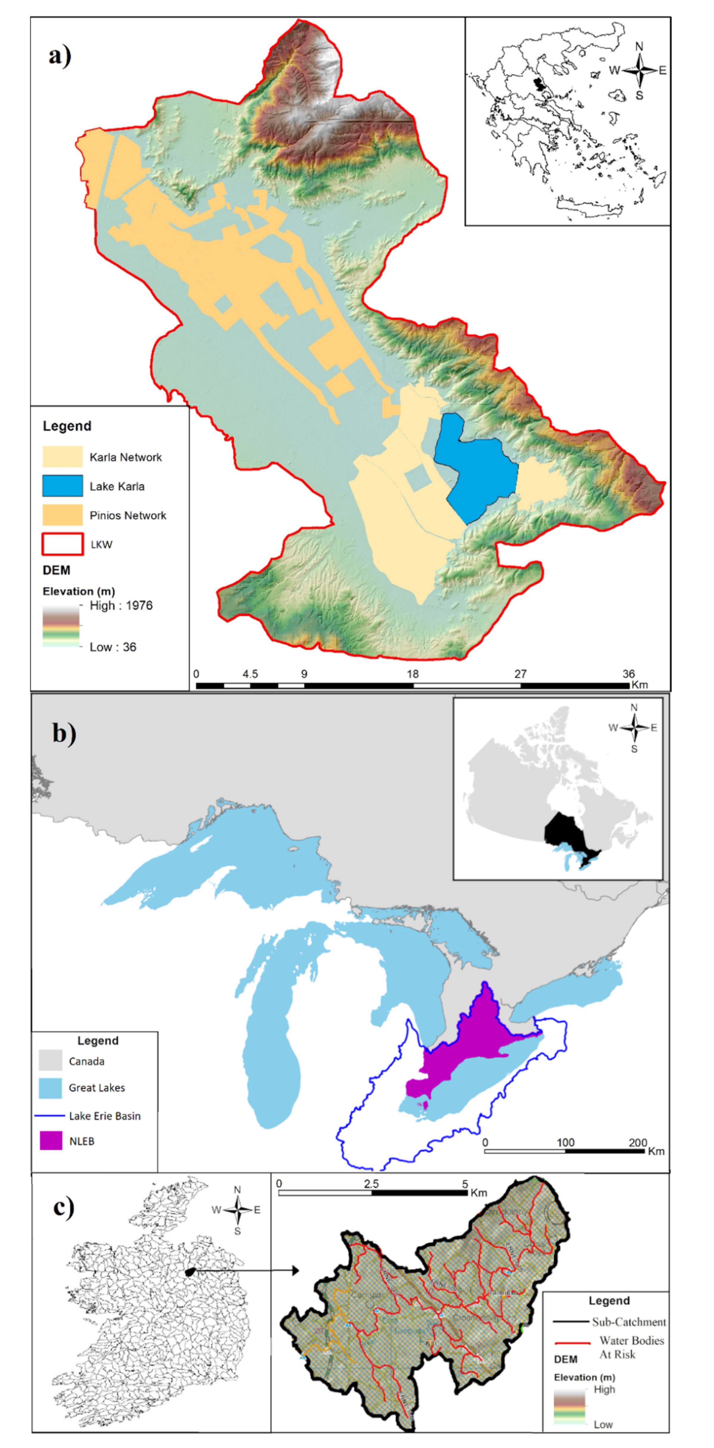
2.1. Lake Karla Watershed (LKW), Greece
2.2. Northern Lake Erie Basin (NLEB), Ontario, Canada
2.3. Erne Sub-Catchment Area (ESCA), Ireland
3. Methodology
3.1. Linear, Non-Linear and Goal Programming
3.2. The LKW Model
3.3. The NLEB Model
3.4. The ESCA Model
4. Results
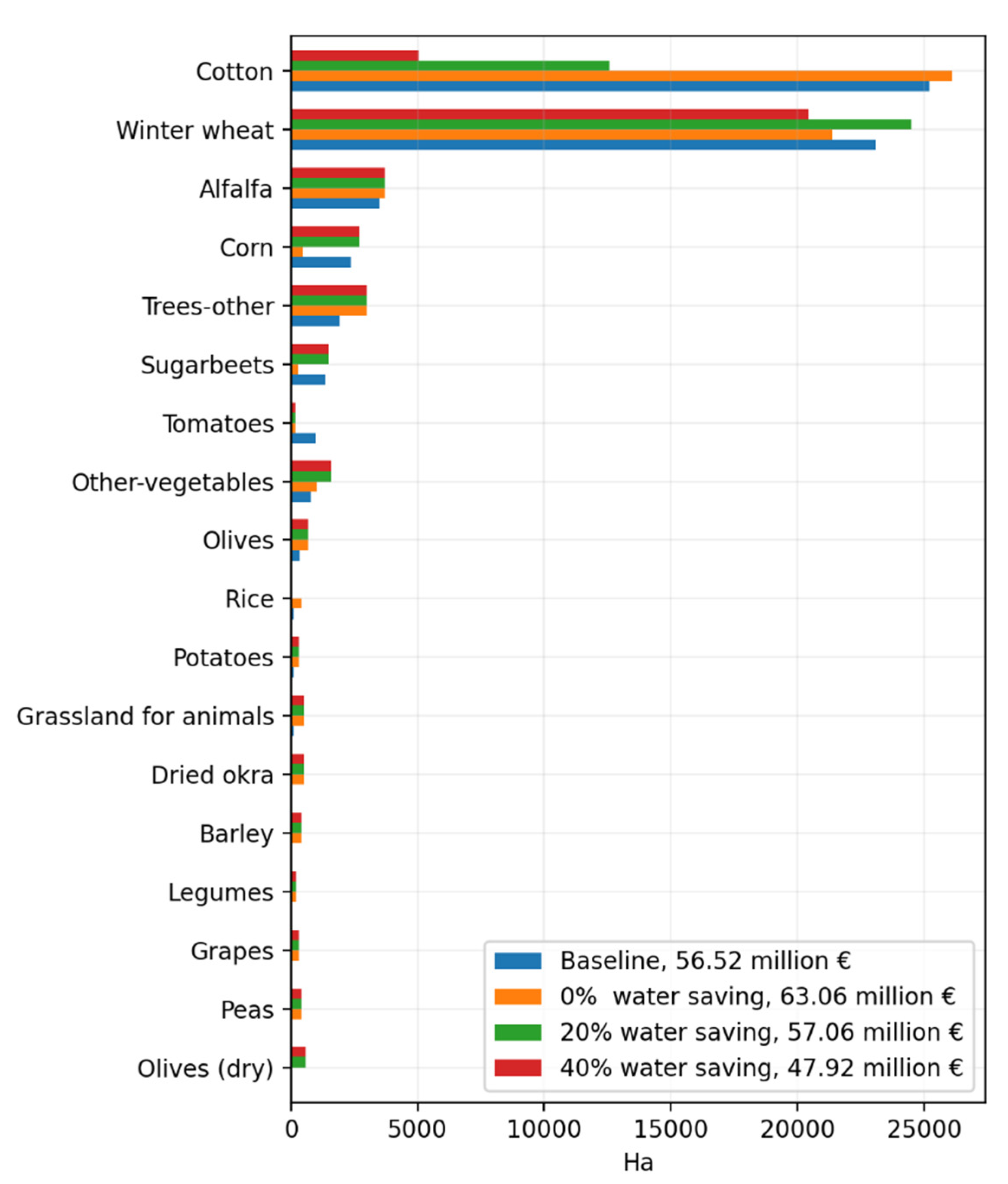
4.1. LKW Model
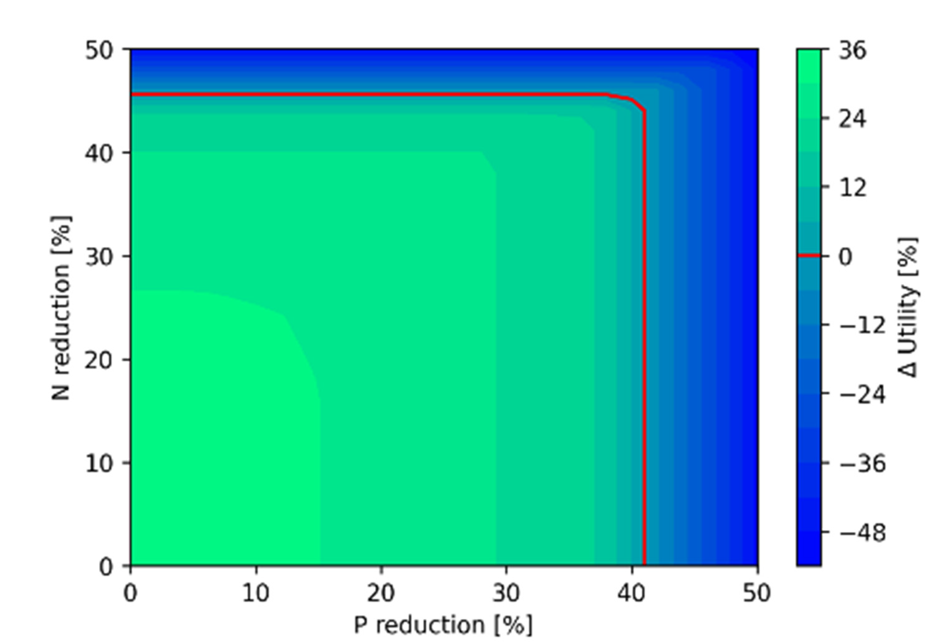
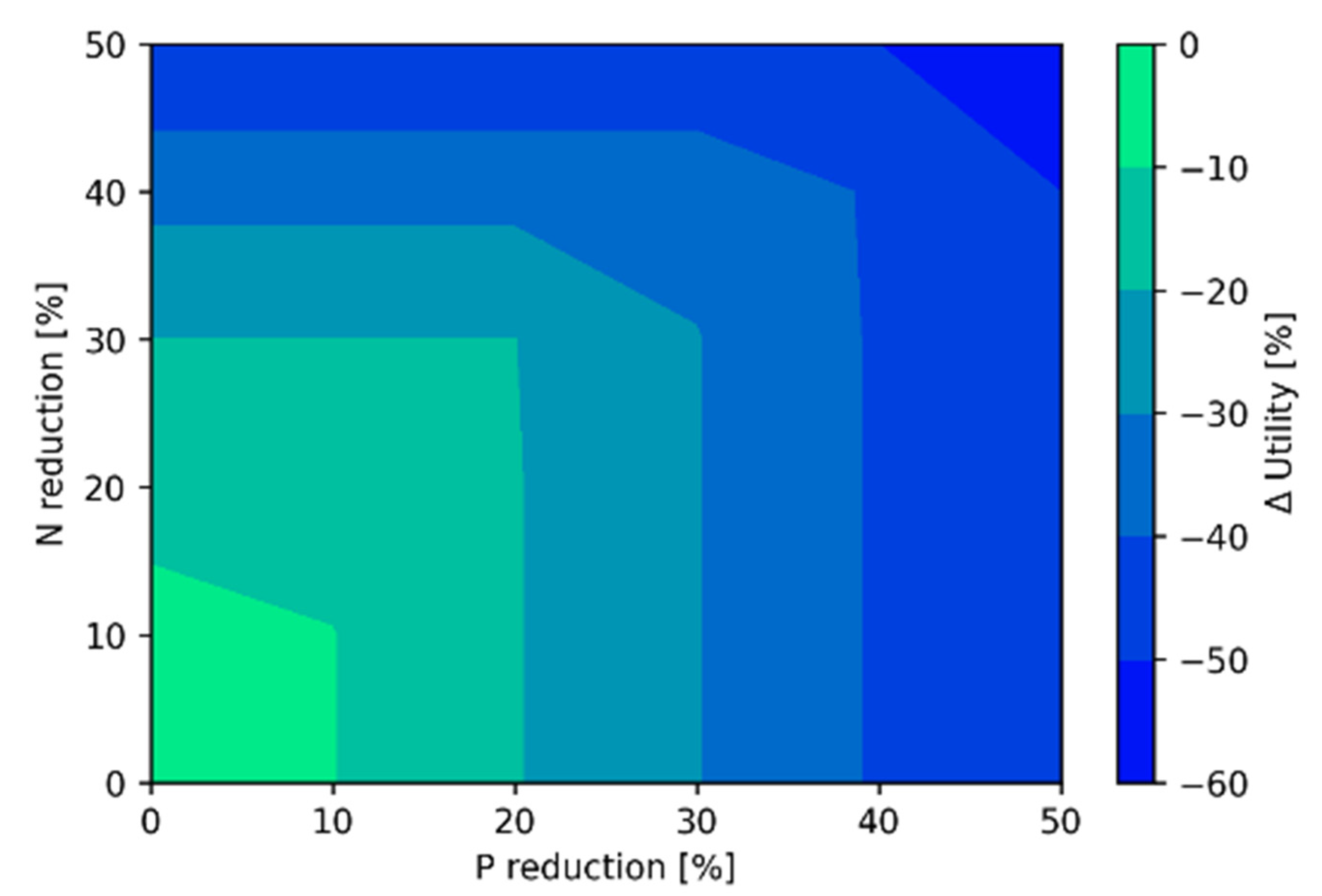
4.2. NLEB Model
4.3. ESCA Model
- Scen. A: Extremely environmentalist (only caring to have zero emissions and ignoring the other goals).
- Scen. B: Intensive farmer (only caring about maximum sales and profits, and then reduced costs while ignoring all the rest).
- Scen. C: A balanced penalization, representing the ‘middle solution’ between the first two scenarios.

| Deviations Penalized | Scen. A | Scen. B | Scen. C |
|---|---|---|---|
| Deficit of beef sales () | 0.0 | 1.0 | 0.5 |
| Deficit of dairy sales () | 0.0 | 1.0 | 0.5 |
| Deficit of poultry sales () | 0.0 | 1.0 | 0.5 |
| Exceedance of costs—budget () | 0.0 | 0.1 | 0.0 |
| Exceedance of P emissions () | 1.0 | 0.0 | 0.5 |
| Exceedance of C emissions () | 1.0 | 0.0 | 0.5 |
| Exceedance of organic fertiliser () | 1.0 | 0.0 | 0.5 |
| Deficit of organic fertiliser () | 0.0 | 0.0 | 0.0 |
| Exceedance of beef production () | 0.01 | 0.0 | 0.005 |
| Deficit of beef production () | 0.01 | 0.0 | 0.005 |
| Exceedance of dairy production () | 0.01 | 0.0 | 0.005 |
| Deficit of dairy production () | 0.01 | 0.0 | 0.005 |
| Exceedance of poultry production () | 0.01 | 0.0 | 0.005 |
| Deficit of poultry production () | 0.01 | 0.0 | 0.005 |
| Water deficits () | 0.05 | 0.0 | 0.05 |
5. Comparability, Limitations and Future Research
6. Concluding Remarks
Supplementary Materials
Author Contributions
Funding
Data Availability Statement
Code Availability
Conflicts of Interest
| 1 | In every model the variables and constraints used can be modified to better tailor them for similar problems, depending the case and the data availability. |
References
- Zhang, L.; Yan, C.; Guo, Q.; Zhang, J.; Ruiz-Menjivar, J. The Impact of Agricultural Chemical Inputs on Environment: Global Evidence from Informetrics Analysis and Visualization. Int. J. Low-Carbon Technol. 2018, 13, 338–352. [Google Scholar] [CrossRef]
- Arias, M.A.; Ibáñez, A.M.; Zambrano, A. Agricultural Production amid Conflict: Separating the Effects of Conflict into Shocks and Uncertainty. World Dev. 2019, 119, 165–184. [Google Scholar] [CrossRef]
- Xia, Y.; Zhang, M.; Tsang, D.C.W.; Geng, N.; Lu, D.; Zhu, L.; Igalavithana, A.D.; Dissanayake, P.D.; Rinklebe, J.; Yang, X.; et al. Recent Advances in Control Technologies for Non-Point Source Pollution with Nitrogen and Phosphorous from Agricultural Runoff: Current Practices and Future Prospects. Appl. Biol. Chem. 2020, 63, 8. [Google Scholar] [CrossRef]
- Fernandes, A.C.P.; Sanches Fernandes, L.F.; Moura, J.P.; Cortes, R.M.V.; Pacheco, F.A.L. A Structural Equation Model to Predict Macroinvertebrate-Based Ecological Status in Catchments Influenced by Anthropogenic Pressures. Sci. Total Environ. 2019, 681, 242–257. [Google Scholar] [CrossRef]
- Knox, J.W.; Haro-Monteagudo, D.; Hess, T.M.; Morris, J. Identifying Trade-Offs and Reconciling Competing Demands for Water: Integrating Agriculture into a Robust Decision-Making Framework. Earths Future 2018, 6, 1457–1470. [Google Scholar] [CrossRef]
- Candemir, A.; Duvaleix, S.; Latruffe, L. Agricultural Cooperatives and Farm Sustainability—A Literature Review. J. Econ. Surv. 2021, 35, 1118–1144. [Google Scholar] [CrossRef]
- Porse, E.; Mika, K.B.; Litvak, E.; Manago, K.F.; Hogue, T.S.; Gold, M.; Pataki, D.E.; Pincetl, S. The Economic Value of Local Water Supplies in Los Angeles. Nat. Sustain. 2018, 1, 289–297. [Google Scholar] [CrossRef]
- Hashmi, A.H.A.; Ahmed, S.A.S.; Hassan, I.H.I. Optimizing Pakistan’s Water Economy Using Hydro-Economic Modeling: Optimizing Pakistan’s Water Economy Using Hydro-Economic Modeling. J. Bus. Econ. 2019, 11, 111–124. [Google Scholar]
- Alamanos, A. Simple Hydro-Economic Tools for Supporting Small Water Supply Agencies on Sustainable Irrigation Water Management. Water Supply 2021, 22, 1810–1819. [Google Scholar] [CrossRef]
- Hatamkhani, A.; Moridi, A. Optimal Development of Agricultural Sectors in the Basin Based on Economic Efficiency and Social Equality. Water Resour. Manag. 2021, 35, 917–932. [Google Scholar] [CrossRef]
- Alamanos, A.; Latinopoulos, D.; Xenarios, S.; Tziatzios, G.; Mylopoulos, N.; Loukas, A. Combining Hydro-Economic and Water Quality Modeling for Optimal Management of a Degraded Watershed. J. Hydroinformatics 2019, 21, 1118–1129. [Google Scholar] [CrossRef] [Green Version]
- Loucks, D.; van Beek, E. Water Resource Systems Planning and Management; Springer International Publishing: Berlin/Heidelberg, Germany, 2017; ISBN 978-3-319-44234-1. [Google Scholar]
- Peres, D.J.; Cancelliere, A. Environmental Flow Assessment Based on Different Metrics of Hydrological Alteration. Water Resour. Manag. 2016, 30, 5799–5817. [Google Scholar] [CrossRef]
- Loukas, A.; Mylopoulos, N.; Vasiliades, L. A Modeling System for the Evaluation of Water Resources Management Strategies in Thessaly, Greece. Water Resour. Manag. 2007, 21, 1673–1702. [Google Scholar] [CrossRef]
- Kairis, O.; Karamanos, A.; Voloudakis, D.; Kapsomenakis, J.; Aratzioglou, C.; Zerefos, C.; Kosmas, C. Identifying Degraded and Sensitive to Desertification Agricultural Soils in Thessaly, Greece, under Simulated Future Climate Scenarios. Land 2022, 11, 395. [Google Scholar] [CrossRef]
- Sargentis, G.-F.; Siamparina, P.; Sakki, G.-K.; Efstratiadis, A.; Chiotinis, M.; Koutsoyiannis, D. Agricultural Land or Photovoltaic Parks? The Water–Energy–Food Nexus and Land Development Perspectives in the Thessaly Plain, Greece. Sustainability 2021, 13, 8935. [Google Scholar] [CrossRef]
- Charizopoulos, N.; Zagana, E.; Psilovikos, A. Assessment of Natural and Anthropogenic Impacts in Groundwater, Utilizing Multivariate Statistical Analysis and Inverse Distance Weighted Interpolation Modeling: The Case of a Scopia Basin (Central Greece). Environ. Earth Sci. 2018, 77, 380. [Google Scholar] [CrossRef]
- Sidiropoulos, P.; Mylopoulos, N.; Loukas, A. Optimal Management of an Overexploited Aquifer under Climate Change: The Lake Karla Case. Water Resour. Manag. 2013, 27, 1635–1649. [Google Scholar] [CrossRef]
- Panagopoulos, Y.; Makropoulos, C.; Kossida, M.; Mimikou, M. Optimal Implementation of Irrigation Practices: Cost-Effective Desertification Action Plan for the Pinios Basin. J. Water Resour. Plan. Manag. 2014, 140, 05014005. [Google Scholar] [CrossRef]
- Alamanos, A.; Xenarios, S.; Mylopoulos, N.; Stålnacke, P. Integrated Water Resources Management in Agro-Economy Using Linear Programming: The Case of Lake Karla Basin, Greece. Eur. Water 2017, 60, 41–47. [Google Scholar]
- Watson, S.B.; Miller, C.; Arhonditsis, G.; Boyer, G.L.; Carmichael, W.; Charlton, M.N.; Confesor, R.; Depew, D.C.; Höök, T.O.; Ludsin, S.A.; et al. The Re-Eutrophication of Lake Erie: Harmful Algal Blooms and Hypoxia. Harmful Algae 2016, 56, 44–66. [Google Scholar] [CrossRef]
- Ontario Ministry of Agriculture, Food and Rural Affairs (OMAFRA). Assessing the Economic Value of Protecting the Great Lakes Ecosystems. Available online: http://omafra.gov.on.ca/english/ (accessed on 21 July 2022).
- EPA Canada Canada-Ontario Lake Erie Action Plan. Available online: https://www.canada.ca/en/environment-climate-change/services/great-lakes-protection/action-plan-reduce-phosphorus-lake-erie.html (accessed on 21 July 2022).
- Alamanos, A.; Garcia, J.A. Balancing Phosphorus Runoff Reduction and Farmers’ Utility: An Optimization for Lake Erie. In Proceedings of the International Association of Great Lakes Research (IAGLR), 64th Annual Conference on Great Lakes Research, Online, 17–21 May 2021. [Google Scholar]
- Agro, E.; Zheng, Y. Controlled-Release Fertilizer Application Rates for Container Nursery Crop Production in Southwestern Ontario, Canada. HortScience 2014, 49, 1414–1423. [Google Scholar] [CrossRef]
- Hanief, A.; Laursen, A.E. Meeting Updated Phosphorus Reduction Goals by Applying Best Management Practices in the Grand River Watershed, Southern Ontario. Ecol. Eng. 2019, 130, 169–175. [Google Scholar] [CrossRef]
- Adhami, M.; Sadeghi, S.H.; Duttmann, R.; Sheikhmohammady, M. Changes in Watershed Hydrological Behavior Due to Land Use Comanagement Scenarios. J. Hydrol. 2019, 577, 124001. [Google Scholar] [CrossRef]
- Liu, J.; Elliott, J.A.; Wilson, H.F.; Macrae, M.L.; Baulch, H.M.; Lobb, D.A. Phosphorus Runoff from Canadian Agricultural Land: A Cross-Region Synthesis of Edge-of-Field Results. Agric. Water Manag. 2021, 255, 107030. [Google Scholar] [CrossRef]
- Jeffrey, S.R.; Gibson, R.R.; Faminow, M.D. Nearly Optimal Linear Programming as a Guide to Agricultural Planning. Agric. Econ. 1992, 8, 1–19. [Google Scholar] [CrossRef]
- Liu, Y.; Shen, H.; Yang, W.; Yang, J. Optimization of Agricultural BMPs Using a Parallel Computing Based Multi-Objective Optimization Algorithm. Environ. Resour. Res. 2013, 1, 39–50. [Google Scholar] [CrossRef]
- Sharpley, A.; Jarvie, H.P.; Buda, A.; May, L.; Spears, B.; Kleinman, P. Phosphorus Legacy: Overcoming the Effects of Past Management Practices to Mitigate Future Water Quality Impairment. J. Environ. Qual. 2013, 42, 1308–1326. [Google Scholar] [CrossRef]
- Chiodi, A.; Donnellan, T.; Breen, J.; Deane, P.; Hanrahan, K.; Gargiulo, M.; Gallachóir, B.P.Ó. Integrating Agriculture and Energy to Assess GHG Emissions Reduction: A Methodological Approach. Clim. Policy 2016, 16, 215–236. [Google Scholar] [CrossRef]
- Conroy, E.; Turner, J.N.; Rymszewicz, A.; O’Sullivan, J.J.; Bruen, M.; Lawler, D.; Lally, H.; Kelly-Quinn, M. The Impact of Cattle Access on Ecological Water Quality in Streams: Examples from Agricultural Catchments within Ireland. Sci. Total Environ. 2016, 547, 17–29. [Google Scholar] [CrossRef]
- Nasr, A.; Bruen, M.; Jordan, P.; Moles, R.; Kiely, G.; Byrne, P. A Comparison of SWAT, HSPF and SHETRAN/GOPC for Modelling Phosphorus Export from Three Catchments in Ireland. Water Res. 2007, 41, 1065–1073. [Google Scholar] [CrossRef]
- Irish Water National Water Utility, Irish Water. Available online: https://www.water.ie/ (accessed on 21 July 2022).
- NFGWS. Available online: https://nfgws.ie/ (accessed on 21 July 2022).
- EPA. Erne Catchment Assessment 2010–2015 (HA 36); Catchment Science & Management Unit: Dublin, Ireland, 2018; p. 54. [Google Scholar]
- EPA. 3rd Cycle Draft Erne Catchment Report (HA 36); Catchment Science & Management Unit: Dublin, Ireland, 2021; p. 57. [Google Scholar]
- Hayward, J.; Foy, R.H.; Gibson, C.E. Nitrogen and Phosphorus Budgets in the Erne System, 1974–1989. Biol. Environ. Proc. R. Ir. Acad. 1993, 93B, 33–44. [Google Scholar]
- Catchments Catchments.Ie. Available online: https://www.catchments.ie/ (accessed on 21 July 2022).
- Teagasc Agriculture and Food Development Authority. The Impact of Nitrogen Management Strategies within Grass Based Dairy Systems | Agriculture and Food Development Authority. Available online: https://www.teagasc.ie/ (accessed on 21 July 2022).
- Breen, M.; Murphy, M.D.; Upton, J. Development of a Dairy Multi-Objective Optimization (DAIRYMOO) Method for Economic and Environmental Optimization of Dairy Farms. Appl. Energy 2019, 242, 1697–1711. [Google Scholar] [CrossRef]
- Charnes, A.; Cooper, W. Management Models and Industrial Applications of Linear Programming, 1st ed.; John Wiley: New York, NY, USA, 1961. [Google Scholar]
- Alamanos, A.; Koundouri, P.; Papadaki, L.; Pliakou, T. A System Innovation Approach for Science-Stakeholder Interface: Theory and Application to Water-Land-Food-Energy Nexus. Front. Water 2022, 3, 744773. [Google Scholar] [CrossRef]
- Wurtsbaugh, W.A.; Paerl, H.W.; Dodds, W.K. Nutrients, Eutrophication and Harmful Algal Blooms along the Freshwater to Marine Continuum. WIREs Water 2019, 6, e1373. [Google Scholar] [CrossRef]
- Riley, W.D.; Potter, E.C.E.; Biggs, J.; Collins, A.L.; Jarvie, H.P.; Jones, J.I.; Kelly-Quinn, M.; Ormerod, S.J.; Sear, D.A.; Wilby, R.L.; et al. Small Water Bodies in Great Britain and Ireland: Ecosystem Function, Human-Generated Degradation, and Options for Restorative Action. Sci. Total Environ. 2018, 645, 1598–1616. [Google Scholar] [CrossRef]
- Kruk, S. Practical Python AI Projects; Mathematical Models of Optimization Problems with Google OR-Tools; Apress: New York, NY, USA, 2018. [Google Scholar]
- Black, J.D. Elasticity of Supply of Farm Products. J. Farm Econ. 1924, 6, 145–155. [Google Scholar] [CrossRef]
- Jansson, T.; Heckelei, T. Estimating a Primal Model of Regional Crop Supply in the European Union. J. Agric. Econ. 2011, 62, 137–152. [Google Scholar] [CrossRef]
- Lazaridou, D.; Michailidis, A.; Trigkas, M. Socio-Economic Factors Influencing Farmers’ Willingness to Undertake Environmental Responsibility. Environ. Sci. Pollut. Res. 2019, 26, 14732–14741. [Google Scholar] [CrossRef]
- Lacombe, C.; Couix, N.; Hazard, L. Designing Agroecological Farming Systems with Farmers: A Review. Agric. Syst. 2018, 165, 208–220. [Google Scholar] [CrossRef]
- Eidt, C.M.; Pant, L.P.; Hickey, G.M. Platform, Participation, and Power: How Dominant and Minority Stakeholders Shape Agricultural Innovation. Sustainability 2020, 12, 461. [Google Scholar] [CrossRef]
- Kizos, T.; Plieninger, T.; Iosifides, T.; García-Martín, M.; Girod, G.; Karro, K.; Palang, H.; Printsmann, A.; Shaw, B.; Nagy, J.; et al. Responding to Landscape Change: Stakeholder Participation and Social Capital in Five European Landscapes. Land 2018, 7, 14. [Google Scholar] [CrossRef]
- Smetschka, B.; Gaube, V. Co-Creating Formalized Models: Participatory Modelling as Method and Process in Transdisciplinary Research and Its Impact Potentials. Environ. Sci. Policy 2020, 103, 41–49. [Google Scholar] [CrossRef]
- Pastor, A.V.; Tzoraki, O.; Bruno, D.; Kaletová, T.; Mendoza-Lera, C.; Alamanos, A.; Brummer, M.; Datry, T.; De Girolamo, A.M.; Jakubínský, J.; et al. Rethinking Ecosystem Service Indicators for Their Application to Intermittent Rivers. Ecol. Indic. 2022, 137, 108693. [Google Scholar] [CrossRef]
- Alamanos, A. Sustainable Water Resources Management under Water-Scarce and Limited-Data Conditions. Cent. Asian J. Water Res. 2021, 7, 1–19. [Google Scholar] [CrossRef]
- Zhang, Y.F.; Li, Y.P.; Sun, J.; Huang, G.H. Optimizing Water Resources Allocation and Soil Salinity Control for Supporting Agricultural and Environmental Sustainable Development in Central Asia. Sci. Total Environ. 2020, 704, 135281. [Google Scholar] [CrossRef]
- Jalilov, S.-M.; Amer, S.A.; Ward, F.A. Managing the Water-Energy-Food Nexus: Opportunities in Central Asia. J. Hydrol. 2018, 557, 407–425. [Google Scholar] [CrossRef]
- Rasul, G.; Neupane, N.; Hussain, A.; Pasakhala, B. Beyond Hydropower: Towards an Integrated Solution for Water, Energy and Food Security in South Asia. Int. J. Water Resour. Dev. 2021, 37, 466–490. [Google Scholar] [CrossRef]
- Pastori, M.; Udías, A.; Bouraoui, F.; Aloe, A.; Bidoglio, G. Multi-Objective Optimization for Improved Agricultural Water and Nitrogen Management in Selected Regions of Africa. In Handbook of Operations Research in Agriculture and the Agri-Food Industry; Plà-Aragonés, L.M., Ed.; International Series in Operations Research & Management Science; Springer: New York, NY, USA, 2015; pp. 241–258. ISBN 978-1-4939-2483-7. [Google Scholar]
- Pastori, M.; Udà as, A.; Bouraoui, F.; Bidoglio, G. A Multi-Objective Approach to Evaluate the Economic and Environmental Impacts of Alternative Water and Nutrient Management Strategies in Africa. J. Environ. Inform. 2017, 29, 16–28. [Google Scholar] [CrossRef]
- Rajamani, L.; Peel, J. The Oxford Handbook of International Environmental Law; Oxford University Press: Oxford, UK, 2021; ISBN 978-0-19-258903-3. [Google Scholar]
- Sun, H.; Kporsu, A.K.; Taghizadeh-Hesary, F.; Edziah, B.K. Estimating Environmental Efficiency and Convergence: 1980 to 2016. Energy 2020, 208, 118224. [Google Scholar] [CrossRef]


| Relation | Description |
|---|---|
| Decision variable xi represents the area allocated to each crop i in [ha]. | |
| The objective function is the maximization of net profits in [€]. The coefficient represents the net profit per area of each crop [€/ha]. | |
| 1st constraint: not to surpass the total available cultivated area [ha]. | |
| 2nd constraint: the water requirements for each crop ( in [m3/ha]) not to exceed the total water availability (TWA), i.e., the renewable water resources [m3]. | |
| 3rd constraint: not to surpass the current applied fertilization quantity from all crops’ requirement in [kg]. | |
| 4th constraint: not to exceed the total available labour hours for work on the cultivation of crop in [hr]. | |
| 5th constraint: sets a minimal bound of cultivated area for each crop. |
| Relation | Description |
|---|---|
| Decision variables Xc represent the area of each crop c in [ha]. | |
| Objective function of net profit (NP) maximization [CAD], as a function of each crop’s product prices (prc in [CAD/kg]), average yield (yc in [kg/ha]) and their typical production costs (prod_costc in [CAD/ha]). expresses the crops areas in [ha] as they are allocated per sub-watershed (d) | |
| 1st constraint: not to surpass the available cultivated area per sub-watershed (Total Area: TA) [ha] | |
| 2nd constraint: the sum of typical water requirement for each crop (wrc in [m3/ha]) not to exceed the total water amount currently used for irrigation (TWU) [m3]. This constraint was applied for the whole range of TWU values from 0–50%, (each value representing a different scenario), to explore the irrigation water and profits trade-offs | |
| 3rd constraint: not to surpass the already implemented fertilization (TFc) [kg] from each crop’s requirement in fertilizers (fertc) [kg/ha]. Three constraints were applied in this context, one for each of the following fertilizers, j = N, P2O5, K2O | |
| 4th constraint: reducing P exports to desirable levels (Pdes) [kg] from each crop’s P export coefficients (Pc) [kg/ha]. This constraint was applied by using scenarios for the whole range of reduction percentages of Pdes (from 0–50%, according to the governmental goals [22,23]) | |
| 5th constraint: reducing N exports to desirable levels (Ndes) [kg] from each crop’s N export coefficients (Nc) [kg/ha]. This constraint was applied by using scenarios for the whole range of reduction percentages of Ndes (from 0–50%, according to the governmental goals—[22,23]) | |
| The areas of the crops cannot change totally randomly, but in line with each sub-watersheds’ production goals. Minimum and maximum y values were imposed to limit the impact of potential supply shocks to the market. A range of 50–150% of the current production was used, based on each crop’s historically observed areas , accounting for permanent crops and non-productive periods [24]. |
| Relation | Description |
|---|---|
| The decision variables: beef cows (beef: with index 1 in [heads]), dairy cows (dairy: with index 2 in [heads]) and poultry hens (poultry: with index 3 in [heads]) | |
| The objective function minimizing the deviations (d) of the desirable goals (i), weighted depending on their importance (w) | |
| Goal 1: Maximize the sales [€/year]. s1, s2, s3 are the average earnings from livestock [€/head]. TypicalSale1,2,3 are their respective Typical Sales [€] | |
(23) | Goal 2: Minimize the total production or capital cost. c1, c2, c3 are the production or capital costs for livestock [€/head]. ‘Budget’ stands for an indicative expense scheduled to cover any production and capital costs [€] |
| Crops | Production [Tons/Year] | P Exports [Tons/Year] | N Exports [Tons/Year] | |||
|---|---|---|---|---|---|---|
| Baseline | Optimal | Baseline | Optimal | Baseline | Optimal | |
| Total corn | 9,981,214 | 6,674,986 | 3953 | 2644 | 8430 | 5637 |
| Alfalfa and alfalfa mixtures | 3,665,686 | 5,498,530 | 1112 | 1668 | 2973 | 4459 |
| Soybeans | 3,549,096 | 3,996,848 | 10,547 | 11,878 | 8864 | 9982 |
| Total dairy | 2,364,101 | 1,403,045 | 1612 | 957 | 1269 | 753 |
| All other tame hay and fodder crops | 2,056,044 | 3,084,067 | 295 | 442 | 1576 | 2364 |
| Tomatoes | 530,059 | 795,088 | 57 | 85 | 48 | 72 |
| Potatoes | 408,591 | 612,886 | 39 | 58 | 66 | 99 |
| Sugar beets | 238,364 | 357,547 | 8 | 12 | 21 | 31 |
| Oats | 155,221 | 77,610 | 206 | 103 | 134 | 67 |
| Barley | 154,139 | 231,208 | 85 | 128 | <1 | <1 |
| Apples total area | 141,173 | 211,760 | 36 | 53 | 25 | 38 |
| Mixed grains | 111,150 | 55,575 | 183 | 91 | 312 | 156 |
| Total rye | 58,667 | 29,334 | 43 | 22 | 44 | 22 |
| Other field crops | 47,617 | 71,425 | 32 | 49 | 46 | 68 |
| Dry white beans | 44,019 | 66,029 | 21 | 31 | 70 | 105 |
| Pumpkins | 43,617 | 65,426 | 3 | 4 | 6 | 10 |
| Cucumbers | 36,015 | 54,023 | 5 | 8 | 5 | 7 |
| Canola (rapeseed) | 25,912 | 38,868 | 7 | 10 | 25 | 38 |
| Cabbage | 23,055 | 34,583 | 2 | 4 | 2 | 3 |
| Ginseng | 9729 | 14,594 | 9 | 14 | 16 | 24 |
| Greenhouse vegetables | 7096 | 10,645 | 2 | 2 | 2 | 2 |
| Forage seed for seed | 5273 | 7909 | <1 | <1 | <1 | 1 |
| Dry field peas | 3407 | 1704 | 12 | 6 | 12 | 6 |
| Other greenhouse products | 1242 | 1862 | <1 | <1 | <1 | <1 |
| Flaxseed | 117 | 176 | <1 | <1 | <1 | <1 |
| Mustard seed | 116 | 174 | <1 | <1 | <1 | <1 |
| Sunflowers | 65 | 32 | <1 | <1 | <1 | <1 |
| Parameters | Scen. A | Scen. B | Scen. C |
|---|---|---|---|
| Beef (Heads) | 71 | 200 | 130 |
| Dairy (Heads) | 48 | 181 | 48 |
| Poultry (Heads) | 107 | - | 107 |
| Loss in beef sales (€/year) | 16,099 | - | 8798 |
| Loss in dairy sales (€/year) | 19,941 | - | 19,941 |
| Loss in poultry sales (€/year) | 13,932 | 15,000 | 13,932 |
| Exceedance of costs (€/year) | - | 205,893 | - |
| Exceedance in emissions of P (kg/year) | - | 1002 | - |
| Exceedance in emissions of C (kg/year) | - | - | - |
| Exceedance of Organic Fertilizer (kg/year) | - | 8758 | - |
| Deficit of Organic Fertilizer (kg/year) | 7224 | - | 3895 |
| Exceedance in beef supply (kg/year) | - | 1,128,200 | 511,612 |
| Deficit in beef supply (kg/year) | - | - | - |
| Exceedance in dairy supply (kg/year) | - | 1,552,734 | - |
| Deficit in dairy supply (kg/year) | - | - | - |
| Exceedance in poultry supply (kg/year) | - | - | - |
| Deficit in poultry supply (kg/year) | - | 156,000 | - |
| Water deficits (m3/year) | - | 2,358,911 | - |
Publisher’s Note: MDPI stays neutral with regard to jurisdictional claims in published maps and institutional affiliations. |
© 2022 by the authors. Licensee MDPI, Basel, Switzerland. This article is an open access article distributed under the terms and conditions of the Creative Commons Attribution (CC BY) license (https://creativecommons.org/licenses/by/4.0/).
Share and Cite
Garcia, J.A.; Alamanos, A. Integrated Modelling Approaches for Sustainable Agri-Economic Growth and Environmental Improvement: Examples from Greece, Canada and Ireland. Land 2022, 11, 1548. https://doi.org/10.3390/land11091548
Garcia JA, Alamanos A. Integrated Modelling Approaches for Sustainable Agri-Economic Growth and Environmental Improvement: Examples from Greece, Canada and Ireland. Land. 2022; 11(9):1548. https://doi.org/10.3390/land11091548
Chicago/Turabian StyleGarcia, Jorge Andres, and Angelos Alamanos. 2022. "Integrated Modelling Approaches for Sustainable Agri-Economic Growth and Environmental Improvement: Examples from Greece, Canada and Ireland" Land 11, no. 9: 1548. https://doi.org/10.3390/land11091548
APA StyleGarcia, J. A., & Alamanos, A. (2022). Integrated Modelling Approaches for Sustainable Agri-Economic Growth and Environmental Improvement: Examples from Greece, Canada and Ireland. Land, 11(9), 1548. https://doi.org/10.3390/land11091548