A Dynamic Evaluation of Ecosystem Services Value in the Beijing–Tianjin–Hebei Region Based on Scarcity Modification of Spatiotemporal Supply–Demand Influence

Abstract

It is of great significance to study the spatiotemporal differences between supply and demand of regional ecosystem services (ES) and evaluate the dynamic impact of changes in supply and demand on the ecosystem services value (ESV) so as to provide scientific guidance for human activities and maintain healthy ecosystem development. This study proposes a novel method to calculate the scarcity value of ecosystem service (SESV) as a function of the temporal and spatial changes in supply and demand to divided ecological zones with differentiated land-use strategies. Then, it explores the changes in ESV and SESV in the Beijing–Tianjin–Hebei (BTH) region from 2000 to 2015. Firstly, the native ecosystem services value (NESV) and demand of ES in the BTH region were evaluated. Secondly, the spatiotemporal influence mechanism of supply and demand on ESV was analyzed according to the equilibrium price principle of supply and demand in economics, and a model for evaluating the SESV was constructed on the basis of supply and demand. Lastly, the ecological zoning method was proposed for of the BTH region. Result shows that the NESV in the BTH region was 2775.54 billion CNY in 2000, and it decreased to 2722.44 billion CNY in 2015. Taking into account the changes in supply and demand, the SESV in 2015 was 2884.85 billion CNY. Secondly, the NESV in 2000 and 2015 and the SESV in 2015 exhibited a gradual downward trend from north to south. Lastly, according to the changes in ecosystem service supply and demand and NESV/SESV in the BTH region, the ecological zones of the BTH region were divided, and differentiated land-use policies were put forward. The research can not only enrich ESV evaluation theories and methods, but also provide a scientific basis for the coordinated development of the BTH region and promote regional ecological civilization construction strategies.

1. Introduction

Ecosystem services (ES) are the environmental conditions and utilities that provide humans with products and services, directly or indirectly, in the formation and maintenance of ecosystems. ESV evaluation dates back to the 1970s, but it was not until 1997 that its calculation method was proposed by Professor Gretchen Daily and Professor Robert Costanza [1,2]. Since the 1990s, ES and their value evaluation have become the focus in the field of ecology, ecological economics, etc. International organizations have conducted a series of large-scale studies on ESV accounting, such as the 2001 United Nations Millennium Ecosystem Assessment, the 2007 EU Project on the Economics of Ecosystems and Biodiversity [3], the World Bank’s Wealth Account and Ecosystem Value Accounting Project, and the Experimental Ecosystem Accounting. At present, the evaluation of global ecosystem service value focuses on the changes in ecosystem services and the global flow of ecosystem services under different land-use scenarios [4,5]. These studies explored ESV accounting in terms of methodology and application. Methods for evaluating the ESV include material quality evaluation [6,7], value evaluation [8,9], energy analysis [10], and dynamic modeling evaluation [11,12]. The evaluation results have been widely applied in the delineation of ecological conservation zones and the assessment of the dynamic changes in regional ecological quality [13,14]. The differences in evaluation system construction, index selection, and methods potentially lead to a large gap in the evaluation results, but the importance of the ESV evaluation results in the differentiation of ecosystem services has been widely recognized [15,16]. Ouyang et al. [17] took the lead in utilizing the evaluation method of ESV to study ecological economics in China. Then, many scholars further conducted preliminary explorations on the ESV of forest [18], grassland [19] and ocean [20]. Xie et al. [21,22] constructed an ES equivalent factor table in China, which has since been widely used in China [23].

With the deepening of research, scholars have found that NESV has certain limitations in practical applications. For instance, the NESV results cannot accurately reflect ecological supply and demand, and the role of ESV may vary across different regions. Therefore, some scholars have tried to correct the influence of natural, economic, and cultural factors on the ESV, such as environmental factor correction [21], economic factor correction [24], location correction [25], and social development degree correction [26,27]. Among various corrections to the ESV, SESV is mainly corrected on the basis of the scarcity caused by the relationship between supply and demand of ES [28,29]. Scholars are paying more and more attention to the relationship between the supply and demand of ES and human wellbeing, and identifying the dynamic changes in supply and demand of ES in different regions, with a view to specifying services for policies [30,31]. According to the definition of economics, scarcity refers to the infinite desire of human beings and the limited resources to meet human needs [32]. Krutila [33] conceptually predicted that the SESV of the basic unmet demand for ES may become very large as the quantity of services becomes increasingly smaller relative to the demand. According to the scarcity effect on the ESV, scholars put forward the concept of SESV [34]. With population gathering and economic development, urbanization will bring more ES beneficiaries and stronger willingness to pay for ES, thus increasing the SESV [35]. The SESV caused by changes in supply and demand of ES will also lead to fluctuations in the value of ES in the process of urbanization [3,36]. The existing studies on the SESV mostly remained at the theoretical level. Bryan [37] put forward an evaluation model of SESV on the basis of changes in supply and demand and applied it to the Guangfo metropolitan area. Yu Kang [38] extended Bryan’s model and calculated the SESV in Chengdu. These studies laid a certain foundation for the ESV evaluation method based on supply and demand. However, such evaluation methods take a greater account of temporal variation than spatial differentiation. In addition, no quantitative method is available to determine key parameters, which needs to be urgently solved. The research objective of this study was to comprehensively consider the impact of time and space on the scarcity value of ecosystem services, and propose a new correction method of ecosystem service value to improve the existing research.

The Beijing–Tianjin–Hebei (BTH) region is the most important political and cultural center in China, as well as the largest and most developed economic core in northern China. In recent years, with the promotion of BTH integration, land cover and land use in the BTH region have constantly been adjusted. Urban construction, transportation development, and industrial docking all have great impacts on land use [39], which inevitably affect the supply of ES. In the Beijing–Tianjin–Hebei coordinated development planning outline, the Beijing–Tianjin–Hebei (BTH) region is positioned as a world-class urban agglomeration and an ecological restoration and environmental improvement area. The balance of ecosystem services, changes in supply and demand of ecosystem services, and their coupling relationship with urbanization in the Beijing–Tianjin–Hebei region were the focus of previous studies [40,41,42]. At the same time, there is a big gap between regional natural conditions and economic development, and the demand for ES varies greatly across different natural, economic, and social conditions. There is a large difference in the supply and demand for ES in the BTH, with a close correlation between the supply and benefit of ES. How to evaluate the value of ES in the BTH region, reflect the differences between regional supply and demand, and put forward the dynamic evaluation method of ESV are of great significance to promoting the coordinated development between ecology and economy. According to the principle of equilibrium price of supply and demand in economics, this study proposes a novel method to calculate the SESV on the basis of the temporal and spatial changes in supply and demand, and then divides the ecological zones with differentiated land-use strategies, which can provide a basis for adjusting and managing regional ecological service supply structure and is of great importance for achieving ecological security and social and economic development.

2. Study Area and Data Sources

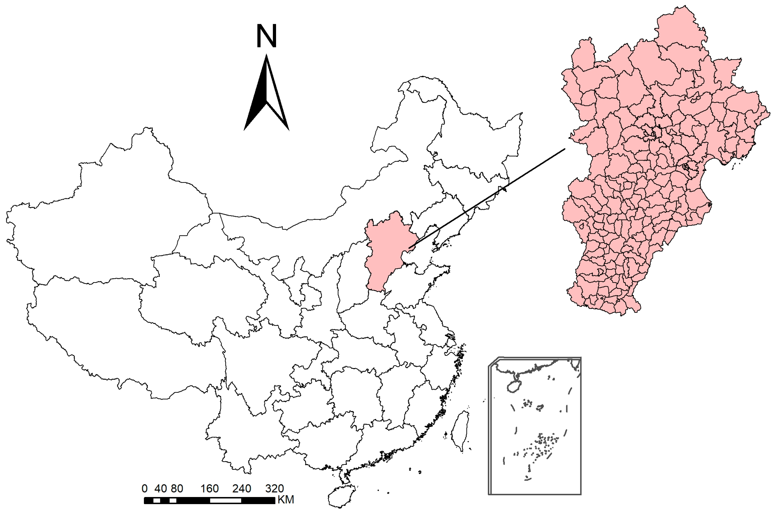
2.1. Study Area

The BTH region is located in the heart of Bohai Rim, bordering Yanshan Mountains in the north, North China Plain in the south, Taihang Mountain in the west, and Bohai Bay in the east. The region includes Beijing City, Tianjin City, and Hebei Province, with a land area of about 220,000 km² and a total population of about 110 million in 2019. In 2001, the development concept of “BTH integration” was put forward (Figure 1). In 2005, Beijing proposed to build itself into a capital economic circle and a world city, to accelerate the development and opening up of the Tianjin Binhai New Area. In addition, Hebei’s strategies to construct a coastal development belt and a green economic circle around the capital were included in “China’s Twelfth Five-Year Plan”. In 2015, the Master Plan for Coordinated Development of BTH was published. In the past 15 years, tremendous changes have taken place in the land-use structure and social economy in the BTH region, which is why the BTH region was selected as the research object to analyze the dynamic value evaluation method of ES from 2000 to 2015.

2.2. Data Sources

The land-use data in this study were from the Data Center of Resources and Environmental Sciences, Chinese Academy of Sciences, and their original data source came from the digital images of Landsat TM with a spatial resolution of 30 m. The interpretation products included six categories and 31 subcategories, with a classification error of less than 2 pixels. The data were in the shp format. The database used for this study was from the years 2000 and 2015. According to the research purpose, land use was divided into 12 categories, namely, paddy field, dry land, forested land, shrub forest, sparse woodland, other woodlands, high-coverage grassland, medium-coverage grassland, low-coverage grassland, water body, desert, and construction land. Social and economic statistics were obtained from Beijing Regional Economic Statistical Yearbook, Tianjin Statistical Yearbook, Hebei Economic Statistical Yearbook, and Hebei Rural Statistical Yearbook in corresponding years (2001 and 2016). All figures were processed in ArcGIS10.2.

3. Materials and Methods

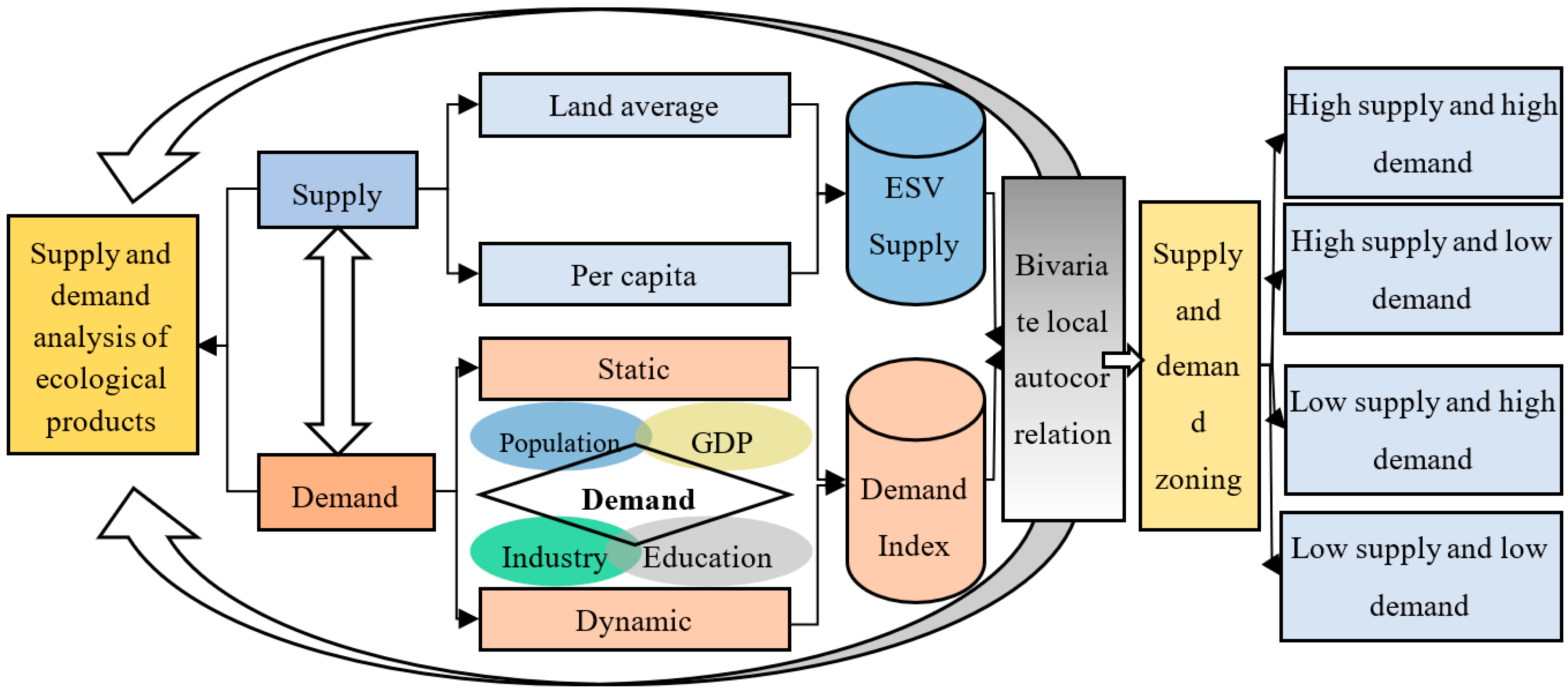
3.1. Evaluation of Supply and Demand of ESV in BTH Region

The concept of supply and demand of ES has not been unified [43]. Yan et al. [44] analyzed the connotation of supply–demand–consumption of ES from different perspectives such as consumption, preference and payment. Ma et al. [45] categorized supply into potential and actual supply, and demand for ecosystem services into realized and total demand. According to Xie et al. [22], the supply function of ES can be divided into 12 categories, namely, air quality, climate regulation, water conservation, soil conservation, waste disposal, biodiversity, food production, raw materials, and recreation and culture. The logical relationship between supply and demand of ES is shown in Figure 2.

3.1.1. Evaluation of NESV

The ES equivalent factors table in China proposed by Xie Gaodi was adopted in this study [22]. According to the national average grain price ratio, the value was revised to that of 2015, and the value level was further corrected from the whole country to the BTH region [46] using the NPP comparison method, so as to determine the NESV of each land-use type (

Table 1. The basic NESV per unit area of each land-use type in the BTH region (CNY/hm²).

Land Use	Air Quality	Climate Regulation	Water Conservation	Soil Conservation	Waste Disposal	Biodiversity	Food Production	Raw Materials	Recreation and Culture	Total Value
Paddy field	1185.632	2110.50	355.77	2596.79	1555.74	420.89	1778.72	118.59	309.70	10,432.33
Dryland	592.816	1055.25	711.41	1731.15	1944.61	841.79	1185.77	118.59	253.93	8435.30
Forested land	4149.98	3464.20	4105.68	5003.81	1680.84	4182.67	128.33	3335.44	1642.27	28,033.87
Shrub forest	3319.984	3117.79	5337.45	4003.02	840.42	3346.17	128.33	3335.44	1313.85	25,014.97
Sparse woodland	2489.988	2274.46	5391.18	2815.88	630.63	2353.89	96.29	2502.67	1078.21	19,670.36
Other woodlands	2074.99	1612.64	5733.86	1863.54	626.00	1947.11	83.70	2173.77	917.46	17,048.54
High-coverage grassland	948.586	1075.14	955.67	2329.56	1564.92	1302.08	358.43	59.67	415.13	9016.25
Medium-coverage grassland	758.842	891.94	1189.30	1932.56	1298.36	1080.24	297.36	49.56	413.56	7945.70
Low-coverage grassland	474.36	549.52	1270.01	1190.66	799.85	665.57	183.26	30.50	338.24	5516.14
Water body	0	549.45	24,344.82	11.88	21,716.91	2974.46	119.48	11.88	5184.27	54,913.14
Desert	0	0.00	37.10	24.78	12.32	421.12	12.32	0.00	140.73	648.37
Construction land	0	0.00	0.00	0.00	0.00	0.00	0.00	0.00	0.00	0.00

). Combined with land-use data in the BTH region, the NESV was calculated using Equation (1).

$$NES{V}_{s,k,t1}=a_{k,t1}\times V{C}_{s,k},$$

(1)

where NESV_s,k,t1 is the NESV of class k on the land use s in year t₁, a_k,t1 is the area of land-use type k at time t₁, and VC_s,k is the unit NESV of class s of land-use type k.

3.1.2. Evaluation of ES Demand

According to the actual situation of the BTH region, population density, per capita GDP, proportion of tertiary industry output value, and adult literacy rate were selected to calculate the ES demand (

Table 2. Index system for ES demand in the BTH region.

Indicator Name	Indicator Meaning	Calculation Method	Positive and Negative	Weight
Population density	The larger the population of the region, the greater the demand for food and ecology	Total population/total area	+	0.30
Per capita GDP	The higher the GDP per capita, the higher the level of economic development, and the higher the demand for environment and culture	GDP/total population	+	0.30
Proportion of output value of tertiary industry	The higher the proportion of output value of tertiary industry, the higher the demand for environment and culture of regional service industry	Tertiary output value/regional output value	+	0.20
Adult literacy rate	The higher the adult literacy rate, the higher the regional education level, and the higher the demand for environment and culture	Literate population/total population	+	0.20

). Specifically, the population density reflects the regional population status, per capita GDP indicates the regional economic development level, proportion of tertiary industry output value demonstrates the regional industrial development status, and adult literacy rate shows the country’s education popularization and regional education level. The extreme value method was used to standardize the evaluation index, and the expert consultation method was used to determine the weight of the index. Taking districts and counties as evaluation units, ES demand in the BTH region in 2015 was evaluated using Equation (2).

$$Dt={{\displaystyle \sum }}_{i=1}^n\left(A_{pi}\times W_i\right),$$

(2)

where Dt is the demand index of evaluation unit, A_pi is the standardized value of index i of unit p, W_i is the weight of the index i, i is the number of the evaluation index, and n is the total number of the evaluation index.

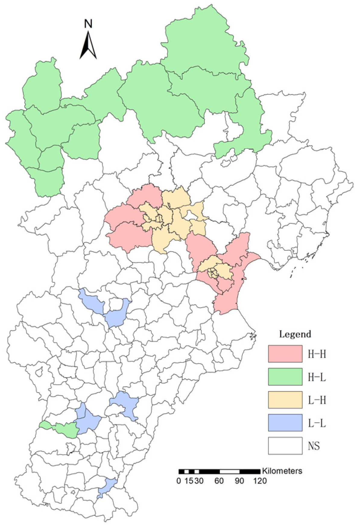
3.1.3. Zoning of Supply and Demand of ESV

The spatial correlation between supply and demand of ESV was determined using the bivariate spatial autocorrelation analysis method, and the supply and demand zones of ESV were divided, which can be expressed as

$$I_{lm}^p=z_l^p{\displaystyle \sum }_{q=1}^n{W}_{pq\ast z_m^q},$$

(3)

where $z_l^{p }$=$\frac{X_l^p-{\overline{X}}_l}{{\sigma }_1}$, $z_m^p$=$\frac{ X_m^q-{\overline{X}}_m}{{\sigma }_m}$, $X_l^p$ is the value of attribute l of the space unit p$, X_m^q$ is the value of the attribute m of the spatial unit q, ${\overline{X}}_l$ and ${\overline{X}}_m$ are the average value of the attributes l and m, and ${\sigma }_1\mathrm{and}{\sigma }_m$ are the variance of the attributes l and m.

3.2. Evaluation of Spatiotemporal Supply–Demand Scarcity of ES

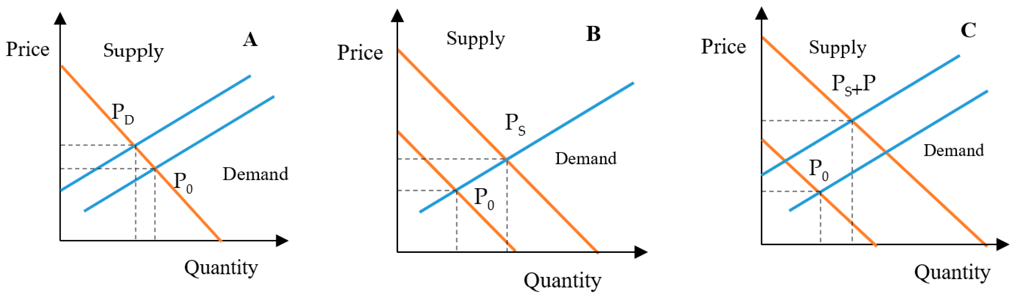
3.2.1. Concept of SESV

Bryan [37] pointed out that, in microeconomics, the basic model of the supply and demand curve mirrors the functional relationship among three variables, namely, price, demand, and supply, from a mathematical perspective. The theoretical basis is that price is an independent variable that determines demand and supply and is positively correlated with supply but negatively correlated with demand. Equilibrium price is produced when supply and demand are balanced. The relationship between supply and demand can predict the quantities of supply and demand caused by price change. The price can also be affected by supply and demand (expressed as value in this study). According to the equilibrium price principle of supply and demand in economics, this paper analyzes the influence mechanism of the temporal change in the supply and demand of ESV on the supply and demand curve of ESV (simplified as a straight line in this paper). Generally, with social and economic development, the regional demand for ES will increase (Figure 3A), while the supply of ES will decrease (Figure 3B). The above two occur simultaneously (Figure 3C), resulting in an increase in the scarcity (value) of ES. Scholars [33] once pointed out that, with the passage of time, the natural environment would become an irreplaceable value-added asset, indicating that the supply and demand of ES will change over time, thus affecting the value of ES and changing the importance (scarcity) of ES.

Combined with the price principle of balance between supply and demand in economics and on the basis of the characteristics of ES in the “hypothetical market”, this paper divides the ESV in the BTH region into private and public types, of which the former is mostly for material products. Their relevant ES can often be attached to the value of agricultural, industrial, or service products, and transformed into commodities that can be directly traded in the market, mostly essential products, such as food and bioenergy. However, public types such as climate regulation and leisure tourism are generally not priced or traded without policy intervention due to market failure (

Table 3. Classification of ES and analysis of elasticity coefficient of supply and demand.

ES	Type of Good	Elasticity
		Demand	Supply
Food production	Private	Inelastic mechanics	Elasticity
Raw material	Private	Inelastic mechanics	Elasticity
Air quality	Public	Elasticity	Inelastic mechanics
Climate regulation	Private	Inelastic mechanics	Elasticity
Water conservation	Private	Inelastic mechanics	Elasticity
Waste disposal	Private	Inelastic mechanics	Elasticity
Soil conservation	Public	Elasticity	Inelastic mechanics
Biodiversity	Public	Elasticity	Inelastic mechanics
Recreation and culture	Public	Elasticity	Inelastic mechanics

).

3.2.2. Evaluation Method of SESV

On the basis of the above analysis, the evaluation method of SESV was put forward [33], which reflects the change of supply and demand in the evaluation of ESV, i.e., with the increase in supply, the demand for SESV increases. It can be specifically calculated as follows:

$$SES{V}_{s,k,t1}=a_{k,t1}\times V{C}_{s,k}\times \left(1+\Delta P_{S,t1}^{Sup}+\Delta P_{S,t1}^{Dem}\right),$$

(4)

where $SES{V}_{s,k,t1}$ is the SESV of class S ES in land-use type k in the year t1$,a_{k,t1}$ is the area of land-use type k at time t1$, V{C}_{s,k}$ is the unit value of ES s of land-use type k, $\Delta P_{S,t1}^{Sup}$ is the change ratio of value caused by supply change, and $\Delta P_{S,t1}^{Dem}$ is the proportion of change in value caused by demand change.

Estimation of ESV change caused by supply change

$$\Delta P_{S,t1}^{Sup}=\Delta Q_{S,t1}^{Sup}\times \Delta p_{S,t1}^{Sup},$$

(5)

$$\Delta Q_{S,t1}^{Sup}=-\frac{{{\displaystyle \sum }}_{k\in K}ES{V}_{s,k,t1}^{Basic}-{{\displaystyle \sum }}_{k\in K}ES{V}_{s,k,t0}^{Basic}}{{{\displaystyle \sum }}_{k\in K}ES{V}_{s,k,t0}^{Native}},$$

(6)

where $\Delta Q_{S,t1}^{Sup}$ is the change ratio of ecosystem service supply, calculated using Equation (6), and $\Delta p_{S,t1}^{Sup}$ is the proportion of changes in the value of ES due to a 100% change in supply, calculated using Equations (10)–(13).

Calculation of ESV change caused by demand change

$$\Delta P_{S,t1}^{Dem}=\Delta Q_{St1}^{Dem}\times \Delta p_{t1}^{Dem},$$

(7)

$$\Delta Q_{t1}^{Dem}=\frac{D_{t1}-D_{t0}}{D_{t0}},$$

(8)

where $\Delta Q_{t1}^{Dem}$ is the change ratio of ecosystem service demand, calculated using Equations (2) and (8), and $p_{t1}^{Dem}$ is the proportion of change in the ESV caused by change in demand, calculated using Equations (10)–(13). After calculating the value of subitems of ES, the total value of regional ES at T time can be calculated as follows:

$$SES{V}_t={\displaystyle \sum }_k{\displaystyle \sum }_{s}SES{V}_{s,k,t}.$$

(9)

According to the sum of elasticity coefficients $\Delta p_{S,t1}^{Sup}\mathrm{and}\Delta p_{S,t1}^{Dem}$ in Equation (4), i.e., assuming that the price of the NESV (the equilibrium point between supply and demand in the initial test year) is 100% at the benchmark time, it is necessary to determine the change in ESV after the simultaneous changes in supply and demand over time. According to Bryan [37], the changes in supply and demand of market-oriented and public welfare ESV, as well as those of price after the simultaneous changes in supply and demand, were deduced.

$$P=1+\frac{2}{\left(e_S+e_D\right)}.$$

(10)

$$P=1+\frac{1+e_D}{\left(e_S+e_D\right)}.$$

(11)

$$P=1+\frac{1}{\left(e_D+e_S\right)}.$$

(12)

$$P=1+\frac{e_D}{\left(e_S+e_D\right)}.$$

(13)

4. Results

4.1. Different Ecological Zoning and Elasticity Coefficient of Supply and Demand

The ES supply was calculated using Equation (1), and the ES demand was evaluated using Equation (2). The spatial correlation between supply and demand of ES was determined through bivariate spatial autocorrelation analysis. Using ESV and the ecosystem service demand index as variables, the local spatial autocorrelation (LISA) aggregation map of the two variables was plotted. The supply and demand of ecosystem services in the BTH region were divided into five categories, namely, high–high (H–H)/low–low (L–L) significant positive spatial correlation, low–high (L–H)/high–low (H–L) significant negative spatial correlation, and no significant spatial correlation (NS). As shown in Figure 4, H–H region was mainly distributed in the suburbs of Beijing and Tianjin, with the H–L region in the northern BTH, L–H region in the main urban areas of Beijing and Tianjin, L–L region mainly distributed sporadically in the southern BTH, and NS region the most widely distributed.

In previous studies, different scenarios were analyzed [37,38]. High, medium, and low conditions were considered in the determination of elasticity coefficient of supply and demand of ESV. The limitation was that the elasticity coefficient of different regions and periods was set as a unified value. Actually, regional difference is an important reason for the imbalance between supply and demand of ES and large value gap between the two. The spatial and temporal differences were considered in the determination of elasticity coefficient in this study. According to the supply and demand pattern of ES, the elasticity coefficient of supply and demand of ESV was determined by regions. A greater demand was correlated with a smaller demand elasticity. Accordingly, the region with a large supply volume had a large supply elasticity, while that with a small supply volume had a small supply elasticity. Therefore, high-supply and high-demand areas (H–H) had high supply elasticity but low demand elasticity, low-supply and high-demand areas (L–H) had both low supply elasticity and low demand elasticity, high-supply and low-demand areas (H–L) had both high supply elasticity and high demand elasticity, and low-supply and low-demand areas (L–L) had both low supply elasticity and low demand elasticity. The elasticity coefficients of different supply and demand zones were identified according to the ecosystem service supply and demand zoning map of the BTH region, as displayed in

Table 4. Determination of elasticity coefficient of different ecological supply and demand zones in the BTH.

Type	Relative Change in SESV	Private Goods		Public Goods
		Supply	Demand	Supply	Demand
High supply and high demand (H–H)	Elasticities	5	0.8	0.1	1.1
	Δ P	0.172	0.172	0.83	0.92
Low supply and high demand (L–H)	Elasticities	2	0.8	0.7	1.1
	Δ P	0.357	0.357	0.55	0.61
High supply and low demand (H–L)	Elasticities	5	0.2	0.1	2.1
	Δ P	0.19	0.19	0.45	0.50
Low supply and low demand (L–L)	Elasticities	2	0.2	0.7	2.1
	Δ P	0.45	0.45	0.357	0.392
Other Areas (NS)	Elasticities	3.5	0.5	0.4	1.6
	Δ P	0.25	0.25	0.5	0.8

Notes: the value of one is unitary elasticity where a 1% change in price results in a 1% change in supply/demand; high elasticity is represented by numbers much greater than one, and high inelasticity is represented by numbers much smaller than one.

.

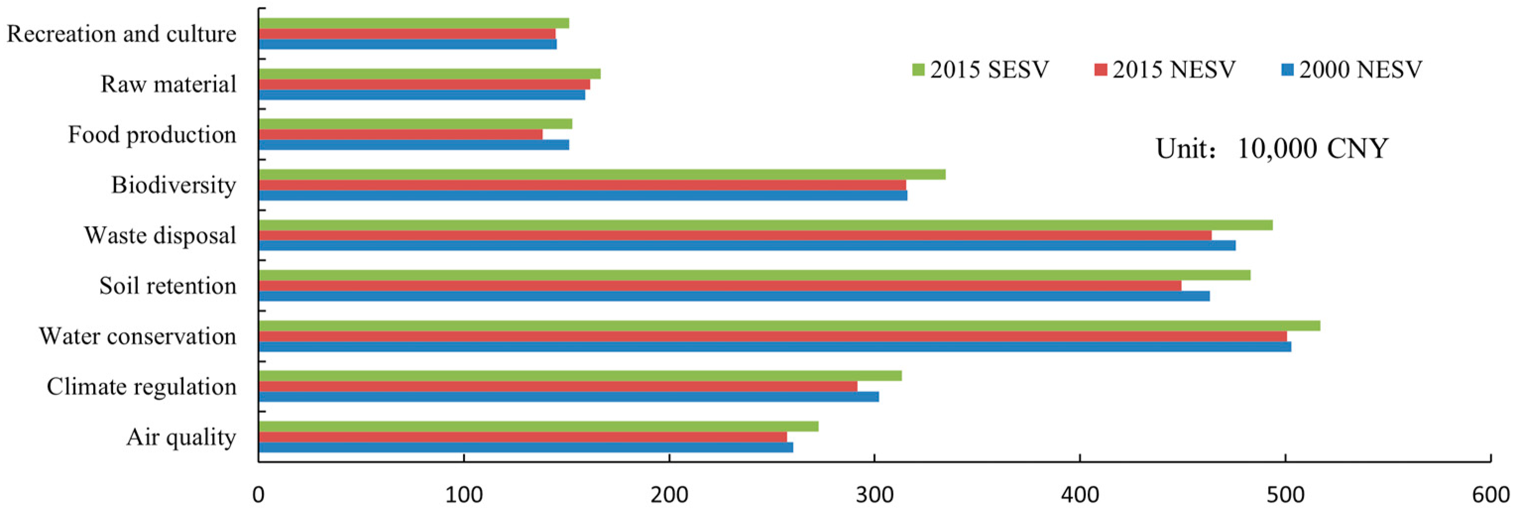
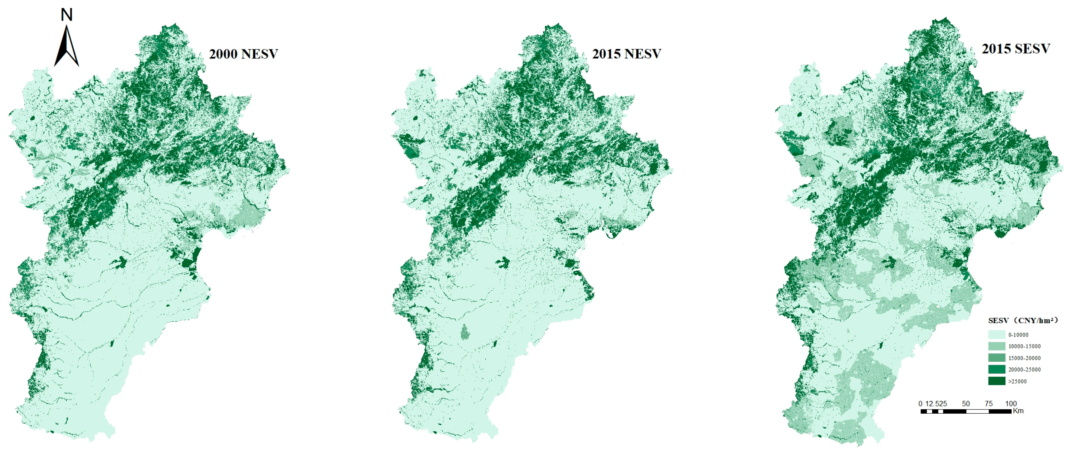
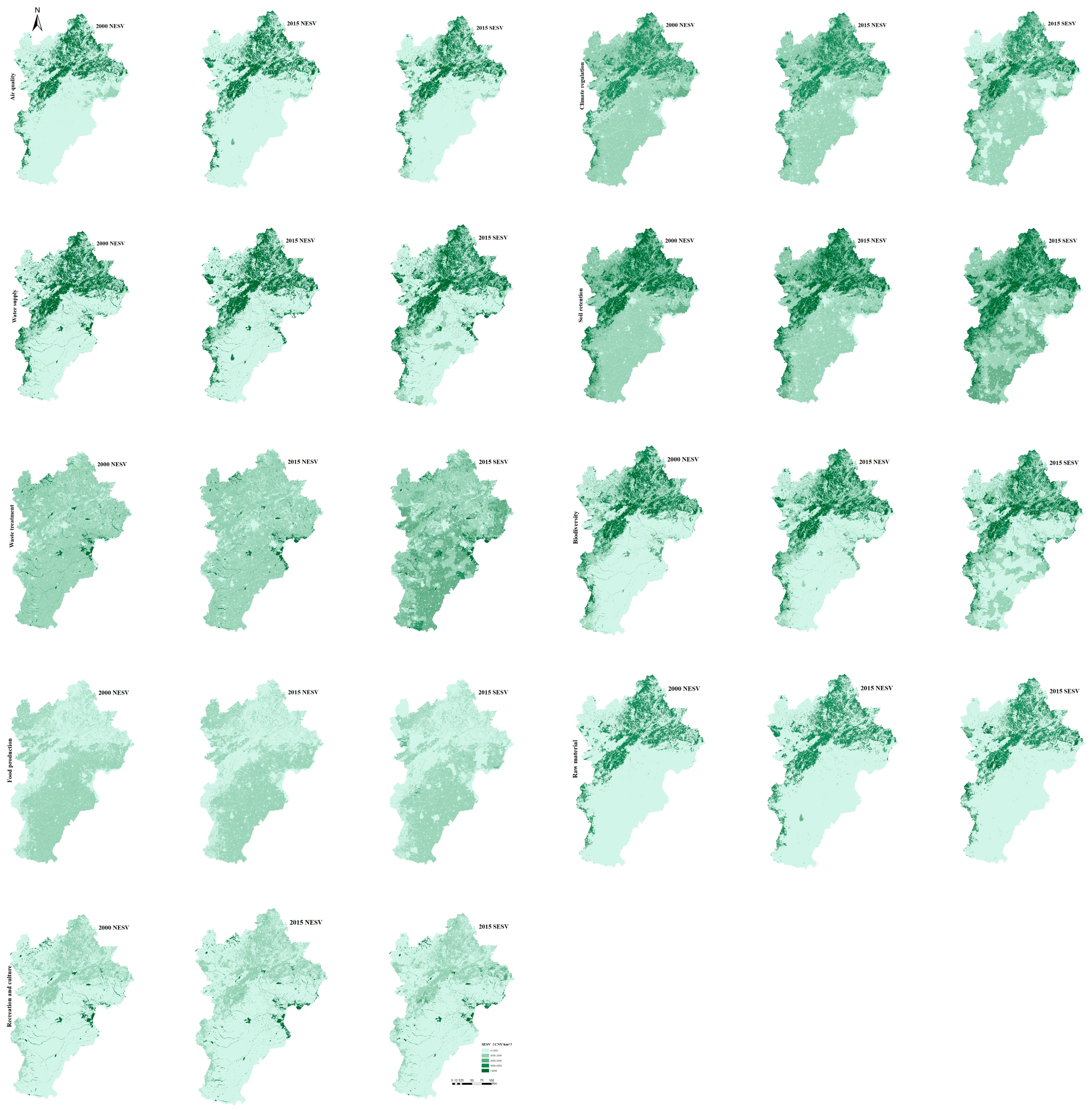
4.2. Changes in NESV and SESV

Figure 5 shows the changing trend of NESV and SESV in the BTH region. As can be seen from the figure, the NESV in the BTH region was 2775.54 billion CNY in 2000, and it decreased to 2722.44 billion CNY in 2015. Considering the changes in supply and demand, the SESV in 2015 was 2884.85 billion CNY. In terms of types, the NESV in 2000 ranked as follows: water conservation > waste disposal > soil conservation > biodiversity > climate regulation > air quality > raw materials > food production > recreation and culture. In 2015, the NESV decreased by 53.07 billion CNY, among which food production had the highest reduction ratio, followed by climate regulation, soil conservation, and waste disposal, with a reduction ratio of more than 2%. The reduction ratios of recreation and culture, biodiversity, and water conservation value were relatively low, while that of raw materials increased to some extent. However, the SESV in 2015 was 109.34 billion CNY higher than the NESV in 2000 and 162.41 billion CNY higher than the NESV in 2015.

Figure 6 shows the distribution of the total ESV in the BTH region. It can be seen from the figure that the NESV in 2000 and 2015 and the SESV in 2015 showed a downward trend from north to south. The northern region was mostly covered with forests, with a relatively high unit price of ESV. In 2015, the total NESV decreased slightly, but with little change in the northern region, while the expanded construction land in the southern plain occupied cultivated land and other land types, resulting in a decrease in the total NESV. However, NESV and SESV in 2015 changed inconsistently. As shown in Figure 6, the SESV in northern China witnessed insignificant change, which was mainly because the supply and demand of ES in the northern region did not change much, while the NESV in the southern region decreased and the demand increased, resulting in an overall rise in the SESV, especially in the surrounding areas of Tianjin, Shijiazhuang, Baoding, etc.

Figure 7 shows the distribution of single ESV in the BTH region. On a whole, the values of air quality, climate regulation, biodiversity, water conservation, soil conservation, and raw material function in the northern region were higher than those in the southern region. The value of waste disposal function was uniformly distributed in the whole region, but the SESV of waste disposal in the southern region in 2015 was significantly higher than that in 2000. The value of food production in the southern region was higher than that in the northern region, the NESV of food production in 2015 was significantly higher than that in 2000, and the SESV of food production in the northern region increased in 2015. The values of recreation and culture were high in two areas, one of which was northern mountainous area, while the other was eastern coastal area. Relatively speaking, little change occurred to NESV and SESV.

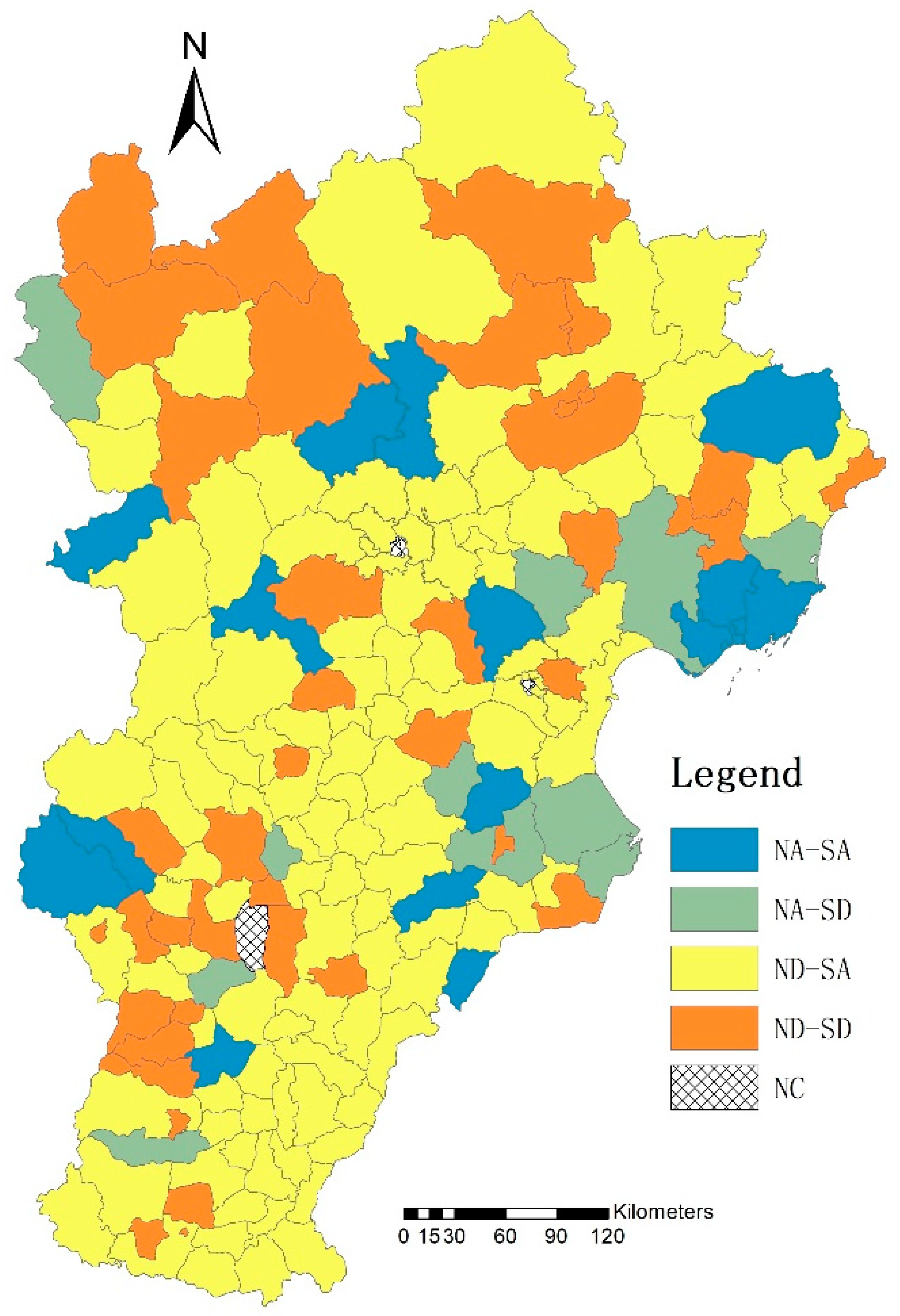
4.3. Ecological Zoning and Land-Use Strategy in the BTH Region

In order to fully understand that changes in regional ecosystem service, it is of great importance to calculate the changes in NESV and SESV in the BTH region while using the country as the evaluation unit. The ecological zoning was divided into five categories, namely, NESV increase–SESV increase (NA–SA), NESV increase–SESV decrease (NA–SD), NESV decrease–SESV increase (ND–SA), NESV decrease–SESV decrease (ND–SD), and no change, as shown in Figure 8. NA–SA areas were scattered in the BTH region, with increased NESV and improved ecological environment. At the same time, the demand and SESV of regional ecosystem increased, which represented benign development. However, it is still important to further optimize the land-use structure, improve supply capacity, and promote the coordinated development of supply and demand. The NA–SD area was mainly distributed in the eastern coastal area, which was in a relatively good state because of improved NESV, increased supply, reduced demand and SESV, and improved regional ecological environment. The ND–SA region was the most widely distributed. The baseline value in the region decreased; however, with economic development and population growth, ecological demand and the SESV increased, especially in the districts and counties around Beijing, Tianjin, Shijiazhuang, and Baoding, where the NESV obviously decreased, while the SESV increased. This represented the core area of economic development in the BTH region. Therefore, it is necessary to attach great importance to land control, limit the conversion from land with high ESV to land with low ESV, and improve the utilization rate of ES. The ND–SD region was mainly distributed in the northern ecological conservation and sporadically in the southern plain. The NESV and SESV were reduced in this region, as were the overall ecological environment quality, regional demand, and SESV. Hence, it is necessary to optimize land-use structure in this region and promote the coordinated development of ecological environment and economy.

5. Discussion

5.1. The Relationship of NESV and SESV

NESV and SESV are different in meaning, in which the former reflects the spatial change in actual physical quantities of regional ecosystems, while the latter reflects the supply and demand capacity of ES, such as reduced supply and increased demand, scarcity, and SESV. The change in SESV is a reflection of the importance of regional ES. The spread of SESV reflects a market failure and demonstrates the growing importance of regional ecosystems and their urgent need to be protected. In previous studies, the change in NESV was often used to reflect that of ESV, and research results reflected the change in the direct quality of regional ES. However, these studies were not comprehensive and objective, as they failed to take into account the change in regional supply and demand and humans’ needs. Through the research of this paper, the relationship between NESV and SESV was clarified, and then the changes in ESV and SESV were explored on the basis of the scarcity effects of spatiotemporal supply–demand influence in the Beijing–Tianjin–Hebei (BTH) region from 2000 to 2015. According to the changes in ecosystem service supply and demand and NESV/SESV in the BTH region, the ecological zones of the BTH region were divided, and differentiated land-use policies were put forward. This research can not only enrich ESV evaluation theories and methods, but also provide a scientific basis for the coordinated development of the BTH region and promote regional ecological civilization construction strategies.

5.2. Application in National Spatial Planning

Land spatial planning can provide a guarantee for ecological civilization construction. Therefore, not only should the status quo of land use be grasped, but the impact of land-use, economic, and social development on regional ES value, especially on public welfare ES value, should also be accurately evaluated and predicted, and their changes should be timely incorporated into the government’s spatial planning and decision making. Due to the importance of different ecological services, NESV and SESV, the government is advised to focus more on reducing urban sprawl and land-use conversion in land spatial planning, which can provide high ESV. Furthermore, it is also of great importance to pay attention to reducing ecosystem service restoration and new land use with high ESV. The dynamic evaluation of ESV, and the analysis of temporal and spatial changes can lay a foundation for scientific and rational decision making of ecological space in land spatial planning. Combined with NESV and SESV of ecosystem services, the important types and regions of ecosystem services supply were determined, and land-use strategies of different supply and demand regions were proposed, which would help ensure the effective supply of ES, identify important ES types and hotspots, and strengthen the supervision of ecological protection red lines. We also suggest to effectively protect ecosystem service resources such as mountains, forests, and water systems, as well as enhance the supply capacity and level of regional ES.

5.3. Application in the Realization of ESV

Ecological compensation and cross-regional transaction of ES are important ways to realize the ESV. In the formulation of ecological compensation standards, the Chinese government has repeatedly proposed to build a market-oriented and diversified ecological protection compensation mechanism. By dynamically evaluating ESV in the BTH region, this study proposed the importance of the ecosystem to regional ecosystem and its changing trend, as well as the basis and standard of regional ecological compensation according to the different supply and demand of the BTH regional ecosystem, so as to improve the efficiency of using ecological compensation funds and embody ecological equity. On the other hand, in the cross-regional transaction of ES, natural economic and social foundations vary among different regions, resulting in great differences in the supply and demand of ES; therefore, it is not appropriate to simply conduct cross-regional transactions at a ratio of 1:1. In the system design of transregional transaction of ESV, the government needs to not only reasonably calculate the NESV of different regions, but determine the value conversion coefficient between ES in different regions. Combined with the results of NESV, the difference in the importance of ES in different supply and demand areas of ES in the BTH region can be evaluated by dynamically evaluating the ESV in the BTH region, which can be used as a reference for the transaction coefficient of ES for different supplies and demands in the BTH region to further promote the cross-regional transaction of ES, facilitate value realization, and improve the transaction efficiency of ES.

6. Conclusions

After 30 years of development, the research on ESV evaluation has gradually shifted from qualitative, static, and single to quantitative and dynamic. The existing evaluation methods of ESV have matured, thus gradually forming relatively perfect evaluation theories and methods. At present, academic circles pay more attention to the evaluation method of the NESV, but there is little research on the dynamic change evaluation system of the ESV as a special product in the market. In recent years, scholars have begun to focus on the relationship between supply and demand of ES, attempting to reflect the relationship between supply and demand in the value assessment of ES.

Aiming at the major national needs of ecological civilization construction and coordinated development of the BTH region, this paper explored the influence mechanism of supply and demand changes in ecosystem value of the BTH region, and then constructed the corresponding method for evaluating ecosystem value. The findings indicate that the NESV in the BTH region decreased without considering the relationship between supply and demand of regional ES, but the SESV increased when the changes in supply and demand were included in the relationship between supply and demand of ES. It should be noted that the increase in SESV is not a reflection of an increase in physical quantity, but an increase in SESV, which represents an increase in the importance of ES, indicating that the ESV in this region requires more protection. By comparing the changing trend of NESV and SESV, we are expected to propose targeted measures against regional land-use structure adjustment and ecological protection. The research results can enrich ESV evaluation theories and methods. It helps to protect important ES in the BTH region and promote the value realization and cross-regional transactions of ES, thus providing a scientific basis for the coordinated development of the BTH region and promoting the strategy of ecological civilization construction, as well as a case study and experience reference for the dynamic evaluation of ESV.

References

1. Costanza, R.; Arge, R.; Groot, R.D.; Farberk, S.; Belt, M. The value of the world’s ecosystem services and natural capital. Nature 1997, 387, 253–260. [Google Scholar] [CrossRef]
2. Lawton, J.H.; Daily, G.C. Nature’s Services. Societal Dependence on Natural Ecosystems. Island Press, Washington, DC. 392 Pp. ISBN 1-55963-475-8 (Hbk), 1 55963 476 6 (Soft Cover). Anim. Conserv. 1998, 1, 75–76. [Google Scholar] [CrossRef]
3. TEEB. The Economics of Ecosystems and Biodiversity for National and International Policy Makers; Welzel+Hardt: Wesseling, Germeny, 2009. [Google Scholar]
4. Sun, S.; Shi, Q. Global Spatio-Temporal Assessment of Changes in Multiple Ecosystem Services under Four IPCC SRES Land-use Scenarios. Earth’s Future 2020, 8, e2020EF001668. [Google Scholar] [CrossRef]
5. Grêt-Regamey, A.; Weibel, B. Global assessment of mountain ecosystem services using earth observation data. Ecosyst. Serv. 2020, 46, 101213. [Google Scholar] [CrossRef]
6. Wang, Z. Study on the Change of Grassland Ecological Service Value and Ecological Compensation in Three-River Headwaters Region, Qinghai, China; China University of Geosciences: Beijing, China, 2019. [Google Scholar]
7. Yu, F.; Yang, W.S.; Ma, G.X. The Latest Development and Prospect of Ecological Value Accounting at Home and Abroad. Environ. Prot. 2020, 48, 18–24. [Google Scholar] [CrossRef]
8. Gundimeda, H.; Sukhdev, P.; Sinha, R.K.; Sanyal, S. Natural Resource Accounting for Indian States—Illustrating the Case of Forest Resources. Ecol. Econ. 2007, 61, 635–649. [Google Scholar] [CrossRef]
9. Sun, M. Research on Land-use Change and the Value of Ecosystem Services in Baiyun Distric; South China Agricultural University: Guangzhou, China, 2016. [Google Scholar]
10. Wu, J.c. Study on Service Value of Island Ecosystem Based on Emergy Analysis---Taking Zhoushan as an Example; Zhejiang Ocean University: Zhoushan, China, 2018. [Google Scholar]
11. Ma, Q.; Liu, K.; Gao, Y.; Ying, L.I.; Fan, Y.; Chao, G.U. Assessment on Social Values of Ecosystem Services in Xi’an Chanba NationalWetland Park based on SolVES Model. Wetl. Sci. 2018, 16, 51–58. [Google Scholar] [CrossRef]
12. Cheng, X.; Damme, S.V.; Li, L.; Uyttenhove, P. Evaluation of cultural ecosystem services: A review of methods. Ecosyst. Serv. 2019, 37, 100925. [Google Scholar] [CrossRef]
13. Rémi, J.; Jérôme, C.; Marti, B.; Stephanie, H. Historical dynamics of ecosystem services and land management policies in Switzerland. Ecol. Indic. 2019, 101, 81–90. [Google Scholar] [CrossRef]
14. Yang, Y.J.; Song, G.; Lu, S. Study on the ecological protection redline (EPR) demarcation process and the ecosystem service value (ESV) of the EPR zone: A case study on the city of Qiqihaer in China. Ecol. Indic. 2020, 109, 105754. [Google Scholar] [CrossRef]
15. Li, D.J.; Yang, L.; Yu, Y.H.; Luo, W.B.; Wang, Z.F. Impact of land use fragmentation on ecosystem service values in an urbanecotourism area: A case study of East Lake ecotourism area, Wuhan. Acta Ecol. Sin. 2019, 39, 1–10. [Google Scholar] [CrossRef]
16. Li, J.M.; Feng, C.C. Ecosystem service values and ecological improvement based on land use change: Acase study of the Inner Mongolia Autonomous Region. Acta Ecol. Sin. 2019, 39, 4741–4750. [Google Scholar] [CrossRef]
17. Ouyang, Z.Y.; Wang, X.K.; Miao, H. A primary study on Chinese terrestrial ecosystem services and their ecological-economic values. Acta Ecol. Sin. 1999, 19, 607–613. [Google Scholar] [CrossRef]
18. Xu, Y.Q.; Zhou, B.T.; Yu, L.; Xu, Y. Temporal-spatial dynamic pattern of forest ecosystem service value affected byclimate change in the future in China. Acta Ecol. Sin. 2018, 38, 1952–1963. [Google Scholar] [CrossRef]
19. Zhao, M.M.; Zhao, H.F.; Li, R.Q.; Zhang, L.Y.; Zhao, F.X.; Liu, L.X.; Shen, R.C.; Xu, M. Assessment on Grassland Ecosystem Services in Qinghai Province during 1998–2012. J. Nat. Resour. 2017, 32, 418–433. [Google Scholar] [CrossRef]
20. Sun, C.; Wang, Y.; Zou, W. The marine ecosystem services values for China based on the emergy analysis method. Ocean Coast. Manag. 2018, 161, 66–73. [Google Scholar] [CrossRef]
21. Xie, G.D.; Zhang, C.X.; Zhang, L.M.; Chen, W.H.; Li, S.M. Improvement of the Evaluation Method for Ecosystem Service Value Based on Per Unit Area. J. Nat. Resour. 2015, 30, 1243–1254. [Google Scholar] [CrossRef]
22. Xie, G.D.; Zhang, Y.L.; Lu, C.X.; Zheng, D.; Cheng, S.K. Study on valuation of rangeland ecosystem services of China. J. Nat. Resour. 2001, 16, 47–53. [Google Scholar] [CrossRef]
23. You, H.M.; Han, J.L.; Pan, D.Z.; Xie, H.C.; Le, T.C.; Ma, J.B.; Huang, S.Z.; Tan, F.L. Dynamic evaluation and driving forces of ecosystem services in Quanzhou bay estuary wetland. Chin. J. Appl. Ecol. 2019, 30, 4286–4292. [Google Scholar] [CrossRef]
24. Xing, L.; Zhu, Y.; Wang, J. Spatial spillover effects of urbanization on ecosystem services value in Chinese cities. Ecol. Indic. 2020, 121, 107028. [Google Scholar] [CrossRef]
25. Tang, X.M.; Chen, B.M.; Lu, Q.B.; Han, F. The ecological location correction of ecosystem service value: A case study of Beijing City. Acta Ecol. Sin. 2010, 30, 3526–3535. [Google Scholar] [CrossRef]
26. You, S.; Kim, M.; Lee, J. Coastal landscape planning for improving the value of ecosystem services in coastal areas: Using system dynamics model. Environ. Pollut. 2018, 242, 2040–2050. [Google Scholar] [CrossRef] [PubMed]
27. Xiong, Y. Agro-Ecosystem Service Value of Sichuan Province: An Assessment. Chin. Agric. Sci. Bull. 2021, 37, 154–160. [Google Scholar]
28. Eigenbrod, F.; Bell, V.A.; Davies, H.N.; Heinemeyer, A.; Gaston, P.R. The impact of projected increases in urbanization on ecosystem services. Biol. Sci. 2011, 278, 3201–3208. [Google Scholar] [CrossRef] [PubMed]
29. Sandhu, H.; Waterhouse, B.; Boyer, S.; Wratten, S. Scarcity of ecosystem services: An experimental manipulation of declining pollination rates and its economic con-sequences for agriculture. PeerJ 2016, 4, E2099. [Google Scholar] [CrossRef]
30. Wang, B.; Tang, H.; Zhang, Q. Exploring Connections among Ecosystem Services Supply, Demand and Human Well-Being in a Mountain-Basin System, China. Int. J. Environ. Res. Public Health 2020, 17, 5309. [Google Scholar] [CrossRef]
31. Ji, Z.; Xu, Y.; Wei, H. Identifying Dynamic Changes in Ecosystem Services Supply and Demand for Urban Sustainability: Insights from a Rapidly Urbanizing City in Central China. Sustainability 2020, 12, 3428. [Google Scholar] [CrossRef]
32. Baumgärtner, S.; Becker, C.; Faber, M. Relative and absolute scarcity of nature. Assessing the roles of economics and ecology for biodiversity conservation. Ecol. Econ. 2006, 59, 487–498. [Google Scholar] [CrossRef]
33. Krutilla, J.V. Conservation reconsidered. Am. Econ. Rev. 1967, 57, 777–786. [Google Scholar]
34. Batabyal, A.A.; Kahn, J.R.; O’Neill, R.V. On the scarcity value of ecosystem services. J. Environ. Econ. Manag. 2003, 46, 334–352. [Google Scholar] [CrossRef]
35. Yahdjian, L.; Sala, O.E.; Havstad, K.M. Rangeland ecosystem services: Shifting focus from supply to reconciling supply and demand. Front. Ecol. Environ. 2015, 13, 44–51. [Google Scholar] [CrossRef]
36. Zank, B.; Bagstad, K.J.; Voigt, B.; Villa, F. Modeling the effects of urban expansion on natural capital stocks and ecosystem service flows: A case study in the Puget Sound, Washington, USA. Landsc. Urban Plan. 2016, 149, 31–42. [Google Scholar] [CrossRef]
37. Bryan, B.A.; Ye, Y.Q.; Zhang, J.E.; Jeffery, D.C. Land-use change impacts on ecosystem services value: Incorporating the scarcity effects of supply and demand dynamics. Ecosyst. Serv. 2018, 32, 144–157. [Google Scholar] [CrossRef]
38. Yu, K.; Cheng, C.X.; Liu, X.H.; Zhang, F.; Li, Z.H.; Lu, S.Q. An ecosystem services value assessment of land-use change in Chengdu: Based on a modification of scarcity factor. Phys. Chem. Earth Parts A/B/C 2019, 110, 157–167. [Google Scholar] [CrossRef]
39. Hu, Q.L.; Qi, Y.Q.; Hu, Y.C.; Zhang, Y.C.; Shen, Y.J. Changes and driving forces of land use/cover and landscape patterns in Beijing-Tianjin-Hebei region. Chin. J. Eco-Agric. 2011, 19, 1182–1189. [Google Scholar] [CrossRef]
40. Xiaomin, G.; Chuanglin, F.; Xufang, M. Coupling and coordination analysis of urbanization and ecosystem service value in Beijing-Tianjin-Hebei urban agglomeration. Ecol. Indic. 2022, 137, 108782. [Google Scholar] [CrossRef]
41. Li, Q.; Li, W.; Wang, S. Assessing heterogeneity of trade-offs/synergies and values among ecosystem services in Beijing-Tianjin-Hebei urban agglomeration. Ecol. Indic. 2022, 140, 109026. [Google Scholar] [CrossRef]
42. Wu, A.; Zhang, J.; Zhao, Y. Simulation and Optimization of Supply and Demand Pattern of Multiobjective Ecosystem Services—A Case Study of the Beijing-Tianjin-Hebei Region. Sustainability 2022, 14, 2658. [Google Scholar] [CrossRef]
43. Burkhard, B.; Kroll, F.; Nedkov, S.; Muller, F. Mapping ecosystem service supply, demand and budgets. Ecol. Indic. 2012, 21, 17–29. [Google Scholar] [CrossRef]
44. Yan, Y.; Zhu, J.Y.; Wu, G.; Zhan, Y.J. Review and prospective applications of demand, supply, and consumption ofecosystem services. Acta Ecol. Sin. 2017, 37, 2489–2496. [Google Scholar] [CrossRef]
45. Ma, L.; Liu, H.; Peng, J.; Wu, J.S. A review of ecosystem services supply and demand. Acta Geogr. Sin. 2017, 72, 1277–1289. [Google Scholar] [CrossRef]
46. Tang, X.M.; Hao, X.Y.; Pan, Y.C.; Gao, Y.B. Ecological Regionalization Based on Ecological Demanding Evaluationin Beijing City. Trans. Chin. Soc. Agric. Mach. 2016, 47, 170–176. [Google Scholar] [CrossRef]
Figure 1. Schematic diagram of the location of BTH region.
Land 11 01545 g001
Figure 2. The relationship between supply and demand of ecosystems.
Land 11 01545 g002
Figure 3. General influence mechanism of the temporal supply and demand of ESV (redrawn from Bryan et al., 2018).
Land 11 01545 g003
Figure 4. Zoning map of ecosystem service supply and demand in the BTH region.
Land 11 01545 g004
Figure 5. Change in NESV and SESV in the BTH region from 2000 to 2015.
Land 11 01545 g005
Figure 6. NESV in 2000 and 2015 and SESV in 2015 of the BTH region.
Land 11 01545 g006
Figure 7. NESV of individual ES in 2000 and 2015 and SESV in 2015 in the BTH region.
Land 11 01545 g007
Figure 8. Ecological zoning in BTH region.
Land 11 01545 g008