
The Impact of Urbanization on Extreme Climate Indices in the Yangtze River Economic Belt, China
by
 , and
, and
Wentao Yang
1,2,* ,
,
Yining Yan
1,2,
Zhibin Lin
2,
Yijiang Zhao
3,
Chaokui Li
1,2,
Xinchang Zhang
4 and
Liang Shan
5,6 1
National-Local Joint Engineering Laboratory of Geospatial Information Technology, Hunan University of Science and Technology, Xiangtan 411100, China
2
Department of Geographical Information Science, Hunan University of Science and Technology, Xiangtan 411100, China
3
Department of Computer Science, Hunan University of Science and Technology, Xiangtan 411100, China
4
Department of Geographical Information Science, Guangzhou University, Guangzhou 510006, China
5
Guangzhou Zengdian Institute of Science and Technology, Guangzhou 511300, China
6
Department of Business Management, Central South University, Changsha 410083, China
*
Author to whom correspondence should be addressed.
Land 2022, 11(9), 1379; https://doi.org/10.3390/land11091379
Submission received: 4 August 2022
/
Revised: 14 August 2022
/
Accepted: 17 August 2022
/
Published: 23 August 2022
(This article belongs to the Special Issue Influence of Urbanization-Related Radical Land Modification on Urban Extreme Climate)
Abstract
:Urbanization has been proven to be a critical factor in modifying local or regional climate characteristics. This research aims to examine the impact of urbanization on extreme climate indices in the Yangtze River Economic Belt (YREB), China, by using meteorological observation data from 2000 to 2019. Three main steps are involved. First, a clustered threshold method based on remote-sensing nighttime light data is used to extract urban built-up areas, and urban and rural meteorological stations can be identified based on the boundary of urban built-up areas. Nonparametric statistical tests, namely, the Mann–Kendall test and Sen’s slope, are then applied to measure the trend characteristics of extreme climate indices. Finally, the urbanization contribution rate is employed to quantify the impact of urbanization on extreme climate indices. The results indicate that urbanization has a more serious impact on extreme temperature indices than on extreme precipitation indices in the YREB. For extreme temperature indices, urbanization generally causes more (less) frequent occurrence of warm (cold) events. The impact of urbanization on different extreme temperature indices has heterogeneous characteristics, including the difference in contamination levels and spatial variation of the impacted cities. For extreme precipitation indices, only a few cities impacted by urbanization are detected, but among these cities, urbanization contributes to increasing the trend of all indices.
1. Introduction
The last decades have witnessed the frequent occurrence of extreme climate events across the world. Although a global warming hiatus (pause or slowdown) is a period of relatively little change in globally averaged surface temperatures, which is mainly manifested by the lower warming rate of the global mean air surface temperature when compared with 1998–2012 [1], the 2000s was the warmest decade on record since 1850, with many regional and global records broken. According to the fifth assessment reports published by the Intergovernmental Panel on Climate Change (IPCC), there is little doubt that extreme climate events with unprecedented frequencies, intensities, and durations will continue to occur in the future [2]. The significant damage to human life and the ecological environment as a result of these extreme climate events has severely hindered sustainable development. Consequently, the 2030 agenda of sustainable development goals released by the United Nations clearly states that all countries should adopt urgent action to address climate change and its impacts [3]. Before measurement and policymaking, it is more significant to understand the association mechanism between extreme climate events and the driving factors.
Urbanization has been proven to be one of the critical driving factors for climate change [4,5]. It changes the radiation, thermal and dynamic characteristics of the underlying surface and alters the land cover in an urban area to be completely distinct from that in surrounding areas, which will result in a horizontal gradient of moisture and energy between the urban area and its surrounding areas and further influence the local or regional climate characteristics [6]. Urban climate change, as a result of urbanization, affects the physical environment more directly than global climate change [7]. According to this fact, a series of studies have focused on analyzing the impact of urbanization on climate change. The main differences in existing research are mainly reflected in the analytical object and study area.
As a common analytical object or a representative phenomenon of urban climate change, the urban heat island (UHI) refers to the warmer temperatures experienced by a city than its surroundings [8]. The UHI magnitude or intensity can be evaluated from two perspectives: one is based on the energy balance differences between urban and rural areas, and the other is by comparing the air temperature between urban and rural areas. The former attempts to compute the types and sizes of heat fluxes generated within an area and then apply the energy balance calculation to account for UHI phenomena [9]. The energy balance can be used for clearly understanding the physical mechanism behind the UHI, but it is difficult to accurately obtain the information about heat fluxes. In contrast, although using the difference in air temperature between urban and rural areas cannot explain the physical mechanism, it is easy to determine the UHI intensity because only air temperature data at different sites need to be obtained. Literature statistics show that this method has been commonly applied to quantify UHIs [10,11].
In addition to the effects on air temperatures, urbanization can also affect extreme precipitation events by changing the formation and development of aerosols, clouds, etc. [12,13]. As demonstrated through an increasing number of studies, these extreme precipitation events are associated with increased urbanization [7,8,9]. Similar to the evaluation of UHI intensity, the commonly used method can also be divided into physical modelling and statistical analysis. Physical modelling aims to apply numerical simulation technology, such as the weather research and forecasting model (WRF), for qualitatively identifying the physical mechanisms of urbanization on precipitation [14,15,16]. However, the requirement of high-resolution data and the uncertainty of the model parameters are obvious limitations. An alternative method is statistical analysis, which is based on the comparison of precipitation between urban and rural stations [17]. Due to the simple computing process, statistical analysis has also been widely used in existing research. Therefore, the statistical method for evaluating the impact of urbanization on extreme climate events was used in this study.
Nevertheless, whether the statistical method is used to analyze the effects of urbanization on UHI intensity or extreme precipitation, how to select urban and rural stations poses significant challenges because many relevant local-scale aspects need to be considered [18]. According to the difference in the main data source, existing methods for classifying stations can be roughly divided into two categories: one is mainly based on climate data, and the other is based on auxiliary data (population data, land use and land cover (LULC)). The former, such as empirical orthogonal function (EOF) decomposition and interpolation isotherms, attempt to address the classification issue by highlighting different thermal or climate characteristics in urban-rural pairs [19,20]. These methods can exhibit an obvious advantage when considering the boundary of the urbanization effect, but the sparse distribution of meteorological stations in most urban areas cannot effectively support these mathematical methods.
In contrast, these methods based on auxiliary data first extract urban built-up areas, and meteorological stations located in (outside) the urban built-up areas are then identified as urban stations (rural stations). Obviously, the crucial issue is to accurately obtain urban built-up areas. The spatial distribution of population density is one of the main sources used to extract urban built-up areas. Specifically, a threshold for the population needs to be set in advance, and an area with a higher value than the threshold is identified as a built-up area [21]. Nevertheless, it is difficult to determine the threshold because the population change with urban areas and to obtain accurate population data at a fine scale need to be further discussed. Remote sensing nighttime light data are useful for extracting large-scale built-up urban areas and have also been used to identify urban and rural stations [22]. Compared with other auxiliary data, namely, population data and LULC, remote sensing nighttime light data can be directly collected by sensors and effectively reveal the area of human activities, which has attracted increasing attention in extracting urban built-up areas. However, empirical threshold-based methods were selected to extract urban built-up areas in previous studies on meteorological station classification [23]. They may overestimate the built-up areas in urban regions due to the ‘blooming’ effect of nighttime lights and over small patches in developing towns because of the relatively low value of nighttime lights. Consequently, an inaccurate result of urban built-up areas will result in error in station classification and further lead to an unreliable result of the impact of urbanization on UHIs or extreme precipitation. In this research, a clustered threshold strategy was used to extract urban built-up areas by remote sensing nighttime light data, which can avoid the above issues resulting from the empirical threshold-based method.
In addition, due to the spatial heterogeneity of urban characteristics, such as land cover, impermeable layers, and industrial structures, the impact of urbanization on UHIs or extreme climate indices may vary with the study area or scale [24,25,26,27]. The Yangtze River Economic Belt (YREB), China, was selected as the study area. The YREB was positioned as a coordinated development belt for western, central, and eastern parts of China, a pioneering and demonstration belt for ecological and green civilization, and an inland river economic belt with a global influence [28]. The outline of the Yangtze River Economic Belt Development Plan, released in March 2016, further emphasized a development pattern for the area with concentrations on ecological and green civilization [29]. Undoubtedly, this national strategy would provide an unprecedented opportunity for in-depth development of the cities in the YREB. However, in recent decades, because of urbanization processes, climate conditions in the YREB have obviously changed [30]. The disastrous floods and extreme temperature events associated with climate change occurred frequently and resulted in considerable economic loss and human lives in the YREB [31]. Therefore, it is of great significance to understand the impact of urbanization on extreme climate events in the YREB.
The remaining paper is organized as follows. Section 2.1 introduces the study area and datasets. Section 2.2 introduces the method for identifying the impact of urbanization on extreme climate indices. The experimental results are described in Section 3. The conclusion and discussion are presented in Section 4 and Section 5, respectively.
2. Materials and Methods
2.1. Study Area and Datasets
As the longest river in China and the third-longest river in the world, the mainstream Yangtze River flows through two municipalities (Chongqing and Shanghai) and nine provinces (Anhui, Guizhou, Hubei, Hunan, Jiangsu, Jiangxi, Sichuan, Yunan, and Zhejiang). The area covering these 11 provincial-level regions is called the YREB, which occupies 2.05 million square kilometers, accounting for approximately 21.3% of China’s land area. In 2017, the total population and GDP in the area were approximately 595 million and 37,100 billion yuan, which correspond to 42.8% and 44.9% of the country’s total, respectively [29]. The spatial distribution of the 11 provincial-level regions is shown in Figure 1, and each region is marked with a unique colour.
The time series of daily maximum/minimum temperature and daily precipitation for 20 years (2000–2019) were obtained from the China Meteorological Data Service Centre (http://data.cma.cn/en accessed on May 12, 2022). After the meteorological stations with a large amount of missing data were removed (the proportion of missing data at some sites was higher than 30%), there were 252 meteorological stations in the YREB, accounting for 96% of the total number of all stations. Based on meteorological data at 252 stations, the software package RClimDex (http://etccdi.pacificclimate.org/software.shtml accessed on May 12, 2022) was applied to compute 27 extreme climate indices, including 16 extreme temperature indices and 11 extreme precipitation indices [32]. A brief introduction of these extreme climate indices is shown in Table 1. In addition, the vector map in the YREB [33] was also collected as auxiliary data for visualization and verification analysis. To distinguish urban and rural meteorological stations, remote-sensing nighttime light data [34] and built-up area data [35] were collected.
Admittedly, because of changes in observation stations, instruments, schedules, and habits, inhomogeneous data or discontinuous points can be created [36]. The inhomogeneous data may cause deviations in estimating climate trends, resulting in inaccurate analyses for regional climate detection [37]. It is critical to perform data homogenization so that the homogenous time series of climate variables contain only climate variation and regional trend information. In this study, there are nine stations whose locations have changed at least once. We deleted these climate data from these stations instead of adjusting them. Compared with the number of all stations, the number of stations with location changes is less, and detecting these few stations may not have much impact on the analysis results.
2.2. Methods
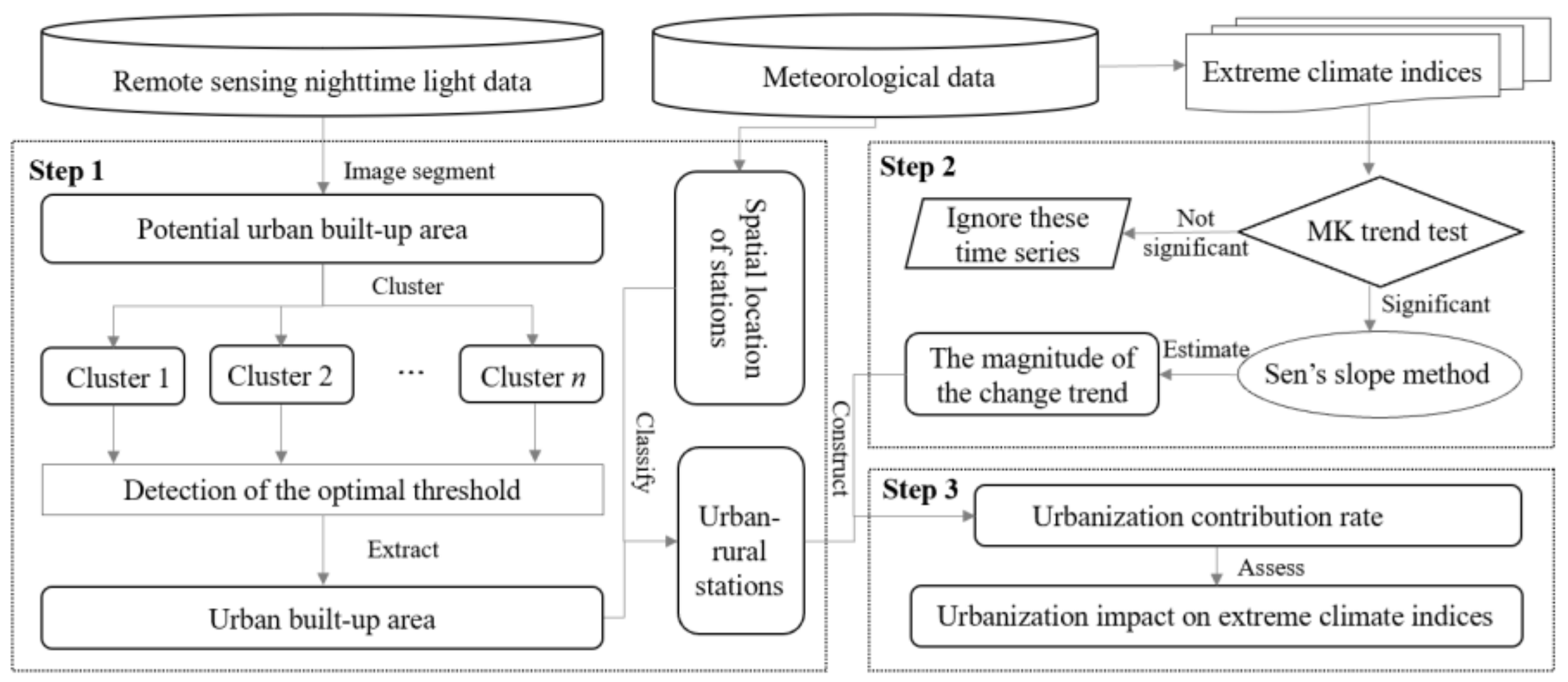
As mentioned in the first section, the statistical method for evaluating the impact of urbanization on extreme climate events was used in this study [38,39,40], but how to accurately identify urban and rural stations is crucial for the statistical method to evaluate urbanization on extreme climate indices. This research aims to apply a remote sensing method of selecting urban and rural stations for evaluating urbanization on extreme climate indices in the Yangtze River Economic Belt, China. The framework of this research is shown in Figure 2. The main process can be divided into three steps. First, a clustered threshold strategy based on remote-sensing nighttime light data is used to extract urban built-up areas [41], and urban and rural stations can be identified by the boundary of urban built-up areas [42,43,44], as described in Section 2.2.1. Second, the Mann–Kendall test is applied to determine the significant trends among the time series of extreme climate indices [45]. For the time series of an index at one station, if a significant increasing or decreasing trend is confirmed, then Sen’s slope method is used to estimate the magnitude of the change trends of extreme climate indices [25]. Otherwise, the time series at the station is ignored in the subsequent analysis. The detailed introduction is described in Section 2.2.2. Third, based on the change trend of extreme climate indices at urban and rural stations, the urbanization contribution rate is applied to assess the impact of urbanization on extreme climate indices, as described in Section 2.2.3.
2.2.1. Classifying Meteorological Stations Using a Remote Sensing Method
The remote sensing method was used in this research to classify meteorological stations into urban and rural stations. This method first extracts urban built-up areas by using remote sensing nighttime light data, and according to the topological relation between urban built-up areas and meteorological stations, the meteorological stations will be classified into urban and rural stations. Specifically, the meteorological stations located in the urban built-up areas are defined as urban stations, and those located outside the urban built-up areas are defined as rural stations. Obvious differences in nighttime light intensity exist among urban areas with different urbanization levels because of varied urban development stages and energy consumption patterns. Therefore, the threshold for extracting urban built-up areas from nighttime light should change with the level of nighttime light intensity. It is reasonable to apply a clustered threshold strategy to handle this task.
The clustered threshold strategy mainly includes three steps. First, an image segmentation algorithm is used to obtain the potential urban built-up areas, which is defined as a set of areas composed of spatially continuous lighted pixels in the single-band nighttime light. A series of image segmentation algorithms have been proposed for object-based classification in remote sensing. Considering that the marker-controlled watershed segmentation algorithm based on greyscale morphology is suitable for single-band remote sensing nighttime light images, this algorithm is used to obtain the potential urban built-up areas. The detailed process can be found in the relevant literature [41].
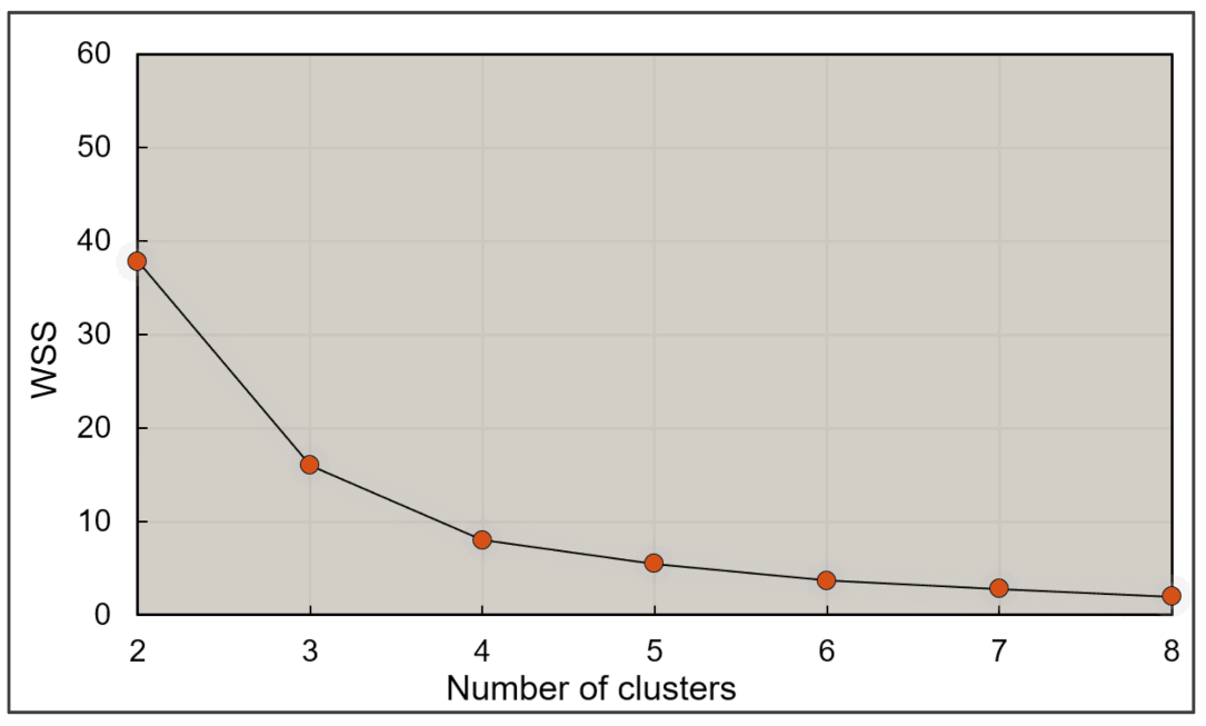
Then, a clustering algorithm is applied to divide the potential urban built-up areas into several groups with similar nighttime light intensities. As only the total digital number of nighttime lights needs to be considered in the clustering process, the classical k-means algorithm is used to divide the potential urban built-up areas [46]. The elbow method was used to determine the optimal cluster number k [47]. It considers the variation characteristics of the sum of squared deviations from the means in each cluster, the within sum of squares (WSS), which is defined as
where is the number of objects belonging to the jth cluster; and are the total DN values of the ith objects of the jth cluster; and is the mean DN value of all the objects of the jth cluster. At some value for k, the WSS drops dramatically, and after that it reaches a plateau when the value of k continues to increase. This point, when this decrease in WSS dispersion slows down, is called the “elbow” [48]. In this situation, the optimal cluster k can be identified, and the clustering result is used to determine different thresholds for extracting urban built-up areas.
Finally, for each cluster, the optimal threshold to classify the urban and rural areas is detected by comparing the areas of the statistical data and urban built-up areas with different thresholds. That is, the statistical data through an official survey always accurately record the total area of each urban built-up area. The different results of the built-up areas can be obtained based on a set of thresholds. The total area of the built-up area can be directly based on the number of pixels whose DN values are larger than the threshold. The optimal threshold corresponds to the built-up area closest to the statistical data. Specifically, assume that the set of thresholds is t= {t1, …, tn} (i = 1, …, n), and for each threshold, the total area of the built-up areas A(ti) (i = 1, …, n) can be obtained by counting the number of pixels whose DN values are larger than ti. The optimal threshold for a cluster can be computed as
where is the total area of each urban built-up area from an official survey.
2.2.2. Identifying the Change Trends of Extreme Indices
In this study, the nonparametric Mann–Kendall (MK) test is used to detect the significant trends among the time series of extreme climate indices. A positive (negative) value of the MK statistic indicates an increasing (decreasing) trend in the data. For a sample size >10, a normal approximation to the Mann–Kendall statistics Z can be applied to test significance. If Z is greater than , where α is the significance level (0.10 in the study), it is considered a significant trend [49].
The Sen’s slope method was selected to estimate the magnitude of the change trend of extreme climate indices. As a nonparametric method, Sen’s slope assumes a linear trend in the time series and then applies a linear model to calculate the slope of the trend [50]. A positive value of the estimator corresponds to an increasing trend, and a negative value indicates a decreasing trend in the time series. As the slope estimator is calculated through the median statistic, Sen’s slope is robust to outliers and missing data.
2.2.3. Assessing the Impact of Urbanization on Extreme Climate Indices
The impact of urbanization on extreme climate indices can be reflected by the linear trend changes in extreme climate indices at urban stations resulting from urbanization [51]. The impact value Δβ can be defined as:
where and indicates the change trend of extreme climate indices at urban and rural stations, respectively. A positive value of the impact value corresponds to an increasing trend of urbanization on extreme climate indices, and a negative value indicates a decreasing trend of urbanization on extreme climate indices. Furthermore, the urbanization contribution rate is expressed as:
where if is equal to 0, it means that urbanization has no contribution to the extreme index extreme at urban stations, and if is equal to 100%, it means that the change trend of extreme climate indices at urban stations is completely caused by urbanization. Notably, because some unknown local factors may exist, the values of the urbanization contribution rate may be greater than 100%, and in this case, the urbanization contribution rate is also regarded as 100% [52].
3. Results
3.1. Classification of Meteorological Stations
As introduced in Section 2.2.1, the watershed segmentation algorithm was first used to obtain the potential urban clusters. The spatial distribution of potential urban built-up areas is shown in Figure 3, and the orange area indicates the potential urban built-up area. The nighttime light intensity of potential urban built-up areas was then aggregated into prefecture-level cities based on the administrative boundary. Furthermore, the number of clusters defined using the k-means cluster algorithm over the nighttime light intensity was tested for k = 2, …, 8. The estimates of WSS for different k are visualized in Figure 4. The number of clusters was set to 4 since the WSS drops dramatically when k is from 3 to 4 and reaches a plateau when k is from 4 to 5. The cluster result is presented in Figure 5, and these four clusters are displayed in different colors. From Cluster 1 to 4, the nighttime light intensity of prefecture-level cities gradually increases, but the number of these cities gradually decrease.
For each cluster, different results of extracting the built-up areas can be computed based on a set of thresholds. In Figure 6, the horizontal axis indicates the DN threshold, and the vertical axis represents the absolute value of the difference between the built-up area from the remote sensing data and the statistical data. Based on Equation (2), the optimal threshold corresponds to the lowest value of the cures in Figure 6. Therefore, the optimal thresholds for Cluster 1 to 4 are 2, 18, 21, and 23, respectively. According to the optimal threshold of each cluster, the final urban built-up areas can be identified. Furthermore, urban and rural stations can be separated based on the boundary of these built-up areas. The total number of urban and rural stations are 203 and 41, respectively. The spatial distribution of urban and rural stations is shown in Figure 7, and the orange squares and blue circles indicate rural and urban stations, respectively.
Notably, a potential assumption in Equation (3) is that the urban and rural stations are usually distributed in adjacent locations. Due to the significant difference in the number of stations between urban and rural areas, the nearest rural stations of some urban stations may be far away from them and have different climate characteristics that not only result from the urbanization. In that case, the urban stations should be ignored because of the lack of nearby rural stations as a reference. Consequently, to filter out these cities and retain the prefecture-level cities with higher urbanization levels, we built a 110 km buffer zone centered on each rural station, and these urban stations within a buffer are reserved. Here, a buffer radius that is too large violates the principle of proximity between urban and suburban stations, which may lead to extreme climate impacts not completely caused by urbanization. Too small a buffer radius may lead to many cities not referring to rural stations. Considering the above conditions, the buffer radius was selected as 110 km. In this situation, the radius was not too large, and more rural stations could be matched to urban stations. Finally, 99 urban stations (or cities) and 38 rural stations were determined, which are shown in Figure 8.
3.2. The impact of Urbanization on Extreme Temperature Indices
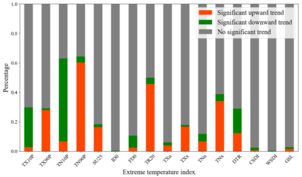
For each extreme temperature indices, the MK test and Sen’s slope method were first used to detect the significant trends among time series at both urban and rural stations. The statistical results are listed in Figure 9. The horizontal axis represents extreme temperature indices, and the vertical axis indicates the proportion of cities with different trend types in the number of all cities. Overall, these indices, including TN90P, TR20, TNx, and TX90P, exhibit significant upward trends, and TX10P and TN10P show significant downwards trends at most stations. There are no significant or dominant trends in the remaining indices. The indices with significant upward trends mainly consist of warm indices (TN90P, TR20, and TX90P). Meanwhile, all the indices with significant downwards trends (TN10P, and TX10P) are cold indices.
Furthermore, based on Equations (3) and (4), the urbanization contribution rates on TN90P, TR20, TNx, TX90P, TN10P, and TX10P can be obtained. The spatial distribution and urbanization contribution rates of the impacted cities are shown in Figure 10. Only cities in which extreme temperature indices had a significant impact caused by urbanization are labelled in Figure 10. The red and green triangles represent the impact of urbanization with a dominant upwards and downwards trend, respectively, and the size of triangles represents urbanization contribution rates, which was divided into four intervals, namely, [0%, 25%), [25%, 50%), [50%, 75%), and [75%, 100%]. Among all 99 cities, the total number of cities in which TN90P, TR20, TNx, TX90P, TN10P, and TX10P were impacted by urbanization was 36, 24, 9, 11, 20, and 7, respectively. Among these indices affected by urbanization with a dominant upwards trend, TN90P was the most severely affected by urbanization, followed by TR20. Both TNx and TX90P are similarly affected by urbanization, but only a very small number of cities were detected. It can also be found that the spatial distribution of these cities is inconsistent. Cities of which TN90P, shown in Figure 10a, was impacted by urbanization covered most areas of the YERB. However, most of them are distributed in the middle reaches, including Chonqing, Guizhou, Hubei, and Hunan Provinces, where the urbanization contribution rates are mainly located in the range of 25% to 75%. Overall, other cities located upstream and downstream have low contribution rates. In Figure 10b, cities of which TR20 was impacted by urbanization are also mainly distributed in the middle reaches with a high variance of urbanization contribution rates (the range is from 0% to 75%). The downstream cities with high values of urbanization contribution rates are in Anhui Province. For the cities in which TNx and TX90P were impacted by urbanization, as shown in Figure 10c,d, there was no spatial aggregation pattern.
In the indices impacted by urbanization with a dominant downwards trend, TN10P is more seriously impacted by urbanization than TX10P. As shown in Figure 10e, cities corresponding to TN10P are mainly distributed in the middle reaches of the YERB, including Chongqing and Hubei provinces, and many values of urbanization contribution rates are greater than 50%. Although TX10P was not severely impacted by urbanization, as shown in Figure 10f, the spatial distribution of the impacted cities exhibits an agglomeration pattern, and most of the cities are located in Sichuan Province.
3.3. The Impact of Urbanization on Extreme Precipitation Indices
Similarly, the nonparametric statistical test was applied to identify different types of trends among the time series of extreme precipitation indices at both urban and rural stations. The statistical results are shown in Figure 11. For all extreme precipitation indices, the number of cities with no significant trend is the largest. In the cities in which the index has a significant trend, there are more cities with an upwards trend than those with a downwards trend. Only cities of which Prcptot was impacted by urbanization are spatially clustered and mainly located downstream of YERB, as shown in Figure 12.
4. Discussion
Understanding the impact of urbanization on extreme climate events is a crucial topic in climate change. This research used the statistical comparison of extreme climate between urban and rural stations to measure the impact of urbanization on extreme climate events. Compared with physical modelling, statistical analysis exhibits obvious advantages and limitations. It can be directly used to measure the impact based only on climate data from different stations, but the method cannot describe the physical mechanism behind these climate processes. Among the statistical methods, an important process was how to classify meteorological stations into urban and rural stations, which was further converted to the issue of the identification of urban built-up areas. Therefore, a clustered threshold strategy based on nighttime light data was then presented to handle this issue. Compared with other methods, such as empirical orthogonal function decomposition and interpolation isotherms, the remote sensing method only involves nighttime light data, which are easily accessible, and the principle for meteorological station classification is also easy to understand.
The YREB with rapid urbanization development was selected as the study area. Previous studies on the extreme climate of the YREB [53] mainly focused on the characteristics of extreme temperatures [45] and extreme precipitation [54] and rarely explored the impact of urbanization on the extreme climate of the YREB [55]. In this research, it was found that the number of meteorological stations with significant trends for extreme temperature indices was higher than that for extreme precipitation indices. This conclusion was also demonstrated in related studies. For example, Cheng et al. found that the number of extreme temperature indices with significant changes in the Yangtze River Basin from 1958 to 2017 was 2.8 times that of the extreme precipitation index [55]. Among these extreme temperature indices, warm indices, including TN90P, TR20, and TX90P, always exhibit an upwards trend, and most of the cold indices, such as TN10P and TX10, show a decreasing trend in the study area, which is also consistent with the results in other regions or local regions in the YREB. For example, Zhao et al. found that the warm indices showed upwards trends in the Beijing-Tianjin-Hebei regions during the period 1980-2015, while the cold indices tended to decrease [25]. Shi et al. found that the main cold index of the extreme temperature index in the Yangtze River Basin showed a downwards trend from 1970 to 2014, and the main warm index of the extreme temperature index showed an upwards trend [45].
The urbanization contribution rates were used to quantitatively measure the impact of urbanization on extreme climate indices. The impact of urbanization on extreme temperature indices has obviously heterogeneous characteristics, which is mainly reflected in the following two aspects. One is that urbanization has distinct levels of impact on different extreme temperature indices, and TN90P, TR20, and TN10P were seriously affected by urbanization. The other is that the impact of urbanization on different indices has spatial variability; that is, for different extreme temperature indices, the spatial distribution of the impacted cities is inconsistent. For example, cities in which TN90P, TR20, and TN10P were impacted by urbanization are mainly distributed in the middle reaches, and most of the cities in which TX10P exhibits a downwards trend are located in Sichuan Province. This similar conclusion was also demonstrated in related studies. For example, Qiu et al. found that extreme temperature indices (TNn, TXx) in China increased significantly from 1960 to 2016 with varying degrees in different seasons and different regions [52]. Lin et al. found that in 20 urban agglomerations in China from 1971 to 2014, for both extreme temperature and precipitation indices, urban and rural areas exhibit remarkably distinct changes and demonstrate a significant urbanization effect, which also varies across different climate backgrounds [26].
The impact of urbanization on extreme precipitation indices was lower than that on extreme temperature indices, which indicates that extreme precipitation indices were not susceptible to urbanization in the YREB. The impacts on extreme precipitation indices display stronger regional discrepancies than those on temperature extremes [26]. In previous studies, there was no consistent conclusion on the impact of urbanization on extreme precipitation indices. Some researchers found that urbanization caused great precipitation and heavy precipitation frequency [56], and one potential reason is that because of the effect of urban heat islands, local thermodynamics and unstable atmospheres may result in stronger precipitation in urban areas [57]. Other researchers demonstrated that the increase in aerosols and the associated cloud microphysical process could cause the reduction in precipitation in the urbanization process [58], and a downwards trend of extreme precipitation indices might be exhibited in some cities [59]. The results in this research demonstrated that the extreme precipitation indices of only a few cities exhibited a significant trend, so urbanization did not absolutely affect the 9 extreme precipitation frequencies.
In addition, we also found that the cities of which Prcptot was significantly impacted by urbanization were concentrated in the Yangtze River Delta, especially in Zhejiang Province. Meanwhile, Prcptot shows a downwards trend in these areas. However, in the study of Yuan et al., the change trend of Prcptot in the Yangtze River Basin from 1961 to 2020 was not significant [50], and Prcptot was not proven to be impacted by urbanization. This research found that TX90P had the most significant growth trend of 5.7 days/10 years only in Yunnan Province. However, Shi et al. found that from 1970 to 2014, warm days (TX90P) in the Yangtze River Basin obviously increased, with a trend of 4.73 days/10 years [45].
This research only focuses on quantifying the impact of urbanization of cities on different extreme climate indices in the YREB and was not conducive to a deep discussion regarding the potential association relationship, namely, how to explain the heterogeneous characteristics of the impact of urbanization on extreme climate indices. The above content needs to be discussed in future research.
5. Conclusions
In this research, the impact of urbanization on extreme temperature and precipitation indices in the YREB was examined by comparing the trend characteristics of urban and rural stations. The specific process mainly includes three steps: a clustered threshold method based on remote-sensing nighttime light data is first applied to extract urban built-up areas, and urban and rural meteorological stations can be identified based on the boundary of urban built-up areas. The total numbers of urban and rural stations were 203 and 41, respectively, and 99 urban stations with corresponding rural stations were finally selected. The nonparametric statistical method is then applied to measure the trend characteristics of extreme temperature and precipitation indices. The warm indices (TN90P, TR20, and TX90P) show significant upwards trends, and all the indices with significant downwards trends (TN10P and TX10P) were cold indices. Except for a few cities in which extreme precipitation indices show an upwards trend, those indices did not exhibit a significant trend in most urban areas. Based on the change trend of extreme climate indices at urban and rural stations, the urbanization contribution rate is applied to assess the impact of urbanization on extreme climate indices. Overall, urbanization has a more significant impact on extreme temperature indices than on extreme precipitation indices. Urbanization leads to a more (less) frequent occurrence of warm (cold) events. The impact of urbanization on different extreme temperature indices has heterogeneous characteristics, which are reflected in the difference in contribution levels and spatial variation of the impacted cities. The extreme precipitation indices of only a few cities exhibited a significant trend, so urbanization did not absolutely affect the frequency of the nine extreme precipitation events.
Author Contributions
Conceptualization, Z.L. and W.Y.; methodology, W.Y., Y.Y, and Y.Z.; software, Y.Z. and L.S.; validation, Y.Y., Z.L., and L.S.; formal analysis, C.L. and X.Z.; investigation, Z.L.; resources, Y.Z.; data curation, Z.L.; writing—original draft preparation, W.Y.; writing—review and editing, W.Y., Y.Y.; visualization, Y.Y., Z.L. and Y.Z.; supervision, C.L. and X.Z.; project administration, W.Y. and X.Z.; funding acquisition, W.Y. All authors have read and agreed to the published version of the manuscript.
Funding
This research was funded by the Foundation for Innovative Research Groups of the Natural Science Foundation of Hunan Province, grant number 2020JJ1003, Natural Science Foundation of Hunan, China, grant number 2021JJ30245 and 2022JJ60015, the Philosophy and Social Science Foundation of Hunan Province, China, grant number 18YBQ050, and Open Research Fund Program of LIESMARS, grant number 19I04.
Institutional Review Board Statement
Not applicable.
Informed Consent Statement
Not applicable.
Data Availability Statement
Not applicable.
Acknowledgments
We express our sincere appreciation to the anonymous reviewer for constructive comments.
Conflicts of Interest
The authors declare no conflict of interest. The funders had no role in the design of the study; in the collection, analyses, or interpretation of data; in the writing of the manuscript, or in the decision to publish the results.
References
- Chatzopoulos, T.; Perez Dominguez, I.; Zampieri, M.; Toreti, A. Climate extremes and agricultural commodity markets: A global economic analysis of regionally simulated events. Weather Clim. Extrem. 2020, 27, 100193. [Google Scholar] [CrossRef]
- Liao, H.; Chang, W. Integrated assessment of air quality and climate change for policy-making: Highlights of IPCC AR5 and research challenges. Natl. Sci. Rev. 2014, 1, 176–179. [Google Scholar] [CrossRef]
- United Nations. Transforming Our World: The 2030 Agenda for Sustainable Development. Available online: https://sustainabledevelopment.un.org/post2015/transformingourworld/publication (accessed on 12 May 2022).
- Chen, M.; Xian, Y.; Wang, P.; Ding, Z. Climate change and multi-dimensional sustainable urbanization. J. Geogr. Sci. 2021, 31, 1328–1348. [Google Scholar] [CrossRef]
- Jin, M.; Dickinson, R.E.; Zhang, D.A. The footprint of urban areas on global climate as characterized by Modis. J. Clim. 2005, 18, 1551–1565. [Google Scholar] [CrossRef]
- Zhang, N.; Gao, Z.Q.; Wang, X.M.; Chen, Y. Modeling the impact of urbanization on the local and regional climate in Yangtze River Delta, China. Theor. Appl. Climatol. 2010, 102, 331–342. [Google Scholar] [CrossRef]
- Tam, B.Y.; Gough, W.A.; Mohsin, T. The impact of urbanization and the urban heat island effect on day to day temperature variation. Urban Clim. 2015, 12, 1–10. [Google Scholar] [CrossRef]
- Bassani, F.; Garbero, V.; Poggi, D.; Ridolfi, L.; von Hardenberg, J.; Milelli, M. An innovative approach to select urban-rural sites for Urban Heat Island analysis: The case of Turin (Italy). Urban Clim. 2022, 42, 101099. [Google Scholar] [CrossRef]
- Oke, T.R.; Mills, G.; Christen, A.; Voogt, J.A. Urban Climates; Cambridge University Press: Cambridge, UK, 2017. [Google Scholar]
- Stewart, I.D. A systematic review and scientific critique of methodology in modern urban heat island literature. Int. J. Climatol. 2011, 31, 200–217. [Google Scholar] [CrossRef]
- Kim, S.W.; Brown, R.D. Urban heat island (UHI) intensity and magnitude estimations: A systematic literature review. Sci. Total Environ. 2021, 779, 146389. [Google Scholar] [CrossRef]
- Shepherd, J.M.; Carter, M.; Manyin, M.; Messen, D.; Burian, S. The impact of urbanization on current and future coastal precipitation: A case study for Houston. Environ. Plan. B Plan. Des. 2010, 37, 284–304. [Google Scholar] [CrossRef]
- Yang, P.; Ren, G.; Yan, P. Evidence for a strong association of short-duration intense rainfall with urbanization in the Beijing urban area. J. Clim. 2017, 30, 5851–5870. [Google Scholar] [CrossRef]
- Yang, L.; Smith, J.; Niyogi, D. Urban impacts on extreme monsoon rainfall and flooding in complex terrain. Geophys. Res. Lett. 2019, 46, 5918–5927. [Google Scholar] [CrossRef]
- Li, Y.; Wang, W.; Chang, M.; Wang, X. Impacts of urbanization on extreme precipitation in the Guangdong-Hong Kong-Macau Greater Bay Area. Urban Clim. 2021, 38, 100904. [Google Scholar] [CrossRef]
- Hu, Z.; Li, Y. Effect of urbanization on extreme temperature events in Liaoning Province, China, from a spatiotemporal perspective. Urban Clim. 2022, 41, 101025. [Google Scholar] [CrossRef]
- Kang, C.; Luo, Z.; Zong, W.; Hua, J. Impacts of Urbanization on Variations of Extreme Precipitation over the Yangtze River Delta. Water 2021, 13, 150. [Google Scholar] [CrossRef]
- Stewart, I.D. Landscape representation and the urban-rural dichotomy in empirical urban heat island literature, 1950–2006. Acta Climatol. Chorol. 2007, 40, 111–121. [Google Scholar]
- Wu, F.T.; Fu, C.; Qian, Y.; Gao, Y.; Wang, S.Y. High-frequency daily temperature variability in China and its relationship to large-scale circulation. Int. J. Climatol. 2017, 37, 570–582. [Google Scholar] [CrossRef]
- Anderson, C.I.; Gough, W.A.; Mohsin, T. Characterization of the urban heat island at Toronto: Revisiting the choice of rural sites using a measure of day-to-day variation. Urban Clim. 2018, 25, 187–195. [Google Scholar] [CrossRef]
- Ren, Y.; Ren, G. A Remote-Sensing Method of Selecting Reference Stations for Evaluating Urbanization Effect on Surface Air Temperature Trends. J. Clim. 2011, 24, 3179–3189. [Google Scholar] [CrossRef]
- Owen, T. Using DMSP-OLS light frequency data to categorize urban environments associated with US climate observing stations. Int. J. Remote Sens. 1998, 19, 3451–3456. [Google Scholar] [CrossRef]
- Su, Y.; Chen, X.; Wang, C.; Zhang, H.; Liao, J.; Ye, Y.; Wang, C. A new method for extracting built-up urban areas using DMSP-OLS nighttime stable lights: A case study in the Pearl River Delta, southern China. GISci. Remote Sens. 2015, 52, 218–238. [Google Scholar] [CrossRef]
- Park, J.; Kim, M.-K. Correlation between Urbanization Rate in Local Scale and Extreme Climate Indices. J. Clim. Res. 2013, 8, 185–201. [Google Scholar] [CrossRef]
- Zhao, N.; Jiao, Y.; Ma, T.; Zhao, M.; Fan, Z.; Yin, X.; Liu, Y.; Yue, T. Estimating the effect of urbanization on extreme climate events in the Beijing-Tianjin-Hebei region, China. Sci Total Environ. 2019, 688, 1005–1015. [Google Scholar] [CrossRef] [PubMed]
- Lin, L.; Gao, T.; Luo, M.; Ge, E.; Yang, Y.; Liu, Z.; Zhao, Y.; Ning, G. Contribution of urbanization to the changes in extreme climate events in urban agglomerations across China. Sci. Total Environ. 2020, 744, 140264. [Google Scholar] [CrossRef] [PubMed]
- Luo, T.; Xu, M.; Huang, T.; Ren, X.; Bu, X. Rethinking the intensified disparity in urbanization trajectory of a Chinese coastal province and its implications. J. Clean. Prod. 2018, 195, 1523–1532. [Google Scholar] [CrossRef]
- Luo, X.; Ao, X.; Zhang, Z.; Wan, Q.; Liu, X. Spatiotemporal variations of cultivated land use efficiency in the Yangtze River Economic Belt based on carbon emission constraints. J. Geogr. Sci. 2020, 30, 535–552. [Google Scholar] [CrossRef]
- Zhu, W.; Wang, M.; Zhang, B. The effects of urbanization on PM2.5 concentrations in China’s Yangtze River Economic Belt: New evidence from spatial econometric analysis. J. Clean. Prod. 2019, 239, 118065. [Google Scholar] [CrossRef]
- Zhang, Q.; Xu, C.Y.; Zhang, Z.; Chen, Y.D.; Liu, C.L. Spatial and temporal variability of precipitation over China, 1951–2005. Theor. Appl. Climatol. 2008, 95, 53–68. [Google Scholar] [CrossRef]
- Sang, Y.-F.; Wang, Z.; Liu, C. Spatial and temporal variability of daily temperature during 1961–2010 in the Yangtze River Basin, China. Quat. Int. 2013, 304, 33–42. [Google Scholar] [CrossRef]
- Karl, T.R.; Nicholls, N.; Ghazi, A. CLIVAR/GCOS/WMO Workshop on Indices and Indicators for Climate Extremes—Workshop summary. Clim. Change 1999, 42, 3–7. [Google Scholar] [CrossRef]
- National Catalogue Service for Geographical Information. 1: 1 Million Public Version of Basic Geographic Information Data (2021). Available online: https://www.webmap.cn/commres.do?method=result100W (accessed on 12 May 2022).
- Chen, Z.; Yu, B.; Yang, C.; Zhou, Y.; Yao, S.; Qian, X.; Wang, C.; Wu, B.; Wu, J. An extended time-series (2000–2018) of global NPP-VIIRS-like nighttime light data. Earth Syst. Sci. Data 2020, 13, 889–906. [Google Scholar] [CrossRef]
- Ministry of Housing and Urban-Rural Construction of the People’s Republic of China. China Urban Construction Statistical Yearbook. Available online: https://navi.cnki.net/knavi/yearbooks/YCJTJ/detail?uniplatform=NZKPT (accessed on 12 May 2022).
- Zhang, L.; Ren, G.-Y.; Ren, Y.-Y.; Zhang, A.-Y.; Chu, Z.-Y.; Zhou, Y.-Q. Effect of data homogenization on estimate of temperature trend: A case of Huairou station in Beijing Municipality. Theor. Appl. Climatol. 2014, 115, 365–373. [Google Scholar] [CrossRef]
- Menne, M.J.; Williams, C.N., Jr.; Palecki, M.A. On the reliability of the US surface temperature record. J. Geophys. Res. Atmos. 2010, 115, 11108. [Google Scholar] [CrossRef]
- Trusilova, K.; Jung, M.; Churkina, G.; Karstens, U.; Heimann, M.; Claussen, M. Urbanization impacts on the climate in Europe: Numerical experiments by the PSU–NCAR Mesoscale Model (MM5). J. Appl. Meteorol. Climatol. 2008, 47, 1442–1455. [Google Scholar] [CrossRef]
- Feng, J.-M.; Wang, Y.-L.; Ma, Z.-G. Long-term simulation of large-scale urbanization effect on the East Asian monsoon. Clim. Change 2015, 129, 511–523. [Google Scholar] [CrossRef]
- Liao, W.; Wang, D.; Liu, X.; Wang, G.; Zhang, J. Estimated influence of urbanization on surface warming in Eastern China using time-varying land use data. Int. J. Climatol. 2017, 37, 3197–3208. [Google Scholar] [CrossRef]
- Zhou, Y.; Smith, S.J.; Elvidge, C.D.; Zhao, K.; Thomson, A.; Imhoff, M. A cluster-based method to map urban area from DMSP/OLS nightlights. Remote Sens. Environ. 2014, 147, 173–185. [Google Scholar] [CrossRef]
- Jiang, S.; Wang, K.; Mao, Y. Rapid Local Urbanization around Most Meteorological Stations Explains the Observed Daily Asymmetric Warming Rates across China from 1985 to 2017. J. Clim. 2020, 33, 9045–9061. [Google Scholar] [CrossRef]
- Peterson, T.C.; Gallo, K.P.; Lawrimore, J.; Owen, T.W.; Huang, A.; McKittrick, D.A. Global rural temperature trends. Geophys. Res. Lett. 1999, 26, 329–332. [Google Scholar] [CrossRef]
- Ye, H.; Huang, Z.; Huang, L.; Lin, L.; Luo, M. Effects of urbanization on increasing heat risks in South China. Int. J. Climatol. 2018, 38, 5551–5562. [Google Scholar] [CrossRef]
- Shi, G.; Ye, P. Assessment on Temporal and Spatial Variation Analysis of Extreme Temperature Indices: A Case Study of the Yangtze River Basin. Int. J. Environ. Res. Public Health 2021, 18, 10936. [Google Scholar] [CrossRef] [PubMed]
- Das, S.K.; Bebortta, S. A study on geospatially assessing the impact of COVID-19 in Maharashtra, India. Egypt. J. Remote Sens. Space Sci. 2022, 25, 221–232. [Google Scholar] [CrossRef]
- Tomar, P.; Mishra, R.; Sheoran, K. Prediction of quality using ANN based on Teaching-Learning Optimization in component-based software systems. Softw. Pract. Exp. 2018, 48, 896–910. [Google Scholar] [CrossRef]
- Krivoguz, D. Methodology of physiography zoning using machine learning: A case study of the Black Sea. Russ. J. Earth Sci. 2020, 20, 1–10. [Google Scholar] [CrossRef]
- Ackom, E.K.; Adjei, K.A.; Odai, S.N. Spatio-temporal rainfall trend and homogeneity analysis in flood prone area: Case study of Odaw river basin-Ghana. SN Appl. Sci. 2020, 2, 1–26. [Google Scholar] [CrossRef]
- Kumar, N.; Panchal, C.; Chandrawanshi, S.; Thanki, J. Analysis of rainfall by using Mann-Kendall trend, Sen’s slope and variability at five districts of south Gujarat, India. Mausam 2017, 68, 205–222. [Google Scholar] [CrossRef]
- Zhong, K.; Zheng, F.; Wu, H.; Qin, C.; Xu, X. Dynamic changes in temperature extremes and their association with atmospheric circulation patterns in the Songhua River Basin, China. Atmos. Res. 2017, 190, 77–88. [Google Scholar] [CrossRef]
- Qiu, J.; Yang, X.; Cao, B.; Chen, Z.; Li, Y. Effects of Urbanization on Regional Extreme-Temperature Changes in China, 1960–2016. Sustainability 2020, 12, 6560. [Google Scholar] [CrossRef]
- Yuan, Z.; Yin, J.; Wei, M.; Yuan, Y. Spatio-Temporal Variations in the Temperature and Precipitation Extremes in Yangtze River Basin, China during 1961–2020. Atmosphere 2021, 12, 1423. [Google Scholar] [CrossRef]
- Guan, Y.; Zheng, F.; Zhang, X.; Wang, B. Trends and variability of daily precipitation and extremes during 1960–2012 in the Yangtze River Basin, China. Int. J. Climatol. 2017, 37, 1282–1298. [Google Scholar] [CrossRef]
- Cheng, G.; Liu, Y.; Chen, Y.; Gao, W. Spatiotemporal variation and hotspots of climate change in the Yangtze River Watershed during 1958–2017. J. Geogr. Sci. 2022, 32, 141–155. [Google Scholar] [CrossRef]
- Yu, R.; Xu, Y.; Zhou, T.; Li, J. Relation between rainfall duration and diurnal variation in the warm season precipitation over central eastern China. Geophys. Res. Lett. 2007, 34, 13703. [Google Scholar] [CrossRef]
- Collier, C.G. The impact of urban areas on weather. Q. J. R. Meteorol. Soc. J. Atmos. Sci. Appl. Meteorol. Phys. Oceanogr. 2006, 132, 1–25. [Google Scholar] [CrossRef]
- Johnson, B.; Shine, K.; Forster, P. The semi-direct aerosol effect: Impact of absorbing aerosols on marine stratocumulus. Q. J. R. Meteorol. Soc. 2004, 130, 1407–1422. [Google Scholar] [CrossRef]
- Zhang, C.L.; Chen, F.; Miao, S.G.; Li, Q.C.; Xia, X.A.; Xuan, C.Y. Impacts of urban expansion and future green planting on summer precipitation in the Beijing metropolitan area. J. Geophys. Res. Atmos. 2009, 114, 02116. [Google Scholar] [CrossRef]
Figure 1.
Spatial distribution of the 11 provincial-level regions.

Figure 2.
Framework of the statistical method for analyzing the impact of urbanization on extreme climate indices.
Figure 2.
Framework of the statistical method for analyzing the impact of urbanization on extreme climate indices.

Figure 3.
Spatial distribution of potential urban built-up areas.
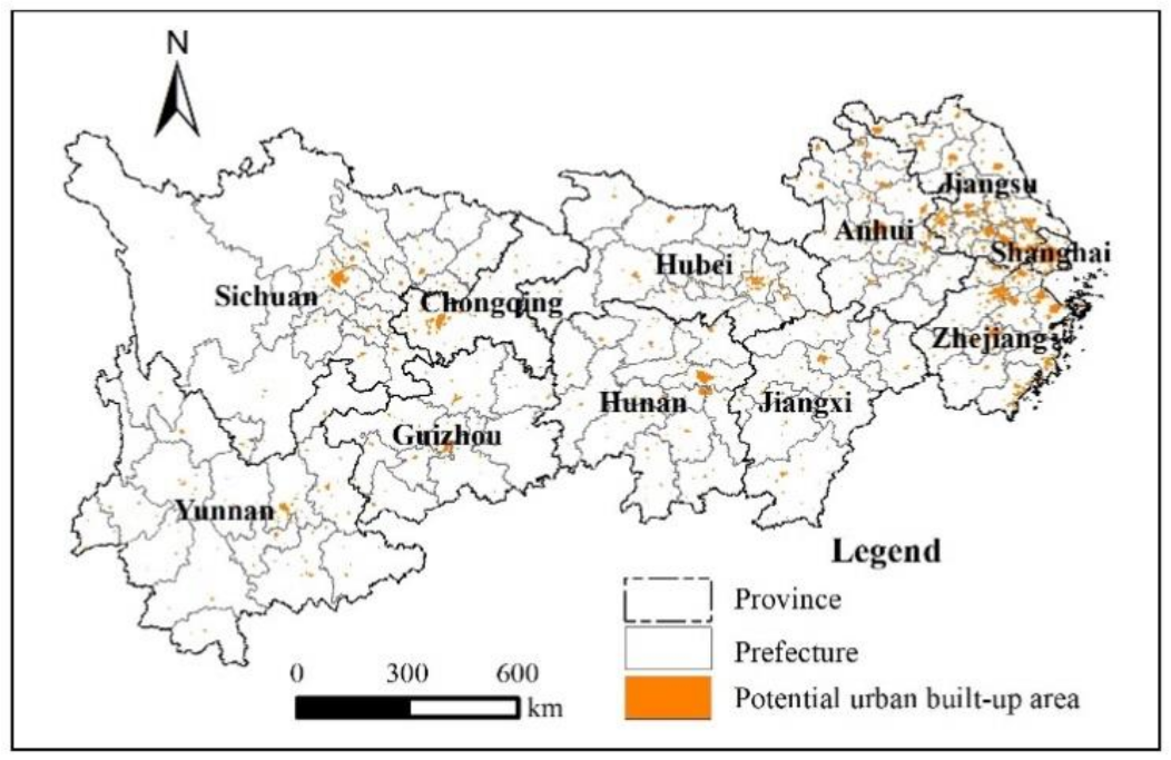
Figure 4.
The estimates of WSS for different k.

Figure 5.
Cluster results of potential urban clusters.
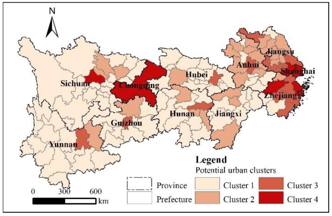
Figure 6.
The estimates of WSS for different k.
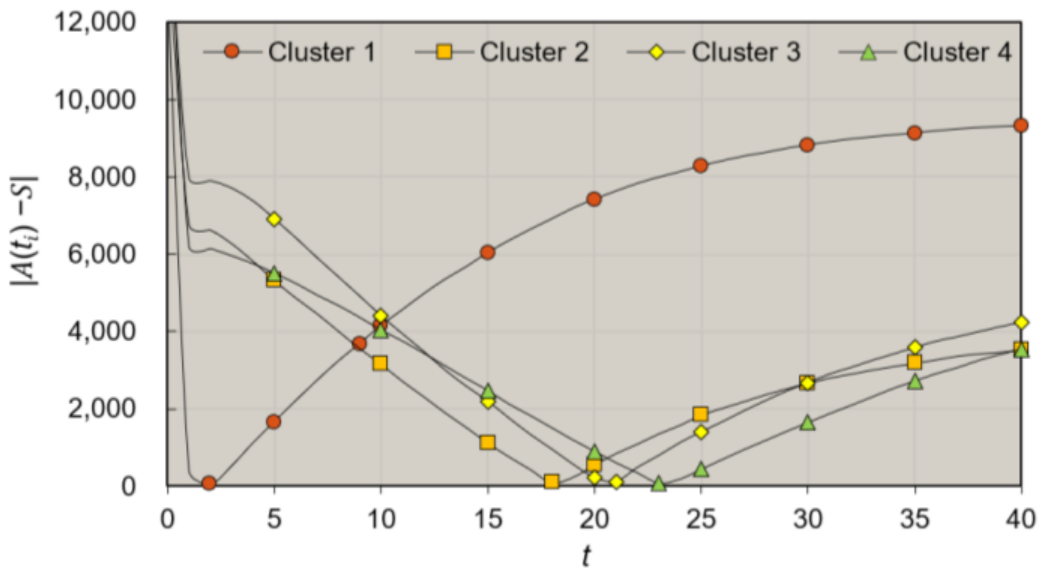
Figure 7.
Spatial distribution of urban and rural stations.
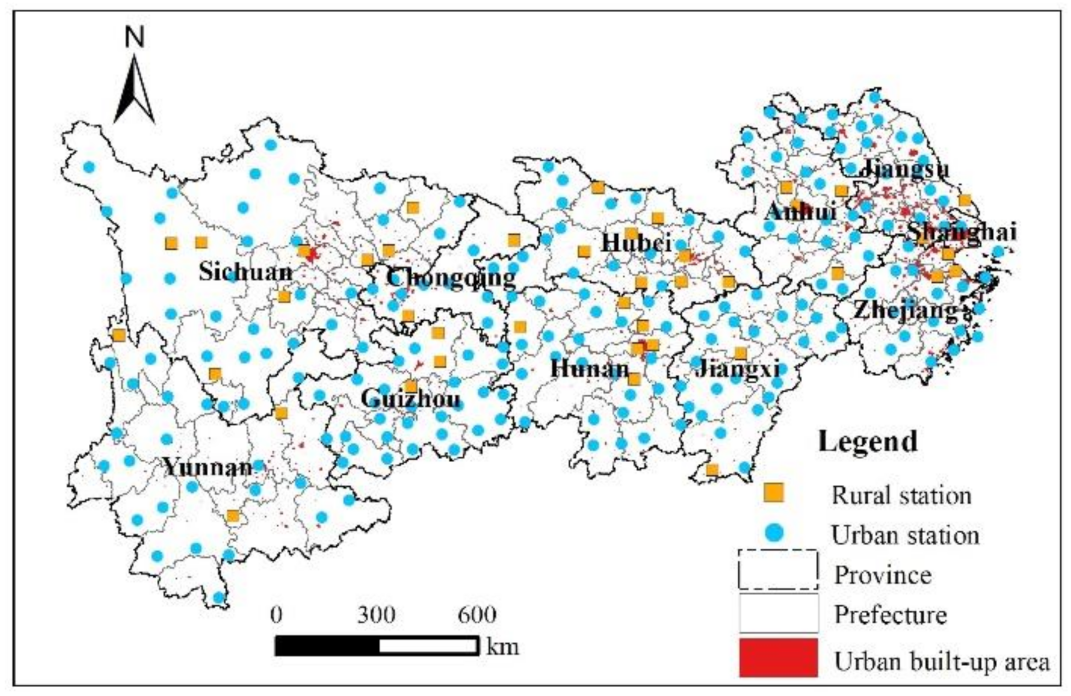
Figure 8.
Result of matching urban and rural stations based on 110 km buffer.
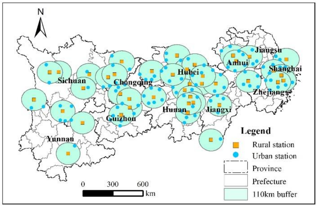
Figure 9.
Percentage of meteorological stations with different trends for the extreme temperature index.
Figure 9.
Percentage of meteorological stations with different trends for the extreme temperature index.

Figure 10.
Urbanization contribution rates of different extreme temperature indices: (a) TN90P, (b) TR20, (c) TNx, (d) TX90P, (e) TN10P, and (f) TX10P.
Figure 10.
Urbanization contribution rates of different extreme temperature indices: (a) TN90P, (b) TR20, (c) TNx, (d) TX90P, (e) TN10P, and (f) TX10P.
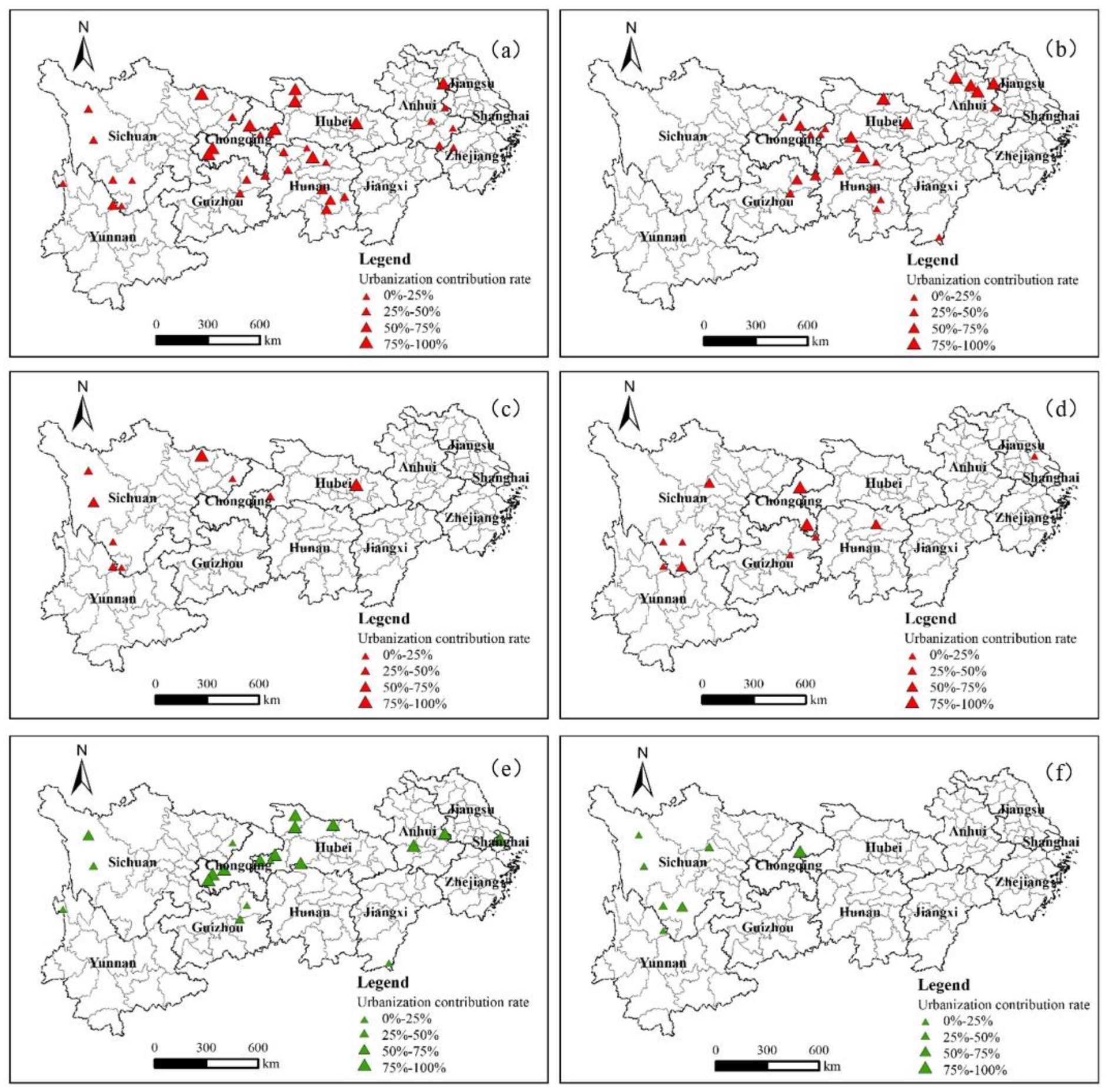
Figure 11.
Percentage of meteorological stations with different trends for the extreme precipitation index.
Figure 11.
Percentage of meteorological stations with different trends for the extreme precipitation index.

Figure 12.
Urbanization contribution rates of the extreme precipitation index Prcptot.


Table 1.
Extreme climate indices.
| Category | Index | Unit | Definition |
|---|---|---|---|
| Extreme temperature indices | FD0 * | day | Number of days with daily minimum temperature (TN) < 0℃ |
| ID0 * | day | Number of days with daily maximum temperature (TX) < 0℃ | |
| TN10P *, TN90P # | day | Number of days with TN < 10th (>90th) percentile | |
| TX10P *, TX90P # | day | Number of days with TX < 10th (>90th) percentile | |
| TR20 #, SU25 # | day | Number of days with TN > 20 ℃ (TX > 25 ℃) | |
| TNn, TNx/TXn, TXx | ℃ | Minimum (maximum) value of TN/TX | |
| DTR | K | Difference between TX and TN | |
| CSDI, WSDI | day | Number of days with TN < 10th (>90th) percentile for at least 6 consecutive days | |
| GSL | day | Numbers of days with daily average temperature>5℃ | |
| Extreme precipitation indices | SDII | mm/day | Annual precipitation divided by the number of wet days |
| CDD | day | Maximum number of consecutive days with daily precipitation amount (RR) < 1 mm (Maximum length of dry spell) | |
| CWD | day | Maximum number of consecutive days with RR ≥1 mm | |
| RX1day | mm | Maximum daily precipitation amount | |
| RX5day | mm | Maximum precipitation amount for 5 consecutive days | |
| R10mm, R20mm, R25mm | day | Number of days with RR > 10mm (20, 25 mm) | |
| R95P, R99P | day | Number of days with RR > 95th (99th) percentile | |
| Prcptot | mm | Annual precipitation amount |
# Warm indices: TN90P, TX90P, TR20, and Su25; * Cool indices: FD0, ID0, Ta10P, TN10P, and TX10P.
Publisher’s Note: MDPI stays neutral with regard to jurisdictional claims in published maps and institutional affiliations. |
© 2022 by the authors. Licensee MDPI, Basel, Switzerland. This article is an open access article distributed under the terms and conditions of the Creative Commons Attribution (CC BY) license (https://creativecommons.org/licenses/by/4.0/).
Share and Cite
MDPI and ACS Style
Yang, W.; Yan, Y.; Lin, Z.; Zhao, Y.; Li, C.; Zhang, X.; Shan, L. The Impact of Urbanization on Extreme Climate Indices in the Yangtze River Economic Belt, China. Land 2022, 11, 1379. https://doi.org/10.3390/land11091379
AMA Style
Yang W, Yan Y, Lin Z, Zhao Y, Li C, Zhang X, Shan L. The Impact of Urbanization on Extreme Climate Indices in the Yangtze River Economic Belt, China. Land. 2022; 11(9):1379. https://doi.org/10.3390/land11091379
Chicago/Turabian StyleYang, Wentao, Yining Yan, Zhibin Lin, Yijiang Zhao, Chaokui Li, Xinchang Zhang, and Liang Shan. 2022. "The Impact of Urbanization on Extreme Climate Indices in the Yangtze River Economic Belt, China" Land 11, no. 9: 1379. https://doi.org/10.3390/land11091379
Note that from the first issue of 2016, this journal uses article numbers instead of page numbers. See further details here.