
Spatio-Temporal Evolution and Influencing Factors of High Quality Development in the Yunnan–Guizhou, Region Based on the Perspective of a Beautiful China and SDGs


Abstract
:1. Introduction
2. Study Area and Data
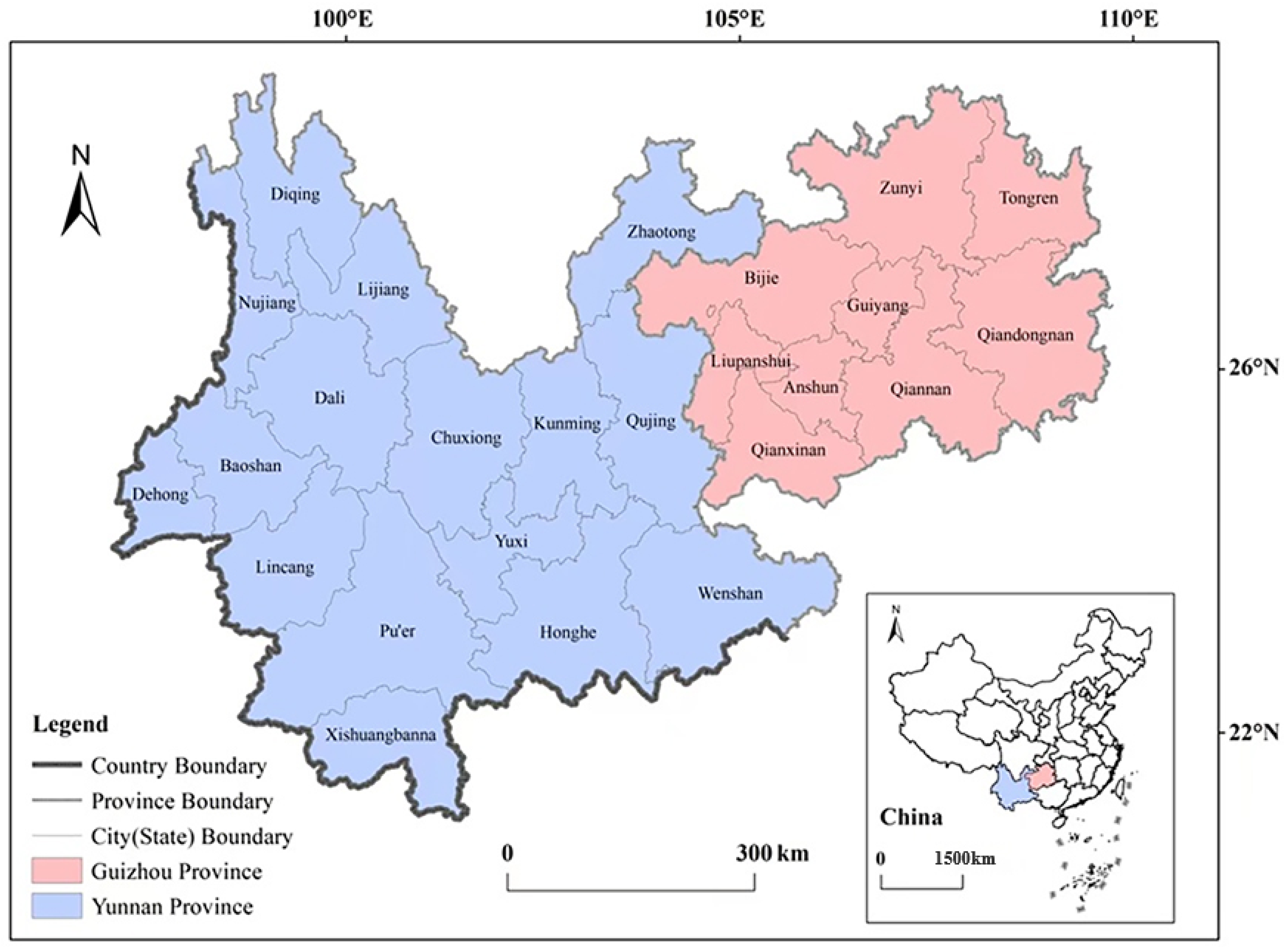
2.1. Study Area
2.1.1. Study Small Areas
2.1.2. Data Source
3. Research Method
3.1. Evolution Logic of Beautiful China, SDGs, and High-Quality Development
3.2. Construction of the Index System
3.3. The Entropy Weight–TOPSIS Model
- (1)
- Build a judgment matrix:
- (2)
- Normalize the judgment matrix to obtain the normalized matrix B.
- (3)
- According to the definition of entropy, determine the entropy of the evaluation in dex (H1):
- (4)
- The entropy weight of the evaluation index (W):
- (5)
- Find the weight set of each indicator [ ]:
- (6)
- Calculate the weight set according to the entropy weight method above (R), determining the ideal solution ( ), and determine the negative ideal solution ( ):
- (7)
- Calculate the distances and for each scheme from and :
- (8)
- Calculate the relative closeness of each scheme to the ideal solution (evaluation index):
3.4. Geographic-Weighted Regression (GWR)
4. Results and Analysis
4.1. Spatio-Temporal Pattern and Evolution Characteristics of the High-Quality Development of YGR
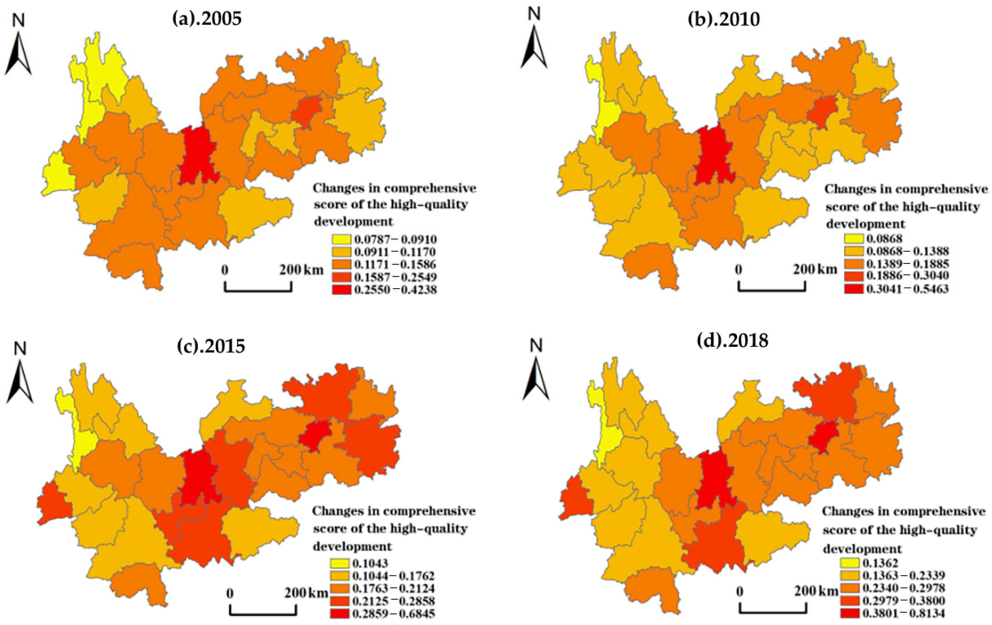
4.1.1. Characteristics of the Spatio-Temporal Pattern of the High-Quality Development of YGR
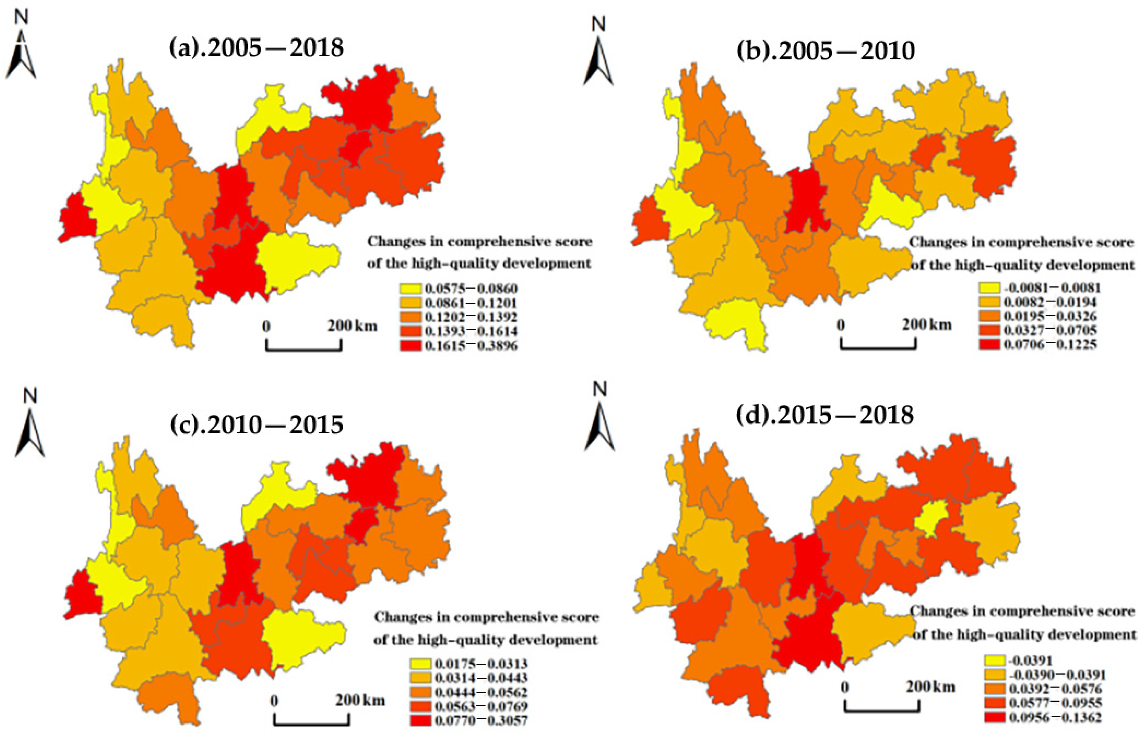
4.1.2. Characteristics of the Spatio-Temporal Evolution of the High-Quality Development of YGR
4.2. Identification of the Influencing Factors on the Spatio-Temporal Evolution of the High-Quality Development of YGR
4.2.1. Geographic Detection Results of the Influencing Factors
4.2.2. Spatial Differences in the Role of the Influencing Factors
- (1)
- The action model of the change in urban built-up areas
- (2)
- The action model of the change of per capita GDP
- (3)
- The action model of the change of total import and export
- (4)
- The action model of the change of tourism income
- (5)
- The action model of the change of total fixed asset investment
4.3. Quantitative Expression of Influencing Factors
- (1)
- The influencing factors
- (2)
- The strength of influencing factors
5. Discussion
5.1. Discussion on High Quality Development Level
5.2. Discussion on Influencing Factors
5.3. Limitations and Policy Implications
6. Conclusions
- (1)
- The high-quality development in the Yunnan–Guizhou area generally presents the spatial pattern of “central Yunnan–central Guizhou core dual drive” and “high east and low west”. In other words, Kunming and Guiyang have a higher development level. The high-quality development level of Guizhou province is higher than that of Yunnan province. In addition, the evolution speed of high-quality development in YGR generally presents the characteristics of “low speed–relatively high speed–high speed”.
- (2)
- The evolution of high-quality development in the YGR is mainly affected by the change of urban built-up area, per capita GDP, total foreign trade import and export, tourism income, and total fixed asset investment. The change of urban built-up area has both positive and negative correlation effects on the evolution of the development of the YGR in different time periods. The impact intensity generally decreased from west to east. Changes in per capita GDP and tourism income have positive correlated effects across all the time periods. The influence intensity decreased from north to south, and from west to east, respectively. The changes in total import and export and total fixed asset investment had negative correlation effects in a few cities at the early stage of the study. However, it gradually became a positive correlation effect for all the cities as the time increased. The influence intensity decreased from west to east and from center to east and west, respectively.
- (3)
- The five influencing factors on the evolution of high-quality development in the YGR have some differences in the mode and intensity of action in different time periods. Three forms exist in terms of action modes: dual factor enhancement, nonlinear enhancement, and the independent form. In terms of effect intensity, from 2005 to 2018, the change of total import and export and tourism income, had the strongest interaction. From 2005 to 2010, the interaction between the change of per capita GDP and tourism income was the strongest. From 2010 to 2015, the change of total import and export had the strongest interaction with the change of the total fixed asset investment. From 2015 to 2018, the change of tourism income had the strongest interaction with the change of the total fixed asset investment.
Author Contributions
Funding
Institutional Review Board Statement
Informed Consent Statement
Conflicts of Interest
References
- Hu, J. Unswervingly Advance along the Road of Socialism with Chinese Characteristics, and Strive to Build a Moderately Prosperous Society in an All-Round Way: A Report at the 18th National Congress of the Communist Party of China; Beijing People’s Press: Beijing, China, 2012. [Google Scholar]
- Ge, Q.; Fang, C.; Jiang, D. Geographical missions and coupling ways between human and nature for the Beautiful China Initiative. Acta Geogr. Sin. 2020, 75, 1109–1119. [Google Scholar]
- Xu, Z. How to understand China’s economy and related reforms after the 19th CPC National Congress. Shanghai Financ. 2018, 39, 1–4. [Google Scholar]
- Ma, R.; Luo, H.; Wang, H.; Wang, T.C. Study of evaluating high-quality economic development in Chinese regions. China Soft Sci. 2019, 34, 60–67. [Google Scholar]
- Yu, F.; Huang, X.; Yue, H. The high-quality development of rural tourism: Connotative features, key issues and countermeasures. Chin. Rural. Econ. 2020, 36, 27–39. [Google Scholar]
- Wei, H. Grasp the essence of integrated urban and rural development. Chin. Rural. Econ. 2020, 36, 5–8. [Google Scholar]
- Wang, W.; Wang, C. Evaluation and spatial differentiation of high-quality development in Northeast China. Sci. Geogr. Sin. 2020, 40, 1795–1802. [Google Scholar]
- Hua, X.; Jin, X.; Lv, H.; Ye, Y.; Shao, Y. Spatial-temporal pattern evolution and influencing factors of high quality development coupling coordination: Case on counties of Zhejiang Provinnce. Sci. Geogr. Sin. 2021, 41, 223–231. [Google Scholar]
- Sun, J.; Jiang, Z. Path of high-quality development in China’s coastal areas. Acta Geogr. Sin. 2021, 76, 277–294. [Google Scholar]
- Chen, Y.; Tian, W.; Zhou, Q.; Shi, T. Spatiotemporal and driving forces of Ecological Carrying Capacity for high-quality development of 286 cities in China. J. Clean. Prod. 2021, 293, 126186. [Google Scholar] [CrossRef]
- Li, J.; Shi, L.; Xu, A. Probe into the assessment indicator system on high-quality development. Stat. Res. 2019, 36, 4–14. [Google Scholar]
- Ou, J.; Xu, C.; Liu, Y. The measurement of high-quality development level from five development concepts: Empirical analysis of 21 prefecture-level cities in Guangdong province. Econ. Geogr. 2020, 40, 77–86. [Google Scholar]
- Liu, B.; Long, R.; Zhu, C.; Sun, X.; Pan, K. Comprehensive measurement of the index system for marine economy high-quality development in Jiangsu province. Econ. Geogr. 2020, 40, 104–113. [Google Scholar]
- Fang, Y.; Zhu, R. Strategic thinking on promoting high-quality development in upper reaches of the Yangtze River Economic Belt. Bull. Chin. Acad. Sci. 2020, 35, 988–999. [Google Scholar]
- Tu, J.; Kuang, R.; Mao, K.; Li, N. Evaluation on high-quality development of Chengdu-Chongqing urban agglomeration. Econ. Geogr. 2021, 41, 1–15. [Google Scholar]
- Wang, Q.; Ding, Y.; Guo, X. Construction of the indicator system of economic high-quality development of counties in China. Soft Sci. 2021, 35, 115–119, 133. [Google Scholar]
- Li, X.; Wen, Y.; Li, Y.; Yang, H. High-quality development of the Yellow River Basin from a perspective of economic georaphy: Man-land and spatial coordination. Econ. Geogr. 2020, 40, 1–10. [Google Scholar]
- Luo, Z.; Li, L.; Gao, X.; Zhang, Y. Study on the coupling and coordination of high-quality development and ecological environment of Lanzhou-Xining urban agglomeration based on the concept of ecological city. Res. Soil Water Conserv. 2021, 28, 276–284. [Google Scholar]
- People’s Government of Yunnan Province. Formulating the 14th Five-Year Plan for National Economic and Social Development and the Long-Term Goals for 2035 of Yunnan Province. 2022. Available online: http://www.yn.gov.cn/zwgk/zcwj/yzf/202102/t20210209_217052.html (accessed on 23 May 2022).
- People’s Government of Guizhou Province. Formulating the 14th Five-Year Plan for National Economic and Social Development and the Long-Term Goals for 2035 of Guizhou Province. 2021. Available online: http://www.guizhou.gov.cn/zwgk/zdlygk/jjgzlfz/ghjh/gmjjhshfzgh_5870291/202109/t20210913_70082489.html (accessed on 23 May 2022).
- Guo, X.; Li, X.; Cheng, D. Spatial distribution of temperature and precipitation and its influencing factors in the Yunnan-Guizhou Plateau. Res. Soil Water Conserv. 2021, 28, 159–163, 170. [Google Scholar]
- Chen, W.; Zhong, S.; Geng, Y.; Chen, Y.; Cui, X.; Wu, Q.; Pan, H.; Wu, R.; Sun, L.; Tian, X. Emergy based sustainability evaluation for Yunnan Province, China. J. Clean. Prod. 2017, 162, 1388–1397. [Google Scholar] [CrossRef]
- The Department of Statistics of Yunnan Province. Yunnan Statistical Yearbook 2005–2021. 2022. Available online: http://www.yn.gov.cn/sjfb/tjnj_2/ (accessed on 22 May 2022).
- The Department of Statistics of Guizhou Province. Guizhou Statistical Yearbook 2005–2021. 2022. Available online: https://www.guizhou.gov.cn/zwgk/zfsj/tjnj/ (accessed on 22 May 2022).
- National Bureau of Statistics. Chinese Urban Statistical Bulletin 2005–2021. 2022. Available online: http://www.stats.gov.cn/tjsj/ndsj/ (accessed on 22 May 2022).
- The Department of Ecology and Environment of Yunnan Province. Yunnan Environmental Bulletin 2005–2020. 2020. Available online: http://sthjt.yn.gov.cn/xxgk/xxgknb.aspx (accessed on 22 May 2022).
- The Department of Ecology and Environment of Guizhou Province. Guizhou Environmental Bulletin 2005–2020. 2020. Available online: https://sthj.guizhou.gov.cn/hjsj/hjzlsjzx_5802731/hjzkgb_5802732/szf_list.html (accessed on 22 May 2022).
- The Department of Water Resources of Yunnan Province. Yunnan Water Resources Bulletin 2005–2020. 2020. Available online: http://wcb.yn.gov.cn/html/shuiziyuangongbao/ (accessed on 22 May 2022).
- The Department of Water Resources of Guizhou Province. Guizhou Water Resources Bulletin 2005–2020. 2020. Available online: http://mwr.guizhou.gov.cn/slgb/slgb1/ (accessed on 22 May 2022).
- Cheng, Q.; Zhong, F.; Zuo, X.; Yang, C. Evaluation of water resources carrying capacity of Heihe River Basin combining Beautiful China with SDGs. J. Desert Res. 2020, 40, 204–214. [Google Scholar]
- Gao, F.; Zhao, X.; Song, X.; Wang, B.; Niu, Y.; Wang, W.; Huang, C. Connotation and evaluation index system of Beautiful Chinese for SDGs. Adv. Earth Sci. 2019, 34, 295–305. [Google Scholar]
- Zhu, J.; Sun, X.; He, Z. Research on China’s sustainable development evaluation indicators in the framework of SDGs. China Popul. Resour. Environ. 2018, 28, 9–18. [Google Scholar]
- Wang, T.; Zhang, J.; Yu, X.; Liu, B.; Chen, P. Sustainable development pathway of resource-based cities: A case study of Taiyuan innovation demonstration zone for national sustainable development agenda. China Popul. Resour. Environ. 2021, 31, 24–32. [Google Scholar]
- Fang, C.; Wang, Z.; Liu, H. Exploration on the theoretical basis and evaluation plan of beautiful China construction. Acta Geogr. Sin. 2019, 74, 619–632. [Google Scholar]
- Xie, B.; Chen, Y.; Li, X. The application of coupling coordination model in the evaluation of “Beautiful China” construction. Econ. Geogr. 2016, 36, 38–44. [Google Scholar]
- Wang, T.; Zhang, J.; Liu, B. Evaluation index system of National Innovation Demostration Zones for the 2030 Agenda for Sustainable Development. China Popul. Resour. Environ. 2020, 30, 17–26. [Google Scholar]
- Hu, Z.N.; Yang, X.; Yang, J.; Zhang, Z. Linking landscape pattern, ecosystem service value, and human well-being in Xishuangbanna, southwest China: Insights from a coupling coordination model. Glob. Ecol. Conserv. 2021, 27, e01583. [Google Scholar] [CrossRef]
- Cao, X.; Zeng, G. The mode of transformation and upgrading based on the methods of entropy weight and TOPSIS in case of Wuhu economic and technological development zone. Econ. Geogr. 2014, 34, 13–18. [Google Scholar]
- Cheng, Y.; Ren, J.; Cui, H.; Tang, G.M. A Research Using Entropy—Topsis Method on Regional Development Modes in Perspective of the Three-Dimensional Framework—A Case Study of Shandong Province. Econ. Geogr. 2012, 32, 27–31. [Google Scholar]
- Cao, X.; Wei, C.; Xie, D. Evaluation of Scale Management Suitability Based on the Entropy-TOPSIS Method. Land 2021, 10, 416. [Google Scholar] [CrossRef]
- Wang, J.; Xu, C. Geodetector: Principle and prospective. Acta Geogr. Sin. 2017, 72, 116–134. [Google Scholar]
- Han, J.; Rui, Y.; Yang, K.; Liu, W.; Ma, T. Quantitative attribution of national key town layout based on geodetector and the geographically weighted regression model. Prog. Geogr. 2020, 39, 1687–1697. [Google Scholar] [CrossRef]
- Powers, S.L.; Matthews, S.A.; Mowen, A.J. Does the relationship between racial, ethnic, and income diversity and social capital vary across the United States? A county-level analysis using geographically weighted regression. Appl. Geogr. 2021, 130, 102446. [Google Scholar]
- Shi, Y.; Li, X.; Meng, D. Evaluation of county industrialization process and analysis of spatial and temporal evolution in typical agricultural areas: A case study of Henan province. Econ. Geogr. 2020, 40, 118–126, 153. [Google Scholar]
- Zhang, H.; He, R.; Li, G.; Wang, J. Spatiotemporal evolution of coupling coordination degree of urban-rural integration system in metropolitan area and its influencing factors: Taking the capital region as an example. Econ. Geogr. 2020, 40, 56–67. [Google Scholar]
- Bai, J.; Zhang, H. Spatial-temporal analysis of economic growth in Central Plains Economic Zone with EOF and GWR methods. Geogr. Res. 2014, 33, 1230–1238. [Google Scholar]
- Wang, H.; Yan, J.; Wang, P.; Wu, Y. Spatial pattern of economic disparities in the multi-ethnic region of China. Resour. Environ. Yangtze Basin 2018, 27, 1525–1535. [Google Scholar]
- Liu, C.; Ma, Q. Spatial association network and driving factors of high quality development in the Yellow River Basin. Econ. Geogr. 2020, 40, 91–99. [Google Scholar]
- Gao, Z.; Ke, H. A comparative study on the high-quality development of economy in the border area of China. Econ. Rev. J. 2020, 36, 22–35. [Google Scholar]
- Wang, C.; Li, X.; Xie, Y.; Chen, P.; Xu, Y. Strategic path of Revitalization development of Northeast China under new era. Bull. Chin. Acad. Sci. 2020, 35, 884–894. [Google Scholar]
- Chen, Y.; Zhu, M.K.; Lu, J.L.; Zhou, Q.; Ma, W. Evaluation of ecological city and analysis of obstacle factors under the background of high-quality development: Taking cities in the Yellow River Basin as examples. Ecol. Indic. 2020, 118, 106771. [Google Scholar] [CrossRef]
- Xu, L.; Yao, S.; Chen, S.; Xu, Y. Evaluation of Eco-city Under the Concept High-quality Development: A Case Study of the Yangtze River Delta Urban Agglomeration. Sci. Geogr. Sin. 2019, 39, 1228–1237. [Google Scholar]
- Yang, K.; Pan, M.; Luo, Y.; Chen, K.; Zhao, Y.; Zhou, X. A time-series analysis of urbanization-induced impervious surface area extent in the Dianchi Lake watershed from 1988–2017. Int. J. Remote Sens. 2019, 40, 573–592. [Google Scholar] [CrossRef]


| Standard Floor | Elements Layer | Indicator Layer | Corresponding to the Beautiful China/Sustainable Development Evaluation System | Corresponding to the SDG Index | Class | Class | Weight |
|---|---|---|---|---|---|---|---|
| Resource load | Water resources utilization | Per capita water consumption/m3 | Peak et al. [31] | / | select | - | 0.0070 |
| Water consumption per unit of GDP/(m3·Wan Yuan−1) | Zhu Jing et al. [32]; Wang Tao et al. [33] | 6.4.1 | select | - | 0.0046 | ||
| Water consumption per unit of industrial added value/(m3·Wan Yuan−1) | Zhu Jing et al. [32] | 6.4.1 | select | - | 0.0032 | ||
| The sources of energy consume | Energy consumption per unit of GDP ab/(tce·Wan Yuan−1) | Fang Chuanglin et al. [34]; Zhu Jing et al. [32]; Wang Tao et al. [33] | / | select | - | 0.0044 | |
| Unit GDP power consumption/(kW h ten thousand yuan−1) | Fang Chuanglin et al. [34] | / | select | - | 0.0096 | ||
| Energy consumption per unit of industrial added value/(tce ten thousand yuan−1) | / | / | continue | - | 0.0026 | ||
| Land develop | Grain planting area/ten million ha | / | 2.4.1 | improve | + | 0.0391 | |
| highway mileage/km | Xie Binggeng et al. [35] | / | select | + | 0.0241 | ||
| Urban built-up area of/km2 | / | / | continue | + | 0.0629 | ||
| Economy develop | Economy actual strength | per capita GDP ab/first | Fang Chuanglin et al. [34]; Xie Binggeng et al. [35]; Zhu Jing et al. [32] | 8.1.1 | select | + | 0.0458 |
| GDP annual growth rate/% | Zhu Jing et al. [32] | 8.1.1 | select | + | 0.0143 | ||
| Industrial value added accounted for GDP a/% | Xie Binggeng et al. [35] | / | select | + | 0.0233 | ||
| Economy latent capacity | Science and technology expenditure accounts for/% of local fiscal expenditure | Fang Chuanglin et al. [34]; Wang Tao et al. [36] | 1.a.2 | select | + | 0.0485 | |
| The expenditure on education accounts for/% of the local fiscal expenditure | Fang Chuanglin et al. [34] | 1.a.2 | select | + | 0.0104 | ||
| R & D input strength ab/% | Zhu Jing et al. [32]; Wang Tao et al. [33] | 9.5.1 | select | + | 0.0550 | ||
| Economy vigor | Total foreign trade import and export volume ab/billions of dollars | / | / | select | 0.1730 | ||
| Tourism income b/100 million | / | 8.9.1 | improve | + | 0.0982 | ||
| gross fixed asset formation b/100 million | Xie Binggeng et al. [35] | / | select | + | 0.0765 | ||
| Organism’s habits environment protect | Environment foundation | land area covered with trees ab/% | √ Peak et al. [31]; Wang Tao et al. [33] | 15.1.1 | select | + | 0.0084 |
| Green coverage rate of the built-up area/% | Zhu Jing et al. [32]; Wang Tao et al. [33] | / | select | + | 0.0117 | ||
| Good air quality rate ab/% | √ Fang Chuanglin et al. [34]; Gao Feng et al. [31]; Wang Tao et al. [33] | / | select | + | 0.0061 | ||
| Environment pollute | Industrial sulfur dioxide emissions/t | Peak et al. [31]; Zhu Jing et al. [32] | / | select | - | 0.0074 | |
| Industrial wastewater discharge/million t | / | 6.3.1 | improve | - | 0.0045 | ||
| Agricultural chemical fertilizer application amount/t | √ Peak et al. [31] | / | select | - | 0.0059 | ||
| Environment administer | Urban domestic sewage treatment rate/% | √ Fang Chuanglin et al. [34]; Wang Tao et al. [33] | 6.3.1 | select | + | 0.0197 | |
| Comprehensive utilization rate of industrial solid waste/% | Peak et al. [31] | 11.6.1 | select | + | 0.0153 | ||
| Non-harmless treatment rate of urban household garbage/% | √ Fang Chuanglin et al. [34]; Wang Tao et al. [33] | / | select | + | 0.0149 | ||
| Society progress | Society harmonious | Urbanization rate ab/% | Fang Chuanglin et al. [34]; Xie Binggeng et al. [35]; Zhu Jing et al. [32] | / | select | + | 0.0210 |
| Urban-rural disposable income ratio b | Fang Chuanglin et al. [34]; Zhu Jing et al. [32]; Wang Tao et al. [33] | / | select | - | 0.0067 | ||
| The number of deaths in various production safety accidents b/human being | Zhu Jing et al. [32]; Wang Tao et al. [33] | 8.8.1 | select | - | 0.0092 | ||
| The people’s livelihood ensure | Registered urban unemployment rate ab/% | Zhu Jing et al. [32]; Wang Tao et al. [33] | 8.5.2 | select | - | 0.0082 | |
| Urban worker basic endowment insurance participation rate b/% | / | 1.3.1 | improve | + | 0.0487 | ||
| per capita output of grain ab/kg | Zhu Jing et al. [32] | 2.3.1 | select | + | 0.0119 | ||
| Public serve promote | Ten thousand people have the number of health technicians/person | Fang Chuanglin et al. [34]; Xie Binggeng et al. [35]; Zhu Jing et al. [32] | 3.c.1 | select | + | 0.0261 | |
| Ten thousand people have a middle school number/person | Fang Chuanglin et al. [34] | 4.1.2 | improve | + | 0.0158 | ||
| Internet penetration rate/% | Fang Chuanglin et al. [34]; Zhu Jing et al. [32] | 9.c.1 | select | + | 0.0560 |
| Particular Year | Urban Built-Up Area Change Value (X1) | Per Capita GDP Change Value (X2) | Total Import and Export Change Value (X3) | Tourism Income Change Value (X4) | Gross Fixed Asset Formation Change Value (X5) |
|---|---|---|---|---|---|
| 2005–2018 | 0.6346 | 0.6607 | 0.8518 | 0.7861 | 0.7930 |
| 2005–2010 | 0.6986 | 0.3931 | 0.6960 | 0.4040 | 0.7040 |
| 2010–2015 | 0.8030 | 0.7470 | 0.9046 | 0.7796 | 0.3992 |
| 2015–2018 | 0.2213 | 0.2329 | 0.7412 | 0.1634 | 0.5512 |
| Time | R2 | MAX (Cond) | MIN (Cond) |
|---|---|---|---|
| 2005–2018 | 0.9428 | 13.0260 | 9.8235 |
| 2005–2010 | 0.6228 | 19.4671 | 16.7829 |
| 2010–2015 | 0.9659 | 13.5091 | 9.5660 |
| 2015–2018 | 0.8852 | 10.3967 | 7.3962 |
| Each Other Factor | A Particular Year | Comparison of Interaction Values | Each Other Act on | Each Other Factor | A Particular Year | Comparison of Interaction Values | Each Other Act on |
|---|---|---|---|---|---|---|---|
| X1 ∩ X2 | 2005–2018 | 0.76 > Max[q (X1 = 0.63), q (X2 = 0.66)] | Double factor enhancement | X2 ∩ X4 | 2005–2018 | 0.87 > Max[q (X2 = 0.66), q (X4 = 0.79)] | Double factor enhancement |
| 2005–2010 | 0.75 > Max[q (X1 = 0.70), q (X2 = 0.39)] | Double factor enhancement | 2005–2010 | 0.89 > q (X2 = 0.39) + q (X4 = 0.40) | Nonlinear enhancement | ||
| 2010–2015 | 0.87 > Max[q (X1 = 0.80), q (X2 = 0.75)] | Double factor enhancement | 2010–2015 | 0.88 > Max[q (X2 = 0.75), q (X4 = 0.78)] | Double factor enhancement | ||
| 2015–2018 | 0.45 = q (X1 = 0.22) + q (X2 = 0.23) | independence | 2015–2018 | 0.75 > q (X2 = 0.23) + q (X4 = 0.16) | Nonlinear enhancement | ||
| X1 ∩ X3 | 2005–2018 | 0.91 > Max[q (X1 = 0.63), q (X3 = 0.85)] | Double factor enhancement | X2 ∩ X5 | 2005–2018 | 0.83 > Max[q (X2 = 0.66), q (X5 = 0.79)] | Double factor enhancement |
| 2005–2010 | 0.73 > Max[q (X1 = 0.70), q (X3 = 0.70)] | Double factor enhancement | 2005–2010 | 0.88 > Max[q (X2 = 0.39), q (X5 = 0.70)] | Double factor enhancement | ||
| 2010–2015 | 0.96 > Max[q (X1 = 0.80), q (X3 = 0.90)] | Double factor enhancement | 2010–2015 | 0.86 > Max[q (X2 = 0.75), q (X5 = 0.40)] | Double factor enhancement | ||
| 2015–2018 | 0.86 > Max[q (X1 = 0.22), q (X3 = 0.74)] | Double factor enhancement | 2015–2018 | 0.77 > Max[q (X2 = 0.23), q (X5 = 0.55)] | Double factor enhancement | ||
| X1 ∩ X4 | 2005–2018 | 0.87 > Max[q (X1 = 0.63), q (X4 = 0.79)] | Double factor enhancement | X3 ∩ X4 | 2005–2018 | 0.93 > Max[q (X3 = 0.85), q (X4 = 0.79)] | Double factor enhancement |
| 2005–2010 | 0.80 > Max[q (X1 = 0.70), q (X4 = 0.40)] | Double factor enhancement | 2005–2010 | 0.83 > Max[q (X3 = 0.70), q (X4 = 0.40)] | Double factor enhancement | ||
| 2010–2015 | 0.96 > Max[q (X1 = 0.80), q (X4 = 0.78)] | Double factor enhancement | 2010–2015 | 0.96 > Max[q (X3 = 0.90), q (X4 = 0.78)] | Double factor enhancement | ||
| 2015–2018 | 0.82 > q (X1 = 0.22) + q (X4 = 0.16) | Nonlinear enhancement | 2015–2018 | 0.89 > Max[q (X3 = 0.74), q (X4 = 0.16)] | Double factor enhancement | ||
| X1 ∩ X5 | 2005–2018 | 0.86 > Max[q (X1 = 0.63), q (X5 = 0.79)] | Double factor enhancement | X3 ∩ X5 | 2005–2018 | 0.92 > Max[q (X3 = 0.85), q (X5 = 0.79)] | Double factor enhancement |
| 2005–2010 | 0.81 > Max[q (X1 = 0.70), q (X5 = 0.70)] | Double factor enhancement | 2005–2010 | 0.76 > Max[q (X3 = 0.70), q (X5 = 0.70)] | Double factor enhancement | ||
| 2010–2015 | 0.87 > Max[q (X1 = 0.80), q (X5 = 0.40)] | Double factor enhancement | 2010–2015 | 0.98 > Max[q (X3 = 0.90), q (X5 = 0.40)] | Double factor enhancement | ||
| 2015–2018 | 0.79 > q (X1 = 0.22) + q (X5 = 0.55) | Nonlinear enhancement | 2015–2018 | 0.79 > Max[q (X3 = 0.74), q (X5 = 0.55)] | Double factor enhancement | ||
| X2 ∩ X3 | 2005–2018 | 0.92 > Max[q (X2 = 0.66), q (X3 = 0.85)] | Double factor enhancement | X4 ∩ X5 | 2005–2018 | 0.88 > Max[q (X4 = 0.79), q (X5 = 0.79)] | Double factor enhancement |
| 2005–2010 | 0.75 > Max[q (X2 = 0.39), q (X3 = 0.70)] | Double factor enhancement | 2005–2010 | 0.82 > Max[q (X4 = 0.40), q (X5 = 0.70)] | Double factor enhancement | ||
| 2010–2015 | 0.95 > Max[q (X2 = 0.75), q (X3 = 0.90)] | Double factor enhancement | 2010–2015 | 0.86 > Max[q (X4 = 0.78), q (X5 = 0.40)] | Double factor enhancement | ||
| 2015–2018 | 0.85 > Max[q (X2 = 0.23), q (X3 = 0.74)] | Double factor enhancement | 2015–2018 | 0.90 > q (X4 = 0.16) + (X5 = 0.55) | Nonlinear enhancement |
Publisher’s Note: MDPI stays neutral with regard to jurisdictional claims in published maps and institutional affiliations. |
© 2022 by the authors. Licensee MDPI, Basel, Switzerland. This article is an open access article distributed under the terms and conditions of the Creative Commons Attribution (CC BY) license (https://creativecommons.org/licenses/by/4.0/).
Share and Cite
Zhang, Z.; Hu, Z.; Zhong, F.; Cheng, Q.; Wu, M. Spatio-Temporal Evolution and Influencing Factors of High Quality Development in the Yunnan–Guizhou, Region Based on the Perspective of a Beautiful China and SDGs. Land 2022, 11, 821. https://doi.org/10.3390/land11060821
Zhang Z, Hu Z, Zhong F, Cheng Q, Wu M. Spatio-Temporal Evolution and Influencing Factors of High Quality Development in the Yunnan–Guizhou, Region Based on the Perspective of a Beautiful China and SDGs. Land. 2022; 11(6):821. https://doi.org/10.3390/land11060821
Chicago/Turabian StyleZhang, Zhuoya, Zheneng Hu, Fanglei Zhong, Qingping Cheng, and Mingzhu Wu. 2022. "Spatio-Temporal Evolution and Influencing Factors of High Quality Development in the Yunnan–Guizhou, Region Based on the Perspective of a Beautiful China and SDGs" Land 11, no. 6: 821. https://doi.org/10.3390/land11060821
APA StyleZhang, Z., Hu, Z., Zhong, F., Cheng, Q., & Wu, M. (2022). Spatio-Temporal Evolution and Influencing Factors of High Quality Development in the Yunnan–Guizhou, Region Based on the Perspective of a Beautiful China and SDGs. Land, 11(6), 821. https://doi.org/10.3390/land11060821