Article

Downscaling Switzerland Land Use/Land Cover Data Using Nearest Neighbors and an Expert System

1
EnviroSPACE Laboratory, Institute for Environmental Sciences, University of Geneva, Bd. Carl-Vogt 66, 1205 Geneva, Switzerland
2
GRID-Geneva, Institute for Environmental Sciences, University of Geneva, Bd. Carl-Vogt 66, 1205 Geneva, Switzerland
3
Agroscope, via A Ramél 18, 6593 Cadenazzo, Switzerland
*
Author to whom correspondence should be addressed.
Land 2022, 11(5), 615; https://doi.org/10.3390/land11050615
Submission received: 22 February 2022 / Revised: 12 April 2022 / Accepted: 20 April 2022 / Published: 21 April 2022

Abstract

:
High spatial and thematic resolution of Land Use/Cover (LU/LC) maps are central for accurate watershed analyses, improved species, and habitat distribution modeling as well as ecosystem services assessment, robust assessments of LU/LC changes, and calculation of indices. Downscaled LU/LC maps for Switzerland were obtained for three time periods by blending two inputs: the Swiss topographic base map at a 1:25,000 scale and the national LU/LC statistics obtained from aerial photointerpretation on a 100 m regular lattice of points. The spatial resolution of the resulting LU/LC map was improved by a factor of 16 to reach a resolution of 25 m, while the thematic resolution was increased from 29 (in the base map) to 62 land use categories. The method combines a simple inverse distance spatial weighting of 36 nearest neighbors’ information and an expert system of correspondence between input base map categories and possible output LU/LC types. The developed algorithm, written in Python, reads and writes gridded layers of more than 64 million pixels. Given the size of the analyzed area, a High-Performance Computing (HPC) cluster was used to parallelize the data and the analysis and to obtain results more efficiently. The method presented in this study is a generalizable approach that can be used to downscale different types of geographic information.

1. Introduction

1.1. Pressures on Land Resources in Switzerland

The Swiss Federal Department of Environment, Transport, Energy and Communications (DETEC) in its 2016 Strategy stated that by 2030, Switzerland is aiming at becoming a sustainable country while remaining an attractive and competitive business location with a high quality of life [1]. This ambitious objective is presently challenged by several trends such as population growth, increased mobility, energy demand, high consumption of resources, urbanization, loss of biodiversity and associated ecosystem services, and the digitalization of society along with related big data [2]. These trends have an important impact on the environment. Therefore, protecting the environment is a central mission for the Swiss Government, who wants to promote and adopt more sustainable approaches for the exploitation of natural resources [3]. To this end, actions such as protecting natural resources, improving urban planning, reducing emissions of greenhouse gases, preserving water quality, retaining biodiversity and ecosystem services, protecting soils, and preserving countryside are essential [4,5,6].
All these trends are also placing unprecedented demands on land. Between 1985 and 2009, 15% of the country’s surface area changed [7]. Settlement and urban areas have expanded, agricultural areas have been lost, forested areas have increased, and glaciers have receded [8,9,10]. During the last 50 years, it is estimated that human activities have affected globally about 83% of the terrestrial land surface and have degraded about 60% of services provided by ecosystems. Land degradation is now at a critical point and will undermine the well-being of 3.2 billion people by 2050 [11]. Consequently, Land Cover (LC) and Land Use (LU) changes are considered as a major tangible indicator of the human footprint [12].
To preserve its potential to deliver goods and services, land should be efficiently and sustainably managed. National policies such as the Green Economy, the Spatial Planning Act, the Spatial Strategy for Switzerland, the Sustainable Development Strategy 2016–2019, or the Strategy on Biodiversity are essential components to support this vision [13]. They generally acknowledge that a given area of land can offer many environmental, social, cultural, and economic benefits at once. However, most ecosystems are being degraded by unsustainable exploitation, fragmentation, urban growth and development of transport, and energy networks. This reduces the spatial and functional coherence of the landscape and consequently, degraded ecosystems are unable to provide the same services as healthy ecosystems [14].
Detailed and accurate knowledge on Land Use and Land Cover Change (LU/LCC) is crucial for many scientific and operational applications, such as watershed analyses [15,16], land use impact on stream ecology [17,18,19], species and habitat distribution modeling [20], dynamic modeling of species migration [21,22], reserve site selection [23], impact assessment on biodiversity [24], land use planning [25], or monitoring of land use changes [26]. LU/LC affects many aspects of policy and decision-making processes related to climate, water, biodiversity, ecosystems, agriculture, or disasters. Additionally, LU/LCC assessment also contributes to many Multilateral Environmental Agreements (MEAs) and Global Environmental Goals (GEGs) to guide and assess progress toward policy outcomes [27,28]. The importance of sustainable management of land resources is recognized in regional and global policies such as the 2030 Agenda for Sustainable Development, which contains land-related targets and indicators under 14 out of the 17 Sustainable Development Goals (SDGs) [29,30,31]. Many land organizations and stakeholders are committed to fully implement the SDGs and to monitor the land-related indicators to promote responsible land governance. Land is a significant resource for many sectors; timely and high-resolution LU/LC data therefore constitute critical information for the achievement of the SDGs [32]. Accurate and up-to-date LU/LCC information and related changes are also the base of a sustainable development assessment [33] based on structural (both temporal and spatial) and functional (social, ecological, economical) attributes of the landscape [34]. A supplementary challenge is represented by the spatial scale at which the assessment is performed. For each problem under study, an appropriate scale must be identified, especially when relating ecological processes to landscape patterns [35].

1.2. Land Use/Land Cover Data in Switzerland

LU/LCC is increasingly acknowledged as both a driver and a consequence of climate and biodiversity changes [36,37,38]. This important role has been featured by the fact that land cover is considered as an Essential Climate Variable (ECV), a supplementary Essential Water Variable (EWV), and a candidate Essential Biodiversity Variable (EBV) [39,40,41,42]. LU/LCC affects the biophysics, biogeochemistry, and biogeography of both the atmosphere and biosphere, with important consequences for human well-being. Consequently, accurate and timely information is necessary for understanding the impact of LU/LCC variations on the structure and functioning of ecosystems, as well as provision, support and regulation of goods and services [29,43,44]. However, it is recognized that inadequate information on LU/LC and its change over time is a recurrent and common problem that prevents policymakers from making sound, informed decisions [27,45,46,47]. Currently, the official LU/LC information in Switzerland (Arealstatistik) is updated approximately every 6 to 8 years and derived by visual interpretation of aerial photographs where an LC and an LU category are assigned to each intersection point of a regular 100 m grid [8]. Although this data set is very useful thanks to its thematic richness, neither its low spatial resolution nor the update frequency allow for providing accurate and timely information to depict and understand the dynamic of LU/LCC and the related impact across the country [48,49]. Accurate LU/LC change assessment and effective LU/LCC projections require higher spatial (e.g., 30 m) and temporal (e.g., yearly) data products to build consistent time series [47,50].

1.3. Downscaling as a Possible Approach for High-Resolution LU/LC Data

Besides traditional remote sensing approaches, such as unsupervised, supervised, or object-based classifications [51,52,53,54], more advanced techniques include machine or deep learning [55,56,57,58], new sensors with higher spatial and spectral resolution such as Sentinel-2 [59,60], and automated procedures to reduce the time-consuming process of manual verification of data [61,62]; a possible alternative to generate high-resolution LU/LCC data [63] is represented by downscaling techniques [64]. In many disciplines, downscaling is used to derive local scale maps from information available at coarser resolution. Climatologists refer to statistical downscaling [65] to describe this general approach that has been widely used not only for temperature and precipitation information [66,67] but also for wind speed [68] and air humidity [69]. In turn, downscaled climatic information is used in many different applications, such as hydrological modeling [70,71,72], species distribution modeling [73], and geological risk assessments [74]. However, downscaling of LU/LCC data is not very common and has not been widely applied [64,75,76].
Several statistical approaches have been used for downscaling. For instance, Barodssy et al. [77] used fuzzy rule-based models to predict frequency distributions of daily precipitation; Bürger and Chen [78] compared regression methods to derive river runoff from large-scale climatic scenarios; Biau et al. [79] used geostatistical methods (kriging) to estimate rainfall; and Coulibaly et al. (2005) [67] investigated the use of temporal neural networks to downscale temperature and precipitation.
Downscaling is not restricted to climatic data and has been used with remote sensing data to derive, for instance, soil moisture maps [80]. Species distribution modeling can also be defined as a general downscaling approach that predicts species distributions from point observations combined with spatially explicit environmental predictors [81]. The term “downscaling” can also be used when creating a land use map from combined input layers at various scales. For example, Remm [82] used case-based predictions to map the distribution of habitat classes from Landsat 7 ETM imagery, grayscale and color orthophotos, an elevation model, a digital base map, and a soil map.
Case-based algorithms are problem-solving methods that learn from experiences at a low level of generalization [83]. They can be considered as an Artificial Intelligence (AI) method that derives results from the data as directly as possible, without the formulation of an intermediate model. Machine learning (ML) specialists distinguish between lazy learning, which typically combines information during the problem-solving phase, and eager learning, which tends to derive a generalization and forget about raw observations after the learning phase [56,83,84]. Remm [82] argued that case-based methods represent a promising alternative for a large range of downscaling problems such as habitat mapping and the prediction of species’ potential distributions, especially with large and complex datasets where generalization is difficult.
Based on these considerations, the aim of this paper is to present a lazy learning method, which could be assimilated to a case-based approach, for downscaling LU/LC information for Switzerland from a 100 m lattice of points to a 25 m resolution grid, taking advantage of an existing 1:25,000 digital base map and building an expert system defining possible correspondences between the base map and the land use categories. This method is then applied for three different periods of time to assess land use and land cover change.

2. Materials and Methods

While land use and land cover maps are commonly derived from remote sensing or photointerpretation [85], traditional base maps of Switzerland have been available for more than a century and have been provided in digital format since the year 2000. LU/LC maps derived from the classification of remotely sensed images often have a “salt and pepper” appearance that does not meet end-user demand [26]. Land use derived from aerial photo interpretation can define many different classes of land use/cover categories, but the production is rather time-consuming. National base maps usually lack the thematic details that can be obtained from aerial photointerpretation but generally have an excellent geographic precision to define landscape patches and linear features. Hereafter will be presented the data inputs (Table 1), the downscaling methodology, and the expert system, together with its implementation and validation strategy.

2.1. Data Inputs

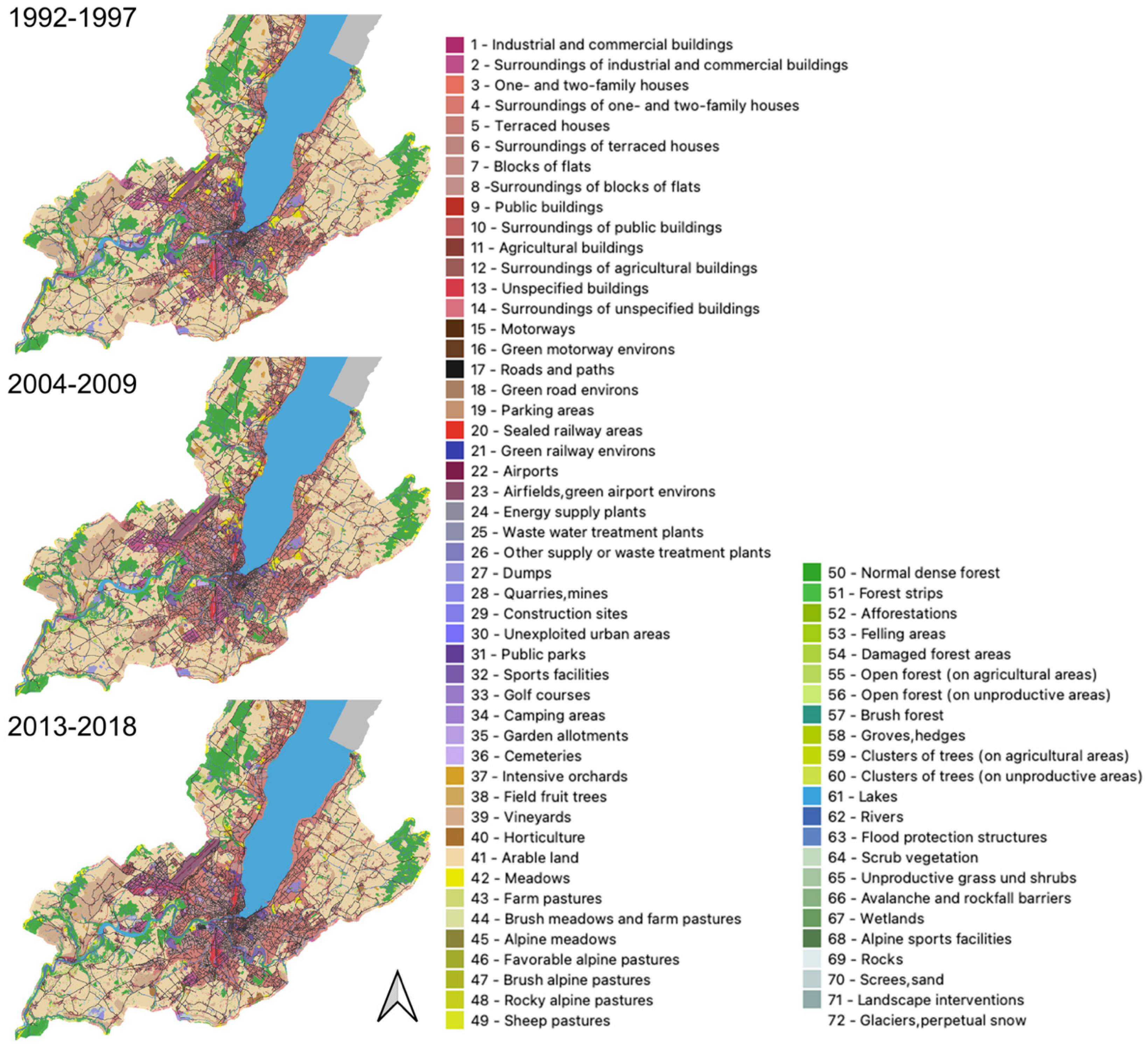
2.1.1. Land Use Statistics

LU/LC data are generated by visual interpretation of aerial photographs taken from a Federal Office of Topography (swisstopo)’s aircraft flying at an altitude of 5000 m and taking photos to regularly cover, over a 6-year period, the entire surface of Switzerland [8]. LU/LC maps are obtained by visually interpreting and assigning a LU/LC category to each point of a regular 100 m lattice laid over the Swiss territory, for a total of more than 4 million points over the country.There are three official classifications: (1) the standard nomenclature NOAS04 (72 basic categories which are a combination of LC and LU, 17 and 27 aggregation classes and 4 main domains); (2) the Land Cover nomenclature NOLC04 (27 basic categories and 6 main domains); and (3) the Land Use nomenclature NOLU04 (46 basic categories, 10 aggregation classes and 4 main domains). Three time periods are currently available (1979/85, 1992/97, 2004/09), and the latest version has just been finalized (2013/18) [7].
Strictly speaking, this dataset is not a LU/LC map, because its categories are assigned to points at the intersection of a 100 m grid rather than indicating the predominant LU/LC within each hectare square (Figure 1). It was developed as land use statistics over relatively large zones rather than as an LU/LC map per se. It tends, however, to be often used as an LU/LCC map in many applications [86] and remains the most exhaustive source of LU/LCC information for Switzerland. Even if this dataset is thematically more precise than the classification commonly used in Europe—the Coordination of Information on the Environment Land Cover (CORINE Land Cover, CLC), which has 44 classes [87]—it suffers from a low spatial and temporal resolution. Indeed, LU/LC units are coarse with a spatial resolution of 1 hectare, and a lot of information is therefore aggregated with a large degree of generalization. Consequently, various landscape features, qualities, particularities, and configurations cannot be correctly represented.

2.1.2. National Base Map (Land Cover)

The Swiss Federal Office of Topography (swisstopo) provides digital versions of national topographic base maps at a 1:25,000 scale as a landscape model in a vector format. The data model used until 2011 was called Vector 25 and was later replaced by the Swiss Topographic Landscape Model (TLM3D). Both include millions of natural and artificial landscape features, together with their position, shape, type and many other attributes [88]. This land cover information is defined in 29 categories (Figure 2). Data on linear features such as rivers, roads and rails can also be obtained separately. The national base maps (TLM3D) are the geographically most precise source of land cover information for the entire country with a geometric accuracy for different landscape features between 0.2 m and 3 m that is partially updated every year.

2.1.3. Resolution

For the analysis, all available datasets were rasterized either at a 25 m and/or at a 100 m resolution to allow raster overlays. With a surface of 42,000 km2, Switzerland can be described with approximately 4 million pixels at a 100 m resolution and with 64 million pixels at a 25 m resolution.

2.1.4. Data Quality of Inputs

The two main data inputs of this study are of the highest possible quality from the two main national producers of geospatial data. The first one, land use statistics, has been developed by the Swiss Federal Office of Statistics with state-of-the-art photointerpretation methods, resulting in a very high quality of thematic resolution in the selection of land use classes on each hectare point of the country. The second input, the national base maps, are produced by the Swiss Federal Office of Topography and represent the official geographic representation of the country at a 1:25,000 scale with very high spatial accuracy but a less developed thematic resolution than the first input.

2.2. Downscaling Algorithm and Expert System

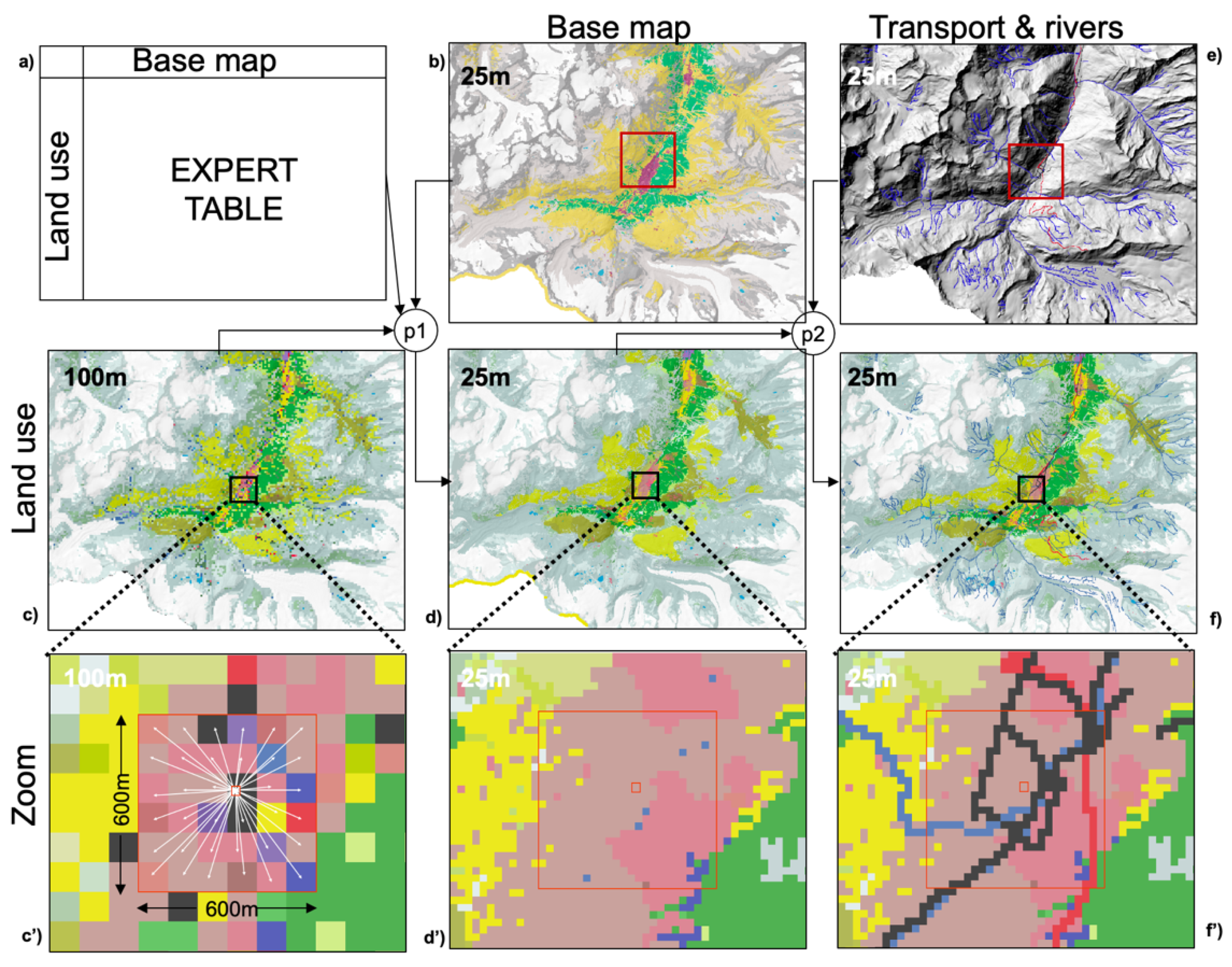
2.2.1. Downscaling Algorithm

The approach used for downscaling the existing land use information from 100 to 25 m relies on both the geographic precision of the 1:25,000 national topographic base map rasterized at 25 m and the detailed LU/LC categories obtained from the land use statistics available at 100 m. The developed algorithm uses inverse distance weighting combined with an expert system to assign reasonable land use categories at a finer scale (Figure 3).
The main steps of the downscaling methodology are the following (data preparation: 1–2–3; process [1] of downscaling: 4–10; process [2] for linear features: 11):
  • Rasterize a land use grid at 100 m resolution from the lattice of points of the land use statistics (Landuse100).
  • Convert to Non-Applicable (NA) land use categories that correspond to linear features (rivers, roads, rails).
  • Rasterize the primary surfaces of the land cover vector base map at a 25 m resolution (BaseMap25).
  • Visit each BaseMap25 pixel (target pixel).
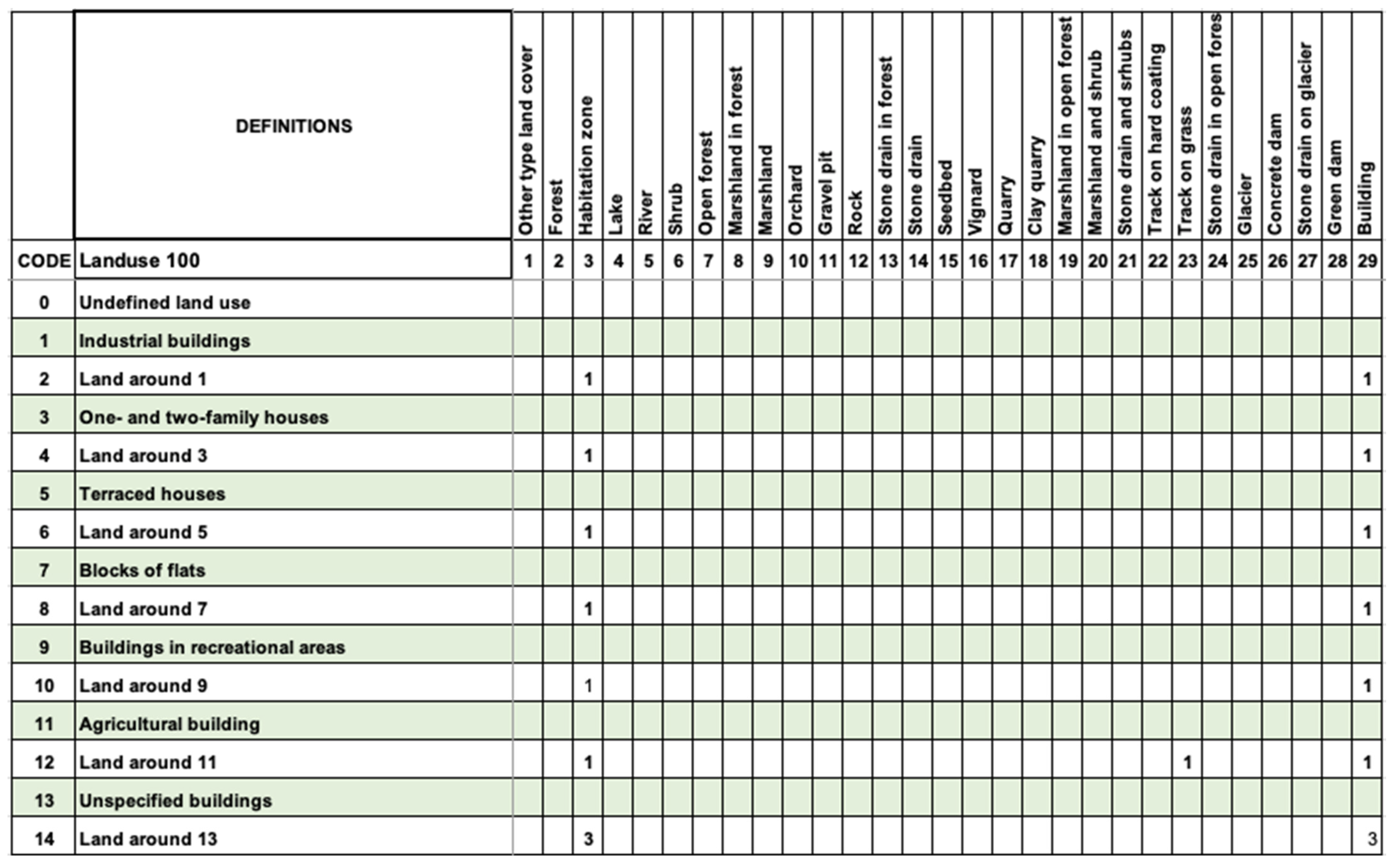
  • Then, according to the expert system table (Figure 4), select the land use categories that could be eligible for the target pixel. In some rare cases, assign the only possible category (then go to point 10).
  • Select among the 36 nearest Landuse100 neighbors those with eligible categories.
  • Calculate the inverse distance to each neighbor.
  • Sum up the inverse distances for each category.
  • Assign to the BaseMap25 pixel the category obtaining the higher score or, in case of lack of decision, assign the best replacement choice according to the expert system table.
  • Repeat steps 4 to 9 for each BaseMap25 pixel.
  • Replace categories wherever river, road, or rail linear features are available from BaseMap25. Only main roads (>3 m wide) and main railways were considered without tunnels and bridges. Underground rivers were ignored. Rivers, railways, roads, and freeways were rasterized at 25 m and added in this order after the first phase of downscaling.
The Inverse Distance Weighting (IDW) calculates a scaled distance to each of the 36 Landuse100 neighbors around the pixel under investigation, and does so in two spatial dimensions (Equation (1)):
dj(i) = sqrt((x25ix100j)2 + (y25iy100j)2)/maxrange
where j spans from 1 to 36 nearest neighbors and i represents each visited pixel at a 25 m resolution and maxrange the maximum distance between these pixels.
Then the inverse distances are summed up by land use category (Equation (2)):
D k ( i ) = j = 1 36 ( λ j ( k ) d j ( i ) + s )
where λ j ( k ) = { 1   i f   l a n d u s e t y p e j = k 0   o t h e r w i s e , and s is smoothing factor.
Finally, the category scoring the highest sum of inverse distances is assigned to the pixel under investigation (Equation (3)):
K ( i ) = g r e a t e s t k ( D k ( i ) )
IDW is generally used for interpolating cardinal discrete values (e.g., temperatures, precipitations) but can be also used on nominal values to spatially interpolate missing LC data [89], create super-resolution LC maps [90], or rescale LC data [91]. IDW assumes that values that are close to one another are more similar than those that are at a greater distance. In the proposed method, measured values surrounding the prediction location are considered but then they are spatially weighted (i.e., taking into account the distance of each pixel and the frequency of classes) and constrained (i.e., by the expert system). Consequently, the proposed downscaling method is filling a geographically very precise map (the base map) with information on the most plausible LU/LC category found in the neighborhood by reducing the possible choices with an expert table. This approach has the advantage of fully respecting the geographical quality of the base map while enriching it with a better thematic resolution.

2.2.2. Expert System

An expert system was used to constrain the possible choices when using information from BaseMap25 to select the most appropriate Landuse100 category (Figure 4). For instance, if a forest patch is defined for a particular site in BaseMap25, the expert system constrains the choice of Landuse100 categories to include only those related to forest. Furthermore, the expert system can also select a default Landuse100 category when the distance-based algorithm fails to make a clear selection because of the lack of eligible land use categories within the searching neighborhood.

2.3. Implementation

Although the algorithm used is relatively simple, it requires extensive calculations on several large grids (25 m resolution grid for Switzerland contains approximately 64 million pixels), which is time-consuming. To ensure the portability of the code on different platforms, the algorithm has been implemented using a set of open-source software and libraries. The programming language is Python 3 [92] using the PyCharm Community Edition (CE) Integrated Development Environment (IDE) [93]. The implemented algorithm relies on the following libraries: (1) the Geospatial Data Abstraction Library (GDAL) [94] to handle raster data; (2) Numpy [95] and math for mathematical operations on large multi-dimensional arrays; and (3) xlrd [96] and pandas [97] for reading and formatting information from Excel files.
To ensure a fast and efficient processing, the algorithm has been parallelized and executed on the High-Performance Computing cluster at University of Geneva [98], allowing to process the entire 64 million pixels grid significantly faster. The analyzed area is subdivided in tiles and the processing of each tile is performed on a different node on the cluster. The surface of Switzerland was divided in 900 tiles (30 × 30), which were associated to 900 jobs in the cluster, using SLURM job arrays. The processing time is on average less than 2 h per tile, but the actual processing time of a single tile is strongly dependent on the user priority and on the cluster load at the execution time. When the results of all the jobs are available, a final script is launched to assemble the 900 processed tiles together in a single image.
The code is freely available on GitHub [99] under an Apache 2.0 license, and a static version can be downloaded from the University of Geneva digital repository [100] under a CC-BY 4.0 license.

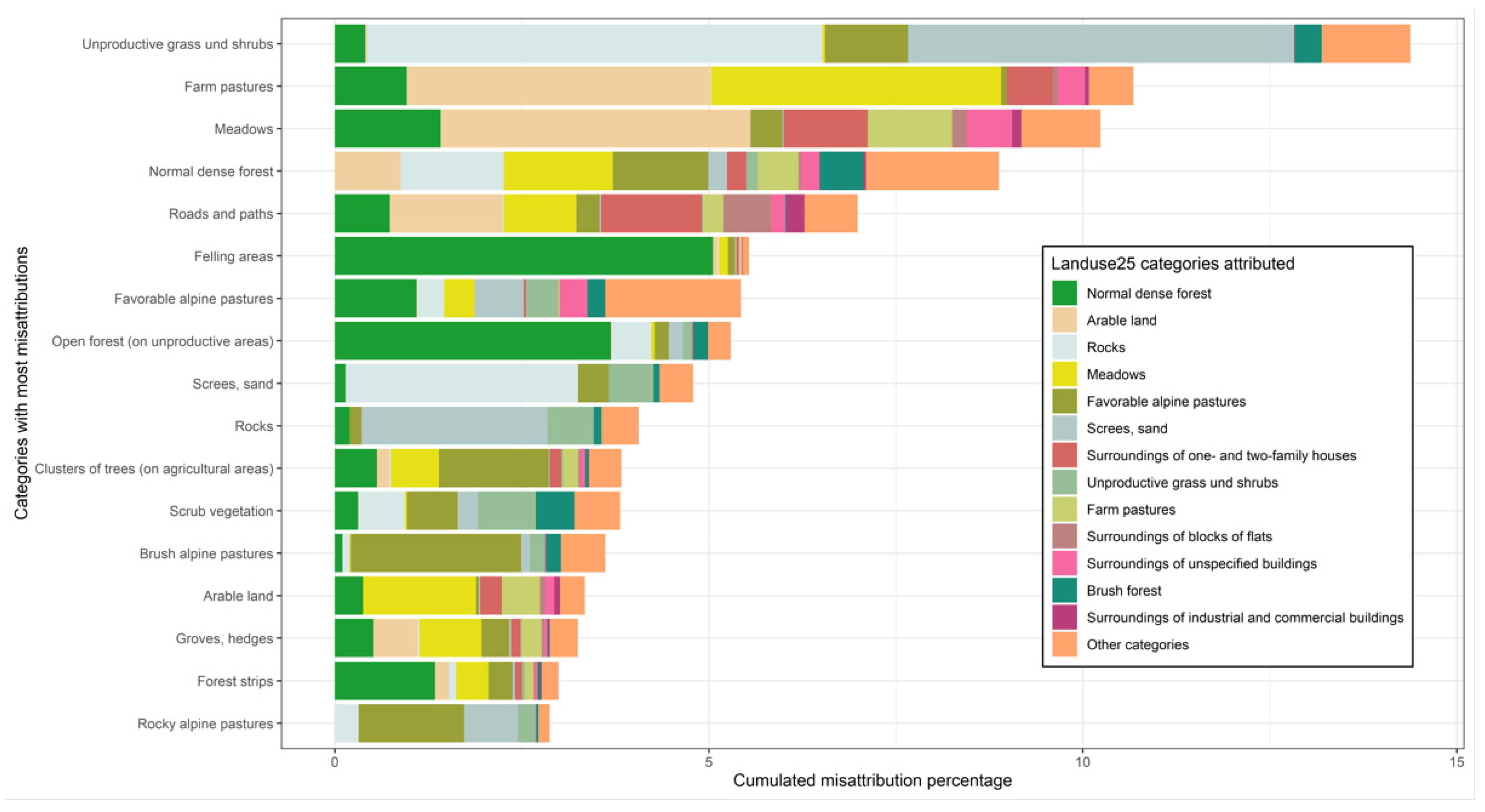
2.4. Validation and Accuracy Assessment

The categories of the downscaled LU/LC maps at 25 m (with or without linear features) for the three periods were compared with the categories of the original LU/LC point statistics. A random sample of 500,000 out of 4,129,070 points was used for this assessment. Multi-class classification metrics were used to assess the efficiency of the algorithm to classify each LU/LC category [101,102,103]. Results are shown as F1-score, which is obtained by harmonic mean from the recall and precision, and Cohen’s kappa coefficient [104]. Results were expressed as class F1-scores and weighted means for each dataset, and kappa coefficient for each dataset. Barplots and boxplots are used to display these metrics and the main misclassifications per category. The relative surface area per category was also compared to that of the original Landuse100 dataset [64,105].

3. Results

Results from the land use downscaling are best appreciated at a regional scale (Figure 5 and Figure S1), where the map produced by the algorithm not only preserves the geographic precision of the original BaseMap25 map but also inherits the higher definition of categories (66 categories in the downscaled map compared to 29 categories in BaseMap25). Seventy-two categories were originally found in Landuse100, but a few groupings had to be performed on some less important categories (e.g., buildings and their surroundings). The new map has a much finer grain and can be used for Geographical Information System (GIS) overlays at much finer scales, where the 16-fold increase in the density of pixels gives substantially improved results. Fine-scale details on roads and river networks were also maintained, whereas they are often difficult to represent adequately in coarse resolution raster formats (Figure 6).
The average percentage of similarity for the three periods evaluated between the original points found in the Landuse100 statistics and the resulting Landuse25 classifications is 71% when assessed without roads, rivers, and rails, and 68% when assessed with these linear features. Several categories have a correspondence of 70% or greater. Overall F1-scores and kappa coefficient are high (0.69 and 0.67, respectively). Individual classes F1-scores range from 0.007 to 0.98 depending on the category (Figure 7). Weighted mean F1-scores per dataset range from 0.67 to 0.70. Kappa scores range from 0.65 to 0.69. Categories from the Landuse100 classification that show zero correspondence are those that were not predicted, such as flood protection structures (63), field fruit trees (38), or grooves and hedges (58), and were thus discarded from the validation analysis. The categories that are best respected by the downscaling are those that have a large spatial representation and those that were imposed from the topographic map.
The percentages of misclassification for the downscaling of 2018 without linear features are represented in Figure 8. The major misclassifications concern unproductive grasslands (15%), farm pastures (12%), and meadows (10%). The classes in which the pixels were misattributed are also presented (color in the box). This figure will help in understanding the behavior of the downscaling algorithm to further improve it.
The absolute surface area difference from the downscaled map (Landuse25) categories compared to the original Landuse100 map ranges from −87,585 ha for the category “unproductive grass and shrubs” to +118,174 ha for the category “normal dense forest” (Figure 9). On average, a difference of 532 ha per category is observed. Underlaying reasons for large discrepancies in surface areas (misattributed categories) are further displayed in Figure 8. The relative surface area difference (proportion from downscaled map compared to original) ranges from −100% for small categories that were not included in the algorithm to +355% for cat. 14, “surroundings of unspecified buildings”.

4. Discussion

The method presented in this study is a generalizable approach that can be used to downscale different types of geographic information such as results from photo interpretations, classifications of remotely sensed images, or vegetation and soil maps. The general idea is to use the nearest precise point observations to define the attribute of a target pixel at a finer resolution within an area defined by a high-resolution land cover map. Other co-variables such as remote sensing indices (e.g., Normalized Difference Vegetation Index (NDVI)), topographic position, slope, or orientation could also be used to help model the most probable LU/LC category and could certainly further improve the present method.
In the case study presented here, the use of a national topographic base map at a 1:25,000 scale to define main land cover patches guarantees a perfect overlay with official maps. Indeed, topographic base maps are now available in digital format and are widely used as reference maps in most studies and field work. The possibility of matching the geometry defined by base maps with detailed land use categories reinforces the chance of uptake from end-users. However, some recent changes in LU/LC that might be visible from remote sensing images could be lost if involving changes between incompatible land use categories as defined by the expert system.
One of the main strengths of the proposed approach is that it avoids the “salt and pepper” effect generally resulting from the classification of remotely sensed images [26], except in the case of object-oriented classifications [106]. We believe that our approach could be particularly useful in this respect and could be used to smooth out land use maps obtained from remote sensing classifications. In such a case, land use statistics would be replaced by the land use classification obtained from supervised or unsupervised classification of the remotely sensed image, whereas the land cover information would still be retrieved from the national base map. Moreover, with the increased spatial resolution and the removal of the “salt and pepper” effect, LU/LC changes are more evident and can be assessed more easily (Figure 10).
The proportion (71%) of exact matches between the land use categories recorded at the 100 m resolution lattice points of the Landuse100 statistics and the corresponding points in the downscaled map (25 m resolution) is particularly encouraging. Discrepancies appear to result mainly from the change in scale and geometric precision brought in by the 1:25,000 base maps. The fundamental difference in approach between the land use statistics (punctual) and the topographic map (surface) is also important. A visual check confirms that most divergences mainly occur along boundaries of patches of different land use and along linear and small features. By using an inverse distance calculation—which gives a higher weight to close-by information—to choose the best land use category for each pixel, we greatly favored the retaining of input land use categories at an observed location in the result. This effect can be modulated by the smoothing factor in Equation (2).
The approach could be used at even finer scales by rasterizing for instance the topographic maps at 10 m instead of 25 m or using a regional map at a finer scale (1:10,000). Getting accurate land use information is crucial for calculating landscape indices such as those obtained from FRAGSTAT [107]. As demonstrated by Uuemaa et al. [108], changing grain size can have a significant effect on many landscape metrics. Therefore, one should pay attention to the scale at which a given landscape metric is calculated, and what grain size of land use maps is best adapted for the purpose, as there is no single land use scale which is “best” for observing and managing changes in land use patterns.
The implementation of a case-based reasoning algorithm in Python code proved to be a very efficient approach given the very large number of pixels (64 million) to handle but required the development of a purpose-written software. The availability of tools for implementing case-based approaches within existing GIS packages would certainly be very useful for many applications. One such tool has been developed by Remm [82] using Microsoft Visual Studio.NET, and this can predict several response types (binomial, multinomial, continuous, and complex) based on continuous and categorical predictors.
Riitters [109] mentions the practical trade-off that exists between the generality, precision, and realism of a method, as previously proposed by Levins [110], and emphasizes that generality and realism should be maximized at national scales, while precision should be optimized at local scales. Indeed, the use of the same raw data to develop models at different scales will enhance thematic and geographic comparisons between disciplines and across scales. Methods to upscale and downscale data are therefore central to local, national, and global environmental assessments.
The presented approach contributes to tackle the need of increased spatial resolution of LU/LCC information. However, the temporal issue remains a major problem. Indeed, land cover changes are caused by either natural or anthropogenic sources such as climate change, demographic growth, and economic growth [111,112]. Therefore, the state of land cover is highly dynamic and involves an inherent challenge for its mapping and monitoring that remains not adequately addressed [85]. Timely and reliable information on land cover change is crucial to efficiently mitigate the negative impact of environmental changes [113,114]. Traditional environmental data collection (e.g., field data collection) suffers from many shortcomings, among them the data inconsistency caused by changes in reporting methodologies through time, the gaps (missing measurements) in data series, and the fact that it is notoriously time-consuming and labor-intensive [115]. One of the main advantages of remotely sensed data collection is that it can provide a synoptic and repetitive view of a given area/region. With the opening of different Earth Observations (EO) data archives such as Landsat [112,116,117], it becomes possible to build consistent time series (i.e., image of the same location at regular intervals) to compare different periods of time and derive trends [118,119,120].
At the national scale, various attempts have been made to use satellite imagery, but unfortunately, no processes are currently in place to routinely generate accurate, consistent, and regular LU/LCC data. These large volumes of freely and openly available EO data are still underutilized and are not effectively used for national environmental monitoring. Therefore, mapping and monitoring LU/LC changes remain as challenges that are not adequately addressed at the national scale, and new methodologies are required to produce consistent and reliable yearly, medium-to-high-resolution (spatial, temporal, thematic) time series of LU/LCC data and projections of their (future) change across Switzerland to inform national and regional environmental policies and planning.
With the opening of different medium-to-high-resolution satellite EO data archives such as Landsat or Copernicus and the development of advanced data science techniques (e.g., Big Data, Artificial Intelligence, High-Performance Computing), it now becomes possible to build consistent time series of LC, to investigate the spatio-temporal dynamics of LC, and to perform quantitative assessments of LC dynamics, by comparing different periods of time, deriving trends, and determining environmental trajectories [121]. This can generate a consistent and reliable LU/LC time series that will help to understand the evolution of LU/LCC in Switzerland over the last 30 years and to model future changes according to plausible scenarios by 2050 [122,123].
To reach this objective, an essential pre-condition to support user applications and generate usable information products is to facilitate data access, preparation, and analysis. The systematic and regular provision of Analysis-Ready Data (ARD) can significantly reduce the burden of EO data usage. To be considered as ARD, data should be processed according to a minimum set of requirements (e.g., radiometric and geometric calibration; atmospheric correction; metadata description) and organized in a way that allows immediate analysis without additional effort [124,125]. In Switzerland, more than 37 years of satellite EO Analysis-Ready Data over Switzerland are made available by the Swiss Data Cube [126,127]. The increasing availability of EO data together with the improved computing and storage capacities allow monitoring, mapping, and assessing LU/LC and its change over time on large areas in a consistent and reliable manner. This favors the development of annual, high-quality LU/LC products based on time series data and can inform on class stability and transitions [128].

5. Conclusions

The proposed downscaling approach allowed for combining the geographic precision of existing topographic base maps with the thematic details of photo-interpreted land use statistics. Improved land use maps open the door to more accurate watershed analyses, species and habitat distribution modeling, and species dynamic models of migration. Accurate land use information is also the base for developing sustainable development indicators defining the structural and functional attributes of landscapes.
The proposed approach could be implemented for three time periods. It allowed for an efficiently downscaled LU/LC at a spatial resolution that is more suitable for environmental change monitoring. The increased spatial resolution removed the “salt and pepper” effect, and consequently, LU/LC changes are more evident. However, the changing definition of the base map input across the years resulted in discrepancies in the resulting downscaled maps that are refraining their use for land use change analyses. We therefore recommend using the original land use statistics data for trend analyses and our downscaled data for GIS analyses at each time period. The presented approach contributes to tackling the need for increased spatial resolution of LU/LC information, but the temporal issue is still a major problem. The use of dense time series of satellite data such as those provided in the Swiss Data Cube can be a promising solution to investigate to obtain high spatial and temporal LU/LC data over the country.

Supplementary Materials

The following are available online at https://www.mdpi.com/article/10.3390/land11050615/s1. Figure S1. Final result of the downscaled Land Use/Land Cover at 25 m for the period 2013/18. Table S1. Full version of the expert table.

Author Contributions

Conceptualization, A.L. and R.M.; methodology, A.L.; software, A.L., G.G. and D.R.; validation, A.L. and N.K.; formal analysis, A.L., G.G. and D.R.; data curation, A.L. and N.K.; writing—original draft preparation, G.G., A.L. and R.M.; writing—review and editing, all; visualization, A.L. and N.K.; supervision, A.L.; project administration, A.L.; funding acquisition, A.L. All authors have read and agreed to the published version of the manuscript.

Funding

Support by the Swiss Federal Office for the Environment with the ValPar.ch project is gratefully acknowledged.

Institutional Review Board Statement

Not applicable.

Informed Consent Statement

Not applicable.

Data Availability Statement

The results presented in this study are openly available in Yareta, the University of Geneva Digital Repository, at: https://doi.org/10.26037/yareta:dlx3hu54jfa3ne3c2xjfcnqpxm (accessed on 21 February 2022) and in the ValPar project Spatial Data Infrastructure at: http://valpar.unige.ch:8080/geonetwork/srv/eng/catalog.search#/metadata/da78fa9f-a756-4538-a28a-8be7d53d4676 (accessed on 21 February 2022). The source code of the algorithm is available at: https://github.com/ggiuliani/LULCdown (accessed on 21 February 2022). Publicly available datasets were analyzed in this study. These data can be found here: Land Use Statistics (https://www.bfs.admin.ch/bfs/de/home/statistiken/raum-umwelt/erhebungen/area.html, accessed on 21 February 2022); Base Maps (SwissTLM3D—https://www.swisstopo.admin.ch/en/geodata/landscape/tlm3d.html, accessed on 21 February 2022).

Acknowledgments

Swisstopo and the Swiss Federal Office for Statistics are gratefully acknowledged for making the input data freely available.

Conflicts of Interest

The authors declare no conflict of interest.

References

  1. DETEC. Stratégie 2016 du DETEC; DETEC: Bern, Switzerland, 2016. [Google Scholar]
  2. Maxwell, S.L.; Fuller, R.A.; Brooks, T.M.; Watson, J.E.M. Biodiversity: The Ravages of Guns, Nets and Bulldozers. Nat. News 2016, 536, 143. [Google Scholar] [CrossRef] [PubMed]
  3. Conféderation Suisse. Swiss Position on a Framework for Sustainable Development Post-2015; BAFU: Bern, Switzerland, 2016. [Google Scholar]
  4. Lehmann, A.; Guigoz, Y.; Ray, N.; Mancosu, E.; Abbaspour, K.C.; Freund, E.R.; Allenbach, K.; Bono, A.D.; Fasel, M.; Gago-Silva, A.; et al. A Web Platform for Landuse, Climate, Demography, Hydrology and Beach Erosion in the Black Sea Catchment. Sci. Data 2017, 4, sdata201787. [Google Scholar] [CrossRef] [PubMed] [Green Version]
  5. Artmann, M.; Bastian, O.; Grunewald, K. Using the Concepts of Green Infrastructure and Ecosystem Services to Specify Leitbilder for Compact and Green Cities—The Example of the Landscape Plan of Dresden (Germany). Sustainability 2017, 9, 198. [Google Scholar] [CrossRef] [Green Version]
  6. Rounsevell, M.D.A.; Reginster, I.; Araújo, M.B.; Carter, T.R.; Dendoncker, N.; Ewert, F.; House, J.I.; Kankaanpää, S.; Leemans, R.; Metzger, M.J.; et al. A Coherent Set of Future Land Use Change Scenarios for Europe. Agric. Ecosyst. Environ. 2006, 114, 57–68. [Google Scholar] [CrossRef]
  7. Swiss Federal Statistical Office. Land Use in Switzerland—Results of the Swiss Land Use Statistics; SFO: Neuchâtel, Switzerland, 2013. [Google Scholar]
  8. Swiss Federal Statistical Office. The Changing Face of Land Use: Land Use Statistics of Switzerland; SFO: Neuchâtel, Switzerland, 2001; p. 32. [Google Scholar]
  9. European Environment Agency. Land Cover 2012—Country Fact Sheet; EEA: Copenhagen, Denmark, 2017; p. 18. [Google Scholar]
  10. Office Fédéral de la Statistique. Statistique de la Superficie 2013/18; Office Fédéral de la Statistique: Neuchâtel, Switzerland, 2020. [Google Scholar]
  11. IPBES. Summary for Policymakers of the Thematic Assessment of Land Degradation and Restoration; IPBES Secretariat: Bonn, Germany, 2018. [Google Scholar]
  12. United Nations Department of Economic and Social Affairs. Sustainable Land Use for the 21st Century; United Nations Department of Economic and Social Affairs: New York, NY, USA, 2012; p. 82. [Google Scholar]
  13. State of the Environment. Environment Switzerland 2015; Swiss Federal Council: Bern, Switzerland, 2015; p. 144. [Google Scholar]
  14. Burkhard, B.; Kroll, F.; Müller, F.; Windhorst, W. Landscapes‘ Capacities to Provide Ecosystem Services—A Concept for Land-Cover Based Assessments. Landsc. Online 2009, 15, 1–22. [Google Scholar] [CrossRef]
  15. Mander, Ü.; Kull, A.; Kuusemets, V. Nutrient Flows and Land Use Change in a Rural Catchment: A Modelling Approach. Landsc. Ecol. 2000, 15, 187–199. [Google Scholar] [CrossRef]
  16. Hörmann, G.; Horn, A.; Fohrer, N. The Evaluation of Land-Use Options in Mesoscale Catchments: Prospects and Limitations of Eco-Hydrological Models. Ecol. Model. 2005, 187, 3–14. [Google Scholar] [CrossRef]
  17. Snyder, C.D.; Young, J.A.; Villella, R.; Lemarié, D.P. Influences of Upland and Riparian Land Use Patterns on Stream Biotic Integrity. Landsc. Ecol. 2003, 18, 647–664. [Google Scholar] [CrossRef]
  18. Zhou, T.; Wu, J.; Peng, S. Assessing the Effects of Landscape Pattern on River Water Quality at Multiple Scales: A Case Study of the Dongjiang River Watershed, China. Ecol. Indic. 2012, 23, 166–175. [Google Scholar] [CrossRef]
  19. dos Reis Oliveira, P.C.; van der Geest, H.G.; Kraak, M.H.S.; Verdonschot, P.F.M. Land Use Affects Lowland Stream Ecosystems through Dissolved Oxygen Regimes. Sci. Rep. 2019, 9, 19685. [Google Scholar] [CrossRef] [Green Version]
  20. Oja, T.; Alamets, K.; Pärnamets, H. Modelling Bird Habitat Suitability Based on Landscape Parameters at Different Scales. Ecol. Indic. 2005, 5, 314–321. [Google Scholar] [CrossRef]
  21. Boone, R.B.; Hunter, M.L. Using Diffusion Models to Simulate the Effects of Land Use on Grizzly Bear Dispersal in the Rocky Mountains. Landsc. Ecol. 1996, 11, 51–64. [Google Scholar] [CrossRef]
  22. Akçakaya, H.R. Linking Population-Level Risk Assessment with Landscape and Habitat Models. Sci. Total Environ. 2001, 274, 283–291. [Google Scholar] [CrossRef]
  23. van Langevelde, F.; Schotman, A.; Claassen, F.; Sparenburg, G. Competing Land Use in the Reserve Site Selection Problem. Landsc. Ecol. 2000, 15, 243–256. [Google Scholar] [CrossRef]
  24. Crist, P.J.; Kohley, T.W.; Oakleaf, J. Assessing Land-Use Impacts on Biodiversity Using an Expert Systems Tool. Landsc. Ecol. 2000, 15, 47–62. [Google Scholar] [CrossRef]
  25. Theobald, D.M.; Hobbs, N.T.; Bearly, T.; Zack, J.A.; Shenk, T.; Riebsame, W.E. Incorporating Biological Information in Local Land-Use Decision Making: Designing a System for Conservation Planning. Landsc. Ecol. 2000, 15, 35–45. [Google Scholar] [CrossRef]
  26. Bock, M.; Rossner, G.; Wissen, M.; Remm, K.; Langanke, T.; Lang, S.; Klug, H.; Blaschke, T.; Vrščaj, B. Spatial Indicators for Nature Conservation from European to Local Scale. Ecol. Indic. 2005, 5, 322–338. [Google Scholar] [CrossRef]
  27. Szantoi, Z.; Geller, G.N.; Tsendbazar, N.-E.; See, L.; Griffiths, P.; Fritz, S.; Gong, P.; Herold, M.; Mora, B.; Obregón, A. Addressing the Need for Improved Land Cover Map Products for Policy Support. Environ. Sci. Policy 2020, 112, 28–35. [Google Scholar] [CrossRef]
  28. Nativi, S.; Santoro, M.; Giuliani, G.; Mazzetti, P. Towards a Knowledge Base to Support Global Change Policy Goals. Int. J. Digit. Earth 2019, 13, 188–216. [Google Scholar] [CrossRef] [Green Version]
  29. Owers, C.J.; Lucas, R.M.; Clewley, D.; Planque, C.; Punalekar, S.; Tissott, B.; Chua, S.M.T.; Bunting, P.; Mueller, N.; Metternicht, G. Living Earth: Implementing National Standardised Land Cover Classification Systems for Earth Observation in Support of Sustainable Development. Big Earth Data 2021, 5, 368–390. [Google Scholar] [CrossRef]
  30. Kavvada, A.; Metternicht, G.; Kerblat, F.; Mudau, N.; Haldorson, M.; Laldaparsad, S.; Friedl, L.; Held, A.; Chuvieco, E. Towards Delivering on the Sustainable Development Goals Using Earth Observations. Remote Sens. Environ. 2020, 247, 111930. [Google Scholar] [CrossRef]
  31. Whitcraft, A.K.; Becker-Reshef, I.; Justice, C.O.; Gifford, L.; Kavvada, A.; Jarvis, I. No Pixel Left behind: Toward Integrating Earth Observations for Agriculture into the United Nations Sustainable Development Goals Framework. Remote Sens. Environ. 2019, 235, 111470. [Google Scholar] [CrossRef]
  32. Giuliani, G.; Mazzetti, P.; Santoro, M.; Nativi, S.; Van Bemmelen, J.; Colangeli, G.; Lehmann, A. Knowledge Generation Using Satellite Earth Observations to Support Sustainable Development Goals (SDG): A Use Case on Land Degradation. Int. J. Appl. Earth Obs. Geoinf. 2020, 88, 102068. [Google Scholar] [CrossRef]
  33. Mander, Ü.; Müller, F.; Wrbka, T. Functional and Structural Landscape Indicators: Upscaling and Downscaling Problems. Ecol. Indic. 2005, 5, 267–272. [Google Scholar] [CrossRef]
  34. Dennis, M.; Barlow, D.; Cavan, G.; Cook, P.; Gilchrist, A.; Handley, J.; James, P.; Thompson, J.; Tzoulas, K.; Wheater, C.P.; et al. Mapping Urban Green Infrastructure: A Novel Landscape-Based Approach to Incorporating Land Use and Land Cover in the Mapping of Human-Dominated Systems. Land 2018, 7, 17. [Google Scholar] [CrossRef] [Green Version]
  35. Whittaker, R.J.; Willis, K.J.; Field, R. Scale and Species Richness: Towards a General, Hierarchical Theory of Species Diversity. J. Biogeogr. 2001, 28, 453–470. [Google Scholar] [CrossRef] [Green Version]
  36. Bontemps, S.; Defourny, P.; Radoux, J.; Van Bogaert, E.; Lamarche, C.; Achard, F.; Mayaux, P.; Boettcher, M.; Brockmann, C.; Kirches, G. Consistent Global Land Cover Maps for Climate Modelling Communities: Current Achievements of the ESA’s Land Cover CCI; European Space Agency: Frascati, Italy, 2013; pp. 9–13. [Google Scholar]
  37. Haack, B.; Mahabir, R.; Kerkering, J. Remote Sensing-Derived National Land Cover Land Use Maps: A Comparison for Malawi. Geocarto Int. 2015, 30, 270–292. [Google Scholar] [CrossRef]
  38. Randin, C.F.; Ashcroft, M.B.; Bolliger, J.; Cavender-Bares, J.; Coops, N.C.; Dullinger, S.; Dirnböck, T.; Eckert, S.; Ellis, E.; Fernández, N.; et al. Monitoring Biodiversity in the Anthropocene Using Remote Sensing in Species Distribution Models. Remote Sens. Environ. 2020, 239, 111626. [Google Scholar] [CrossRef]
  39. Bojinski, S.; Verstraete, M.; Peterson, T.C.; Richter, C.; Simmons, A.; Zemp, M. The Concept of Essential Climate Variables in Support of Climate Research, Applications, and Policy. Bull. Am. Meteorol. Soc. 2014, 95, 1431–1443. [Google Scholar] [CrossRef]
  40. Pereira, H.M.; Ferrier, S.; Walters, M.; Geller, G.N.; Jongman, R.H.G.; Scholes, R.J.; Bruford, M.W.; Brummitt, N.; Butchart, S.H.M.; Cardoso, A.C.; et al. Essential Biodiversity Variables. Science 2013, 339, 277–278. [Google Scholar] [CrossRef] [Green Version]
  41. Giuliani, G.; Egger, E.; Italiano, J.; Poussin, C.; Richard, J.-P.; Chatenoux, B. Essential Variables for Environmental Monitoring: What Are the Possible Contributions of Earth Observation Data Cubes? Data 2020, 5, 100. [Google Scholar] [CrossRef]
  42. Lehmann, A.; Masò, J.; Nativi, S.; Giuliani, G. Towards Integrated Essential Variables for Sustainability. Int. J. Digit. Earth 2020, 13, 158–165. [Google Scholar] [CrossRef]
  43. Lucas, R.; Mitchell, A. Integrated Land Cover and Change Classifications. In The Roles of Remote Sensing in Nature Conservation; Springer: Cham, Switzerland, 2017; pp. 295–308. ISBN 978-3-319-64330-4. [Google Scholar]
  44. Pettorelli, N.; Bühne, H.S.; Tulloch, A.; Dubois, G.; Macinnis-Ng, C.; Queirós, A.M.; Keith, D.A.; Wegmann, M.; Schrodt, F.; Stellmes, M.; et al. Satellite Remote Sensing of Ecosystem Functions: Opportunities, Challenges and Way Forward. Remote Sens. Ecol. Conserv. 2018, 4, 71–93. [Google Scholar] [CrossRef]
  45. Moll, G.; Kay, K.; Maharjan, B. Remote Sensing & Classified Land Cover—Essential Land Use Decision Support Tools Using High-Resolution Imagery; Global Ecosystem Center: Washington, DC, USA, 2012. [Google Scholar]
  46. Bateman, I.J.; Harwood, A.R.; Mace, G.M.; Watson, R.T.; Abson, D.J.; Andrews, B.; Binner, A.; Crowe, A.; Day, B.H.; Dugdale, S.; et al. Bringing Ecosystem Services into Economic Decision-Making: Land Use in the United Kingdom. Science 2013, 341, 45–50. [Google Scholar] [CrossRef] [PubMed]
  47. Wulder, M.A.; Coops, N.C.; Roy, D.P.; White, J.C.; Hermosilla, T. Land Cover 2.0. Int. J. Remote Sens. 2018, 39, 4254–4284. [Google Scholar] [CrossRef] [Green Version]
  48. Braun, D.; Damm, A.; Hein, L.; Petchey, O.L.; Schaepman, M.E. Spatio-Temporal Trends and Trade-Offs in Ecosystem Services: An Earth Observation Based Assessment for Switzerland between 2004 and 2014. Ecol. Indic. 2018, 89, 828–839. [Google Scholar] [CrossRef]
  49. Price, B.; Kienast, F.; Seidl, I.; Ginzler, C.; Verburg, P.H.; Bolliger, J. Future Landscapes of Switzerland: Risk Areas for Urbanisation and Land Abandonment. Appl. Geogr. 2015, 57, 32–41. [Google Scholar] [CrossRef]
  50. Verburg, P.H.; Alexander, P.; Evans, T.; Magliocca, N.R.; Malek, Z.; Rounsevell, M.D.; van Vliet, J. Beyond Land Cover Change: Towards a New Generation of Land Use Models. Curr. Opin. Environ. Sustain. 2019, 38, 77–85. [Google Scholar] [CrossRef]
  51. Alloghani, M.; Al-Jumeily, D.; Mustafina, J.; Hussain, A.; Aljaaf, A.J. A Systematic Review on Supervised and Unsupervised Machine Learning Algorithms for Data Science. In Supervised and Unsupervised Learning for Data Science; Berry, M.W., Mohamed, A., Yap, B.W., Eds.; Unsupervised and Semi-Supervised Learning; Springer International Publishing: Cham, Switzerland, 2020; pp. 3–21. ISBN 978-3-030-22475-2. [Google Scholar]
  52. Costa, H.; Foody, G.M.; Boyd, D.S. Supervised Methods of Image Segmentation Accuracy Assessment in Land Cover Mapping. Remote Sens. Environ. 2018, 205, 338–351. [Google Scholar] [CrossRef] [Green Version]
  53. Hong, D.; Yokoya, N.; Ge, N.; Chanussot, J.; Zhu, X.X. Learnable Manifold Alignment (LeMA): A Semi-Supervised Cross-Modality Learning Framework for Land Cover and Land Use Classification. ISPRS J. Photogramm. Remote Sens. 2019, 147, 193–205. [Google Scholar] [CrossRef]
  54. Li, Y.; Tao, C.; Tan, Y.; Shang, K.; Tian, J. Unsupervised Multilayer Feature Learning for Satellite Image Scene Classification. IEEE Geosci. Remote Sens. Lett. 2016, 13, 157–161. [Google Scholar] [CrossRef]
  55. Lary, D.J.; Zewdie, G.K.; Liu, X.; Wu, D.; Levetin, E.; Allee, R.J.; Malakar, N.; Walker, A.; Mussa, H.; Mannino, A.; et al. Machine Learning Applications for Earth Observation. In Earth Observation Open Science and Innovation; ISSI Scientific Report Series; Springer: Cham, Switzerland, 2018; pp. 165–218. ISBN 978-3-319-65632-8. [Google Scholar]
  56. Talukdar, S.; Singha, P.; Mahato, S.; Shahfahad; Pal, S.; Liou, Y.-A.; Rahman, A. Land-Use Land-Cover Classification by Machine Learning Classifiers for Satellite Observations—A Review. Remote Sens. 2020, 12, 1135. [Google Scholar] [CrossRef] [Green Version]
  57. Zhang, X.; Zhou, Y.; Luo, J. Deep Learning for Processing and Analysis of Remote Sensing Big Data: A Technical Review. Big Earth Data 2021, 1–34. [Google Scholar] [CrossRef]
  58. Zhu, X.X.; Tuia, D.; Mou, L.; Xia, G.S.; Zhang, L.; Xu, F.; Fraundorfer, F. Deep Learning in Remote Sensing: A Comprehensive Review and List of Resources. IEEE Geosci. Remote Sens. Mag. 2017, 5, 8–36. [Google Scholar] [CrossRef] [Green Version]
  59. Chaves, M.E.D.; Picoli, M.C.A.; Sanches, I.D. Recent Applications of Landsat 8/OLI and Sentinel-2/MSI for Land Use and Land Cover Mapping: A Systematic Review. Remote Sens. 2020, 12, 3062. [Google Scholar] [CrossRef]
  60. Phiri, D.; Simwanda, M.; Salekin, S.; Nyirenda, V.R.; Murayama, Y.; Ranagalage, M. Sentinel-2 Data for Land Cover/Use Mapping: A Review. Remote Sens. 2020, 12, 2291. [Google Scholar] [CrossRef]
  61. Wang, T.; Kazak, J.; Han, Q.; de Vries, B. A Framework for Path-Dependent Industrial Land Transition Analysis Using Vector Data. Eur. Plan. Stud. 2019, 27, 1391–1412. [Google Scholar] [CrossRef]
  62. Yoo, S.; Lee, J.; Farkoushi, M.G.; Lee, E.; Sohn, H.-G. Automatic Generation of Land Use Maps Using Aerial Orthoimages and Building Floor Data with a Conv-Depth Block (CDB) ResU-Net Architecture. Int. J. Appl. Earth Obs. Geoinf. 2022, 107, 102678. [Google Scholar] [CrossRef]
  63. Potapov, P.; Hansen, M.C.; Kommareddy, I.; Kommareddy, A.; Turubanova, S.; Pickens, A.; Adusei, B.; Tyukavina, A.; Ying, Q. Landsat Analysis Ready Data for Global Land Cover and Land Cover Change Mapping. Remote Sens. 2020, 12, 426. [Google Scholar] [CrossRef] [Green Version]
  64. Hoskins, A.J.; Bush, A.; Gilmore, J.; Harwood, T.; Hudson, L.N.; Ware, C.; Williams, K.J.; Ferrier, S. Downscaling Land-Use Data to Provide Global 30″ Estimates of Five Land-Use Classes. Ecol. Evol. 2016, 6, 3040–3055. [Google Scholar] [CrossRef] [Green Version]
  65. Wilby, R.L.; Wigley, T.M.L. Downscaling General Circulation Model Output: A Review of Methods and Limitations. Prog. Phys. Geogr. Earth Environ. 1997, 21, 530–548. [Google Scholar] [CrossRef]
  66. Huth, R. Statistical Downscaling of Daily Temperature in Central Europe. J. Clim. 2002, 15, 1731–1742. [Google Scholar] [CrossRef]
  67. Coulibaly, P.; Dibike, Y.B.; Anctil, F. Downscaling Precipitation and Temperature with Temporal Neural Networks. J. Hydrometeorol. 2005, 6, 483–496. [Google Scholar] [CrossRef]
  68. Bogardi, I.; Matyasovzky, I. Estimating Daily Wind Speed under Climate Change. Sol. Energy 1996, 57, 239–248. [Google Scholar] [CrossRef]
  69. Huth, R. Downscaling of Humidity Variables: A Search for Suitable Predictors and Predictands. Int. J. Climatol. 2005, 25, 243–250. [Google Scholar] [CrossRef]
  70. Müller-Wohlfeil, D.-I.; Bürger, G.; Lahmer, W. Response of a River Catchment to Climatic Change: Application of Expanded Downscaling to Northern Germany. Clim. Chang. 2000, 47, 61–89. [Google Scholar] [CrossRef]
  71. Wilby, R.L.; Hay, L.E.; Gutowski, W.J., Jr.; Arritt, R.W.; Takle, E.S.; Pan, Z.; Leavesley, G.H.; Clark, M.P. Hydrological Responses to Dynamically and Statistically Downscaled Climate Model Output. Geophys. Res. Lett. 2000, 27, 1199–1202. [Google Scholar] [CrossRef] [Green Version]
  72. Wood, A.W.; Leung, L.R.; Sridhar, V.; Lettenmaier, D.P. Hydrologic Implications of Dynamical and Statistical Approaches to Downscaling Climate Model Outputs. Clim. Chang. 2004, 62, 189–216. [Google Scholar] [CrossRef]
  73. Lehmann, A.; Leathwick, J.R.; Overton, J.M. Assessing New Zealand Fern Diversity from Spatial Predictions of Species Assemblages. Biodivers. Conserv. 2002, 11, 2217–2238. [Google Scholar] [CrossRef]
  74. Dehn, M.; Bürger, G.; Buma, J.; Gasparetto, P. Impact of Climate Change on Slope Stability Using Expanded Downscaling. Eng. Geol. 2000, 55, 193–204. [Google Scholar] [CrossRef]
  75. Le Page, Y.; West, T.O.; Link, R.; Patel, P. Downscaling Land Use and Land Cover from the Global Change Assessment Model for Coupling with Earth System Models. Geosci. Model Dev. 2016, 9, 3055–3069. [Google Scholar] [CrossRef] [Green Version]
  76. Mancosu, E.; Gago-Silva, A.; Barbosa, A.; de Bono, A.; Ivanov, E.; Lehmann, A.; Fons, J. Future Land-Use Change Scenarios for the Black Sea Catchment. Environ. Sci. Policy 2015, 46, 26–36. [Google Scholar] [CrossRef]
  77. Bardossy, A.; Bogardi, I.; Matyasovszky, I. Fuzzy Rule-Based Downscaling of Precipitation. Theor. Appl. Climatol. 2005, 82, 119–129. [Google Scholar] [CrossRef]
  78. Bürger, G.; Chen, Y. Regression-Based Downscaling of Spatial Variability for Hydrologic Applications. J. Hydrol. 2005, 311, 299–317. [Google Scholar] [CrossRef]
  79. Biau, G.; Zorita, E.; von Storch, H.; Wackernagel, H. Estimation of Precipitation by Kriging in the EOF Space of The Sea Level Pressure Field. J. Clim. 1999, 12, 1070–1085. [Google Scholar] [CrossRef]
  80. Crow, W.T.; Wood, E.F.; Dubayah, R. Potential for Downscaling Soil Moisture Maps Derived from Spaceborne Imaging Radar Data. J. Geophys. Res. Atmos. 2000, 105, 2203–2212. [Google Scholar] [CrossRef]
  81. Lehmann, A.; Overton, J.M.; Leathwick, J.R. GRASP: Generalized Regression Analysis and Spatial Prediction. Ecol. Model. 2003, 160, 165–183. [Google Scholar] [CrossRef]
  82. Remm, K. Case-Based Predictions for Species and Habitat Mapping. Ecol. Model. 2004, 177, 259–281. [Google Scholar] [CrossRef]
  83. Aha, D.W. The Omnipresence of Case-Based Reasoning in Science and Application. Knowl. Based Syst. 1998, 11, 261–273. [Google Scholar] [CrossRef]
  84. Karpatne, A.; Jiang, Z.; Vatsavai, R.R.; Shekhar, S.; Kumar, V. Monitoring Land-Cover Changes: A Machine-Learning Perspective. IEEE Geosci. Remote Sens. Mag. 2016, 4, 8–21. [Google Scholar] [CrossRef]
  85. Ban, Y.F.; Gong, P.; Gini, C. Global Land Cover Mapping Using Earth Observation Satellite Data: Recent Progresses and Challenges. Isprs J. Photogramm. Remote Sens. 2015, 103, 1–6. [Google Scholar] [CrossRef] [Green Version]
  86. Gellrich, M.; Zimmermann, N.E. Investigating the Regional-Scale Pattern of Agricultural Land Abandonment in the Swiss Mountains: A Spatial Statistical Modelling Approach. Landsc. Urban Plan. 2007, 79, 65–76. [Google Scholar] [CrossRef]
  87. Nippel, T.; Klingl, T. Swiss Land Use in the European Context—Integration of Swiss Land Use Statistics with CORINE Land Cover; Swiss Federal Statistical Office: Neuchâtel, Switzerland, 1998; p. 47. [Google Scholar]
  88. Conedera, M.; Tonini, M.; Oleggini, L.; Orozco, C.V.; Leuenberger, M.; Pezzatti, G.B. Geospatial Approach for Defining the Wildland-Urban Interface in the Alpine Environment. Comput. Environ. Urban Syst. 2015, 52, 10–20. [Google Scholar] [CrossRef]
  89. Holloway, J.; Helmstedt, K.J.; Mengersen, K.; Schmidt, M. A Decision Tree Approach for Spatially Interpolating Missing Land Cover Data and Classifying Satellite Images. Remote Sens. 2019, 11, 1796. [Google Scholar] [CrossRef] [Green Version]
  90. Ling, F.; Du, Y.; Li, X.; Li, W.; Xiao, F.; Zhang, Y. Interpolation-Based Super-Resolution Land Cover Mapping. Remote Sens. Lett. 2013, 4, 629–638. [Google Scholar] [CrossRef]
  91. Gardner, R.H.; Lookingbill, T.R.; Townsend, P.A.; Ferrari, J. A New Approach for Rescaling Land Cover Data. Landsc. Ecol. 2008, 23, 513–526. [Google Scholar] [CrossRef]
  92. Welcome to Python.Org. Available online: https://www.python.org/ (accessed on 22 February 2022).
  93. PyCharm: The Python IDE for Professional Developers by JetBrains. Available online: https://www.jetbrains.com/pycharm/ (accessed on 22 February 2022).
  94. Gdal. Available online: https://gdal.org (accessed on 22 February 2022).
  95. NumPy. Available online: https://numpy.org/ (accessed on 22 February 2022).
  96. Xlrd. Available online: https://xlrd.readthedocs.io/en/latest/ (accessed on 22 February 2022).
  97. Pandas—Python Data Analysis Library. Available online: https://pandas.pydata.org/ (accessed on 22 February 2022).
  98. High Performance Computing—EResearch—UNIGE. Available online: https://www.unige.ch/eresearch/en/services/hpc/ (accessed on 22 February 2022).
  99. Giuliani, G. Lulcdown. 2022. Available online: https://github.com/ggiuliani/LULCdown (accessed on 22 February 2022).
  100. Yareta—Portal. Available online: https://yareta.unige.ch/#/home/detail/6ab4b715-904f-4cb9-961c-6a25b4c1116b (accessed on 22 February 2022).
  101. Dendoncker, N.; Bogaert, P.; Rounsevell, M. A Statistical Method to Downscale Aggregated Land Use Data and Scenarios. J. Land Use Sci. 2006, 1, 63–82. [Google Scholar] [CrossRef]
  102. Sherba, J.T.; Sleeter, B.M.; Davis, A.W.; Parker, O.; Sherba, J.T.; Sleeter, B.M.; Davis, A.W.; Parker, O. Downscaling Global Land-Use/Land-Cover Projections for Use in Region-Level State-and-Transition Simulation Modeling. AIMS Environ. Sci. 2015, 2, 623–647. [Google Scholar] [CrossRef]
  103. Zheng, H.; Du, P.; Chen, J.; Xia, J.; Li, E.; Xu, Z.; Li, X.; Yokoya, N. Performance Evaluation of Downscaling Sentinel-2 Imagery for Land Use and Land Cover Classification by Spectral-Spatial Features. Remote Sens. 2017, 9, 1274. [Google Scholar] [CrossRef] [Green Version]
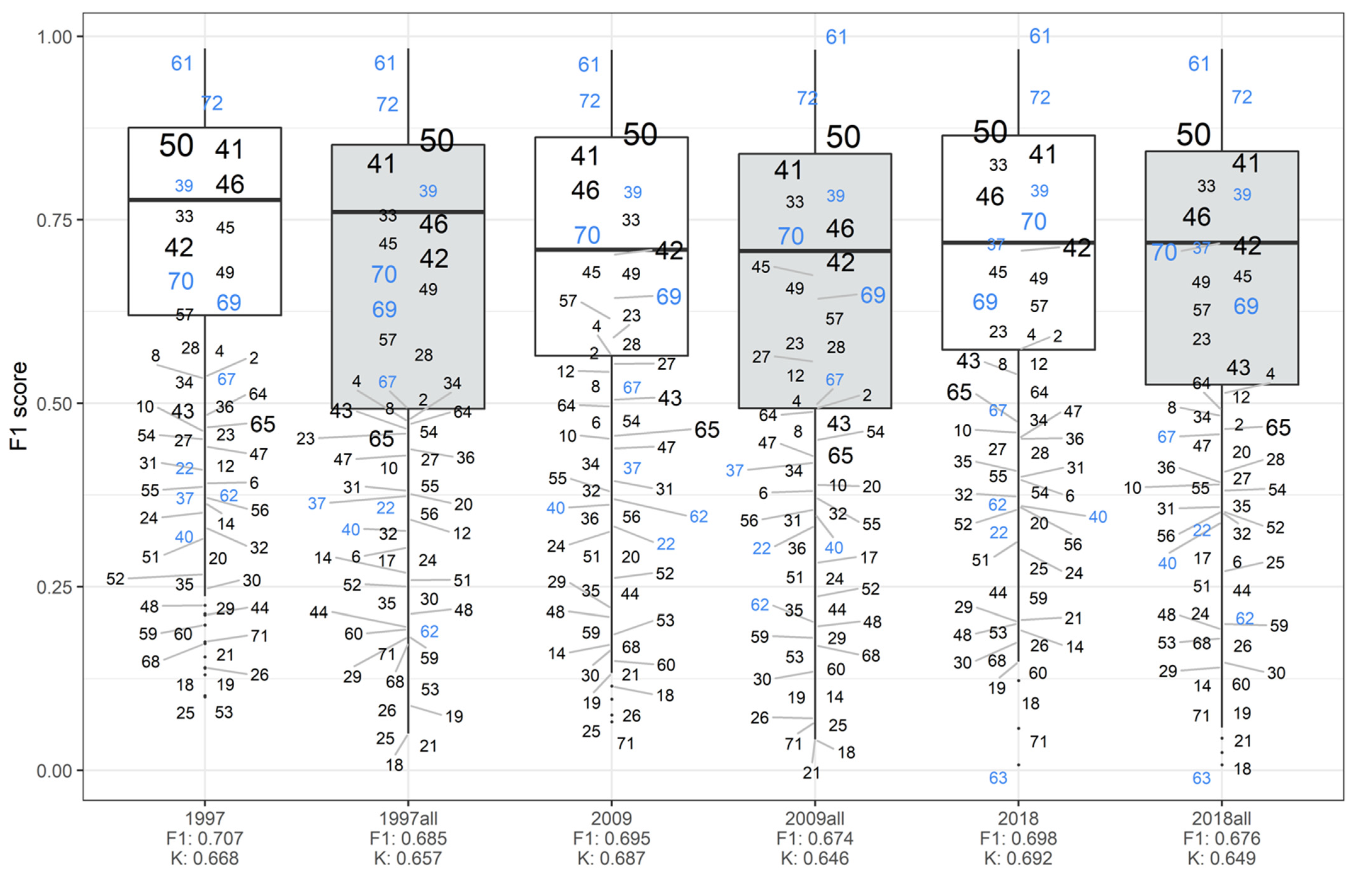
  104. Grandini, M.; Bagli, E.; Visani, G. Metrics for Multi-Class Classification: An Overview. arXiv 2020, arXiv:2008.05756. [Google Scholar]
  105. West, T.O.; Page, Y.L.; Huang, M.; Wolf, J.; Thomson, A.M. Downscaling Global Land Cover Projections from an Integrated Assessment Model for Use in Regional Analyses: Results and Evaluation for the US from 2005 to 2095. Environ. Res. Lett. 2014, 9, 64004. [Google Scholar] [CrossRef] [Green Version]
  106. Ivits, E.; Koch, B.; Blaschke, T.; Jochum, M.; Adler, P. Landscape Structure Assessment with Image Grey-values and Object-based Classification at Three Spatial Resolutions. Int. J. Remote Sens. 2005, 26, 2975–2993. [Google Scholar] [CrossRef]
  107. McGarigal, K.; Marks, B.J. FRAGSTATS: Spatial Pattern Analysis Program for Quantifying Landscape Structure; Gen. Tech. Rep. PNW-GTR-351; U.S. Department of Agriculture, Forest Service, Pacific Northwest Research Station: Portland, OR, USA, 1995; Volume 351, pp. 1–122. [CrossRef]
  108. Uuemaa, E.; Roosaare, J.; Mander, Ü. Scale Dependence of Landscape Metrics and Their Indicatory Value for Nutrient and Organic Matter Losses from Catchments. Ecol. Indic. 2005, 5, 350–369. [Google Scholar] [CrossRef]
  109. Riitters, K.H. Downscaling Indicators of Forest Habitat Structure from National Assessments. Ecol. Indic. 2005, 5, 273–279. [Google Scholar] [CrossRef]
  110. Levins, R. The strategy of model building in population biology. Am. Sci. 1966, 54, 421–431. [Google Scholar]
  111. Rockstrom, J.; Steffen, W.; Noone, K.; Persson, A.; Chapin, F.S.; Lambin, E.F.; Lenton, T.M.; Scheffer, M.; Folke, C.; Schellnhuber, H.J.; et al. A Safe Operating Space for Humanity. Nature 2009, 461, 472–475. [Google Scholar] [CrossRef]
  112. Wulder, M.A.; Masek, J.G.; Cohen, W.B.; Loveland, T.R.; Woodcock, C.E. Opening the Archive: How Free Data Has Enabled the Science and Monitoring Promise of Landsat. Remote Sens. Environ. 2012, 122, 2–10. [Google Scholar] [CrossRef]
  113. Zhu, Z.; Woodcock, C.E. Continuous Change Detection and Classification of Land Cover Using All Available Landsat Data. Remote Sens. Environ. 2014, 144, 152–171. [Google Scholar] [CrossRef] [Green Version]
  114. Brown, D.G.; Walker, R.; Manson, S.; Seto, K. Modeling Land Use and Land Cover Change. In Land Change Science; Remote Sensing and Digital Image Processing; Springer: Dordrecht, The Netherlands, 2012; pp. 395–409. ISBN 978-94-007-4306-9. [Google Scholar]
  115. Giuliani, G.; Dao, H.; De Bono, A.; Chatenoux, B.; Allenbach, K.; De Laborie, P.; Rodila, D.; Alexandris, N.; Peduzzi, P. Live Monitoring of Earth Surface (LiMES): A Framework for Monitoring Environmental Changes from Earth Observations. Remote Sens. Environ. 2017, 202, 222–233. [Google Scholar] [CrossRef]
  116. Purss, M.B.J.; Lewis, A.; Oliver, S.; Ip, A.; Sixsmith, J.; Evans, B.; Edberg, R.; Frankish, G.; Hurst, L.; Chan, T. Unlocking the Australian landsat archive—From dark data to high performance data infrastructures. GeoResJ 2015, 6, 135–140. [Google Scholar] [CrossRef] [Green Version]
  117. Ryan, B. The Benefits from Open Data Are Immense. Geospat. World 2016, 10, 72–73. [Google Scholar]
  118. Pasquarella, V.J.; Holden, C.E.; Kaufman, L.; Woodcock, C.E. From imagery to ecology: Leveraging Time series of all available landsat observations to map and monitor ecosystem state and dynamics. Remote Sens. Ecol. Conserv. 2016, 2, 152–170. [Google Scholar] [CrossRef]
  119. Hermosilla, T.; Wulder, M.A.; White, J.C.; Coops, N.C.; Hobart, G.W.; Campbell, L.B. Mass Data Processing of Time Series Landsat Imagery: Pixels to Data Products for Forest Monitoring. Int. J. Digit. Earth 2016, 9, 1035–1054. [Google Scholar] [CrossRef] [Green Version]
  120. Inglada, J.; Arias, M.; Vincent, A.; Tardy, B.D.M.; Michel, J. Large Scale Automatic Land Cover Map Production with Sentinel-2 Image Time Series: Current Status and Outlooks. 2016. Available online: https://www.jordiinglada.net/stok/LivingPlanet/LandCoverSlides.pdf (accessed on 22 February 2022).
  121. Zioti, F.; Ferreira, K.R.; Queiroz, G.R.; Neves, A.K.; Carlos, F.M.; Souza, F.C.; Santos, L.A.; Simoes, R.E.O. A Platform for Land Use and Land Cover Data Integration and Trajectory Analysis. Int. J. Appl. Earth Obs. Geoinf. 2022, 106, 102655. [Google Scholar] [CrossRef]
  122. Han, H.; Yang, C.; Song, J. Scenario Simulation and the Prediction of Land Use and Land Cover Change in Beijing, China. Sustainability 2015, 7, 4260–4279. [Google Scholar] [CrossRef] [Green Version]
  123. Verburg, P.H.; Dearing, J.A.; Dyke, J.G.; van der Leeuw, S.; Seitzinger, S.; Steffen, W.; Syvitski, J. Methods and Approaches to Modelling the Anthropocene. Glob. Environ. Chang.-Hum. Policy Dimens. 2016, 39, 328–340. [Google Scholar] [CrossRef] [Green Version]
  124. Killough, B. CEOS Land Surface Imaging Analysis Ready Data (ARD) Description Document; CEOS: London, UK, 2016. [Google Scholar]
  125. Strobl, P.; Baumann, P.; Lewis, A.; Szantoi, Z.; Killough, B.; Purss, M.; Craglia, M.; Nativi, S.; Held, A.; Dhu, T. The Six Faces of the Data Cube. In Proceedings of the 2017 Conference on Big Data from Space, Toulouse, France, 28 November 2017; pp. 32–35. [Google Scholar]
  126. Chatenoux, B.; Richard, J.-P.; Small, D.; Roeoesli, C.; Wingate, V.; Poussin, C.; Rodila, D.; Peduzzi, P.; Steinmeier, C.; Ginzler, C.; et al. The Swiss Data Cube, Analysis Ready Data Archive Using Earth Observations of Switzerland. Sci. Data 2021, 8, 295. [Google Scholar] [CrossRef]
  127. Giuliani, G.; Chatenoux, B.; Bono, A.D.; Rodila, D.; Richard, J.-P.; Allenbach, K.; Dao, H.; Peduzzi, P. Building an Earth Observations Data Cube: Lessons Learned from the Swiss Data Cube (SDC) on Generating Analysis Ready Data (ARD). Big Earth Data 2017, 1, 100–117. [Google Scholar] [CrossRef] [Green Version]
  128. Gómez, C.; White, J.C.; Wulder, M.A. Optical Remotely Sensed Time Series Data for Land Cover Classification: A Review. ISPRS J. Photogramm. Remote Sens. 2016, 116, 55–72. [Google Scholar] [CrossRef] [Green Version]
Figure 1. Original LU/LC statistics with 72 classes (Arealstatistik) at a 100 m resolution from the 2013–2018 period.
Land 11 00615 g001
Figure 2. LC information with 29 classes from the National Base Map swissTLM3D for 2021.
Land 11 00615 g002
Figure 3. Downscaling land use statistics (2013–2018) in the area of Zermatt from 100 m to 25 m resolution using inverse distance weighting, expert knowledge, national base map, transport and river information at 25 m. (a) Expert system (details in Figure 4), (b) 1:25,000 base map, (c,c′) hectare land use information, (d,d′) downscaled land use, (e) 1:25,000 linear features (rivers, roads and rails), (f,f′) overlay of linear features to downscaled land use at 25 m resolution. Downscaling process (p1) and linear features addition (p2).
Land 11 00615 g003
Figure 4. Expert system showing the possible authorized Landuse100 categories within BaseMap25 units; (1) represents possible choices, (2) unique choice, and (3) the default choice in case of lack of decision. Ten land use categories remain unmatched (shaded). Three categories correspond to punctual or linear features (dark grey), and seven categories (light grey) correspond to different types of buildings that were merged with their surroundings (green). A full version of the expert table is available in the Supplementary Material Table S1.
Land 11 00615 g004
Figure 5. Land use downscaling at 25 m of Switzerland for the 2013–2018 period. Swiss regional parks boundaries in red. (See Figure 6 for legend interpretation.)
Land 11 00615 g005
Figure 6. Land use downscaling from 100 m to 25 m and overlay of linear features for state of Geneva for the three periods.
Land 11 00615 g006
Figure 7. Weighted boxplots showing the F1-scores from the 72 downscaled classes (Landuse25) compared to the original classes (Landuse100), for each period, with (“all”) and without linear features. Numbers along the boxplots represent the land use categories and their size the proportion of each category in the dataset. Blue represents categories attributed based on “swisstopo” original classes; black represents categories attributed based on IDW of the 36 nearest neighbors. Values under each boxplot are overall weighted mean F1-score (F1) and kappa coefficient (k) for the considered year and dataset.
Land 11 00615 g007
Figure 8. Percentage of all misclassifications for the 17 main classes of the 2018 downscaled LU without linear features. Legend lists categories that were misattributed.
Land 11 00615 g008
Figure 9. Absolute surface area difference from the downscaled map (Landuse25) categories compared to the original Landuse100 map.
Land 11 00615 g009
Figure 10. Comparison of the 1997 and 2018 LU/LC data with original 100 m resolution (above) and the downscaled outputs at 25 m (below) for the Bulle and Freiburg cities. Urban expansion (as well as other land cover changes and the smoothing effect) of this economically active region can be more easily visualized with the improved spatial resolution.
Land 11 00615 g010
Table 1. Data input sources.
InputNameResolutionProviderURL
Land Use Statistics
(1992/97, 2004/09, 2013/18)
Arealstatistik100 mSwiss Federal Statistical Officewww.bfs.admin.ch/bfs/en/home/services/geostat/swiss-federal-statistics-geodata/land-use-cover-suitability.html (accessed on 10 December 2021).
National Base Map
(2003, 2008)
Vector 2525 mswisstopowww.swisstopo.admin.ch/en/geodata/maps/smv/smv25.html (accessed on 10 December 2021).
National Base Map
(2021)
swissTLM3D25 mswisstopowww.swisstopo.admin.ch/en/geodata/landscape/tlm3d.html (accessed on 10 December 2021).
Publisher’s Note: MDPI stays neutral with regard to jurisdictional claims in published maps and institutional affiliations.

