Abstract
Agricultural land abandonment is a complex, multidimensional, and nonlinear global phenomenon driven by multiple factors and has contrasting impacts on agrobiodiversity, the environment, and society. Appropriate management strategies on abandoned cultivated land are helpful in maintaining food and ecological security. However, there are few studies on the management of cultivated land abandonment from the perspective of stakeholders. Based on the stakeholder perspective and focusing on the two main modes of farmland abandonment management, namely, “transfer-oriented management” and “condition-improved management”, this study constructs two evolutionary game models to analyze the interest conflicts, decision-making behaviors and interest game foci of different subjects in the two management modes. Simulation analysis is conducted to verify the equilibrium results of the evolutionary game to find the key problems in abandonment management and put forward corresponding management policies. This study reveals the internal mechanism of abandonment management, thus providing a theoretical basis for the classified management of abandoned cultivated land.
1. Introduction
Since the mid-twentieth century, with urbanization of rural populations in advanced and emerging industrial countries in the Americas and Europe, due to the continuous decline in agricultural comparative income and the accelerated transfer of the agricultural labor force to non-agricultural industries [1,2], large areas of farmland have been abandoned and gradually evolved into a global land use phenomenon [3]. For instance, between 1980 and 2000, the Spanish Region of Murcia saw more than 9% of its land abandoned, particularly soils with marginal agricultural productivity [4,5]. In just five years, from 2000 to 2015, China’s cultivated land area decreased by 1.44 million hm2 [5,6]. Risk areas for land abandonment are widespread in EU countries and are not limited to mountain regions [7].
The experience of developed countries also shows that cultivated land abandonment is a common phenomenon in the process of urbanization and industrialization. The global trend of abandonment is also strong. Despite the increasing global demand for agricultural products and the increasing scarcity of land suitable for farmland expansion [8], socioeconomic impacts, trade, institutional structure, land use policies, etc. [9,10], cultivated land abandonment is still a common land use change process in many countries and regions of the world. Characterized by a wide area, large quantity, and long duration [11,12], abandonment exists in Europe, the Mediterranean, Latin America, Africa, and Asia, to varying degrees.
Land abandonment has had a series of impacts on social economies and on the ecological environment, such as threatening agricultural economic development and food security, destroying farmland biodiversity and agricultural landscape heterogeneity [13], soil erosion [14], etc. The significant reduction in the crop sowing area directly caused by abandonment will lead to varying degrees of food production reduction and regional food shortages, which will then affect the goods and services provided by agricultural land, thus exerting a profound impact on society as a whole [15].
To mitigate these negative effects, appropriate management and conservation strategies are necessary [16]. Governments of various countries have taken a series of measures to curb the trend of abandonment [17], such as the “Common Agricultural Policy” in the European Union [18]. Europe also promulgated the LFA (less-favoured areas) [19] agricultural development policy, which aims to improve agricultural production efficiency by strengthening infrastructure construction to encourage and guide farmers to recultivate abandoned land, with financial support. To control land abandonment in mountainous and semi-mountainous areas, Japan introduced a direct-subsidy agricultural policy for mountainous and semi-mountainous areas in 2000, aiming to maintain agroforestry development in these areas with financial support [20].
At the same time, cultivated land abandonment has gradually become a research hotspot. Scholars have studied abandonment from various perspectives, such as economy, geography, ecology, humanity, and law. The research scope has expanded from the impacts of abandonment to the exploration of its driving factors, then to the observation, simulation, and prediction of the spatial and temporal distribution of abandonment. However, studies on the management of cultivated land abandonment are still scarce. Studies have asserted that some portion of the abandoned lands should be managed to address global issues, such as food insecurity and the need for biofuel [21,22].
Abandonment management is a complex behavioral game process involving stakeholders, including farmers, agricultural enterprises, and governments, with varied interest demands, interest expressions, and interest conflicts. Therefore, from the perspective of stakeholders, this paper uses an evolutionary game to study the management of cultivated land abandonment and carries out simulation analysis based on land abandonment in China. Through coordinating the interest relationships among various subjects, this paper helps in optimizing the management strategy of farmland abandonment and provides a reference for other countries and regions in the world. It also facilitates the formation of sustainable comprehensive agricultural production capacity and food security [23].
2. Literature Review
Evolutionary game theory (EGT) originates from the imitation dynamics proposed by Abrams (2006) [24] and Taylor and Jonker (1978) [25]. The difference between EGT and traditional game theory is that traditional game theory is based on the complete rationality of humans. However, in actual economic activities, perfectly rational participants are almost nonexistent. Veblen was the founder of the school of institutional economics [26]. He was the first to propose a critique of neoclassicism’s view that rationality encompasses the complex customary activities of humans. Thereafter, Arrow proposed the concept of limited rationality [27]. Simon provided the definition of the finiteness assumption for the first time [28].
EGT is a new research approach based on traditional game theory. Unlike traditional game theory, EGT assumes that human rationality is limited and that complete information conditions are unnecessary. Initially, EGT was commonly used in biological fields [29,30]. With the development of the internet and artificial intelligence (AI), EGT has been applied in many other fields. For instance, in the economics sphere, the EGT method is usually used to forecast future development trends [31,32]; in the medical field, EGT is used to analyze the voluntary vaccination method [33]; in the energy field, EGT is used to explore the behavioral strategies of private sectors from the perspectives of green energy generators and sellers [34]; in the field of pollution control, EGT is used to analyze the impact of the operational mechanisms of local governments’ different expenditure preferences on the production behavior of industrial polluting enterprises, to specify the behavioral characteristics and optimal strategies of local environmental management [35]. In addition, other disciplines have employed the EGT method to address forecasting or management problems [36,37].
Currently, EGT has been widely used in the study of cultivated land protection and management involving multiple stakeholders, including studies of land fallow [38], solutions to land hoarding and land inspector dilemmas [39,40], the conversion of arable land back to forests [41], the control of heavy metal pollution in cultivated land [42], farm land allocation [43,44], and land-use planning [45]. These studies show that the evolutionary game model can effectively clarify the contradictory foci of various stakeholders in land protection and the evolutionary characteristics of decision-making.
Abandonment management involves stakeholders, including farmers, agricultural enterprises, and governments. For different subjects, their different interest demands will affect the effectiveness of abandonment management policy. Farmers, agricultural enterprises, and local governments have a strong inclination to opportunism, and their goals are very different in the process of abandonment management. The application of EGT is helpful in establishing and improving the long-term supervision and incentive mechanisms, thus optimizing abandonment management strategy [46,47].
Although abandonment of productive cultivated land is a concern, few studies have explored the management strategies of abandoned cultivated land [48,49]. Joung et al. (2020) modeled two types of decision-making by farmers—individual decision-making for investing their efforts in rice cultivation to seek their own profits, and decision-making for investing their efforts in collective action, such as earthworks or irrigation works—to understand the decision-making of farmers who owned rice paddy fields that were being cultivated and to identify the conditions or institutions that would help the farmers in implementing an efficient management scheme [50]. That study adopted the EGT to investigate how to prevent farmers from abandoning the fields. That study was a pioneering attempt to apply EGT to abandoned land management. However, EGT is rarely applied to studies on cultivated land abandonment from the perspective of stakeholders.
The existing literature suggests that “transfer-oriented management” [51] and “condition-improved management” [52] are the two main management modes of land abandonment. In the first mode, for farmers who are unwilling or unable to engage in agriculture, policies are focused on perfecting the land transfer market to be specific and encouraging and guiding farmers to transfer land to scale farmer households or agricultural enterprises to curb land abandonment. In the second mode, for farmers who want to farm but need to abandon land due to poor agricultural production conditions, policies are focused on perfecting agricultural infrastructure construction and reducing production costs to increase agricultural income.
Based on the bounded rationality hypothesis and combining the two main modes of abandonment management, this paper discusses the interaction mechanism and evolutionary trend of each subject’s strategy choice under different parameters, thereby revealing the evolutionary characteristics of stakeholders’ decision-making behaviors in abandonment management and providing theoretical guidance for abandonment management.
3. Game Model I: Evolutionary Game and Simulation Analysis of Abandoned Land Transfer between Farmers and Agricultural Enterprises
3.1. Assumptions
In transfer-oriented management, when land transfer income exceeds farmers’ value expectations for land management rights, farmers will be willing to transfer cultivated land. The higher the transfer income, the better. However, agricultural enterprises1 pursue the acquisition of land management rights at minimum cost, so they will try to reduce the transaction costs of acquiring land management rights as much as possible. In the absence of supervision, conspiring with local governments has become a way for agricultural enterprises to achieve goals, but farmers’ interests are severely damaged at the same time. Therefore, to regulate the land transfer market, it is necessary for central governments to supervise the conspiracy between local governments and agricultural enterprises to ensure the protection of farmers’ interests. Specific assumptions are as follows.
- (1)
- Farmers and agricultural enterprises are game bodies with bounded rationality.
- (2)
- Agricultural enterprises intend to transfer into land and realize large-scale operations to maximize their interests. To simplify the model, situations in which agricultural enterprises do not transfer into land are not included in this study. There are two ways for agricultural enterprises to transfer into land: negotiated transfer and compulsory transfer. The first means transfering into farmers’ lands by negotiation; the second means transfering into farmers’ lands by conspiring with local government to force farmers to transfer land, for the purpose of obtaining more land at lower prices [53,54]. If the conspiracy of forced transfer is found by the central government, the agricultural enterprises would be punished at the cost (F), and farmers would receive a subsidy (B).
- (3)
- For farmers, in the case of transferring land, their land transfer incomes obtained by negotiated transfer and compulsory transfer are, respectively, and (); in the case of abandonment, the potential economic value of the abandoned land is denoted by owing to its potential production and social security functions. In addition, in the case of compulsory transfer, farmers need to pay costs (C) if they choose to keep abandoned cultivated land.
- (4)
- For agricultural enterprises, the transaction costs for negotiated transfers and compulsory transfers are and , respectively (). In the case of transferring land successfully, agricultural enterprises need to pay farmers land transfer incomes; otherwise, they do not need to do so. Agricultural enterprises’ operating incomes are and () in the cases of successful and unsuccessful land transfers, respectively.
- (5)
- Farmers’ strategy set is (transfer, abandonment). Assuming that farmers’ probability of transferring land is (), then their possibility of abandoning land is . Agricultural enterprises’ strategy set is (negotiated transfer, compulsory transfer). If the agricultural enterprise’s possibility of negotiated transfer is (), then its possibility of compulsory transfer is ().
3.2. Evolutionary Game Analysis
Based on the above assumptions, the following payment matrix is obtained (Table 1).

Table 1.
Payment matrix of the game between farmers and agricultural enterprises.
First, farmers’ incomes are calculated according to their different strategies. A farmer’s expected income from the land transfer strategy is as follows:
A farmer’s expected income by adopting the abandonment strategy is as follows:
Therefore, farmers’ average expected income is as follows:
The replication dynamic equation of farmers’ behavior strategies is further stated as follows:
Similarly, agricultural enterprises’ incomes are calculated according to their different strategies. An agricultural enterprise’s expected income by negotiated transfer is as follows:
An agricultural enterprise’s expected income by compulsory transfer is as follows:
Therefore, agricultural enterprises’ average expected income is as follows:
The replication dynamic equation of agricultural enterprises’ behavior strategy is further stated as follows:
The simultaneous replication dynamic equations of the behavior strategies of farmers and agricultural enterprises are as follows:
If , the equilibrium solutions (i.e., the local equilibrium points) of the dynamic system of the evolutionary game between farmers and agricultural enterprises are (), (), () and (),. Thus, the Jacobi matrix of the game system is obtained as follows:
Among the above matrices,
According to Friedman (1991), the local stability analysis of the Jacobi matrix can test the local equilibrium stability of population dynamics [55]. Therefore, the determinant det.J and trace tr.J corresponding to the Jacobi matrix J are calculated as follows:
If the above local equilibrium points are substituted into the simultaneous equations of det.J and tr.J, the signs of each local equilibrium point are calculated, and their stability is judged (Table 2).
Table 2.
Values of the determinant and trace of the Jacobi matrix of the game system between farmers and agricultural enterprises.
Table 2 shows that the trace of the Jacobi matrix corresponding to the central point () is 0, indicating that this point is not a stable equilibrium point, so we do not have to discuss it for the time being. It is known that , so the signs of the determinants and traces of each local equilibrium point in Table 2 can be judged by comparing farmers’ transfer incomes, , with abandonment incomes, .
- (1)
- When a farmer’s abandonment income, , exceeds the transfer income, , as shown in Table 3, the stability of the game system can be judged by scenario analysis.
Table 3. Results of local equilibrium stability of the game system between farmers and agricultural enterprises.
Table 3 shows that when , point () is the stable equilibrium point in any situation. That is, (abandonment, compulsory transfer) is the final stable equilibrium strategy combination of the evolutionary game. However, this combination fails to achieve the social goal of alleviating abandonment and promoting land transfer. In this case, if and are satisfied simultaneously, then point () becomes a stable equilibrium point of the game. That is, (transfer, negotiated transfer) is also a stable equilibrium strategy combination of the evolutionary game. This combination not only alleviates abandonment through land transfer but also ensures farmers’ interests, which accords with social expectations.
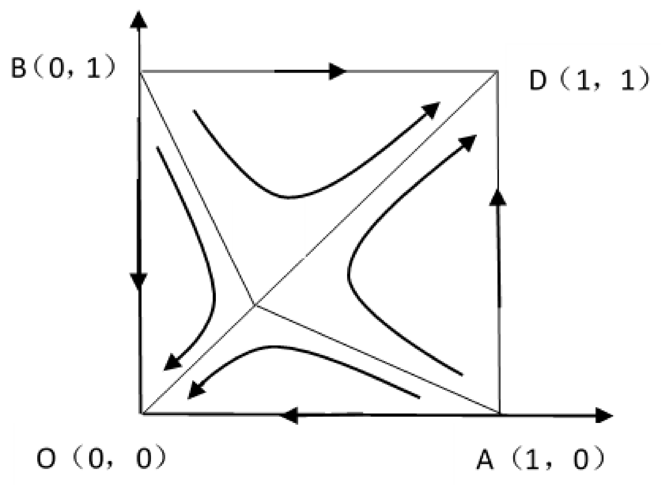
Figure 1 is the evolutionary phase diagram of the game under the conditions of and . Point E is the saddle point (). When the initial strategy combination of the game falls within the quadrilateral AEBD, the game system will eventually converge to D (). Specifically, (transfer, negotiated transfer) will become the final stable equilibrium strategy combination of the evolutionary game. The larger the area of the quadrilateral AEBD, the greater the probability that the game will converge to (). In contrast, when the initial strategy combination falls within the quadrilateral AEBO, the game system will eventually converge to O (). Specifically, (abandonment, compulsory transfer) will become the final stable equilibrium strategy combination of the evolutionary game. The larger the area of the quadrilateral AEBO, the greater the probability that the game will converge to (). To make the game system eventually converge to the stable equilibrium (transfer, negotiated transfer) expected by society along path ED, saddle point E should be closer to point O so that the area of the quadrilateral AEBD is expanded. According to Figure 1, , indicating that and are negatively linearly correlated. Therefore, the following measures can be taken to reduce the value of : improving the information transparency of the supply and demand parties in the land transfer market, introducing intermediaries in the land transfer market to reduce the transaction costs of negotiated transfers, aggravating penalties (F) for agricultural enterprises, and increasing farmers’ compensation (B) in cases of compulsory transfers.
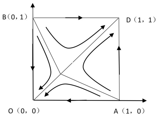
Figure 1.
Evolutionary phase diagram of the game between farmers and agricultural enterprises.
- (2)
- When a farmer’s transfer income, , exceeds abandonment income, , as shown in Table 4, the stability of the game system can be judged by scenario analysis.
Table 4. Results of the local equilibrium stability of the game system between farmers and local governments.
Scenario 1: and . Its economic significance is as follows: agricultural enterprises’ cost of a compulsory transfer exceeds that of a negotiated transfer, and a farmer’s transfer income is greater than the potential value of the abandoned land. In this case, the evolutionary game will converge to (); that is, (transfer, negotiated transfer) is the final equilibrium strategy combination of the evolutionary game, which is expected by society. To achieve this convergence, the following measures can be undertaken: aggravate the penalties (F) for agricultural enterprises in cases of compulsory transfer; take appropriate measures to reduce the transaction cost (); and increase farmers’ rent incomes () in the land transfers.
Scenario 2: . Regardless of the values of , the evolutionary game will converge to (). That is, (transfer, compulsory transfer) is the final equilibrium strategy combination of the evolutionary game. In this scenario, although farmers will receive certain compensation from interest redistribution by the central government, agricultural enterprises will still collude with the local government for maximized interests due to weak punishments. In this case, land transfers are unstable, and farmers may not abide by land transfer contracts. Therefore, transfer and compulsory transfer is not the most ideal game equilibrium strategy. The stable equilibrium strategy of the game can evolve to Scenario 1 when the punishment for agricultural enterprises in cases of compulsory transfer is aggravated.
Scenario 3: and . No stable equilibrium solution exists in this case.
In conclusion, when a farmer’s transfer income, , exceeds abandonment income, , two possible stable equilibrium strategies exist in the evolutionary game. If and , then the game converges to the strategy combination (transfer, negotiated transfer) expected by society. If , then the game converges to the strategy combination (transfer, compulsory transfer), but it is not optimal.
3.3. Simulation Analysis
To verify the results of the above evolutionary game and intuitively show the systematic evolution path, Python 3.7 was adopted to simulate the game. In the following analysis, the evolution of the game between farmers and agricultural enterprises under the constraints of a central government is simulated by assigning values to the parameters according to different scenarios.
- (1)
- According to the analysis in Section 3.2, when a farmer’s transfer income, , is less than the abandonment income, , if and , there may exist two stable equilibrium strategy combinations in the evolutionary game, and the final result of the evolutionary game is related to the position of central point E and the probability value of the initial strategy. Specifically, the closer central point E is to the upper right, the greater the probability that the evolutionary game will converge to (). In contrast, the closer the central point is to the lower left, the higher the probability of converging to (). Following are the simulations by parameter assignments in different situations.
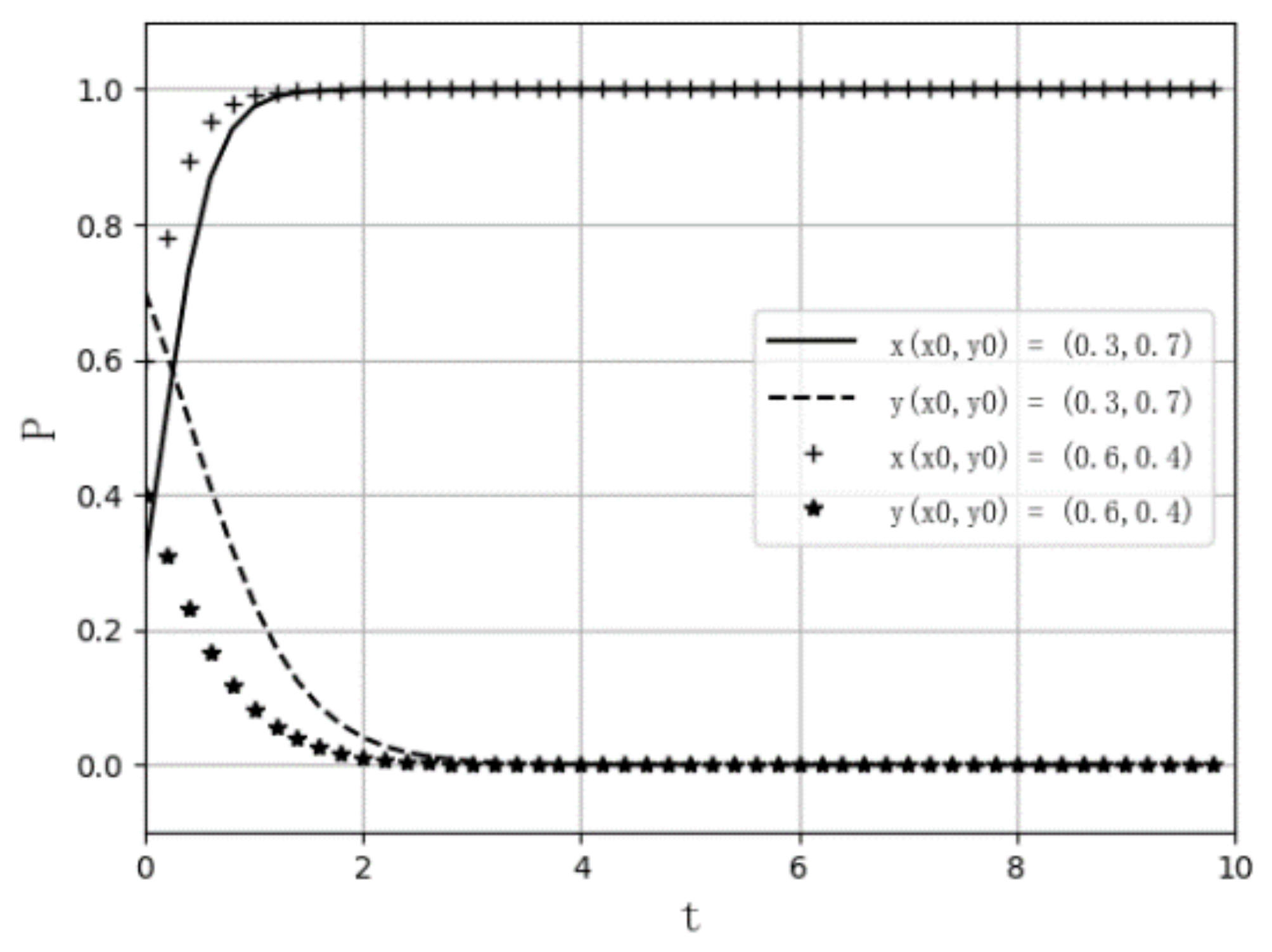
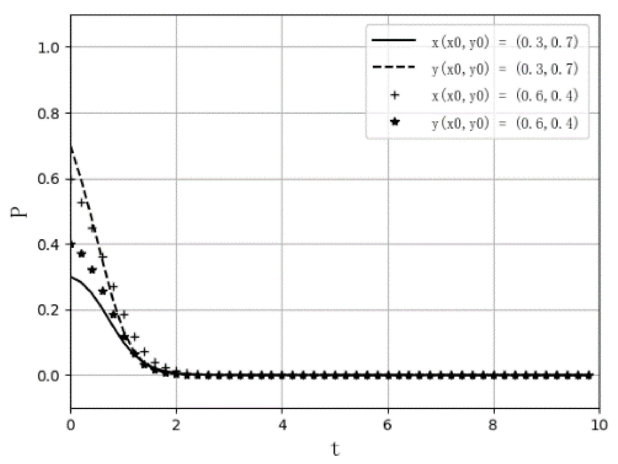
Set the parameter values as , , , , , , , , and set the initial values of () as () and (), respectively, so the center point E is (), and is located at the upper right of the evolutionary phase diagram. The simulation results are shown in Figure 2. At this moment, so long as the probability value of the initial strategy combination falls within the scope of the quadrilateral AEBO, no matter how the probability value changes, the game system will eventually converge to (). Specifically, (transfer, compulsory transfer) will become the stable equilibrium strategy of the evolutionary game, which is in accordance with the above analysis.

Figure 2.
Path diagram of the evolutionary game on abandoned land transfer between farmers and agricultural enterprises under constraint located at the upper right).
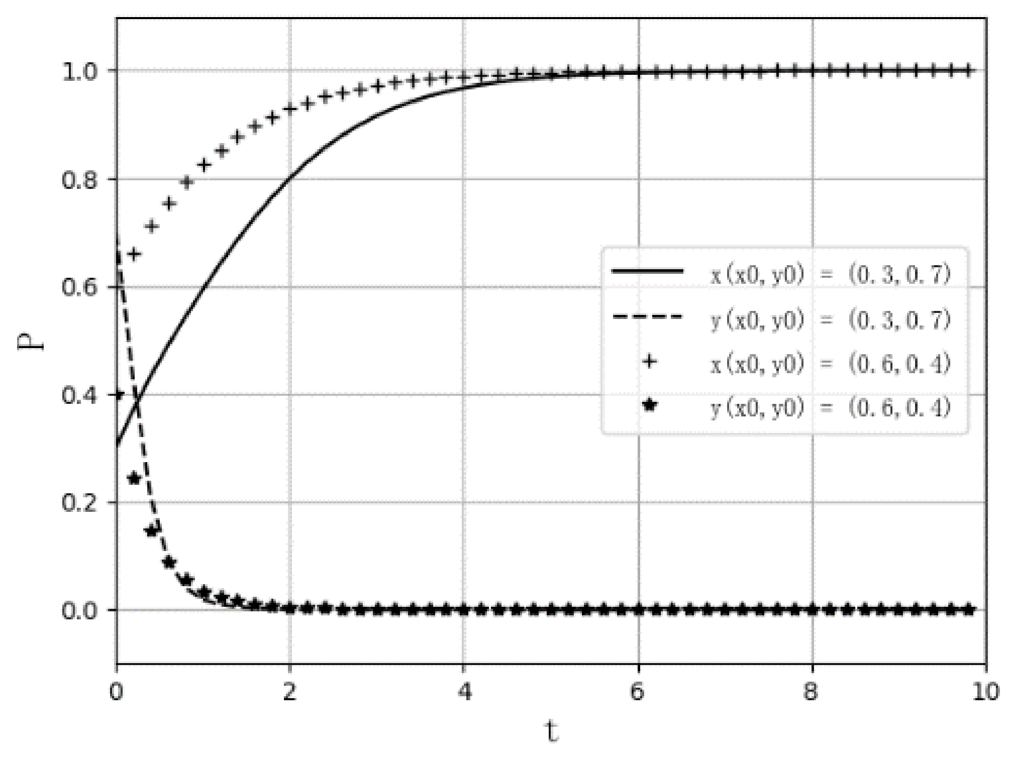
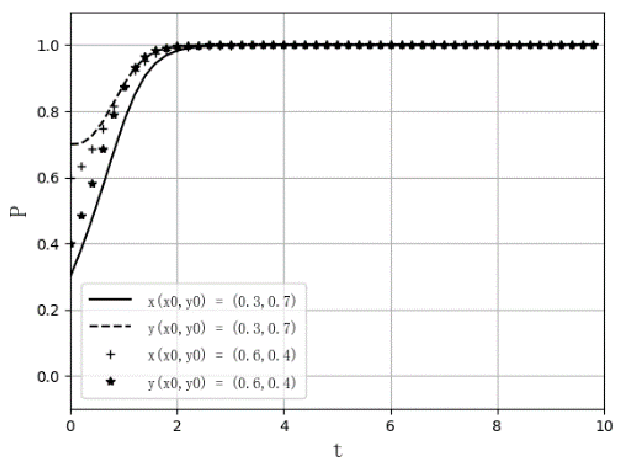
Set the parameter values as , , , , , , , , and set the initial values of () as () and (), respectively, so the center point E is (), and is located at the lower left of the evolutionary phase diagram. The simulation results are shown in Figure 3. At this moment, so long as the probability value of the initial strategy combination falls within the scope of the quadrilateral AEBD, no matter how the probability value changes, the game system will eventually converge to (). Specifically, (transfer, negotiated transfer) will become the stable equilibrium strategy of the evolutionary game, which is in accordance with the above analysis.

Figure 3.
Path diagram of the evolutionary game on abandoned land transfer between farmers and agricultural enterprises under constraints located at the lower left).
- (2)
- According to the analysis in Section 3.2, when a farmer’s transfer income, , exceeds abandonment income, , the game system will converge to different results with the change of and . The following are the simulations by parameter assignments in different situations.
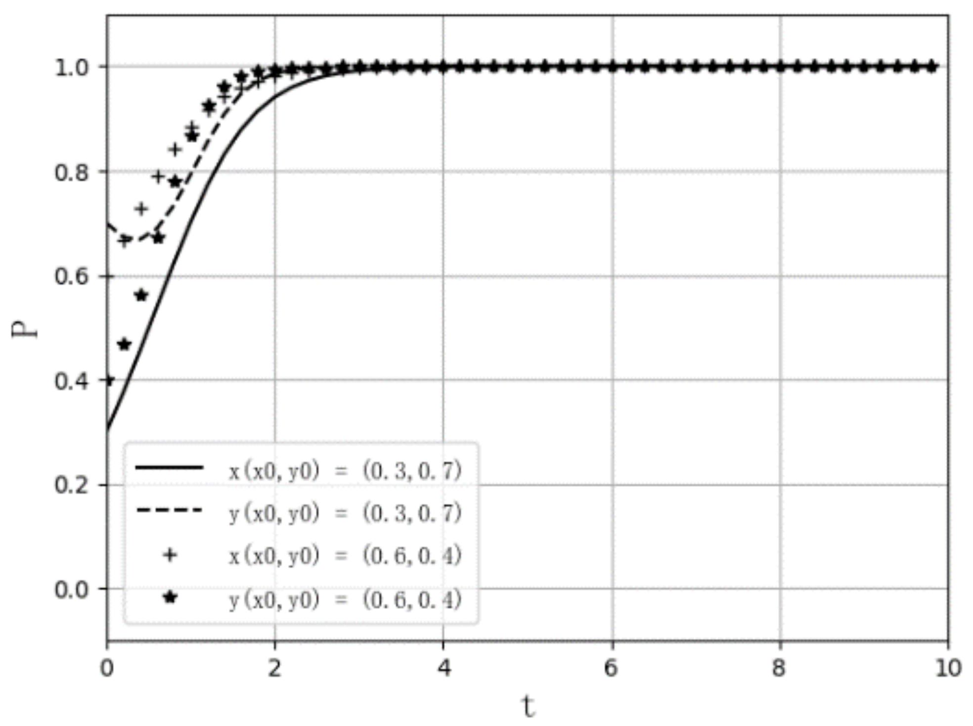
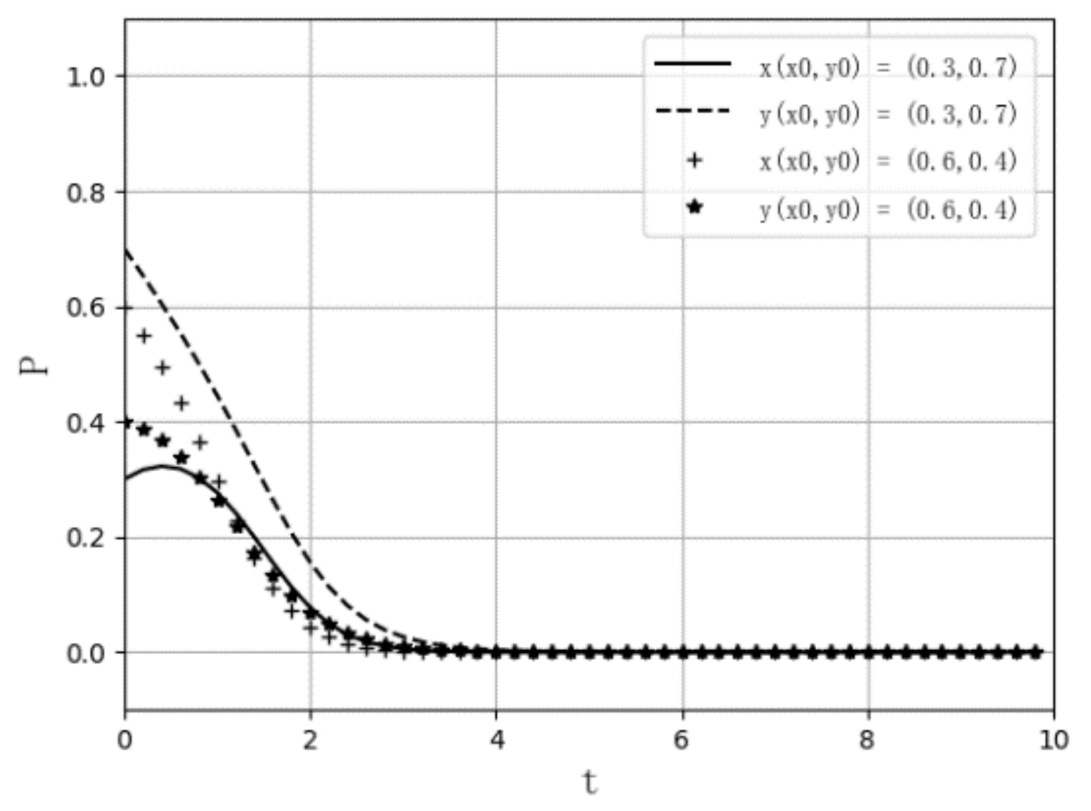
When and , set the parameter values as , , , , , , , , and set the initial values of () as () and (), respectively. The simulation results are shown in Figure 4. At this moment, no matter how the probability value of the initial strategy combination changes, the game system will eventually converge to (). Specifically, (transfer, negotiated transfer) will become the stable equilibrium strategy of the evolutionary game, which is in accordance with the above analysis.
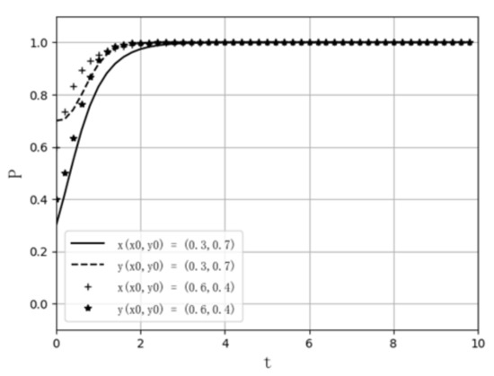
Figure 4.
Path diagram of the evolutionary game on abandoned land transfer between farmers and agricultural enterprises under constraints , ).
When , no matter what the values of and are, the game system will converge to (). is taken as an example to conduct simulation verification. Set the parameter values as , , , , , , , and , and set the initial values of as and , respectively. The simulation results are shown in Figure 5. In this case, no matter how the probability value of the initial strategy combination changes, the game system will eventually converge to (). Specifically, (transfer, compulsory transfer) will become the stable equilibrium strategy of the evolutionary game, which is in accordance with the above analysis.

Figure 5.
Path diagram of the evolutionary game on abandoned land transfer between farmers and agricultural enterprises under constraints ).
4. Game Model II: Evolutionary Game and Simulation Analysis of Abandoned Land Reclamation between Farmers and Local Government
4.1. Assumptions
In condition-improved management, farmers who are suitable for recultivation and local government have the motivation to maximize their own interests. For farmers, when their recultivation incomes exceed their non-agricultural incomes during abandonment, they will recultivate, or otherwise abandon the land. If a local government takes measures to improve the infrastructure construction or production conditions for agricultural production, the increase in agricultural income will enhance farmers’ willingness to recultivate. For local governments, when their political achievement in recultivation is greater than the cost invested in infrastructure improvement, the local government will obey the superior government’s requirement to promote recultivation, or otherwise take no action. However, farmers may still abandon land even though the infrastructure is improved by the local government. Therefore, local governments face uncertain risks, including poor political performance or even punishment by superior governments. According to the above analysis, the specific assumptions are as follows.
- (1)
- Local government and farmers are game bodies with bounded rationality.
- (2)
- A denotes the local government’s cost of agricultural infrastructure construction, G denotes its political achievement in promoting recultivation, and D denotes the punishment if it fails to promote recultivation.
- (3)
- Farmers will receive agricultural income I and subsidy B if the land is recultivated. However, if farmers continue to abandon land, they will lose the subsidy and receive punishment F. denotes a farmer’s non-agricultural income during abandonment. Owing to the old-age security function of cultivated land assets for Chinese farmers and its economic value [56], abandoned land still possesses a certain potential value, which is denoted by R.
- (4)
- In a game system, the benefits and costs of game bodies are mutually affected by their strategies, so it is essential to make assumptions about local government and farmers’ costs and benefits. First, in the case of implementing policies of the superior government, local governments will obtain political achievement , and farmers will obtain agricultural income . Second, in the case of violating policies of the superior government, if farmers recultivate land, the local government will obtain achievement, and farmers will obtain agricultural income, ; if farmers continue to abandon land, the local government will obtain no achievement or economic benefit, and farmers will obtain potential income .
- (5)
- Farmers’ strategy set is (recultivation, abandonment). Assuming that farmers’ probability of recultivation is (), then their possibility of abandoning land is . The local government’s strategy set is (implementation, violation). If the local government’s possibility of implementation is (), then its possibility of violation is (.
4.2. Evolutionary Game Analysis
Based on the above assumptions, the following payment matrix is obtained (Table 5).
Table 5.
Payment matrix of the game between farmers and local government.
First, a farmer’s income is calculated according to different strategies. A farmer’s expected income from the recultivation strategy is as follows:
A farmer’s expected income by adopting the abandonment strategy is as follows:
Therefore, farmers’ average expected income is as follows:
The replication dynamic equation of farmers’ behavior strategy is further stated as follows:
Similarly, we calculate the local government’s income according to its different strategies. The local government’s expected income from adopting the implementation strategy is as follows:
The local government’s expected income by adopting the violation strategy is as follows:
Therefore, the local government’s average expected income is as follows:
The replication dynamic equation of the local government’s behavior strategy is further obtained:
The simultaneous replication dynamic equations of the behavior strategies of farmers and local government are as follows:
If , the equilibrium solutions (i.e., the local equilibrium points) of the dynamic system of the evolutionary game between farmers and local government are (), (), (), () and ,, . Thus, the Jacobi matrix of the game system is obtained as follows:
Among the above matrices,
According to Friedman (1991), the determinant det.J and trace tr.J corresponding to the Jacobi matrix J are calculated as follows:
Substitute the above local equilibrium points into the simultaneous equations of det.J and tr.J. The signs of each local equilibrium point are calculated, and their stability is judged (Table 6).
Table 6.
Values of the determinant and trace of the Jacobi matrix of the game system between farmers and local government.
The local equilibrium point would be a stable equilibrium point of the evolutionary game if it satisfies det.J > 0 and tr.j < 0. Table 6 shows that the trace of the Jacobi matrix corresponding to the central point () is 0, indicating that this point is not a stable equilibrium point, so it is not essential to discuss it for the time being. Before judging the signs of det.J and tr.J corresponding to other local equilibrium points, we first need to compare the sizes of the parameters affecting the game system. According to the above hypothesis, , , . is the difference in a farmer’s agricultural income when the local government implements and violates the policy of investing in agricultural infrastructure construction. is the potential income difference of abandoned land when the local government implements and violates the policy of investing in agricultural infrastructure construction. Since the potential income of abandoned land depends on agricultural income, it can be inferred that the difference in agricultural income before and after agricultural infrastructure improvement exceeds that of the potential income of abandoned land; namely, . Based on this judgment, we discuss each equilibrium point by scenario analysis.
According to Table 7, this paper discusses the evolutionary process of the game in four scenarios.
Table 7.
Results of the local equilibrium stability of the game system between farmers and local government.
Scenario 1: and . Its economic implications are as follows: the local government violates the policy of the superior government, farmers’ recultivation incomes (agricultural income + subsidy) exceed the incomes from continuing abandonment (i.e., farm income + potential income from abandoning land less fines for policy violation), and the income difference between the local government’s implementation and violation strategies exceeds the cost of agricultural infrastructure investment. Table 7 shows that only the equilibrium point () is stable at this time; that is, (recultivation, implementation) is the stable equilibrium state of the game. This strategy combination helps in alleviating abandonment, realizing cultivated land value, and bringing positive benefits to local government. Therefore, this result is in line with the value orientation of the whole society.
The above scenario is influenced by , , , , , , , , etc. Among them, , , , , and are influenced by policy regulation. Therefore, to reach the equilibrium state, the following measures can be undertaken: regulating and perfecting the production and sales market to raise agricultural products’ value (), increasing agricultural subsidies (), enhancing the assessment of local governments’ achievements ( and ) on recultivation, and reducing the agricultural infrastructural investment () by technology introduction or innovation.
Scenario 2: . Its economic implications are as follows: the local government violates the policy of the superior government, farmers’ recultivation incomes exceed the potential incomes from abandonment, and the cost of agricultural infrastructure investment exceeds the income difference between the local government’s implementation and violation strategies. Table 7 shows that only the equilibrium point () is stable at this time; that is, (recultivation, violation) is the stable equilibrium state of the game. This may be due to the promoted value of agricultural products, increased agricultural subsidies, or constrained non-agricultural income due to high age. The reasons for the local government’s violation might be its lack of attention or the high investment cost of improving agricultural infrastructure. Although abandoned land is recultivated in this scenario, the equilibrium strategy is not optimal, and there still remains room for Pareto improvement. Effective measures can be taken to transform this equilibrium into the stable equilibrium of Scenario 1. For example, enhancing the assessment of the local government’s achievements in recultivation, reducing agricultural infrastructural investment by technology introduction or innovation, strengthening the local government’s sense of social responsibility, etc.
Scenario 3: and . Its economic implications are as follows: the local government violates the policy of the superior government, farmers’ incomes from abandonment exceed their recultivation incomes, and the income difference between the local government’s implementation and violation strategies exceeds the cost of agricultural infrastructure investment. Table 7 shows that the stable equilibrium point is (); that is, (abandonment, violation) is the stable equilibrium state of the game, and point () is unstable. However, as the signs of det.j and tr.j of the two local stable equilibrium points remain undetermined, further discussion is necessary.
According to Table 8, when , its economic implications are that the difference in farmers’ agricultural net incomes (i.e., farmers’ agricultural incomes less the potential income from abandoning land), between the local government’s implementation and violation strategies, exceeds the difference in farmers’ incomes between their recultivation and abandonment strategies when the local government violates the superior government’s policy. In this case, the stable equilibrium point of the game is (), that is, (recultivation, implementation) is the stable equilibrium state of the game. Consistent with Scenario 1, this state is in line with social expectations.
Table 8.
Stability results of the local equilibrium point in Scenario 3.
When , its economic implications are as follows: the difference in farmers’ incomes, between their recultivation and abandonment strategies when the local government violates the superior government’s policy, exceeds the difference in farmers’ agricultural net income (i.e., farmers’ agricultural income less the potential income from abandoning land) between the local government’s implementation and violation strategies. According to Table 8, neither () nor () are stable equilibrium points.
According to the above analysis, in Scenario 3, when , and , there are two stable equilibrium points () and () in the evolutionary game; specifically, both (abandonment, violation) and (recultivation, implementation) are stable equilibrium strategy combinations in the evolutionary game. However, (abandonment, violation) is not socially expected. Next, this section will analyze the process and probability of the game reaching the above two equilibrium points based on an evolutionary phase diagram (Figure 6), in which point E represents the central point ().
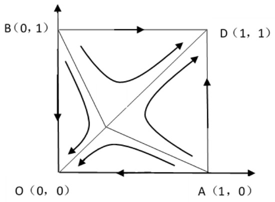
Figure 6.
Evolutionary phase diagram of the game between farmers and local government in Scenario 3.
When the initial strategy combination of the game falls within the quadrilateral AEBD, the game system will eventually converge to D (). Specifically, (recultivation, implementation) will become the final stable equilibrium strategy combination of the evolutionary game. The larger the area of quadrilateral AEBD, the greater the probability that the game will converge to (). In contrast, when the initial strategy combination falls within the quadrilateral AEBO, the game system will eventually converge to O (). Namely, (abandonment, violation) will become the final stable equilibrium strategy combination of the evolutionary game. The larger the area of quadrilateral AEBO, the greater the probability that the game will converge to (). To make the game system eventually converge to the stable equilibrium (recultivation, implementation) expected by society along path ED, saddle point E should be closer to point O so that the area of the quadrilateral AEBD is expanded. According to Figure 6, , indicating that and are negatively linearly correlated. Therefore, the following measures can be taken to reduce the value of : enhance the assessment of local governments’ achievements on recultivation, save agricultural infrastructure investment by technology introduction and improved management mode, increase agricultural subsidies appropriately, and increase agricultural income by perfecting agricultural infrastructure.
Scenario 4: and . Its economic implications are as follows: the local government violates the policy of the superior government, farmers’ incomes from abandonment exceed their recultivation incomes, and the cost of agricultural infrastructure investment exceeds the local government’s income difference between its implementation and violation strategies. Table 7 shows that the stable equilibrium point is (); that is, (abandonment, violation) is the stable equilibrium state of the game, and point () is unstable. However, as the signs of det.j and tr.j of the two local stable equilibrium points remain undetermined, further discussion is necessary.
According to Table 9, when , its economic implications are that the difference in farmers’ agricultural net incomes (i.e., farmers’ agricultural incomes less the potential income from abandoning land), between the local government’s implementation and violation strategies, exceeds the difference in farmers’ incomes between their recultivation and abandonment strategies when the local government violates the superior government’s policy. Neither () nor () are stable equilibrium points. When , its economic implications are as follows: the difference in farmers’ incomes, between their recultivation and abandonment strategies when the local government violates the superior government’s policy, exceeds the difference in farmers’ agricultural net incomes (i.e., farmers’ agricultural income less the potential income of abandoning land) between the local government’s implementation and violation strategies. Neither () nor () are stable equilibrium points.
Table 9.
Stability results of the local equilibrium point in Scenario 4.
In summary, in Scenario 4, when and , only one stable equilibrium point () exists. That is, (abandonment, violation) is the final stable equilibrium strategy combination of the evolutionary game. However, this combination fails to accord with social expectations.
4.3. Simulation Analysis
This paper adopted Python 3.7 to simulate the game. The evolutionary results of the game system wee verified by assigning values to the parameters in the above four scenarios.
- (1)
- Scenario 1: and . Set the parameter values as:, , , , , , , , , , and set the initial values of () as () and ().2 The simulation results are shown in Figure 7. This indicates that no matter how the probability value of the initial strategy combination changes, the game system will eventually converge to (). Specifically, (recultivation, implementation) will become the stable equilibrium strategy of the evolutionary game, which is in accordance with the above analysis.
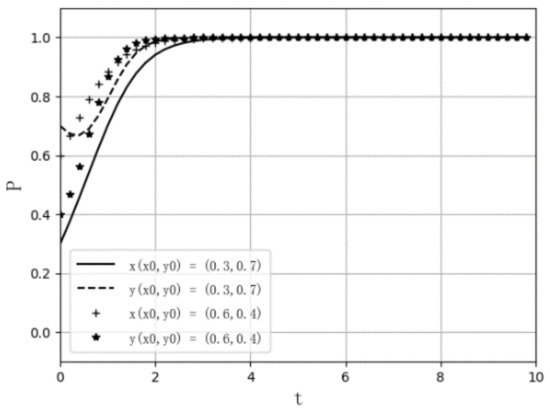 Figure 7. Path diagram of the evolutionary game of Scenario 1 ( and ).
 - (2)
- Scenario 2: and . Set the parameter values as:, , , , , , , , , , and set the initial values of () as (), (). The simulation results are shown in Figure 8. This analysis indicates that no matter how the probability value of the initial strategy combination changes, the game system will eventually converge to (). Specifically, (recultivation, violation) will become the stable equilibrium strategy of the evolutionary game, which is in accordance with the above analysis.
 Figure 8. Path diagram of the evolutionary game of Scenario 2 ( and ).
 - (3)
- Scenario 3:, and . There may exist two stable equilibrium strategy combinations in the evolutionary game, and the final result of the evolutionary game is related to the position of central point E and the probability value of the initial strategy. Specifically, the closer central point E is to the upper right, the greater the probability that the evolutionary game will converge to (). In contrast, the closer the central point to the lower left, the higher the probability of converging to (). Following is the simulation by parameter assignments in different situations.
Set the parameter values as , , , , , , , , , , and set the initial values of () as () and (), respectively, so center point E is (), and is located at the upper right of the evolutionary phase diagram. The simulation results are shown in Figure 9. At this moment, so long as the probability value of the initial strategy combination falls within the scope of quadrilateral AEBO, no matter how the probability value changes, the game system will eventually converge to (). Specifically, (abandonment, violation) will become the stable equilibrium strategy of the evolutionary game. This is in accordance with the above analysis.

Figure 9.
Path diagram of the evolutionary game of Scenario 3 (, and ).
Set the parameter values as , , , , , , , , , , and set the initial values of () as () and (), respectively, so center point E is (), and is located at the lower left of the evolutionary phase diagram. The simulation results are shown in Figure 10. At this moment, so long as the probability value of the initial strategy combination falls within the scope of the quadrilateral AEBD, no matter how the probability value changes, the game system will eventually converge to (). Specifically, (recultivation, implementation) will become the stable equilibrium strategy of the evolutionary game. This is in accordance with the above analysis.

Figure 10.
Path diagram of the evolutionary game of Scenario 3 (, and ).
- (4)
- Scenario 4: and . Set the parameter values as:, , , , , , , , , , and set the initial values of () as (), (). The simulation results are shown in Figure 11. This analysis indicates that no matter how the probability value of the initial strategy combination changes, the game system will eventually converge to (). Specifically, (abandonment, violation) will become the stable equilibrium strategy of the evolutionary game, which is in accordance with the above analysis.
 Figure 11. Path diagram of the evolutionary game of Scenario 4 ( and ).
5. Discussion and Conclusions
Focusing on the management of cultivated land abandonment, this study constructed an evolutionary game model to analyze the evolutionary process of farmers, agricultural enterprises, and local governments in the management process and explored the decision-making mechanisms of the interactions among various subjects. According to the game results, targeted policies were proposed to optimize abandonment management so that the game could converge to the ideal balance strategy combination expected by society.
In transfer-oriented management, the main game subjects were farmers, agricultural enterprises, and potential stakeholders (i.e., local governments). Without the supervision of a central government, agricultural enterprises would conspire with local governments to acquire land management rights through forced transfers. Farmers would transfer land only when their land transfer benefits were greater than the potential benefits of continued abandonment. Otherwise, farmers would continue to abandon farmland to obtain the potential benefits.
Under the supervision of a central government, the ideal stable equilibrium will appear only when a farmer’s transfer income is greater than the potential abandonment income, and agricultural enterprises’ cost of a forced transfer is greater than that of a negotiated transfer. However, other equilibrium solutions may also exist. To converge to the ideal equilibrium of the game system, it is essential to increase the transparency of land transfer supply and demand information, reduce the transaction cost of negotiated transfers by introducing the third-party intermediary in abandoned land transfers, increase agricultural enterprises’ punishment, and increase farmers’ compensation for forced transfer, etc.
In “condition-improved management”, the main game subjects were farmers and local governments. The evolution of the game included four scenarios, but only Scenario 1 and Scenario 3 reached the ideal game equilibrium. Scenario 1 indicated that when a local government violates the policies of a superior government, the overall income of farmers from resuming cultivation is greater than that from continuing with abandonment, and the difference between the total income obtained by the local government from implementing and violating the policies of the superior government is greater than the cost of agricultural infrastructure construction. At this point, the final equilibrium of the evolutionary game converges to the optimal equilibrium strategy combination expected by society (recultivation, implementation). Scenario 3 indicated that before a local government improves the agricultural infrastructure, farmers’ incomes from abandoning land are greater than those from recultivation. However, after improving the agricultural infrastructure, farmers’ incomes from recultivation would in turn exceed the incomes from abandonment, and the difference of local government’s total revenue under the two strategies would be greater than the cost of agricultural infrastructure construction. In this scenario, two equilibrium solutions exist. To converge to the ideal equilibrium of the game system, it is essential to strengthen the assessment of local governments in recultivation promotion, improve agricultural production conditions required by abandoned land to increase farmers’ farming incomes, save investment in agricultural production infrastructure construction by introducing advanced technology and management methods, and increase agricultural subsidies appropriately.
The stakeholders involved in abandonment management and their interest objectives, game focuses, and equilibrium strategies are universal and representative, and provide a reference for other regions of the world. The game and simulation results of the two management modes proposed in this study have been verified in practice. For example, the game result of “transfer-oriented management” has been verified in the abandonment management of Zhenyuan County, Qingyang City, Gansu Province, China, while “condition-improved management” has been verified in Chengmai County, Hainan Province, China. These two cases illustrated the theoretical guiding value of this study for abandonment management. However, the heterogeneity of the causes of cultivated land abandonment under different temporal and spatial conditions results in different stakeholders, conflicts of interest, and game focuses. For instance, the Chinese grassroots governments may have a great impact on cultivated land abandonment. Specifically, village collectives may act as an intermediary between farmers and agricultural enterprises in land transfers, while village collectives’ interests may conflict with those of farmers or agricultural enterprises. Therefore, evolutionary games among farmers, enterprises, and village collectives warrant further research. A game model of abandonment management involving different stakeholders can be built in the future based on this study, and the game model can be adjusted according to local conditions to expand the scope of this study’s applications.
Author Contributions
Q.C., H.X. and Q.Z. conceptualized the research and performed the validation; H.X. administered the project; Q.Z. developed the methodology, curated the data, conducted the formal analysis, and produced visualizations; Q.C. and Q.Z. wrote and prepared the original draft manuscript; Q.C. and H.X. reviewed and edited the manuscript; H.X. acquired funding; Q.Z. and Q.C. contributed to drafting the manuscript; Q.C. and H.X. approved the final version of the manuscript. All authors have read and agreed to the published version of the manuscript.
Funding
This study was supported by the National Natural Science Foundation of China (Nos. 41971243 and 41930757) and the Natural Science Foundation of Jiangxi Province (No. 20202ACB203004).
Institutional Review Board Statement
Not applicable.
Informed Consent Statement
Not applicable.
Data Availability Statement
Not applicable.
Acknowledgments
The authors would like to thank the reviewers and the editor, whose suggestions greatly improved the manuscript.
Conflicts of Interest
The authors declare no conflict of interest.
Notes
| 1 | In this study, agricultural enterprises refer to profitable economic organizations that obtain products through planting production and management. It mainly refers to large-scale agricultural operation subjects. The pursuit of agricultural enterprise is to obtain the land management right at the minimum cost, so it will reduce the transaction cost and consideration needed to obtain the right as much as possible. |
| 2 | Set different initial values for (x, y) to test if the initial values affect the results. |
References
- Romero-Calcerrada, R.; Perry, G.L. The role of land abandonment in landscape dynamics in the SPA ‘Encinares del rio Alberche y Cofio’, Central Spain, 1984–1999. Landsc. Urban Plan. 2004, 66, 217–232. [Google Scholar] [CrossRef]
- Meyfroidt, P.; Schierhorn, F.; Prishchepov, A.V.; Muller, D. Drivers, constraints and trade-offs associated with recultivating abandoned cropland in Russia, Ukraine and Kazakhstan. Glob. Environ. Chang. 2016, 37, 1–15. [Google Scholar] [CrossRef]
- Li, S.F.; Li, X.B. Global understanding of farmland abandonment: A review and prospects. J. Geogr. Sci. 2017, 27, 1123–1150. [Google Scholar] [CrossRef]
- Lasanta, T.; Arnáez, J.; Pascual, N.; Ruiz-Flaño, P.; Errea, M.P.; Lana-Renault, N. Space–Time process and drivers of land abandonment in Europe. Catena 2017, 149, 810–823. [Google Scholar] [CrossRef]
- Yao, Z.Y.; Zhang, L.J.; Tang, S.H.; Li, X.X.; Hao, T.T. The basic characteristics and spatial patterns of global cultivated land change since the 1980s. J. Geogr. Sci. 2017, 27, 771–785. [Google Scholar] [CrossRef] [Green Version]
- Cheng, W.M.; Gao, X.Y.; Ma, T.; Xu, X.L.; Chen, Y.J.; Zhou, C.H. Spatial-temporal distribution of cropland in China based on geomorphologic regionalization during 1990–2015. Acta Geogr. Sin. 2018, 73, 1613–1629. (In Chinese) [Google Scholar]
- Carolina, P.C.; Chris, J.C.; Vasco, D.; Carlo, L. Modelling agricultural land abandonment in a fine spatial resolution multi-level land-use model: An application for the EU. Environ. Model. Softw. 2021, 136, 104946. [Google Scholar]
- Cramer, V.A.; Hobbs, R.J.; Standish, R.J. What’s new about old fields? Land abandonment and ecosystem assembly. Trends Ecol. Evol. 2008, 23, 104–112. [Google Scholar] [CrossRef]
- Gellrich, M.; Baur, P.; Koch, B.; Zimmermann, N.E. Agricultural land abandonment and natural forest re-growth in the Swiss mountains: A spatially explicit economic analysis. Agric. Ecosyst. Environ. 2007, 118, 93–108. [Google Scholar] [CrossRef]
- Müller, D.; Kuemmerle, T.; Rusu, M.; Griffiths, P. Lost in transition: Determinants of post-socialist cropland abandonment in Romania. J. Land Use Sci. 2009, 4, 109–129. [Google Scholar] [CrossRef]
- Tan, S.K. Extent description and index system of sustainability judgment and its pattern of cultivated land abandoning. China Land Sci. 2003, 17, 3–8. (In Chinese) [Google Scholar]
- Chen, Q.R.; Xie, H.L. Mechanism of Farmers’ Cultivated Land Abandonment Behavior in Hilly and Mountainous Area—Based on the Theory of Planned Behavior; Economic Science Press: Beijing, China, 2020. (In Chinese) [Google Scholar]
- Song, W.; Zhang, Y. Farmland Abandonment Research Progress: Influencing Factors and Simulation Model. J. Resour. Ecol. 2019, 10, 345–352. [Google Scholar]
- Benayas, R.J.; Martins, A.; Nicolau, J.M.; Jennifer, J.S. Abandonment of agricultural land: An overview of drivers and consequences. CAB Rev. Perspect. Agric. Vet. Sci. Nutr. Nat. Resour. 2007, 2, 1–14. [Google Scholar]
- García-Ruiz, J.M.; Lana-Renault, N. Hydrological and erosive consequences of farmland abandonment in Europe, with special reference to the Mediterranean region—A review. Agric. Ecosyst. Environ. 2011, 140, 317–338. [Google Scholar] [CrossRef]
- Van Leeuwen, C.C.E.; Cammeraat, E.L.H.; de Vente, J.; Boix-Fayos, C. The evolution of soil conservation policies targeting land abandonment and soil erosion in Spain: A review. Land Use Policy 2019, 83, 174–186. [Google Scholar] [CrossRef]
- Chen, Q.R.; Xie, H.L. Research Progress and Discoveries Related to Cultivated Land Abandonment. J. Resour. Ecol. 2021, 12, 159–168. [Google Scholar]
- Pavel, M.; Vassil, V.; Anna, V.; Radko, R.; Vessela, S.; Zlatomir, D.; Nikola, V. Monitoring of the risk of farmland abandonment as an efficient tool to assess the environmental and socio-economic impact of the Common Agriculture Policy. Int. J. Appl. Earth Obs. Geoinf. 2014, 32, 218–227. [Google Scholar]
- Perrier-Cornet, P. The LFAs policies in France and the European Union. Primaff Rev. 2010, 36, 24–25. [Google Scholar]
- Hu, X. Investigation and analysis of agricultural direct subsidy policy in mountainous and semi-mountainous areas of Japan. Chin. Rural Econ. 2007, 6, 71–80. (In Chinese) [Google Scholar]
- Prishchepov, A.V.; Ponkina, E.V.; Sun, Z.; Bavorova, M.; Yekimovskaja, O.A. Revealing the intentions of farmers to recultivate abandoned farmland: A case study of the Buryat Republic in Russia. Land Use Policy 2021, 107, 105513. [Google Scholar] [CrossRef]
- Subedi, Y.R.; Kristiansen, P.; Cacho, O.; Ojha, R.B. Agricultural land abandonment in the Hill agro-ecological region of Nepal: Analysis of extent, drivers and impact of change. Environ. Manag. 2021, 67, 1–19. [Google Scholar] [CrossRef] [PubMed]
- Chen, Y.Q.; Li, X.B. Structural Change of Agricultural Land Use Intensity and Its Regional Disparity in China. Acta Geogr. Sin. 2009, 64, 469–478. (In Chinese) [Google Scholar] [CrossRef]
- Abrams, P.A. Rules for studying the evolutionary game. Evolution 2006, 60, 202–204. [Google Scholar] [CrossRef]
- Taylor, P.D.; Jonker, L.B. Evolutionary stable strategies and game dynamics. Math. Biosci. 1978, 40, 145–156. [Google Scholar] [CrossRef]
- Smith, J.M. Evolution and the theory of games. Q. Rev. Biol. 1976, 64, 41–45. [Google Scholar]
- Arrow, K. Social Choice and Personal Values; Willy: New York, NY, USA, 1951. [Google Scholar]
- Herbert, S. Administrative behavior. Am. J. Nurs. 1950, 50, 46–47. [Google Scholar]
- Fisher, R.A. The Genetic Theory of Natural Selection; Clarendon Press: Oxford, UK, 1930. [Google Scholar]
- Hamilton, W. Extraordinary sex rations. Science 1967, 156, 477–488. [Google Scholar] [CrossRef]
- Madeo, D.; Mazumdar, S.; Mocenni, C.; Zingone, R. Evolutionary game for task mapping in resource constrained heterogeneous environments. Future Gener. Comput. Syst. 2020, 108, 762–776. [Google Scholar] [CrossRef]
- Su, Z.F.; Yang, X.J.; Zhang, L.P. Evolutionary Game of the Civil-Military Integration With Financial Support. IEEE Access 2020, 8, 89510–89519. [Google Scholar] [CrossRef]
- Meng, X.Y.; Han, S.J.; Wu, L.L.; Si, S.B.; Cai, Z.Q. Analysis of epidemic vaccination strategies by node importance and evolutionary game on complex networks. Reliab. Eng. Syst. Saf. 2022, 219, 108256. [Google Scholar] [CrossRef]
- Liu, J.C.; Yu, J.; Yin, Y.; Wei, Q.S. An evolutionary game approach for private sectors’ behavioral strategies in China’s green energy public–private partnership projects. Energy Rep. 2021, 7, 696–715. [Google Scholar] [CrossRef]
- Fan, W.; Wang, S.; Gu, X.; Zhou, Z.Q.; Zhao, Y.; Huo, W.D. Evolutionary game analysis on industrial pollution control of local government in China. J. Environ. Manag. 2021, 298, 113499. [Google Scholar] [CrossRef] [PubMed]
- Wang, G.; Chao, Y.C.; Cao, Y.; Jiang, T.L.; Han, W.; Chen, Z.S. A comprehensive review of research works based on evolutionary game theory for sustainable energy development. Energy Rep. 2022, 8, 114–136. [Google Scholar] [CrossRef]
- Xie, H.L.; Jin, S.T. Evolutionary Game Analysis of Fallow Farmland Behaviors of Different Types of Farmers and Local Governments. Land Use Policy 2019, 88, 104122. [Google Scholar] [CrossRef]
- Xie, H.L.; Wang, W.; Zhang, X.M. Evolutionary Game and Simulation of Management Strategies of Fallow Cultivated land: A Case Study in Hunan Province, China. Land Use Policy 2018, 71, 86–97. [Google Scholar] [CrossRef]
- Zhang, X.L.; Bao, H.J.; Skitmore, M. The land hoarding and land inspector dilemma in China: An evolutionary game theoretic perspective. Habitat Int. 2015, 46, 187–195. [Google Scholar] [CrossRef]
- Wei, J.Z.; Liu, Y.P.; Zhang, F.; Jin, J.D. Game model of interest subject in ecological construction projects: A case study of government-led turning cultivated land back into forests and grasslands project. J. Desert Res. 2016, 36, 836–841. (In Chinese) [Google Scholar]
- Zhou, Z.F.; Liu, K.; Zeng, H.X. Multi-Evolutionary Game Study on Soil Heavy Metal Pollution Treatment. Ecol. Econ. 2021, 37, 183–193. (In Chinese) [Google Scholar]
- Xie, H.L.; Jin, S.T. Research on Arable Fallow Land Problems in Heavy Metal Contaminated Area from the Perspective of Interest Games. Ecol. Econ. 2018, 34, 190–195. (In Chinese) [Google Scholar]
- Mirja, M.; Jeroen, C.J.G.; Gundula, F.; Pablo, T. Land use decisions: By whom and to whose benefit? A serious game to uncover dynamics in farm land allocation at household level in Northern Ghana. Land Use Policy 2020, 91, 104325. [Google Scholar]
- Maleki, J.; Masoumi, Z.; Hakimpour, F.; Carlos, A.; Coello, C.A.C. A spatial land-use planning support system based on game theory. Land Use Policy 2020, 99, 105013. [Google Scholar] [CrossRef]
- Zhang, C.Q.; Chen, D.X.; Liang, L.X. Evolutionary games of the cultivated land protection between central government and local government. Commer. Res. 2016, 58, 151–157. (In Chinese) [Google Scholar] [CrossRef]
- Wu, X.L.; Liang, L.T.; Chen, C.Y. Behavior analysis of cultivated land protection subject and construction of compensation and incentive mechanism. Rev. Econ. Res. 2014, 71, 25–26. [Google Scholar] [CrossRef]
- Bierand, V.M.; Lin, S.M. Should the model for risk-informed regulation be game theory rather than decision theory? Risk Anal. 2013, 33, 281–291. [Google Scholar]
- Munroe, D.K.; van Berkel, D.B.; Verburg, P.H.; Olson, J.L. Alternative trajectories of land abandonment: Causes, consequences and research challenges. Curr. Opin. Environ. Sustain. 2013, 5, 471–476. [Google Scholar] [CrossRef]
- Joung, H.L.; Ryo, Y.; Hiroyuki, Y.; Mayuko, N. Preservation of the value of rice paddy fields: Investigating how to prevent farmers from abandoning the fields by means of evolutionary game theory. J. Theor. Biol. 2020, 495, 110247. [Google Scholar]
- Tan, Z.K.; Peng, Y.L. Investigation on the status quo of arable land abandonment and evasive measures in some counties and cities of Hubei province. Resour. Habitant Environ. 2003, 3, 37–39. (In Chinese) [Google Scholar]
- Yuba, R.S.; Paul, K.; Oscar, C. Drivers and consequences of agricultural land abandonment and its reutilisation pathways: A systematic review. Environ. Dev. 2021, 100681, In Press. [Google Scholar]
- Nathaniel, D.T. Viewpoint: How should policy respond to land abandonment in Europe? Land Use Policy 2021, 102, 105269. [Google Scholar]
- Lin, T.; Song, G. Evolutionary game analysis of farmland transfer strategy between stakeholders based on land-scale operation: Taking Keshan County as an example. J. Arid Land Resour. Environ. 2018, 32, 15–22. (In Chinese) [Google Scholar]
- Liu, H.Y. Study on Farmers’ income growth effect in rural land collective transfer—Taking the government-dominated agricultural land circulation mode as an example. Rural Econ. 2010, 7, 57–61. (In Chinese) [Google Scholar]
- Friedman, D. Evolutionary games in economics. Econometrica 1991, 59, 637–666. [Google Scholar] [CrossRef] [Green Version]
- Wang, Y.H.; Li, X.B.; Xin, L.J. Spatiotemporal evolution of the old-age security function of cultivated land assets for Chinese farmers in the past 30 years and its policy implications. Geogr. Res. 2020, 39, 956–969. [Google Scholar]


Publisher’s Note: MDPI stays neutral with regard to jurisdictional claims in published maps and institutional affiliations. |
© 2022 by the authors. Licensee MDPI, Basel, Switzerland. This article is an open access article distributed under the terms and conditions of the Creative Commons Attribution (CC BY) license (https://creativecommons.org/licenses/by/4.0/).