Deforestation in Continental Ecuador with a Focus on Protected Areas

Abstract

Forest conservation is of particular concern in tropical regions where a large refuge of biodiversity is still existing. These areas are threatened by deforestation, forest degradation and fragmentation. Especially, pressures of anthropogenic activities adjacent to these areas significantly influence conservation effectiveness. Ecuador was chosen as study area since it is a globally relevant center of forest ecosystems and biodiversity. We identified hotspots of deforestation on the national level of continental Ecuador between 1990 and 2018, analyzed the most significant drivers of deforestation on national and biome level (the Coast, the Andes, The Amazon) as well as inside protected areas in Ecuador by using multiple regression analysis. We separated the national system of protected areas (SNAP) into higher and lower protection levels. Besides SNAP, we also considered Biosphere Reserves (BRs) and Ramsar sites. In addition, we investigated the rates and spatial patterns of deforestation in protected areas and buffer zones (5 km and 10 km outwards the protected area boundaries) using landscape metrics. Between 1990 and 2018, approximately 4% of the accumulated deforestation occurred within the boundaries of SNAP, and up to 25.5% in buffer zones. The highest rates of deforestation have been found in the 5 km buffer zone around the protected areas with the highest protection level. Protected areas and their buffer zones with higher protection status were identified as the most deforested areas among SNAP. BRs had the highest deforestation rates among all protected areas but most of these areas just became BRs after the year 2000. The most important driver of deforestation is agriculture. Other relevant drivers differ between the biomes. The results suggest that the SNAP is generally effective to prevent deforestation within their protection boundaries. However, deforestation around protected areas can undermine conservation strategies to sustain biodiversity. Actions to address such dynamics and patterns of deforestation and forest fragmentation, and developing conservation strategies of their landscape context are urgently needed especially in the buffer zones of areas with the highest protection status.

1. Introduction

Forest ecosystems provide essential ecosystem services such as climate and water regulation, erosion prevention, carbon storage, timber, non-timber products, tourism and recreation [1,2,3]. For example, mountain forest catchments play an important role in runoff generation [4] and tropical rainforest influences the global carbon cycle [5,6]. About one-third of the global human population is directly dependent on forests and forest products as food, shelter, and income [5]. Forests also provide important habitat for flora and fauna. Approximately 80% of known amphibian species, 75% of all bird species and 68% of all mammal species have their habitat in forests [5,7]. However, many forest ecosystems are threatened by land use changes. Deforestation causes for example loss of species [8,9], carbon emissions and other greenhouse gases [10], soil erosion, and loss of organic matter [11]. In addition, climate variability causes diseases, climate stress for trees, and indirectly causes higher fire frequencies [12,13,14,15]. More than 20,000 tree species are on the International Union for Conservation of Nature (IUCN) Red List of Threatened Species [1,7,16]. Between 1990 and 2020, forests worldwide decreased from 32.5% to 30.8% of the total land area [5]. On average, 4,740,000 hectares of forest have been lost per year between 2010 and 2020. Highest forest losses occurred in South America and Africa (ibid.).

Forest ecosystems in South America are especially affected by high demand for timber, oil and minerals, food, and biomass [17,18,19]. Forest carbon loss between 2003 and 2016, for instance, was almost twice as large as carbon gains in the Amazon Basin [20] and soil organic matter on the surface was reduced by up to 60% in the Ecuadorian Amazon [21]. Furthermore, forest areas that are assigned to human land uses or strict protection cannot be clearly distinguished, especially in the Amazon Basin [22]. About 50% of the Amazon Basin is currently protected or indigenous territory but governmental concessions for mining and oil extraction overlap with about 24% of all official indigenous territories [20,23]. Indigenous people maintain forest as a source of their traditional livelihood and therefore contribute to nature conservation [24,25] and reducing forest loss [26,27]. In Ecuador for instance, government has allotted 48% of indigenous territories and protected areas (PAs) to oil mining companies, which hampers nature conservation [28].

Ecuador is a hotspot of global biodiversity and belongs to the top ten countries on the global level with the highest number of tree species [29]. However, Ecuador lost about 12% of its natural forest cover between 1990 and 2018 (ibid.). Forests in Ecuador are mainly affected by land use changes due to agricultural cultivation, pastures for livestock, urbanization, infrastructure, mining, and oil extraction [30,31]. The national system of protected areas (Sistema Nacional de Áreas Protegidas, SNAP) conserves biologically important areas and covers approx. 20% of the Ecuadorian land area [32]. Even though these areas are nationally protected, their buffer zones receive major anthropogenic pressure. Andrade-Núñez and Aide [33] analyzed nighttime light as an indicator of infrastructure and human activity inside and next to PAs in South America between 2001 and 2011. Ecuador and Venezuela had the highest infrastructural expansion in and around PAs, assuming pressure on PAs due to missing buffer zones and corridors. Currently, 22% of the forest ecosystems in Ecuador are threatened according to the IUCN Red List of Ecosystems [34]. Sierra et al. [35,36] and González-Jaramillo et al. [37] conducted spatial analyses of deforestation on national level. They identified the coastal biome as the most affected area of deforestation. Sierra et al. [35,36] suggested therefore the establishment of additional protected areas especially in the coastal biome and for dry ecosystems. Rivas et al. [38] is supporting this recommendation. They have focused on seasonal dry forest in the coastal biome and its protection levels. They showed that especially semi-deciduous forest represented highest fragmentation levels and need more effective protection. Currently existing PAs could partly prevent deforestation but would not be sufficient to conserve seasonal dry forests. Tapia-Armijos et al. [39] also analyzed seasonal dry forest but in addition montane evergreen forest, premontane evergreen forest, and shrubland. Besides continuous forest loss, they found more isolated and irregular forest patches and decreasing patch size in the Loja and Zamora Chinchipe Provinces in southern Ecuador since 1989, which could be related to better accessibility by new road constructions. Regarding the protection of forests in Ecuador, Van der Hoek [40] compared the effectiveness of PAs against deforestation by generalized linear models between 2000 and 2008. There were no differences between the age, size, and level of protection but he identified in general higher forest loss outside PAs. Our analysis reflects on multiple aspects of deforestation. More investigation is needed regarding the type(s) of pressure and the spatial patterns of deforestation in and around PAs on the national level of continental Ecuador. The analysis of causes and patterns of deforestation and forest fragmentation are important to monitor changes, to conclude for land use trends, to assess the effectiveness of the national protection status, to inform decision-making, and to counteract the negative impacts on biodiversity and human livelihood [34,35,41]. Geographical Information Systems (GIS) are of great support in detecting changes in the amount and distribution of forest, especially on a larger landscape scale and have been used in this study. This paper is guided by the following questions:

• Where are the accumulated areas of deforestation (hotspots) in Ecuador between 1990 and 2018?
• Which are the most significant driving forces of deforestation in Ecuador on national and biome level; and especially in protected areas?
• Which patterns of deforestation occur in and around protected areas? Do these patterns differ in buffer zones (5 km and 10 km buffer) and in protected areas of different protection status?
• Is the current protection system effective to maintain forest in protected areas?

2. Methods and Study Area

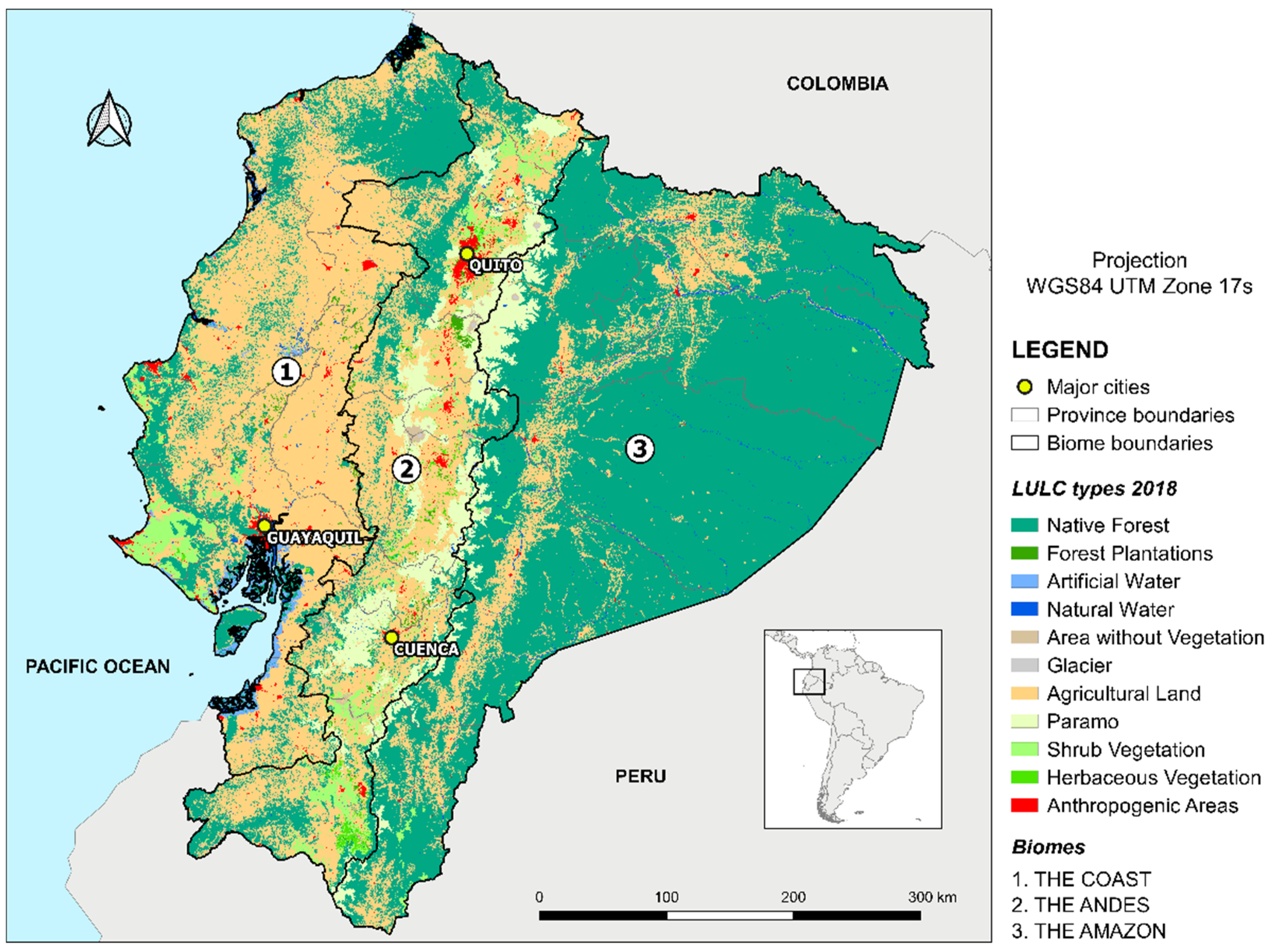
We started the analysis with the detection of hotspots of native forest losses on national level in Ecuador from 1990 to 2018 (method Section 2.4.1 and results Section 3.1) by using GIS. We analyzed changes in native forest cover according to the different IUCN equivalent categories (eq. cat.; Section 2.3) inside PAs, a 5 km buffer and 10 km buffer around PAs and identified fragmentation levels by using different landscape metrics (method Section 2.4.2 and results Section 3.2). Major drivers of deforestation were identified by multiple regression analyses (method Section 2.4.3 and results Section 3.3).

“Ecuador” in this study means continental Ecuador (without the Galapagos Islands). “Forest” indicates native forest. The land cover class “native forest” includes natural forest types such as cloud forest, dry forest, and manglar; excluding forest plantations [42]. Páramo as alpine highland shrubland is included in this analysis due to their ecological importance and the vulnerability caused by degradation and deforestation [43].

2.1. Ecuador

Ecuador is located in northwestern South America at the Pacific Ocean and demarcated by Peru and Colombia. The capital of Ecuador is Quito with approx. 1.6 million people and being with an altitude of 2850 m the second-highest capital city in the world. Continental Ecuador has three distinct biomes: The Coast, Andes and Amazon biome (Figure 1). The coastal biome is the lowland between the Pacific Ocean and the western part of the Andes. Soils are fertile due to sediments from rivers such as the Guayas that have transported fertile silts from the highlands to the floodplains. Its climate is influenced by the intertropical convergence zone and can therefore be impacted by the weather phenomenon, El Niño. The Andes biome covers the highest elevations within Ecuador and the western and eastern foothills of the Andes [44]. Many mountains are volcanoes. The Chimborazo volcano is the highest elevation in Ecuador with 6310 m. The eastern part of the Andes is transitioning to the rainforest of the Amazon basin. This area is influenced by the tropical air mass that often causes abundant rainfall (ibid.). Due to the high variation in biophysical and climatic conditions, Ecuador has a high variety of different ecosystems, e.g., rainforest, cloud forest, mangroves, and Páramo. Associated with the variety of ecosystems, Ecuador has a high biodiversity and many species are endemic [45,46].

Ecuador’s economy highly depends on mineral fuels and oil accounting with US $8.7 billion for about 39% of all exports. In addition, agriculture is the fourth most important economic sector for the country. It represents 9.63% of Ecuador’s GDP and 26.8% of employment by the economically active population [47]. The main uses of agricultural areas are pastures cultivated for livestock, permanent and transitory crops, e.g., banana, cocoa, coffee, sugar cane, corn, rice and potatoes [48]. Furthermore, 66.8% of the raw material used by the timber industry in 2014 came from forest plantations, 10.4% from native forests, 12.5% from pioneer formations, and 10.3% from agroforestry systems [49]. Ecuador’s main forest plantations are African palm, teak, melina, balsa, eucalyptus, pine, cedar and laurel [50].

2.2. Selection of Data

The basic data required for this study were collected from official national and international sources of continental Ecuador. Official national data were sourced from the Ministry of Environment, Water and Ecological Transition (MAATE; renamed in 2021; before, it was named as the Ministry of Environment of Ecuador—MAE) and the national Military Geographic Institute (IGM). These data included information about PAs, land use/land cover, and deforestation. International data were sources from, e.g., Open Street Map from Humanitarian Exchange Data.

Table 1. Basic data collected for the analysis of deforestation in continental Ecuador with a focus on protected areas. Data was provided by the Ministry of the Environment, Water and Ecological Transition (MAATE), the Energy and Non-Renewable Natural Resources Regulation and Control Agency (ARCERNNR), the Ministry of Tourism (MINTUR), and the Military Geographic Institute (IGM). International sources were Open Street Map from Humanitarian Exchange Data (HDX) and the Shuttle Radar Topography Mission (SRTM) from NASA (National Aeronautics and Space Administration).

Data	Format	Scale	Date of Reference	Source
Protected areas	Polygon shape file	1:250,000	2020	[51]
Deforestation from the periods 1990–2000, 2000–2008, 2008–2014, 2014–2016, and 2016–2018	Polygon shape files	1:100,000	1990–2018	[51]
Land Use/Land Cover	Polygon shape file	1:100,000	2018	[51]
Roads	Line shape file	-	2020	[52]
Rivers	Line shape file	1:250,000	2013	[53]
Lakes	Polygon shape file	1:250,000	2013	[53]
Mining concessions	Polygon shape file	-	2021	[54]
Touristic infrastructure	Point shape file	-	2002	[55]
Slope	Raster file	30 m	2000	[56]

indicates the characteristics of the data used. This data is the main input for the analysis of the landscape pattern, the estimation of the percentage of forest change over time, and the identification of main driving forces of deforestation in the country. For all data, the most updated available version was used.

2.3. Selection of Protected Areas Categories

The national system of protected areas in Ecuador (SNAP) has several protection categories [57]. The categories without or little human impact are national parks, wildlife refuges, ecological reserves, marine reserves, biological reserves, and geobotanical reserves. In contrast, Flora and Fauna Production Reserves and natural recreation areas allow human interventions. In order to follow international standards, we categorized the PAs of SNAP into the classes of IUCN (IUCN, 2021): Strict Nature Reserve Category (Category Ia), Wilderness Area (Category Ib), National Park (Category II), Natural Monument or Feature (Category III), Habitat/Species Management Area (Category IV), Protected Landscape/Seascape (Category V), and protected area with sustainable use of natural resources (Category VI). We followed the suggestion of MAATE [58] for the classification of SNAP to the IUCN equivalent. We further based our selection on PA descriptions in Boitani et al., Dudley, and Leroux et al. [59,60,61]. Higher protection status was assigned to national parks, and PAs that serve only for biodiversity and ecosystem protection. Highest protection status is assigned to Biological and Ecological Reserves (Reserva Ecologica and Reserva Biological). The aims of these protected areas are for biodiversity and ecosystem protection managed mainly by scientific research (IUCN cat. Ia/b) and directed management practices (IUCN cat. II-IV) in order to preserve the natural condition [58]. PAs with lower protection status were recreational areas and botanical gardens, among others (see

Table 2. Protection level classification of the Ecuadorian protected areas recognized by the national system of protected areas (SNAP = Sistema Nacional de Áreas Protegidas), according to [59,60,61]. The categories are equivalent to the International Union for Conservation of Nature (IUCN, [64]) and were based on MAATE [58]. Biosphere Reserves (BRs) and Ramsar sites (RAMs) were included in this list as Internationally Designated Areas (IDAs) and categorized as mixed protection. Number of areas ≥ 1 km², which is equivalent to 17.2% of the total number of areas (n = 2701) under this category. This table shows the selected protected areas for our analysis of landscape metrics that were established until 2018.

Protection Level	National and International Designations	Number of Areas	Internationally Recognized Equivalent Categories
High	Reserva Biologica	5	IUCN-Ia/b
	Reserva Ecologica	8	IUCN-Ia/b
	Parque Nacional	12	IUCN-II
	Reserva Geobotanica	1	IUCN-III
	Refugio de Vida Silvestre	10	IUCN-IV
Low	Área Nacional de Recreación	6	IUCN-V
	Área Ecologica de Conservacion	3	IUCN-VI
	Reserva de Producción de Flora y Fauna	3	IUCN-VI
Mixed	Biosphere Reserves	6	IDAs
	Ramsar Sites	18	IDAs

). These PAs are areas that offer a combination of protection and human land use, e.g., recreation and sustainable land management. In addition, there exist 6 internationally designated Biosphere Reserves (BR) and 18 Ramsar sites (RAMs) in Ecuador. BRs belong to the intergovernmental Man and the Biosphere Programme by UNESCO. BRs have a core zone (area of high protection level), a buffer zone and a transition area (development area). Their primary aim is the conservation of nature while allowing sustainable economic development. Local stakeholders can be involved in planning and management of the BR [62]. RAMs are internationally important wetland areas. The management of RAMs is guided by the corresponding international Convention [63]. BRs and RAMs were included in this list as Internationally Designated Areas (IDAs) and categorized as mixed protection status since high and low protection levels of PAs are overlapping inside these areas. Due to the overlapping areas, IDAs were analyzed separately from the IUCN equivalent categories. Other areas with effective area-based conservation measures such as the Socio Bosque Program were excluded because they are not legally protected areas. For our analysis of landscape metrics, only PAs were chosen that were established until 2018 (Table 2).

2.4. Analyses

2.4.1. Deforestation Hotspots

Deforestation hotspots were defined as areas that experience deforestation on more than 70% of the area in a 1 × 1 km² cell. We derived this information by overlaying a grid of 1 × 1 km² on the deforestation grid, showing the deforested areas detected between 1990 to 2018 in continental Ecuador. For each 1 × 1 km² cell, the proportion of deforested cells was calculated and classified as “low” (0 to 0.7) or “high” (>0.7 to 1).

2.4.2. Deforestation Rates and Patterns Inside Protected Areas and Buffer Zones

We assessed the effect of the protection status against deforestation by comparing deforestation occurrences inside PAs and the contiguous buffer areas in a 5 and 10 km buffer. The buffer distances were selected to maintain a similarity in the natural and environmental conditions for assessing the land cover change dynamics driven by anthropogenic activities (i.e., tourism, agriculture, and infrastructure) at local scale [65,66]. The information such as native forest cover, deforestation, and delineation of PAs was taken from MAATE (see Table 1). The total area of forest within buffer zones was quantified. The land cover classification of the year 1990 by MAATE was used as the baseline. Deforestation occurrences from year 2000, 2008, 2014, 2016, and 2018 were spatially intersected along buffer zones on forest cover range in order to quantify the amount of deforested area according to the range of buffer zone, year, and PA class. Overlapping buffer zones were merged together. Since BRs and RAMs are overlapping with nationally protected areas and in order to avoid double counting, we separated these in IDAs in our analysis from the analysis of PAs with IUCN equivalent categories.

In this study, the landscape metrics Number of Patches (NumP), Mean Patch Size (MPS), and Patch Size Coefficient of Variance (PSCoV) were calculated according to McGarigal and Marks [67]; NumP refers to the total number of forest patches in the landscape, MPS is a function of number of forest patches and total landscape area, and PSCoV measures relative variability about the mean. Using this metrics, we applied a fragmentation index (FI) proposed by the Andean Community of Nations [68] and previously used by MAATE [69] to measure the structure of forested ecosystems described as follows:

$$\mathit{FI}={{\displaystyle \sum }}_{i=1}^{n}E\prime ; \mathrm{with} i=\{\mathrm{NumP}, \mathrm{MPS}, \mathrm{PSCoV}\}$$

(1)

$$\frac{E-Emin}{Emax-Emin}=E^{\prime }$$

(2)

where, E_min equals the minimum value for variable E, E_max equals the maximum value for variable E, and E′ equals the normalized value of the variable E. For each zone (PAs, 5 km, and 10 km) landscape metrics NumP, MPS, and PSCoV where normalized and summed up to obtain an FI value ranging from 0 (low fragmentation) to 3 (high fragmentation). These values were averaged to provide an overview of the fragmentation index among the three zones, using the Jenks optimization method.

For assessing the effectiveness of PA establishment overall, we compared forest (loss) before and after PA establishment. We categorized the SNAP and IDAs into PAs established ≤1989, 1990–1999, 2000–2007, 2008–2013, 2014–2017, and ≥2018. For IDAs established ≤1989 and ≥2018 only one IDA was available, respectively.

2.4.3. Analysis of the Main Drivers of Deforestation

Identifying the drivers of deforestation is important to develop appropriate policy and measures to address the problems of ecosystem and biodiversity loss [8,70]. We analyzed selected direct drivers of deforestation according to Geist and Lambin [71]. Selection was based on availability of data. In this study, a multiple regression model was performed to determine the correlation of the direct drivers of deforestation on national and biome level. A multiple regression analysis is a statistical technique that allows to determine the correlations between more than two variables. Multiple regression models describe the response of a single variable Y that depends linearly on the behavior of several predictor variables X_n [72,73]. The multiple regression model is formulated as follows:

$$Y={\beta }_0+{\beta }_1{X}_1+\dots +{\beta }_n{X}_n+\epsilon$$

(3)

where Y is the dependent variable, X_n are the independent variables, β₀ is the interception in Y when all other parameters are 0, β_n are the coefficients of each independent variable, and ε is the model error. For the multiple regression analysis, deforestation in Ecuador between 1990 and 2018 was used as dependent variable. The deforestation shape file from 1990–2018 was transformed into a raster (100 m) with the “feature to raster” tool from ArcGIS 10.8.1. This deforestation raster contained pixel values of 0 (no deforestation) and 1 (deforestation). This binary raster was aggregated to a spatial resolution of 500 m to obtain pixel values of deforestation rate (continuous values between 0 and 1). The raster (500 m) was resampled at a spatial resolution of 100 m using bilinear method. Finally, the 100 m-raster was reclassified into 11 classes from no deforestation (class value 0) to full deforestation (class value 10) using raster calculator in ArcGIS to obtain the same number of sample points for the model [74]. The 11 deforestation classes are built on the specific deforestation rates and the class thresholds are: 0, 0–0.1, 0.1–0.2, 0.2–0.3, 0.3–0.4, 0.4–0.5, 0.5–0.6, 0.6–0.7, 0.7–0.8, 0.8–0.9 to 0.9–1 deforestation rate values. Nine independent variables were used: the terrain slope and eight distance measures to the land use categories settlements, roads, forest plantations, agricultural areas, permanent rivers, lakes, mining concessions, touristic infrastructure. For most of the independent variables, the raster of the distance to the respective potential driver of deforestation (e.g., urban settlements, roads, and rivers) was calculated using the “Euclidean distance” tool in GIS. Only for slope, the raster was resampled from 30 m to 100 m using the “resample” tool from ArcGIS 10.8.1 with bilinear resampling.

Table A1. Required data and its preprocessing for the multiple regression analysis.

Basic Data	Preprocessing	Input for the Model	Spatial Resolution	Pixel Values
Deforestation from 1990–2018 shape file	First, this shape file was transformed into a raster (100 m) with the “feature to raster” tool from ArcGIS 10.8.1. This deforestation raster contained pixel values of 0: no deforestation and 1: deforestation. Second, this binary raster was aggregated to a spatial resolution of 500 m to obtain pixel values of deforestation rate (continuous values from 0 to 1). Later, this raster (500 m) was resampled at spatial resolution of 100 m. Finally, this raster (100 m) was reclassified into 11 classes from 0 to 10.	Deforestation from 1990–2018 raster file (Deforestation)	100 m	Deforestation rate (continuous values from 0 to 1)
Land Use/Land Cover from 2018 shape file: Settlements	First, the settlement class was extracted from the LULC shape file using ArcGIS 10.8.1. Second, the raster of the distance to urban settlements was calculated using the previous shape file and the “Euclidean distance” tool.	Distance to settlements raster file (Settlements)	100 m	Distance to settlements in meters
Land Use/Land Cover from 2018 shape file: Agriculture	First, the agricultural land class was extracted from the LULC shape file using ArcGIS 10.8.1. Second, the raster of the distance to agricultural areas was calculated using the previous shape file and the “Euclidean distance” tool.	Distance to agricultural areas raster file (Agriculture)	100 m	Distance to agricultural areas in meters
Land Use/Land Cover from 2018 shape file: Plantations	First, the forest plantation class was extracted from the LULC shape file using ArcGIS 10.8.1. Second, the raster of the distance to forest plantations was calculated using the previous shape file and the “Euclidean distance” tool.	Distance to forest plantations raster file (Plantations)	100 m	Distance to forest plantations in meters
Road shape file	The raster of the distance to roads was calculated using the “Euclidean distance” tool.	Distance to roads raster file (Roads)	100 m	Distance to roads in meters
River shape file	First, permanent rivers were extracted from the complete shape file using ArcGIS 10.8.1. Second, the raster of the distance to rivers was calculated using the previous shape file and the “Euclidean distance” tool.	Distance to rivers raster file (Rivers)	100 m	Distance to rivers in meters
Lake shape file	The raster of the distance to lakes was calculated using the “Euclidean distance” tool.	Distance to lakes raster file (Lakes)	100 m	Distance to lakes in meters
Mining concession shape files	First, only mines that are already registered have been extracted from the complete shape file using ArcGIS 10.8.1. Second, the raster of the distance to mines was calculated using the previous shape file and the “Euclidean distance” tool.	Distance to mines raster file (Mines)	100 m	Distance to mines in meters
Touristic infrastructure shape file	First, touristic places that do not intersect with urban settlements were extracted from the complete shape file using ArcGIS 10.8.1. Second, the raster of the distance to tourist places was calculated using the previous shape file and the “Euclidean distance” tool.	Distance to touristic places raster file (Tourist)	100 m	Distance to tourist places in meters
Slope raster file (topography)	This raster was resampled from 30 m to 100 m using the “resample” tool from ArcGIS 10.8.1.	Slope raster file (Slope)	100 m	Percentage

shows the details of data preprocessing for the regression analysis. Once the inputs were obtained, the multiple regression model was applied using R project software. Due to the different biophysical and socio-economic characteristics of Ecuadorian biomes [75,76,77], multiple regression models were performed for each biome. This basic data, together with GIS tools were the main elements for the preprocessing of the model inputs.

3. Results

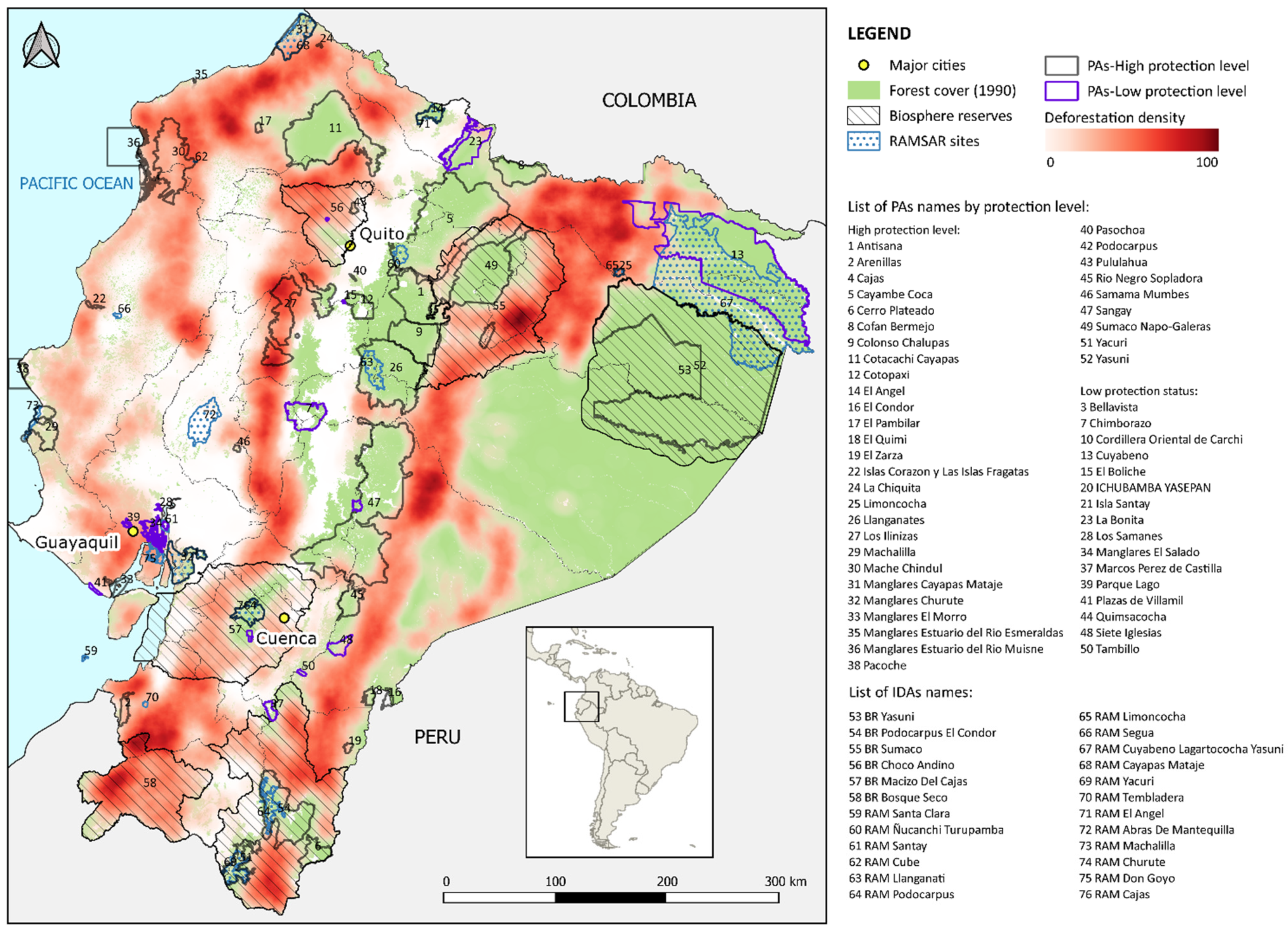
3.1. Deforestation Hotspots

Deforestation hotspots (high deforestation densities) are located along the northern coastline, along the Andes slopes throughout the country and in the northern Amazon Basin (Figure 2). In Ecuador’s PAs under SNAP, deforestation is happening mainly along the PA boundaries but also inside the PAs, as in the Mache-Chindul Ecological Reserve and Los Illinizas Ecological Reserve. In addition, protection from deforestation of Ecuador´s six mainland BRs is weak. Five BRs represent major national deforestation hotspots. Among the BRs, only Yasuni BR seems to be less affected.

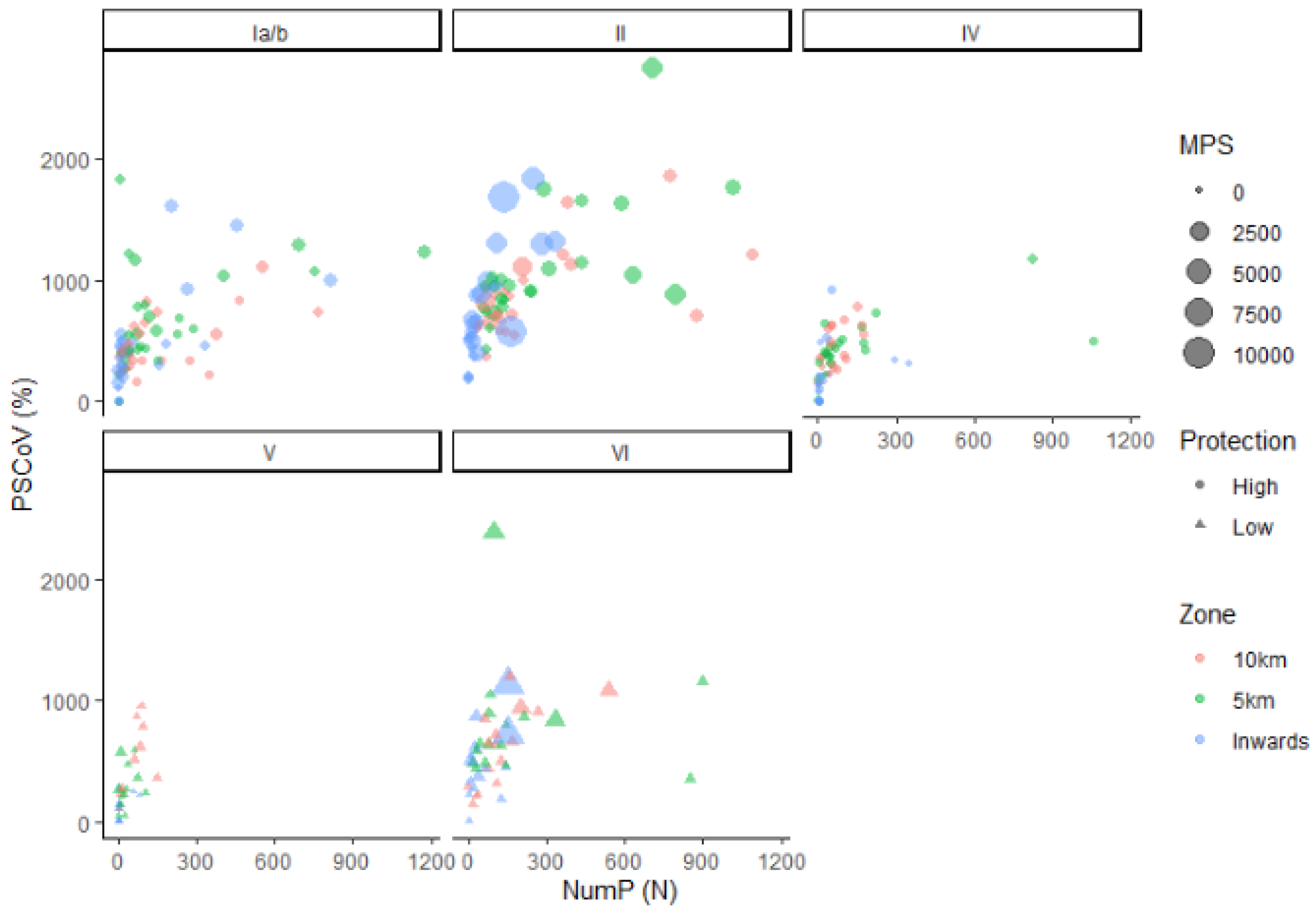
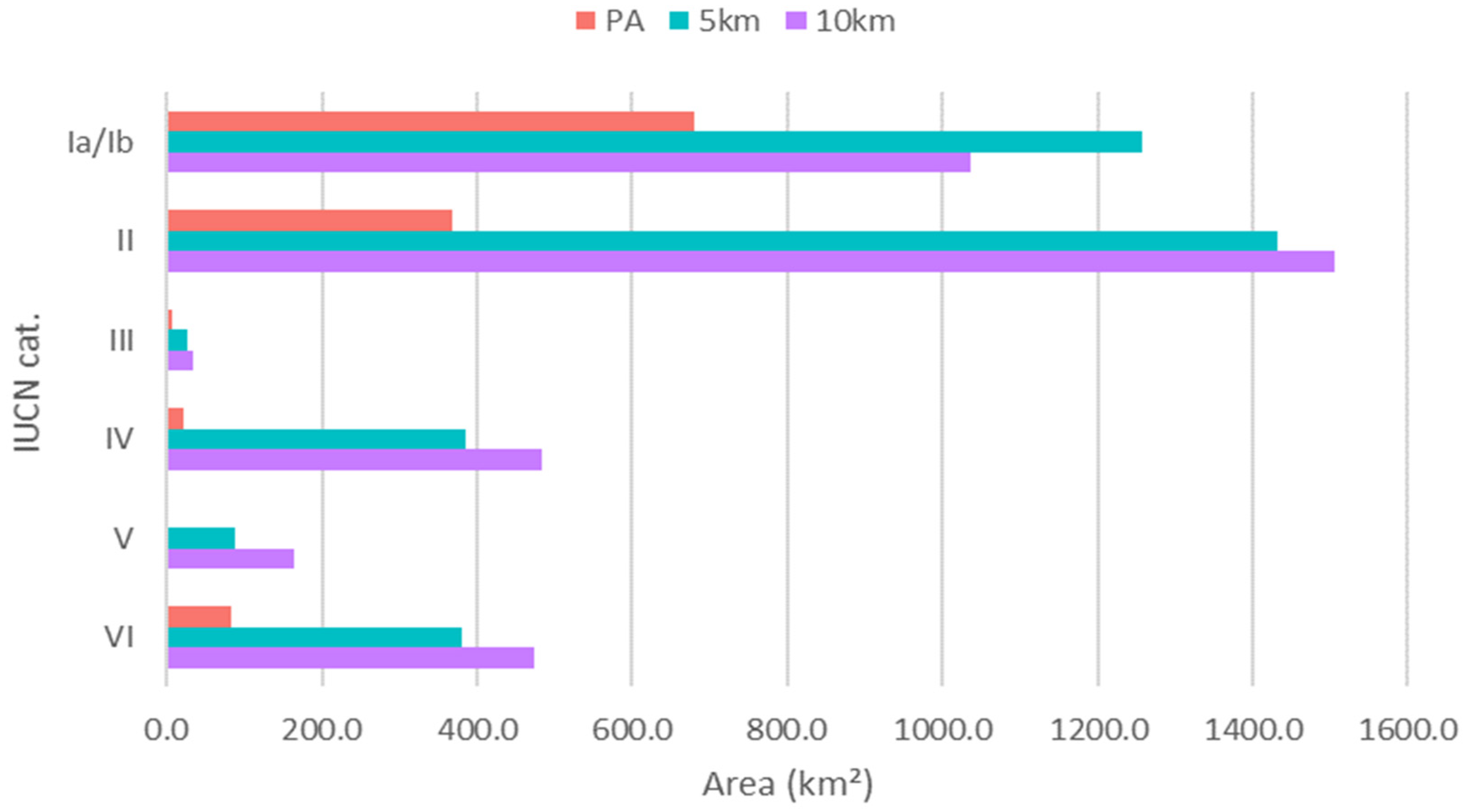
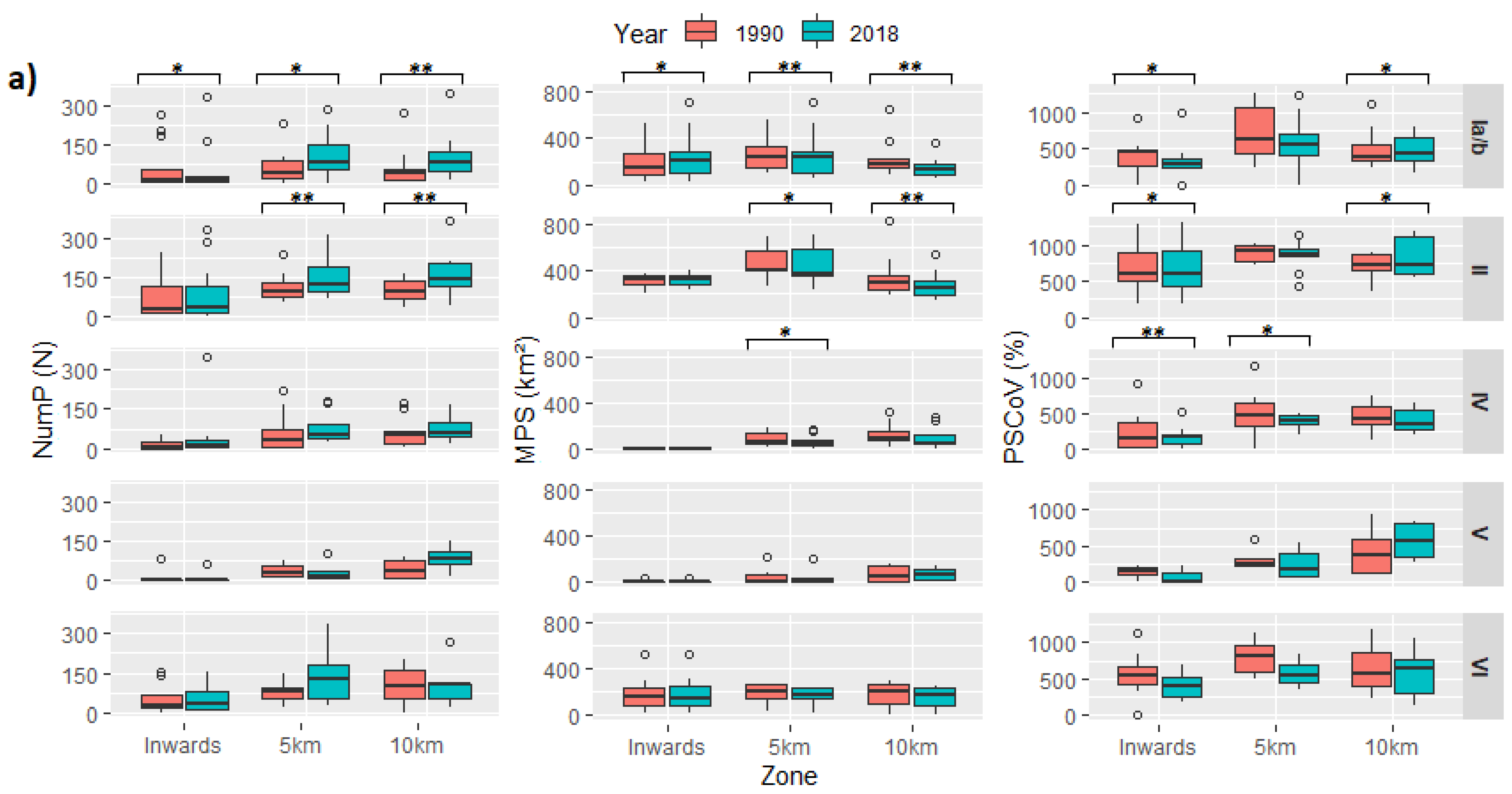
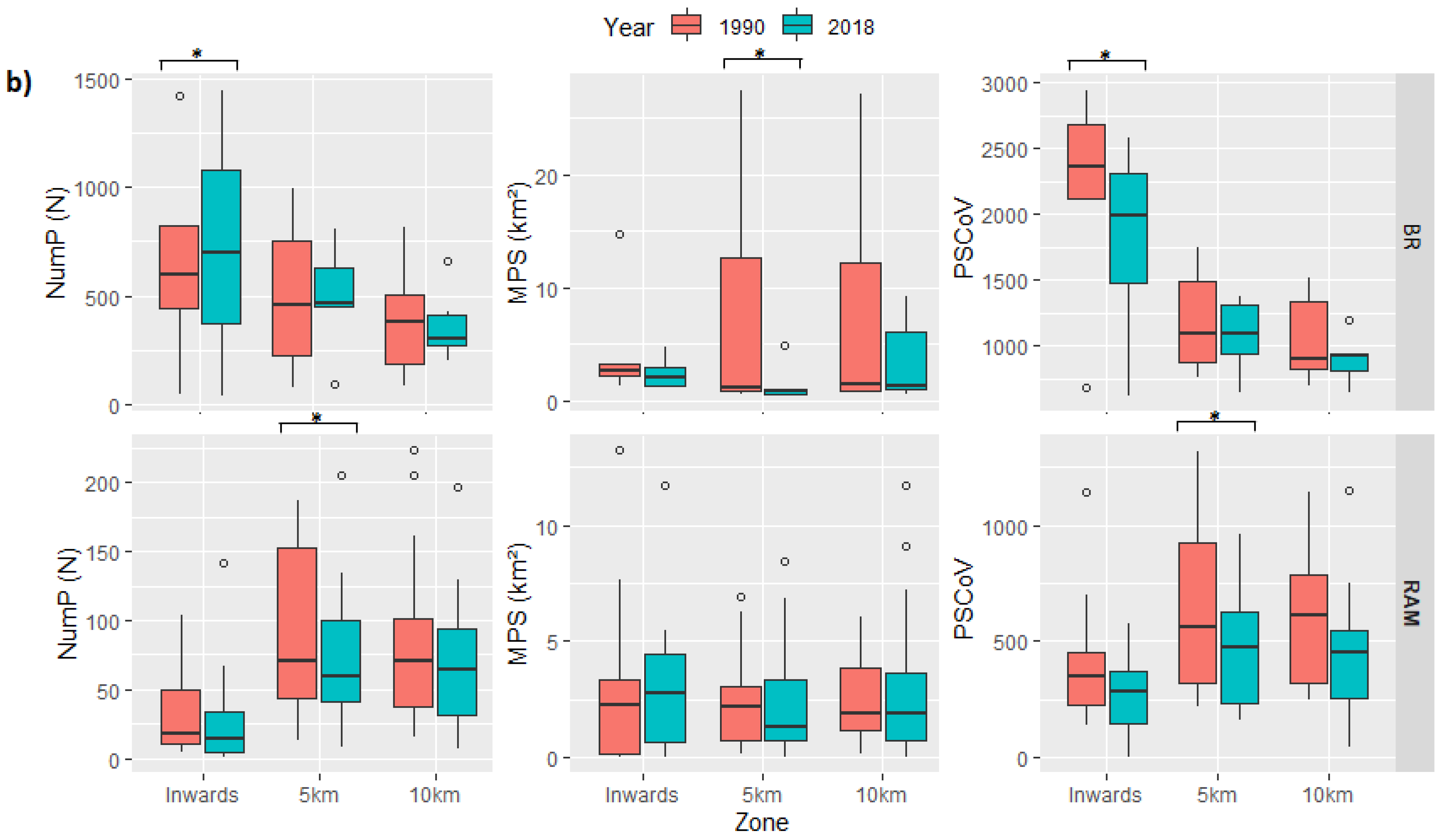
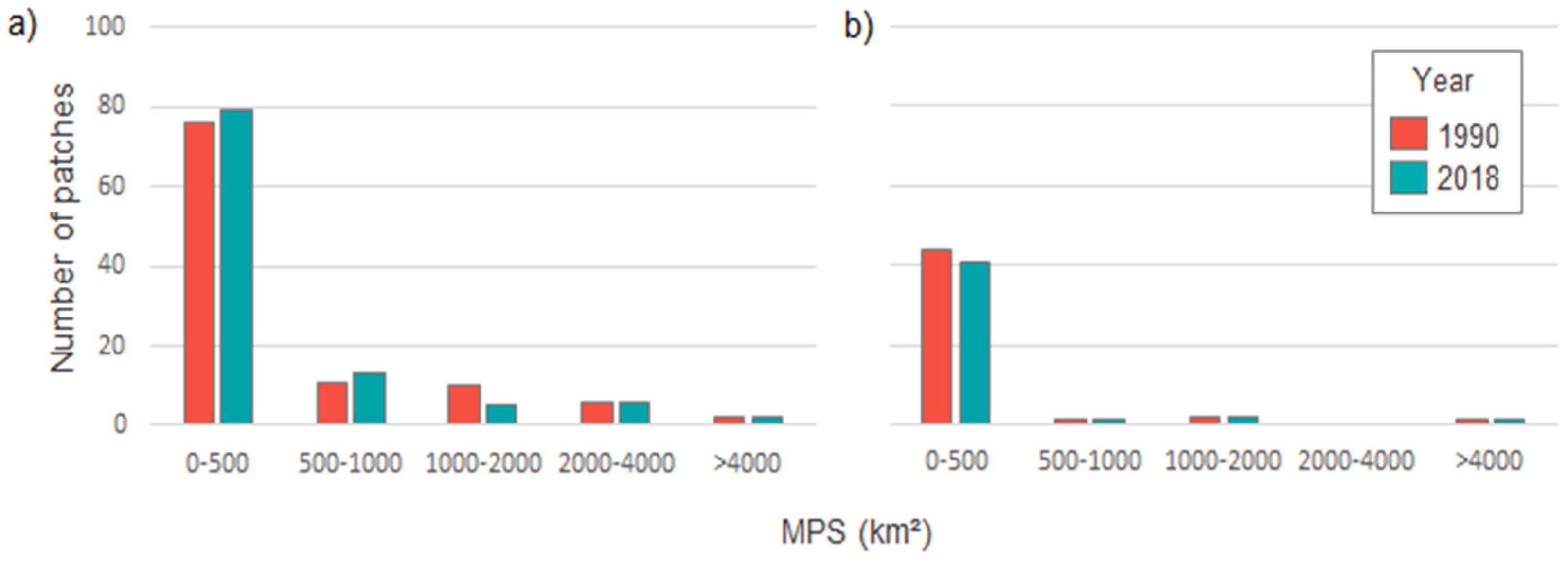
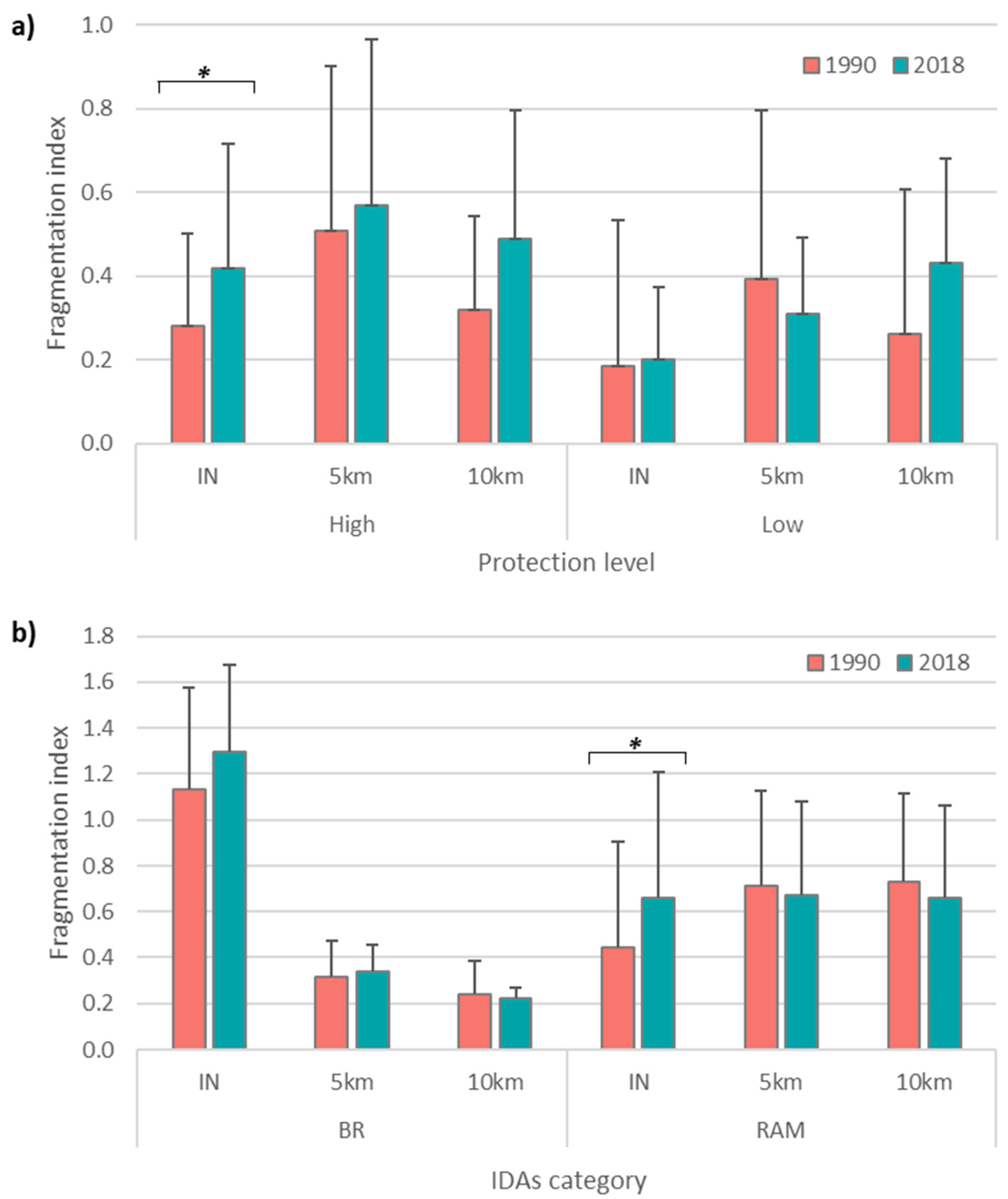
3.2. Deforestation Rates and Patterns Inside Protected Areas and Buffer Zones

Among the PAs of SNAP, those with the highest protection level (IUCN eq. cat. Ia/b and II, including buffer zones) had the highest share of national deforestation between 1990 and 2018 (see

Table 3. Proportion of deforested area to total deforestation from 1990 to 2018, in protected areas (PAs) according to IUCN equivalent categories, and international designated areas (IDAs = Biosphere reserves—BR and Ramsar sites—RAM). See Figure 3 for the total accumulated deforested area in PAs in km². SNAP= Sistema Nacional de Áreas Protegidas.

Protection Level	IUCN eq. cat.	Zone
		Within PAs, in %	5 km, in %	10 km, in %
High	Ia/Ib	2.27	4.20	3.46
	II	1.23	4.78	5.03
	III	0.03	0.09	0.11
	IV	0.07	1.29	1.61
Low	V	0.01	0.30	0.55
	VI	0.28	1.27	1.58
	TOTAL SNAP	3.89	11.93	12.34
Mixed	BR	19.37	4.69	4.51
	RAM	0.62	1.94	3.53
	TOTAL IDAs	19.99	6.63	8.04

The bold highlights the summary of SNAP and the summary of IDAs (in order to distinguish two different/independent results in one table).

; and Figure 3 for the total accumulated deforested area in PAs in km²). However, the overall highest share of national deforestation was found for BRs where almost 20% of the total deforestation of Ecuador occurred (Table 3). Approximately 4% (approx. 1163 km²) of the accumulated deforestation of PAs with IUCN eq. cat. occurred inside PAs, and up to 25.5% in their buffer zones. Including IDAs in the accumulated deforestation rate, the value increased to 24% inside PAs and 39% in their buffer zones. The three zones analyzed in this study (within PAs, 5 km and 10 km buffer) had different levels of fragmentation. In all cases, the number of deforestation patches were higher in buffer zones implying a higher prevalence of deforestation outside the boundaries of PAs (see Figure 4). The annual deforestation rates ranged from 0.30% to 0.75% during 1990 to 2018, the decreasing mean patch size and the increasing number of patch isolation of forest fragments showed that the most proximate areas to the PAs boundary (5 km buffer zone) have suffered a major amount of deforestation, especially in the year 2018. This means that next to native forest areas left for conservation, small fragments of forest have tended to disappear being replaced by other land cover types, while the large fragments have been degraded into smaller patches, drastically increasing the amount of pressure on native forests. The fragmentation index (FI) shows that the highest fragmentation took place inside BRs. The FI is also higher for PAs of IUCN eq. cat. Ia/b and II than for PAs with lower protection level (Figure 5). In addition, the FI shows that fragmentation has mainly increased in 2018 in relation to 1990, apart from RAM buffer zones and the 5 km buffer of lower PAs. Specific PAs among SNAP that experienced major deforestation inside and next to the PAs were Mache-Chindul Ecological Reserve and Los Illinizas Ecological Reserve as seen in Figure 2 and

Table A5. Fragmentation index calculated for protected areas of SNAP (the national system of protected areas) and international designated areas (IDAs) of continental Ecuador; for each zone (inside PAs, 5 km buffer, 10 km buffer). These values were averaged and classified as “Low (<1)–Medium (<2)–High (≥2)” to provide an overview of the fragmentation index among the three zones. The fragmentation index was calculated by normalizing and adding the landscape metrics NumP (Number of patches), MPS (Median Patch Size), and PSCOV (Patch Size Coefficient of Variance). The date of establishment was taken from http://ide.ambiente.gob.ec/mapainteractivo (delineation and information about protected areas in Ecuador provided by the Ministerio del Ambiente, Agua y Transición Ecológica de la República del Ecuador; accessed on 31 August 2021). IDAs = Biosphere Reserves (BRs) and Ramsar sites (RAMs). RAM Santa Clara is a marine/coastal PA and not mentioned here.

Designation	Name	Date of Establishment	Zone			Average	Fragmentation Level
			In PAs	5 km	10 km
SNAP	Antisana	1993	0.38	0.42	0.43	0.41	Low
	Arenillas	1994	0.19	0.46	0.33	0.33	Low
	Cajas	1977	0.3	0.68	0.79	0.59	Low
	Cayambe Coca	1970	1.13	0.98	0.52	0.88	Low
	Cerro Plateado	2010	0.27	0.26	0.3	0.28	Low
	Chimborazo	1987	0.27	0.42	0.47	0.39	Low
	Cofan Bermejo	2002	0.48	0.46	0.24	0.39	Low
	Colonso Chalupas	2014	0.49	0.29	0.23	0.34	Low
	Cotacachi Cayapas	1968	0.69	1.35	1.57	1.20	Medium
	Cotopaxi	1975	0.3	0.29	0.41	0.33	Low
	Cuyabeno	1979	0.7	0.67	1.03	0.80	Low
	El Angel	1992	0.22	0.54	0.54	0.43	Low
	El Boliche	1979	0	0.03	0	0.01	Low
	El Condor	1999	0.08	0.43	0.27	0.26	Low
	El Pambilar	2010	0.1	0.25	0.27	0.21	Low
	El Quimi	2006	0.3	0.28	0.36	0.31	Low
	El Zarza	2006	0.11	0.23	0.31	0.22	Low
	Isla Santay	2010	0.09	0.03	0	0.04	Low
	Islas Corazon y Las Islas Fragatas	2002	0.13	0.32	0.26	0.24	Low
	La Bonita	2017	0.36	0.32	0.16	0.28	Low
	La Chiquita	2003	0.12	0.35	0.45	0.31	Low
	Limoncocha	1985	0.18	0.29	0.24	0.24	Low
	Llanganates	1996	0.52	0.69	0.4	0.54	Low
	Los Ilinizas	1996	1.1	1.45	1.05	1.20	Medium
	Los Samanes	2010	0	0.09	0.17	0.09	Low
	Machalilla	1979	0.62	0.55	0.48	0.55	Low
	Mache Chindul	1996	1.09	1.15	0.95	1.06	Medium
	Manglares Cayapas Mataje	1995	0.4	0.45	0.3	0.38	Low
	Manglares Churute	1979	0.22	0.24	0.12	0.19	Low
	Manglares El Morro	2007	0.11	0.35	0.46	0.31	Low
	Manglares El Salado	2003	0.15	0.31	0.26	0.24	Low
	Manglares Estuario del Rio Esmeraldas	2008	0.04	0.14	0.2	0.13	Low
	Manglares Estuario del Rio Muisne	2008	0.4	0.75	0.29	0.48	Low
	Pacoche	2008	0.33	0.3	0.37	0.33	Low
	Parque Lago	2003	0.17	0.21	0.29	0.22	Low
	Pasochoa	1996	0.8	0.75	0.79	0.78	Low
	Plazas de Villamil	2011	0	0.29	0.56	0.28	Low
	Podocarpus	1982	0.64	1.25	0.93	0.94	Low
	Pululahua	1966	0.12	0.31	0.32	0.25	Low
	Quimsacocha	2012	0.11	0.38	0.57	0.35	Low
	Rio Negro Sopladora	2018	0.24	0.44	0.46	0.38	Low
	Samama Mumbes	2016	0.06	0.21	0.15	0.14	Low
	Sangay	1975	1.14	1.9	1.66	1.57	Medium
	Siete Iglesias	2012	0.2	0.67	0.81	0.56	Low
	Sumaco Napo-Galeras	1994	0.65	0.78	0.84	0.76	Low
	Tambillo	2018	0.13	0.29	0.46	0.29	Low
	Yacuri	2010	0.41	0.65	0.46	0.51	Low
	Yasuni	1979	1.35	0.71	0.83	0.96	Low
IDAs	BR Yasuni	1989	1	0.18	0.3	0.49	Low
	BR Sumaco	2000	1.48	0.43	0.21	0.71	Low
	BR Podocarpus El Condor	2007	1.79	0.47	0.25	0.84	Low
	BR Macizo Del Cajas	2013	1.59	0.22	0.22	0.68	Low
	BR Choco Andino	2018	0.66	0.44	0.23	0.44	Low
	BR Bosque Seco	2014	1.26	0.98	0.83	1.02	Medium
	RAM Yacuri	2012	0.68	0.87	0.74	0.76	Low
	RAM Tembladera	2011	0.06	0.18	0.46	0.23	Low
	RAM Segua	2000	0.13	0.16	0.19	0.16	Low
	RAM Santay	2000	0.22	0.2	0.15	0.19	Low
	RAM Podocarpus	2012	0.68	1.6	1.48	1.25	Medium
	RAM Nucanchi Turupamba	2006	1.04	0.71	0.72	0.82	Low
	RAM Machalilla	1990	0.33	0.97	0.65	0.65	Low
	RAM Llanganati	2008	0.75	0.78	0.73	0.75	Low
	RAM Limoncocha	1998	0.3	0.48	0.58	0.45	Low
	RAM El Angel	2012	0.67	0.86	0.89	0.81	Low
	RAM Don Goyo	2012	0.29	0.44	0.41	0.38	Low
	RAM Cuyabeno Lagartococha Yasuni	2017	2.33	1.3	1.17	1.60	Medium
	RAM Cube	2002	0.2	0.41	0.7	0.44	Low
	RAM Churute	1990	0.57	0.43	0.28	0.43	Low
	RAM Cayapas Mataje	2003	0.75	0.72	0.57	0.68	Low
	RAM Cajas	2002	1.19	1.12	1.46	1.26	Medium
	RAM Abras De Mantequilla	2000	0	0.14	0.05	0.06	Low

. In addition, high values of the FI were shown for the Cotacachi Cayapas National Park and Sangay National Park among SNAP. Lowest fragmentation was shown for the recreational area El Boliche.

Regarding PA effectiveness, deforested area before and after PA establishment were compared.

Table 4. Changes in deforested area before and after protected area (PA) establishment according to IUCN equivalent categories (SNAP = Sistema Nacional de Áreas Protegidas) and international designated areas (IDAs = Biosphere reserves and Ramsar sites). Changes are displayed in average deforested area in km² per year and share of deforested area (%) of total PA per year.

Protected Areas (PA) Group	Before PA Establishment: Average Deforested Area in km2 per Year (%)	After PA Establishment: Average Deforested Area in km2 per Year (%)
PA established ≤ 1989	-	15.9 (0.05)
PA established 1990–1999	-	15.3 (0.17)
PA established 2000–2007	0.3 (0.03)	0.8 (0.08)
PA established 2008–2013	0.9 (0.04)	0.6 (0.03)
PA established 2014–2017	0.3 (0.02)	-
PA established ≥ 2018	0.7 (0.11)	-
TOTAL SNAP average	0.6 (0.05)	8.2 (0.08)
IDA established ≤ 1989 *	-	0.9 (0.01)
IDA established 1990–1999	-	1.82 (0.29)
IDA established 2000–2007	132.7 (0.58)	84.2 (0.37)
IDA established 2008–2013	30.1 (0.36)	23.5 (0.22)
IDA established 2014–2017	67.2 (0.53)	-
IDA established ≥ 2018 *	17.9 (0.62)	-
TOTAL IDAs average	62.0 (0.52)	27.6 (0.22)

* only one protected area.

shows the differences per time period of PA establishment period (average deforested area in km² per year and share of deforested area of total PA area per year). Comparing the average deforested area per year for SNAP, values for PAs established ≤1989 and 1990–1999 were higher than for PAs established in other time periods. The total deforested area of PAs established ≤1989 was 446.5 km² and for PAs established 1990–1999, the deforested area was 428.3 km² after PA establishment. The total PA area that was established in these specific time periods were also larger than in other time periods but the normalized values show that still, in average, the deforestation was higher than in other PA establishment time periods. For IDAs, deforestation after PA establishment decreased but were in total much higher than for SNAP.

3.3. Analysis of the Main Drivers of Deforestation

The multiple regression analysis has shown that the distance to agricultural area has the highest correlation to deforestation on national level (correlation coefficient of 0.32) and inside PAs only (correlation coefficient of 0.45;

Table 5. Results of the multiple regression analysis at a national scale. The results of the biome levels are shown in the Table A2, Table A3 and Table A4.

Coefficients	Explanatory Share	Estimate	Std. Error	t Value	Pr (>|t|)
Roads	0.26	−5.398 × 105	3.627 × 106	−14.883	<2 × 1016 ***
Settlements	0.17	3.644 × 105	3.370 × 106	10.814	<2 × 1016 ***
Agriculture	0.32	−4.260 × 104	8.161 × 106	−52.197	<2 × 1016 ***
Plantations	0.06	7.142 × 106	3.239 × 107	22.053	<2 × 1016 ***
Rivers	0.01	5.918 × 105	7.339 × 106	8.064	7.53 × 1016 ***
Lakes	0.04	8.177 × 106	4.783 × 107	17.097	<2 × 1016 ***
Touristic infrastructure	0.18	−1.650 × 105	9.293 × 107	−17.758	<2 × 1016 ***
Mining concessions	0.20	−7.537 × 106	1.225 × 106	−6.152	7.71 × 1010 ***
Slope (topography)	0.06	−1.912 × 102	1.363 × 103	−14.023	<2 × 1016 ***

Significance levels: 0 ‘***’.

and

Table 6. Results of the multiple regression analysis in protected areas in Ecuador.

Coefficients	Explanatory Share	Estimate	Std. Error	t Value	Pr (>|t|)
Roads	0.34	−6.387 × 105	3.251 × 106	−19.644	<2 × 1016 ***
Settlements	0.28	−2.548 × 105	2.506 × 106	−10.170	<2 × 1016 ***
Agriculture	0.45	−3.826 × 104	5.432 × 106	−70.441	<2 × 1016 ***
Plantations	0.27	−9.805 × 106	3.802 × 107	−25.787	<2 × 1016 ***
Rivers	0.13	−2.920 × 105	1.092 × 105	−2.675	0.00748 **
Lakes	0.08	6.753 × 106	5.978 × 107	11.296	<2 × 1016 ***
Touristic infrastructure	0.27	1.630 × 105	1.118 × 106	14.587	<2 × 1016 ***
Mining concessions	0.19	3.641 × 105	1.535 × 106	23.713	<2 × 1016 ***
Slope (topography)	0.01	−1.689 × 102	1.207 × 103	−13.999	<2 × 1016 ***

Significance levels: 0 ‘***’ 0.001 ‘**’.

). On the national level, deforestation is also more prevalent in the proximity of roads (0.26) and mining concessions (0.20). Each independent variable presents a high level of significance for the model and an adjusted R-squared of 0.1306. In PAs, besides agricultural areas, deforestation occurs more often next to roads (0.34), settlements (0.28), plantations (0.27) and tourist infrastructure (0.27). The adjusted R-squared is 0.2308.

Agriculture is also the main driver of deforestation on biome level (

Table A2. Results of the Multiple Regression Analysis of the coastal biome.

Coefficients	Explanatory Share	Estimate	Std. Error	t Value	Pr (>|t|)
Roads	0.11	−7.404 × 105	1.111 × 105	−6.665	2.67 × 1011 ***
Settlements	0.05	4.807 × 105	3.901 × 106	12.323	<2 × 1016 ***
Agriculture	0.20	−5.359 × 104	1.665 × 105	−32.190	<2 × 1016 ***
Plantations	0.07	−1.742 × 105	1.755 × 106	−9.926	<2 × 1016 ***
Rivers	0.01	5.727 × 105	5.248 × 106	10.913	<2 × 1016 ***
Lakes	0.15	1.200 × 105	5.152 × 107	23.303	<2 × 1016 ***
Touristic infrastructure	0.06	2.140 × 105	1.566 × 106	13.666	<2 × 1016 ***
Mining concessions	0.06	−2.318 × 105	1.449 × 106	−15.991	<2 × 1016 ***
Slope (topography)	0.06	1.867 × 102	1.583 × 103	11.791	<2 × 1016 ***

Significance codes: 0 ‘***’.

,

Table A3. Results of the Multiple Regression Analysis of the Andes biome.

Coefficients	Explanatory Share	Estimate	Std. Error	t Value	Pr (>|t|)
Roads	0.01	−7.026 × 105	8.850 × 106	−7.939	2.07 × 1015 ***
Settlements	0.07	9.506 × 105	3.458 × 106	27.491	<2 × 1016 ***
Agriculture	0.31	−1.315 × 103	2.053 × 105	−64.056	<2 × 1016 ***
Plantations	0.13	6.764 × 105	1.850 × 106	36.567	<2 × 1016 ***
Rivers	0.09	−4.125 × 104	1.926 × 105	−21.416	<2 × 1016 ***
Lakes	0.13	6.943 × 106	6.488 × 107	10.701	<2 × 1016 ***
Touristic infrastructure	0.04	−3.166 × 105	1.837 × 106	−17.236	<2 × 1016 ***
Mining concessions	0.13	−8.439 × 105	3.581 × 106	−23.565	<2 × 1016 ***
Slope (topography)	0.06	−5.248 × 103	1.251 × 103	−4.195	2.74 × 105 ***

Significance codes: 0 ‘***’.

and

Table A4. Results of the Multiple Regression Analysis of the Amazon biome.

Coefficients	Explanatory Share	Estimate	Std. Error	t Value	Pr (>|t|)
Roads	0.36	−7.404 × 105	1.111 × 105	−6.665	2.67 × 1011 ***
Settlements	0.33	4.807 × 105	3.901 × 106	12.323	<2 × 1016 ***
Agriculture	0.41	−5.359 × 104	1.665 × 105	−32.190	<2 × 1016 ***
Plantations	0.06	−1.742 × 105	1.755 × 106	−9.926	<2 × 1016 ***
Rivers	0.02	5.727 × 105	5.248 × 106	10.913	<2 × 1016 ***
Lakes	0.06	1.200 × 105	5.152 × 107	23.303	<2 × 1016 ***
Touristic infrastructure	0.32	2.140 × 105	1.566 × 106	13.666	<2 × 1016 ***
Mining concessions	0.30	−2.318 × 105	1.449 × 106	−15.991	<2 × 1016 ***
Slope (topography)	0.08	1.867 × 102	1.583 × 103	11.791	<2 × 1016 ***

Significance codes: 0 ‘***’.

). For the coastal biome, agriculture shows a correlation coefficient of 0.20, followed by lakes and roads with coefficient values of 0.15 and 0.11, respectively (Table A2). For the Andes biome, agriculture has a correlation coefficient of 0.31, followed by forest plantations, lakes, and mining concessions with a coefficient value of 0.13 (Table A3). For the Amazon biome, agriculture has a correlation coefficient of 0.41, followed by roads, settlements, tourist places, and mining concessions with coefficient values of 0.36, 0.33, 0.32, and 0.30 respectively (Table A4).

4. Discussion

4.1. Deforestation and Protected Areas in Ecuador

The analysis of PA effectiveness has shown that deforested area marginally increased for SNAP and decreased for IDAs after PA establishment. The deforested area was in general higher for IDAs than for SNAP. Therefore, the results suggest that PAs of SNAP are generally effective at preventing deforestation within their boundaries. However, forest fragmentation is higher inside PAs with higher protection status than areas of lower protection status. This finding is in contrast to van der Hoek [40] where no effects were found between the age, size, and level of protection but he considered only the time frame between 2000 and 2008 and 19 national PAs.

Especially the Ecological Reserves Mache-Chindul and Los llinizas (IUCN cat. equiv. Ia/b) have high deforestation rates. Mache-Chindul is confronted with high population densities and human activities inside and next to the PA [78]. In addition, the National Parks Sangay and Cotacachi Cayapas (IUCN cat. equiv. II) have high protection status but receive major forest fragmentation. This development could be related to better accessibility due to roads as it is the case in the Amazon biome [79]. A fragmentation analysis by the Ministry of Environment has revealed that fragmentation in the Amazon is mainly along the rivers that are used as main transportation routes and accessibility in dense forest [69]. In addition, landowners retain their ownership of areas within PAs where nature conservation might not be the primary aim [80]. A lack of protection and control might be also explained historically, where the national government was lacking funding to regulate human activities within PAs as a consequence of a crisis in 2000 ([80]; citing [81]). Other national parks in Ecuador seem to have a relatively good protection status. Negru et al. [82] analyzed the management effectiveness of Ecuador’s national parks where Galapagos National Park had the highest management effectiveness and Río Negro Sopladora National Park had the lowest because of a lack of management plans, among others. However, the findings might be related to the fact that the National Park Río Negro Sopladora has been just established in 2018 [83]. The reason for its newly established protection was also the high threat of human activities, especially by cattle farming [84]. Galapagos National Park had the highest resources available. In contrast, Sangay National Park had the second lowest values of all management effectiveness indicators (context, planning, inputs, process, outputs and outcomes; for more details, see Leverington et al. [85]) which also reflects our findings that deforestation is entering the PA zone in this case. In addition, BRs belong to the deforestation hotspots in Ecuador. BRs are areas with lower protection status where a balanced human land use besides ecosystem protection is allowed. However, it has to be considered that conservation was not in place for a long time because most of the BRs of continental Ecuador were established just after the year 2000, except for Yasuni BR (established in 1989 [86]) and Sumaco BR (established in 2000 [87]). Furthermore, some IDAs and SNAP are overlapping in their conservation status that may result in a decreased effectiveness of conservation measures and a lack of clarity around the governance and enforcement of management actions, hindering their purpose for conserving biodiversity [88]. Despite the fact that SNAP covers a considerable area of Ecuador’s natural forest, still large gaps remain in their coverage of global biodiversity hotspots (i.e., Tumbes-Chocó-Magdalena [89]), either with no or only a few PAs and BRs with low protection status [90].

We identified agriculture as the main driver of deforestation on national level, biome level and in PAs. This variable has the highest correlation coefficient in all the models with 0.32 at national scale, 0.31 for the Andes, 0.20 for the Coast, and 0.41 for the Amazon. Agriculture is a prominent driver of deforestation in South America. For example, in Brazil, especially soy production is causing deforestation today [91]. The global map of forest loss by Curtis et al. [92] shows in Ecuador, Peru, Bolivia, Colombia, Venezuela, and northern Brazil a forest loss due to shifting cultivation and commodity production. Agriculture is also the main driver of deforestation in PAs, confirmed by Jayathilake et al. [93] who analyzed 28 tropical conservation landscapes. Agricultural activities within the Ecuadorian Amazon make up almost 60% of income ([94] citing [95]). The main uses of agricultural areas in this biome are pastures cultivated for livestock and permanent and transitory crops. For instance, permanent crops as main drivers of deforestation are the African palm, cocoa, and palm heart, while transitory crops are the corn and cassava in the Amazon [48]. According to the United States Department of Agriculture, Ecuador is the eleventh-largest palm oil producer worldwide. In South America, Ecuador is the second largest, after Colombia [96]. Most of the palm oil from Ecuador comes from the Coast/Choco region [94]. Agricultural activities in the coastal biome are especially concentrated in Esmeraldas Province [36,97] and mainly related to pastures for livestock and permanent crops/plantations of African palm, cocoa, and banana for international trade [48]. In the case of the Andes, deforestation is mainly caused by agriculture such as pastures cultivated for livestock but on a smaller scale than in the Amazon and the Coast, followed by transitory crops, fallow lands, and permanent crops [36,48]. For instance, transitory crops such as corn, potatoes, and barley, and permanent crops such as sugar cane, cocoa, tree tomato, and piedmont heart palm are characteristic in this biome.

The other drivers of deforestation identified in the multiple regression analysis were distances to mining concessions, settlements, touristic infrastructure, plantations, and roads. For example, for mining concessions, in 2016, the national government allowed mining exploration of about 13% of continental Ecuador resulting in more deforestation [44]. However, already before 2016, there was in the Amazon a major forest loss between 2000 and 2015, especially in indigenous lands, due to the legal and illegal mining [98]. The largest number of mines are situated in the south of the country, both in the provinces of Morona Santiago and Zamora Chinchipe in the Amazon, and in the province of Loja in the Andes [23,54]. This corroborates the results obtained in the model, where the Amazon and the Andes are the biomes with high impact of deforestation by mining. In addition, urban expansion and demographic development play an important role in deforestation. Forests are directly affected by the high demand for land and resources for the development of settlements and infrastructure [99,100,101]. Roads also play a role in improved accessibility to forests for logging. The multiple regression analysis indicated that forests are affected by these driving forces at national scale, especially on the Coast and in the Amazon [79]. Plantations and touristic infrastructure were additional drivers especially in PAs. The development of tourism is often an issue where mass tourism and tourism without ecological considerations can potentially occur. The construction of tourist infrastructure and facilities such as lodging is the main cause of deforestation, especially in the vicinity of protected areas [102]. For example, the Guayacanes forest and the forest of Puyango in the south of the country are negatively affected by tourism [103,104]. Regarding forest plantations, in almost thirty years, teak, melina, balsa, eucalyptus, and pine have tripled and have affected the native forest. Approximately, 180,000 hectares of commercial forest plantations have been registered in 2019, especially on the Coast and the Andes of the country [50,105]. Another pressure in PAs that may not cause deforestation but a loss of biodiversity is hunting. Naughton-Treves et al. [22] detected hunting as the most widespread human forest use besides logging, livestock and mining in 15 forest parks in Ecuador and Peru even though PAs were partially assigned with strict protection status.

Our findings can serve as input for a National Ecosystem Assessment in Ecuador and ecosystem protection programs, e.g., the development of National Biodiversity Strategies and Action Plans of the Convention on Biological Diversity (CBD [106]), the United Nations Framework Convention on Climate Change (UNFCCC; in the frame of REDD+ [107]), as national input for the Intergovernmental Platform on Biodiversity and Ecosystem Services (IPBES [108]) and to reach the Sustainable Development Goals (SDGs), specifically Goal 15.2 by “2020, promote the implementation of sustainable management of all types of forests, halt deforestation, restore degraded forests and substantially increase afforestation and reforestation globally” [109]. The findings could also support assessments regarding the effectiveness of PAs of different protection status. Forest loss, fragmentation, and degradation are still continuing. More political commitment is needed to reverse the negative trend of forest loss. More substantive protection of ecosystems in general but specifically for forest ecosystems is needed [34,110]. Even though conservation control might be improved, it could shift deforestation to other places that are not or less protected. These leakage patterns on areas surrounding PAs can undermine conservation strategies to sustain biodiversity [111]. The Socio Bosque Program (SBP) is one of the national financial incentives to protect biodiversity but also to improve people’s living conditions. Owners of private and communal lands are paid for the conservation and management of protected areas [112]. Cuenca et al. [40] assessed the SBP on the national level and they could detect that this program avoided about 1.5% deforestation in areas of direct payments. Furthermore, Cuenca et al. [40] reported that individual SBP beneficiaries had a more significant impact on avoiding deforestation than community PSB beneficiaries. This was due to the fact that individual beneficiaries were located closer to the hotspots of deforestation.

4.2. Methodological Discussion

The methodological approach of this study could support, for example, the measurement of the progress of the SDGs. The “forest area annual net change rate” and the “proportion of forest area within legally established protected areas” belong to the SDG Global Monitoring Indicators [113]. National forest monitoring systems can complement international efforts [114]. However, the spatially explicit approach is highly dependent on data availability, access and accuracy [115,116]. Data gaps occurred for drivers of forest loss that are not easily identified by remote sensing or where data was not available, e.g., climate change, hunting and soil pollution. However, regarding climate change, Manchego et al. [117] identified that annual forest loss rate due to human land conversion was significantly higher than the losses in an extreme climate change scenario in the Tumbes-Piura dry forests. Furthermore, indirect drivers could play a role but they are difficult to be identified by remote sensing and GIS. Indirect drivers of change are complex interactions of social, economic, political, cultural, and technological processes that might be related to international, national, or local levels, e.g., political incentives and economic interest [118,119].

Additional data uncertainties might have been occurred in the assessment of deforestation before and after PA establishment (Table 4) because of missing information about deforestation before 1990 and after 2018. And for IDAs established ≤1989 and ≥2018, there was only one IDA considered respectively. Uncertainties also exist in the data of the multiple regression analysis where only one-time step and potentially outdated data was used due to missing spatial information about the current status, e.g., for touristic infrastructure generated in 2002 or rivers and lakes updated in 2013. On the other hand, most of the spatial information obtained is referenced to 2018 or the current year, e.g., LULC data from 2018, deforestation rate between 1990 and 2018 and updated roads in 2020. Nevertheless, these temporal differences in datasets could lead to uncertainty in the results.

Spatial analyses could be combined with field data and stakeholder interviews in order to identify in more detail the complex interactions between the location and level of deforestation, drivers and consequences [120,121]. The spatial assessment of the effectiveness of PAs could be expanded to other indicators such as human population density and the percentage of agricultural area inside PAs [122]. The assessment of PA effectiveness could be further combined with surveys, e.g., evaluation criteria for BRs [123].

For the classification of PAs according to the IUCN categories, we followed the suggestions by Boitani et al., Dudley, and Leroux et al. [59,60,61]. However, classification is not standardized. For example, Naughton-Treves et al. [22] assigned the IUCN-VI category differently but the paper was published before the suggestion provided by MAATE [58]. The publication of MAATE [58] is to our knowledge the last updated version about Ecuador´s PA assignment according to the IUCN classification. Furthermore, national and international protection status of some PAs are overlapping. For example, Yasuni was a national park but at the same time part of a BR. The same for the RAMs Cayapas Mataje and El Angel that have also a high protection status in SNAP.

5. Conclusions

The spatial analysis of deforestation (Section 3.1) and fragmentation analyses (Section 3.2) have shown that highest levels of deforestation between 1990 and 2018 was taking place inside BRs but findings might be biased because most of the areas that are BRs today were not PAs in 1990. However, PAs that are part of BRs today were already PAs of higher protection levels in 1990. Therefore, even though PAs were in place in 1990, deforestation was higher than expected in our analysis between 1990 and 2018. Considering SNAP, the prevention from deforestation of most of the PAs is effective when comparing deforestation rates inside PAs and their buffer zones. Interestingly, those areas of SNAP with higher protection levels received more deforestation than those areas with lower protection that contradicts the protection efficiency. Agriculture was identified as the main driver of deforestation on national and biome level as well as in PAs (Section 3.3). Other drivers of deforestation were mining concessions, settlements, touristic infrastructure, plantations, roads and slope. This signifies that more political commitment is needed to reverse the negative trend of forest loss. There should be further consideration on how to address uncertainties of our analysis, for example, due to the classification of SNAP into IUCN equivalent categories.

References

1. Daily, G.C. (Ed.) Nature’s Services: Societal Dependence On Natural Ecosystems; Island Press: Washington, DC, USA; Covelo, CA, USA, 1997. [Google Scholar]
2. Galicia, L.; Zarco-Arista, A.E. Multiple ecosystem services, possible trade-offs and synergies in a temperate forest ecosystem in Mexico: A review. Int. J. Biodivers. Sci. Ecosyst. Serv. Manag. 2014, 10, 275–288. [Google Scholar] [CrossRef]
3. García-Nieto, A.P.; García-Llorente, M.; Iniesta-Arandia, I.; Martín-López, B. Mapping forest ecosystem services: From providing units to beneficiaries. Ecosyst. Serv. 2013, 4, 126–138. [Google Scholar] [CrossRef]
4. Myers, N. The world’s forests and their ecosystem services. In Nature’s Services: Societal Dependence on Natural Ecosystems; Daily, G.C., Ed.; Island Press: Washington, DC, USA; Covelo, CA, USA, 1997. [Google Scholar]
5. UN Environment Programme (UNEP); Food and Agriculture Organization of the United Nations (FAO). The State of the World’s Forests: Forests, Biodiversity and People; UNEP: Rome, Italy, 2020. [Google Scholar]
6. Jencso, K.G.; McGlynn, B.L.; Gooseff, M.N.; Wondzell, S.M.; Bencala, K.E.; Marshall, L.A. Hydrologic connectivity between landscapes and streams: Transferring reach- and plot-scale understanding to the catchment scale. Water Resour. Res. 2009, 45, W04428. [Google Scholar] [CrossRef] [Green Version]
7. Vié, J.-C.; Hilton-Taylor, C.; Stuart, S.N. Wildlife in a Changing World—An Analysis of the 2008 IUCN Red List of Threatened Species; IUCN: Gland, Switzerland, 2009; 157p. [Google Scholar]
8. Brook, B.W.; Sodhi, N.S.; Ng, P.K.L. Catastrophic extinctions follow deforestation in Singapore. Nature 2003, 424, 420–426. [Google Scholar] [CrossRef]
9. Giam, X. Global biodiversity loss from tropical deforestation. Proc. Natl. Acad. Sci. USA 2017, 114, 5775–5777. [Google Scholar] [CrossRef] [PubMed] [Green Version]
10. Eva, H.D.; Achard, F.; Beuchle, R.; de Miranda, E.; Carboni, S.; Seliger, R.; Vollmar, M.; Holler, W.A.; Oshiro, O.T.; Barrena Arroyo, V.; et al. Forest Cover Changes in Tropical South and Central America from 1990 to 2005 and Related Carbon Emissions and Removals. Remote Sens. 2012, 4, 1369–1391. [Google Scholar] [CrossRef] [Green Version]
11. Ochoa-Cueva, P.; Fries, A.; Montesinos, P.; Rodríguez-Díaz, J.A.; Boll, J. Spatial Estimation of Soil Erosion Risk by Land-cover Change in the Andes OF Southern Ecuador. Land Degrad. Develop. 2015, 26, 565–573. [Google Scholar] [CrossRef]
12. Anderegg, W.R.L.; Berry, J.A.; Smith, D.D.; Sperry, J.S.; Anderegg, L.D.L.; Field, C.B. The roles of hydraulic and carbon stress in a widespread climate-induced forest die-off. Proc. Natl. Acad. Sci. USA 2012, 109, 233–237. [Google Scholar] [CrossRef] [Green Version]
13. Creeden, E.P.; Hicke, J.A.; Buotte, P.C. Climate, weather, and recent mountain pine beetle outbreaks in the western United States. For. Ecol. Manag. 2014, 312, 239–251. [Google Scholar] [CrossRef]
14. Cochrane, M.A.; Barber, C.P. Climate change, human land use and future fires in the Amazon. Glob. Chang. Biol. 2009, 15, 601–612. [Google Scholar] [CrossRef]
15. Scholze, M.; Knorr, W.; Arnell, N.W.; Prentice, I.C. A climate-change risk analysis for world ecosystems. Proc. Natl. Acad. Sci. USA 2006, 103, 13116–13120. [Google Scholar] [CrossRef] [PubMed] [Green Version]
16. IUCN. The IUCN Red List of Threatened Species, Version 2021-1; Available online: https://www.iucnredlist.org/statistics (accessed on 15 November 2021).
17. Balthazar, V.; Vanacker, V.; Molina, A.; Lambin, E.F. Impacts of forest cover change on ecosystem services in high Andean mountains. Ecol. Indic. 2015, 48, 63–75. [Google Scholar] [CrossRef]
18. Cardille, J. Agricultural land-use change in Brazilian Amazônia between 1980 and 1995: Evidence from integrated satellite and census data. Remote Sens. Environ. 2003, 87, 551–562. [Google Scholar] [CrossRef]
19. Grau, H.R.; Aide, M. Globalization and land-use transitions in Latin America. Ecol. Soc. 2008, 13, 16. [Google Scholar] [CrossRef] [Green Version]
20. Walker, W.S.; Gorelik, S.R.; Baccini, A.; Aragon-Osejo, J.L.; Josse, C.; Meyer, C.; Macedo, M.N.; Augusto, C.; Rios, S.; Katan, T.; et al. The role of forest conversion, degradation, and disturbance in the carbon dynamics of Amazon indigenous territories and protected areas. Proc. Natl. Acad. Sci. USA 2020, 117, 3015–3025. [Google Scholar] [CrossRef] [Green Version]
21. Mainville, N.; Webb, J.; Lucotte, M.; Davidson, R.; Betancourt, O.; Cueva, E.; Mergler, D. Decrease of soil fertility and release of mercury following deforestation in the Andean Amazon, Napo River Valley, Ecuador. Sci. Total Environ. 2006, 368, 88–98. [Google Scholar] [CrossRef]
22. Naughton-Treves, L.; Alvarez-Berríos, N.; Brandon, K.; Bruner, A.; Holland, M.B.; Ponce, C.; Saenz, M.; Suarez, L.; Treves, A. Expanding protected areas and incorporating human resource use: A study of 15 forest parks in Ecuador and Peru. Sustain. Sci. Pract. Policy 2006, 2, 32–44. [Google Scholar] [CrossRef] [Green Version]
23. Amazon Geo-Referenced Socio-Environmental Information Network (RAISG). Pressures on and Threats to Protected Areas and Indigenous Territories in Amazonia (RAISG, São Paulo, Brasil, 2018). 2018. Available online: https://www.amazoniasocioambiental.org/en (accessed on 31 August 2021).
24. Lovejoy, T.E. Biodiversity Conservation Targets: How to Allocate Resources. One Earth 2020, 2, 415–416. [Google Scholar] [CrossRef]
25. Qin, Y.; Xiao, X.; Dong, J.; Zhang, Y.; Wu, X.; Shimabukuro, Y.; Arai, E.; Biradar, C.; Wang, J.; Zou, Z.; et al. Improved estimates of forest cover and loss in the Brazilian Amazon in 2000–2017. Nat. Sustain. 2019, 2, 764–772. [Google Scholar] [CrossRef] [Green Version]
26. Pfaff, A.; Robalino, J.; Lima, E.; Sandoval, C.; Herrera, L.D. Governance, Location and Avoided Deforestation from Protected Areas: Greater Restrictions Can Have Lower Impact, Due to Differences in Location. World Dev. 2014, 55, 7–20. [Google Scholar] [CrossRef]
27. Schleicher, J.; Peres, C.A.; Amano, T.; Llactayo, W.; Leader-Williams, N. Conservation performance of different conservation governance regimes in the Peruvian Amazon. Sci. Rep. 2017, 7, 11318. [Google Scholar] [CrossRef] [PubMed] [Green Version]
28. Lessmann, J.; Fajardo, J.; Muñoz, J.; Bonaccorso, E. Large expansion of oil industry in the Ecuadorian Amazon: Biodiversity vulnerability and conservation alternatives. Ecol. Evol. 2016, 6, 4997–5012. [Google Scholar] [CrossRef] [PubMed] [Green Version]
29. Beech, E.; Rivers, M.; Oldfield, S.; Smith, P.P. GlobalTreeSearch: The first complete global database of tree species and country distributions. J. Sustain. For. 2017, 36, 454–489. [Google Scholar] [CrossRef]
30. Calderón, M.G.S.; Reyes, C.G.P. Ecuador: Revisión a las Principales Características del Recurso Forestal y de la Deforestación; Revista Científica y Tecnológica UPSE, 2015; Available online: https://incyt.upse.edu.ec/ciencia/revistas/index.php/rctu/article/view/70/pdf_1 (accessed on 15 November 2021).
31. Curatola Fernández, G.; Obermeier, W.; Gerique, A.; López Sandoval, M.; Lehnert, L.; Thies, B.; Bendix, J. Land Cover Change in the Andes of Southern Ecuador—Patterns and Drivers. Remote Sens. 2015, 7, 2509–2542. [Google Scholar] [CrossRef] [Green Version]
32. Ministerio del Ambiente del Ecuador (MAE). Estadísticas forestales 2011–2014 Subsecretaría de Patrimonio Natural. Dirección Nacional Forestal del Ministerio del Ambiente; MAE: Quito, Ecuador, 2015.
33. Andrade-Núñez, M.J.; Aide, T.M. Using nighttime lights to assess infrastructure expansion within and around protected areas in South America. Environ. Res. Commun. 2020, 2, 21002. [Google Scholar] [CrossRef]
34. Noh, J.K.; Echeverria, C.; Kleemann, J.; Koo, H.; Fürst, C.; Cuenca, P. Warning about conservation status of forest ecosystems in tropical Andes: National assessment based on IUCN criteria. PLoS ONE 2020, 15, e0237877. [Google Scholar] [CrossRef]
35. Sierra, R.; Campos, F.; Chamberlin, J. Assessing biodiversity conservation priorities: Ecosystem risk and representativeness in continental Ecuador. Landsc. Urban Plan. 2002, 59, 95–110. [Google Scholar] [CrossRef]
36. Sierra, R.; Calva, O.; Guevara, A. La Deforestación en el Ecuador, 1990–2018: Factores Promotores y Tendencias Recientes: En el Marco de la Implementación del Programa Integral Amazónico de Conservación de Bosques y Producción Sostenible; Programa Integral Amazónico de Conservación de Bosques, Producción Sostenible PROAmazonía, Iniciativa Liderada por el Ministerio del Ambiente y Agua (MAAE): Quito, Ecuador; Ministerio de Agricultura y Ganadería (MAG): Quito, Ecuador; con apoyo del Programa de las Naciones Unidas para el Desarrollo (PNUD): Quito, Ecuador; Ministerio de Ambiente y Agua del Ecuador: Quito, Ecuador, 2021.
37. González-Jaramillo, V.; Fries, A.; Rollenbeck, R.; Paladines, J.; Oñate-Valdivieso, F.; Bendix, J. Assessment of deforestation during the last decades in Ecuador using NOAA-AVHRR satellite data. Erdkunde 2016, 70, 217–235. [Google Scholar] [CrossRef]
38. Rivas, C.A.; Guerrero-Casado, J.; Navarro-Cerillo, R.M. Deforestation and fragmentation trends of seasonal dry tropical forest in Ecuador: Impact on conservation. For. Ecosyst. 2021, 8, 46. [Google Scholar] [CrossRef]
39. Tapia-Armijos, M.F.; Homeier, J.; Espinosa, C.I.; Leuschner, C.; de La Cruz, M. Deforestation and Forest Fragmentation in South Ecuador since the 1970s—Losing a Hotspot of Biodiversity. PLoS ONE 2015, 10, e0133701. [Google Scholar] [CrossRef] [Green Version]
40. Van der Hoek, Y. The potential of protected areas to halt deforestation in Ecuador. Environ. Conserv. 2017, 44, 124–130. [Google Scholar] [CrossRef]
41. Cuenca, P.; Echeverria, C. How do protected landscapes associated with high biodiversity and population levels change? PLoS ONE 2017, 12, e0180537. [Google Scholar] [CrossRef] [PubMed] [Green Version]
42. Ministerio del Ambiente del Ecuador (MAE); Food and Agriculture Organization of the United Nations (FAO). Resultados de la Evaluación Nacional Forestal—Ecuador; MAE: Quito, Ecuador, 2014.
43. López-Sandoval, M.; Maldonado, P. Change, Collective Action, and Cultural Resilience in Páramo Management in Ecuador. Mt. Res. Dev. 2019, 39, R1. [Google Scholar] [CrossRef]
44. Encyclopædia Britannica Inc. Ecuador. Available online: https://www.britannica.com/place/Ecuador#ref25836 (accessed on 24 November 2021).
45. Roy, B.A.; Zorrilla, M.; Endara, L.; Thomas, D.C.; Vandegrift, R.; Rubenstein, J.M.; Policha, T.; Ríos-Touma, B.; Read, M. New Mining Concessions Could Severely Decrease Biodiversity and Ecosystem Services in Ecuador. Trop. Conserv. Sci. 2018, 11, 194008291878042. [Google Scholar] [CrossRef]
46. Ortega-Andrade, H.M.; Rodes Blanco, M.; Cisneros-Heredia, D.F.; Guerra Arévalo, N.; López de Vargas-Machuca, K.G.; Sánchez-Nivicela, J.C.; Armijos-Ojeda, D.; Cáceres Andrade, J.F.; Reyes-Puig, C.; Quezada Riera, A.B.; et al. Red List assessment of amphibian species of Ecuador: A multidimensional approach for their conservation. PLoS ONE 2021, 16, e0251027. [Google Scholar] [CrossRef]
47. Fiallo, J. Importance of the Agricultural Sector in a Dollarized Economy; Universidad San Francisco de Quito: Quito, Ecuador, 2017. [Google Scholar]
48. Castro, M.; Sierra, R.; Calva, O.; Camacho, J.; López, F. Zonas de Procesos Homogéneos de Deforestación del Ecuador. Factores Promotores y Tendencias al 2020; Programa GESOREN-GIZ y Ministerio de Ambiente del Ecuador: Quito, Ecuador, 2013.
49. Mogrovejo Jaramillo, P.R. Bosques y Cambio Climático en Ecuador: El Regente Forestal como Actor Clave en la Mitigación del Cambio Climátic. Master’s Thesis, Universidad Andina Simón Bolívar Sede Ecuador, Área de Estudios Sociales y Globales, Programa de Maestría en Cambio Climático y Negociación Ambiental, Bolivia, Ecuador, 2017. [Google Scholar]
50. Ministerio del Ambiente del Ecuador (MAE). Sistema Nacional de Control ForestalSENPLADES-SGPBV-2013-1417-OF; MAE: Quito, Ecuador, 2013.
51. Ministerio del Ambiente, Agua y Transición Ecológica (MAATE). Interactive Map of MAATE. Available online: http://ide.ambiente.gob.ec/mapainteractivo/ (accessed on 31 August 2021).
52. Humanitarian Exchange Data (HDX). HOTOSM Ecuador Roads (OpenStreetMap Export). Available online: https://data.humdata.org/dataset/2c7e75a8-6069-4908-b679-963cba3d6cf9 (accessed on 31 August 2021).
53. Military Geographic Institute (IGM) of Ecuador. Available online: http://www.geoportaligm.gob.ec/portal/index.php/descargas/cartografia-de-libre-acceso/cartografia-de-libre-acceso-escala-regional/ (accessed on 31 August 2021).
54. Energy and Non-Renewable Natural Resources Regulation and Control Agency (ARCERNNR) of Ecuador. Available online: https://www.gob.ec/arcernnr/tramites/emision-reporte-grafico-catastral-provincia-sector-mineria#beneficiary (accessed on 31 August 2021).
55. Ministry of Tourism (MINTUR). Catastro Turístico. Available online: https://www.turismo.gob.ec/catastro-turistico/ (accessed on 31 August 2021).
56. SR Shuttle Radar Topography Mission (SRTM) from the National Aeronautics and Space Administration (NASA). NASA SRTM Digital Elevation 30 m. Available online: https://developers.google.com/earth-engine/datasets/catalog/USGS_SRTMGL1_003 (accessed on 31 August 2021).
57. Ministerio del Ambiente Ecuador (MAE). Sistema Nacional de Areas Protegidas-SNAP. Available online: http://areasprotegidas.ambiente.gob.ec/es/info-snap (accessed on 31 August 2021).
58. Ministerio del Ambiente del Ecuador (MAE). Plan Estratégico del Sistema Nacional de Áreas Protegidas del Ecuador 2007–2016. Informe Final de Consultoría: Proyecto GEF: Ecuador Sistema Nacional de Áreas Protegidas (SNAP-GEF) REGAL-ECOLEX; MAE: Quito, Ecuador, 2007.
59. Boitani, L.; Cowling, R.M.; Dublin, H.T.; Mace, G.M.; Parrish, J.; Possingham, H.P.; Pressey, R.L.; Rondinini, C.; Wilson, K.A. Change the IUCN protected area categories to reflect biodiversity outcomes. PLoS Biol. 2008, 6, e66. [Google Scholar] [CrossRef] [Green Version]
60. Dudley, N. Guidelines for Applying Protected Area Management Categories; International Union for Conservation of Nature (IUCN): Gland, Switzerland, 2008.
61. Leroux, S.J.; Krawchuk, M.A.; Schmiegelow, F.; Cumming, S.G.; Lisgo, K.; Anderson, L.G.; Petkova, M. Global protected areas and IUCN designations: Do the categories match the conditions? Biol. Conserv. 2010, 143, 609–616. [Google Scholar] [CrossRef]
62. United Nations Educational, Scientific and Cultural Organization (UNESCO). What are Biosphere Reserves? Available online: https://en.unesco.org/biosphere/about (accessed on 19 November 2021).
63. Ramsar Convention. Wetlands of International Importance. Available online: https://www.ramsar.org/about/wetlands-of-international-importance-ramsar-sites (accessed on 19 November 2021).
64. IUCN. Protected Area Categories. Available online: https://www.iucn.org/theme/protected-areas/about/protected-area-categories (accessed on 19 November 2021).
65. Arturo Sánchez-Azofeifa, G.; Daily, G.C.; Pfaff, A.S.; Busch, C. Integrity and isolation of Costa Rica’s national parks and biological reserves: Examining the dynamics of land-cover change. Biol. Conserv. 2003, 109, 123–135. [Google Scholar] [CrossRef] [Green Version]
66. Kintz, D.B.; Young, K.R.; Crews-Meyer, K.A. Implications of land use/land cover change in the buffer zone of a national park in the tropical Andes. Environ. Manag. 2006, 38, 238–252. [Google Scholar] [CrossRef]
67. McGarigal, K.; Marks, B.J. FRAGSTATS: Spatial Pattern Analysis Program for Quantifying Landscape Structure; U.S. Department of Agriculture, Forest Service, Pacific Northwest Research Station: Portland, OR, USA, 1995.
68. Viales, A.; Lecaros, G. Manual Estadísticas Ambientales Andinas; Secretaría General de la Comunidad Andina: Lima, Peru, 2008. [Google Scholar]
69. Ministerio del Ambiente de Ecuador (MAE). Fragmentación De Los Ecosistemas Del Ecuador Continental: Subsecretaría de Patrimonio Natural; MAE: Quito, Ecuador, 2015.
70. Finer, M.; Novoa, S.; Weisse, M.J.; Petersen, R.; Mascaro, J.; Souto, T.; Stearns, F.; Martinez, R.G. Combating deforestation: From satellite to intervention. Science 2018, 360, 1303–1305. [Google Scholar] [CrossRef]
71. Geist, H.J.; Lambin, E.F. Proximate Causes and Underlying Driving Forces of Tropical Deforestation. BioScience 2002, 52, 143. [Google Scholar] [CrossRef]
72. Laurance, W.F.; Albernaz, A.K.M.; Schroth, G.; Fearnside, P.M.; Bergen, S.; Venticinque, E.M.; Da Costa, C. Predictors of deforestation in the Brazilian Amazon. J. Biogeogr. 2002, 29, 737–748. [Google Scholar] [CrossRef] [Green Version]
73. Uyanık, G.K.; Güler, N. A Study on Multiple Linear Regression Analysis. Procedia-Soc. Behav. Sci. 2013, 106, 234–240. [Google Scholar] [CrossRef] [Green Version]
74. Sinharay, S. An Overview of Statistics in Education. In International Encyclopedia of Education; Elsevier: Amsterdam, The Netherlands, 2010; pp. 1–11. [Google Scholar]
75. Fausto, V.; Guerro, A. Definición del año Meteorológico Típico en Base a las Variables Temperatura, Precipitación y Velocidad del Viento, de Tres Regiones Naturales del Ecuador: Costa, Sierra y Oriente. 2013. Available online: http://repositorio.espe.edu.ec/handle/21000/7143 (accessed on 15 November 2021).
76. Ministerio de Agricultura, Ganadería, Acuacultura y Pesca (MAGAP). Censo Nacional Agropecuario. Informe técnico: Resultados nacionales; 2011. Available online: https://www.ecuadorencifras.gob.ec/censo-nacional-agropecuario (accessed on 19 November 2021).
77. Nieto, P.E.; Ayala, L.E.; Dután, J.B.; Rodas, E.R.; Vázquez, J.M.; Murillo, Y.A.; Calle, G.R.; Samaniego, J.X. (Eds.) Composición Botánica de los Pastizales en la Provincia del Azuay-Ecuador; Actas del II Congreso Internacional de Producción Animal Especializada en Bovinos, 8; Universidad de Cuenca: Cuenca, Ecuador, 2017. [Google Scholar]
78. Zhang, S. An Apex Predator in Peril in the Western Lowlands of Ecuador: Mapping the Population Distribution of Harpy Eagles (Harpia harpyja) in a Highly Deforested Region. Independent Study Project (ISP) Collection. 2020. Available online: https://digitalcollections.sit.edu/isp_collection/3326 (accessed on 15 November 2021).
79. Baynard, C.W.; Ellis, J.M.; Davis, H. Roads, petroleum and accessibility: The case of eastern Ecuador. GeoJournal 2013, 78, 675–695. [Google Scholar] [CrossRef]
80. Joslin, A.J.; Jepson, W.E. Territory and authority of water fund payments for ecosystem services in Ecuador’s Andes. Geoforum 2018, 91, 10–20. [Google Scholar] [CrossRef]
81. Lewis, T. Transnational Conservation Movement Organizations: Shaping The Protected Area Systems of Less Developed Countries. Mobilization Int. Q. 2000, 5, 103–121. [Google Scholar] [CrossRef]
82. Negru, C.; Gaibor, I.D.; Hălălișan, A.-F.; Popa, B. Management Effectiveness Assessment for Ecuador’s National Parks. Diversity 2020, 12, 487. [Google Scholar] [CrossRef]
83. Mongabay. Ecuador: Nuevo Parque Nacional Río Negro-Sopladora Protegerá 546 Especies. Available online: https://es.mongabay.com/2018/01/areas-naturales-protegidas-ecuador-rio-negro/ (accessed on 25 November 2021).
84. Frenkel, C.; Rodas, F. Río Negro-Sopladora: El Descubrimiento de un Tesoro Natural; Naturaleza & Cultura Internacional; MAE: Cuenca, Ecuador, 2017.
85. Leverington, F.; Costa, K.L.; Pavese, H.; Lisle, A.; Hockings, M. A global analysis of protected area management effectiveness. Environ. Manag. 2010, 46, 685–698. [Google Scholar] [CrossRef]
86. Finer, M.; Vijay, V.; Ponce, F.; Jenkins, C.N.; Kahn, T.R. Ecuador’s Yasuní Biosphere Reserve: A brief modern history and conservation challenges. Environ. Res. Lett. 2009, 4, 34005. [Google Scholar] [CrossRef]
87. Torres, B.; Vasco, C.; Günter, S.; Knoke, T. Determinants of Agricultural Diversification in a Hotspot Area: Evidence from Colonist and Indigenous Communities in the Sumaco Biosphere Reserve, Ecuadorian Amazon. Sustainability 2018, 10, 1432. [Google Scholar] [CrossRef] [Green Version]
88. Deguignet, M.; Arnell, A.; Juffe-Bignoli, D.; Shi, Y.; Bingham, H.; MacSharry, B.; Kingston, N. Measuring the extent of overlaps in protected area designations. PLoS ONE 2017, 12, e0188681. [Google Scholar] [CrossRef] [PubMed] [Green Version]
89. Mittermeier, R.A.; Turner, W.R.; Larsen, F.W.; Brooks, T.M.; Gascon, C. Global Biodiversity Conservation: The Critical Role of Hotspots. In Biodiversity Hotspots; Zachos, F.E., Habel, J.C., Eds.; Springer: Berlin/Heidelberg, Germany, 2011; pp. 3–22. [Google Scholar]
90. Kleemann, J.; Koo, H.; Hensen, I.; Mendieta-Leiva, G.; Kahnt, B.; Kurze, C.; Inclan, D.J.; Cuenca, P.; Noh, J.K.; Hoffmann, M.H.; et al. Priorities of action and research for the protection of biodiversity and ecosystem services in continental Ecuador. Biol. Conserv. 2022, 265, 109404. [Google Scholar] [CrossRef]
91. Seymour, F.; Harris, N.L. Reducing tropical deforestation. Science 2019, 365, 756–757. [Google Scholar] [CrossRef] [PubMed] [Green Version]
92. Curtis, P.G.; Slay, C.M.; Harris, N.L.; Tyukavina, A.; Hansen, M.C. Classifying drivers of global forest loss. Science 2018, 361, 1108–1111. [Google Scholar] [CrossRef]
93. Jayathilake, H.M.; Prescott, G.W.; Carrasco, L.R.; Rao, M.; Symes, W.S. Drivers of deforestation and degradation for 28 tropical conservation landscapes. Ambio 2021, 50, 215–228. [Google Scholar] [CrossRef]
94. Piotrowski, M.; Ortiz, E. Nearing the Tipping Point—Drivers of Deforestation in the Amazon Region; Inter-Amercian Dialogue: Washington, DC, USA, 2019. [Google Scholar]
95. Steinweg, T.; Kuepper, B.; Thoumi, G. Economic Drivers of Deforestation: Sectors Exposed to Sustainability and Financial Risks; Chain Reaction Research: Washington, DC, USA, 2019. [Google Scholar]
96. IndexMundi. Ecuador Palm Oil Exports by Year. Available online: https://www.indexmundi.com/agriculture/?country=ec&commodity=palm-oil&graph=exports (accessed on 31 August 2021).
97. Mena, C.F.; Bilsborrow, R.E.; McClain, M.E. Socioeconomic drivers of deforestation in the Northern Ecuadorian Amazon. Environ. Manag. 2006, 37, 802–815. [Google Scholar] [CrossRef]
98. Quijano Vallejos, P.; Veit, P.; Tipula, P.; Reytar, K. UNDERMINING RIGHTS Indigenous Lands and Mining in the Amazon; World Resource Institute: Washington, DC, USA, 2020. [Google Scholar]
99. Busch, J.; Ferretti-Gallon, K. What Drives Deforestation and What Stops It? A Meta-Analysis. Rev. Environ. Econ. Policy 2017, 11, 3–23. [Google Scholar] [CrossRef] [Green Version]
100. Ferrer Velasco, R.; Köthke, M.; Lippe, M.; Günter, S. Scale and context dependency of deforestation drivers: Insights from spatial econometrics in the tropics. PLoS ONE 2020, 15, e0226830. [Google Scholar] [CrossRef]
101. Mather, A.S.; Needle, C.L. The relationships of population and forest trends. Geogr. J. 2000, 166, 2–13. [Google Scholar] [CrossRef]
102. Pupo, A.; Moreno, A.; Diaz, M.; Carranza, M. Evaluación de Impactos Sociales del Turismo en Ecuador. 2018. Available online: https://cidecuador.org/wp-content/uploads/congresos/2018/ii-seminario-internacional-de-turismo-sostenible/diapo/evaluacion-de-impactos-sociales-del-turismo-en-ecuador_alba-pupo.pdf (accessed on 15 November 2021).
103. El Oriente. Los Turistas pueden causar Impacto a los Bosques de Guayacanes en Loja. 2020. Available online: https://www.eloriente.com/articulo/los-turistas-pueden-causar-impacto-a-los-bosques-de-guayacanes-en-loja/13694 (accessed on 31 August 2021).
104. Loaiza, P. Tourism and Environmental Impacts, Case Study: Puyango Petrified Forest. Bachelor’s Thesis, Universidad de Especialidades Espíritu Santo, Facultad de Turismo, Hotelería y Gastronomía, Guayaquil, Ecuador, 2018. [Google Scholar]
105. El Universo. Ecuador es el país con la mayor tasa de deforestación de Latinoamérica en comparación con su tamaño, incluso más que Brasil|Biodiversidad en América Latina; 2019. Available online: https://www.eluniverso.com/noticias/2019/11/24/nota/7616396/estado-bosques-nativos-ecuador-deforestacion (accessed on 31 August 2021).
106. Convention on Biological Diversity (CBD). Ecuador–Main Details. Available online: https://www.cbd.int/countries/profile/?country=ec (accessed on 31 August 2021).
107. United Nations Framework Convention on Climate Change (UNFCCC). REDD+ A Forest of Opportunities in Ecuador. Available online: https://unfccc.int/news/reddplus-a-forest-of-opportunities-in-ecuador-1 (accessed on 6 December 2021).
108. Intergovernmental Science-Policy Platform on Biodiversity and Ecosystem Services, IPBES. The IPBES Regional Assessment Report on Biodiversity and Ecosystem Services for the Americas; IPBES Secretariat, UN Campus: Bonn, Germany, 2018. [Google Scholar]
109. United Nations (UN) Global Compact. Goal 15: Protect, Restore and Promote Sustainable Use of Terrestrial Ecosystems, Sustainably Manage Forests, Combat Desertification, Halt and Reverse Land Degradation and Halt Biodiversity Loss. Available online: https://sdgcompass.org/sdgs/sdg-15 (accessed on 6 December 2021).
110. Watson, J.E.M.; Evans, T.; Venter, O.; Williams, B.; Tulloch, A.; Stewart, C.; Thompson, I.; Ray, J.C.; Murray, K.; Salazar, A.; et al. The exceptional value of intact forest ecosystems. Nat. Ecol. Evol. 2018, 2, 599–610. [Google Scholar] [CrossRef]
111. Ewers, R.M.; Rodrigues, A.S.L. Estimates of reserve effectiveness are confounded by leakage. Trends Ecol. Evol. 2008, 23, 113–116. [Google Scholar] [CrossRef] [PubMed]
112. De Koning, F.; Aguiñaga, M.; Bravo, M.; Chiu, M.; Lascano, M.; Lozada, T.; Suarez, L. Bridging the gap between forest conservation and poverty alleviation: The Ecuadorian Socio Bosque program. Environ. Sci. Policy 2011, 14, 531–542. [Google Scholar] [CrossRef]
113. The Food and Agriculture Organization of the United Nations (FAO). Sustainable Development Goals. Indicator 15.2.1—Progress towards Sustainable Forest Management. Available online: https://www.fao.org/sustainable-development-goals/indicators/1521/en/ (accessed on 6 December 2021).
114. The Food and Agriculture Organization of the United Nations (FAO). Monitoring the World’s Forests. Available online: https://www.fao.org/monitoring-world-forests/en/ (accessed on 6 December 2021).
115. Fremout, T.; Thomas, E.; Gaisberger, H.; van Meerbeek, K.; Muenchow, J.; Briers, S.; Gutierrez-Miranda, C.E.; Marcelo-Peña, J.L.; Kindt, R.; Atkinson, R.; et al. Mapping tree species vulnerability to multiple threats as a guide to restoration and conservation of tropical dry forests. Glob. Chang. Biol. 2020, 26, 3552–3568. [Google Scholar] [CrossRef] [PubMed]
116. Vallecillo, S.; La Notte, A.; Zulian, G.; Ferrini, S.; Maes, J. Ecosystem services accounts: Valuing the actual flow of nature-based recreation from ecosystems to people. Ecol. Model. 2019, 392, 196–211. [Google Scholar] [CrossRef] [PubMed]
117. Manchego, C.E.; Hildebrandt, P.; Cueva, J.; Espinosa, C.I.; Stimm, B.; Günter, S. Climate change versus deforestation: Implications for tree species distribution in the dry forests of southern Ecuador. PLoS ONE 2017, 12, e0190092. [Google Scholar] [CrossRef] [Green Version]
118. Kissinger, G.; Herold, M.; de Sy, V. Drivers of Deforestation and Forest Degradation: A Synthesis Report for REDD+ Policymakers; Lexeme Consulting: Vancouver, BC, Canada, 2012. [Google Scholar]
119. Magbma, F. Estudio de las Causas de la Deforestación y Degradación Forestal en Guinea Ecuatorial 2004–2014; Food and Agriculture Organization of the United Nations (FAO): Rome, Italy, 2018. [Google Scholar]
120. Kong, R.; Diepart, J.-C.; Castella, J.-C.; Lestrelin, G.; Tivet, F.; Belmain, E.; Bégué, A. Understanding the drivers of deforestation and agricultural transformations in the Northwestern uplands of Cambodia. Appl. Geogr. 2019, 102, 84–98. [Google Scholar] [CrossRef] [Green Version]
121. Rindfuss, R.R.; Walsh, S.J.; Mishra, V.; Fox, J.; Dolcemascolo, G.P. Linking household and remotely sensed data. In People and the Environment. Approaches for Linking Household and Community Surveys to Remote Sensing and GIS; Fox, J., Rindfuss, R.R., Walsh, S.J., Mishra, V., Eds.; Kluwer Academic Publisher: Dordrecht, The Netherlands, 2004. [Google Scholar]
122. Geldmann, J.; Manica, A.; Burgess, N.D.; Coad, L.; Balmford, A. A global-level assessment of the effectiveness of protected areas at resisting anthropogenic pressures. Proc. Natl. Acad. Sci. USA 2019, 116, 23209–23215. [Google Scholar] [CrossRef]
123. Pool-Stanvliet, R.; Stoll-Kleemann, S.; Giliomee, J.H. Criteria for selection and evaluation of biosphere reserves in support of the UNESCO MAB programme in South Africa. Land Use Policy 2018, 76, 654–663. [Google Scholar] [CrossRef]
Figure 1. Continental Ecuador with major cities, land use and land cover (LULC) types from 2018 and the main biomes. Anthropogenic areas include settlements and infrastructure.
Land 11 00268 g001
Figure 2. Hotspots of deforestation in continental Ecuador from 1990 to 2018. Protected areas (PAs) < 1 km2 are excluded due to resolution. The delineation is taken from MAATE (2021). The map shows the native forest area of the year 1990. Biosphere reserves (BRs) and Ramsar sites (RAMs) have been classified as areas with lower protection status. The PAs Bellavista (no. 3), Cordillera Oriental de Carchi (no. 10), Ichubamba Yasepan (no. 20), and Marcos Perez de Castilla (no. 37) were established just after 2018 and excluded in our analysis of landscape metrics but included in the map for completeness. IDAs = Internationally Designated Areas.
Land 11 00268 g002
Figure 3. Total accumulated deforested area in protected areas (of the national system of protected areas—SNAP) and buffer zones (5 and 10 km), between 1990 and 2018 in continental Ecuador. IUCN cat. = Protected area categories equivalent to the International Union for Conservation of Nature (IUCN).
Land 11 00268 g003
Figure 4. Boxplot of landscape metrics Number of Patches (NumP), Mean Patch Size (MPS), and Patch Size Coefficient of Variance (PSCoV) of: (a) IUCN protected areas categories (from top to bottom) Ia/b, II, IV, V, and VI as a function of their zones of protection; and (b) international designated areas Biosphere reserves (BR) and Ramsar sites (RAM). PAs of the category III were not considered as there is only one area within this class. Paired t-test significance level (symbol above the bar, * p ˃ 0.05, ** p ˃ 0.01) is provided only for paired variable with significant differences between years. Outliers were identified by interquartile range and the 5% marginal values of outliers were removed for better visualization. Figure A1 also shows the correlation between the number of patches and the mean patch size. Figure A2 presents the distribution of PSCOV and NumP.
Land 11 00268 g004aLand 11 00268 g004b
Figure 5. Comparison of average fragmentation index between 1990 and 2018 in terms of protection status (high and low) of: (a) Protected areas and protection zone (inwards protected area border, 5 km and 10 km buffer), and (b) international designated areas (IDAs) Biosphere reserves (BR) and Ramsar sites (RAM) with mixed protection status. Paired t-test significance level (symbol * above the bar, * p ˃ 0.05) is provided only for paired variable with significant differences between years.
Land 11 00268 g005