Article

Comparison of Image Endmember- and Object-Based Classification of Very-High-Spatial-Resolution Unmanned Aircraft System (UAS) Narrow-Band Images for Mapping Riparian Forests and Other Land Covers

by
Anthony M. Filippi
1,2,*,
İnci Güneralp
1,2,
Cesar R. Castillo
1,2,†,
Andong Ma
1,2,
Gernot Paulus
3,4 and
Karl-Heinrich Anders
3,4
1
Department of Geography, College of Geosciences, Texas A & M University (TAMU), 3147 TAMU, College Station, TX 77843-3147, USA
2
Center for Geospatial Science, Applications and Technology (GEOSAT), Texas A & M University, College Station, TX 77843, USA
3
School of Engineering and Information Technology, Spatial Information Management, Carinthia University of Applied Sciences, 9524 Villach, Austria
4
SIENA (Spatial Informatics for ENvironmental Applications), Carinthia University of Applied Sciences, 9524 Villach, Austria
*
Author to whom correspondence should be addressed.
Current address: Sandia National Laboratories, Water Power Technologies, Albuquerque, NM 87185, USA.
Land 2022, 11(2), 246; https://doi.org/10.3390/land11020246
Submission received: 15 December 2021 / Revised: 23 January 2022 / Accepted: 27 January 2022 / Published: 7 February 2022
(This article belongs to the Section Land – Observation and Monitoring)

Abstract

:
Riparian forests are critical for carbon storage, biodiversity, and river water quality. There has been an increasing use of very-high-spatial-resolution (VHR) unmanned aircraft systems (UAS)-based remote sensing for riparian forest mapping. However, for improved riparian forest/zone monitoring, restoration, and management, an enhanced understanding of the accuracy of different classification methods for mapping riparian forests and other land covers at high thematic resolution is necessary. Research that compares classification efficacies of endmember- and object-based methods applied to VHR (e.g., UAS) images is limited. Using the Sequential Maximum Angle Convex Cone (SMACC) endmember extraction algorithm (EEA) jointly with the Spectral Angle Mapper (SAM) classifier, and a separate multiresolution segmentation/object-based classification method, we map riparian forests/land covers and compare the classification accuracies accrued via the application of these two approaches to narrow-band, VHR UAS orthoimages collected over two river reaches/riparian areas in Austria. We assess the effect of pixel size on classification accuracy, with 7 and 20 cm pixels, and evaluate performance across multiple dates. Our findings show that the object-based classification accuracies are markedly higher than those of the endmember-based approach, where the former generally have overall accuracies of >85%. Poor endmember-based classification accuracies are likely due to the very small pixel sizes, as well as the large number of classes, and the relatively small number of bands used. Object-based classification in this context provides for effective riparian forest/zone monitoring and management.

1. Introduction

Compared with other terrestrial ecosystems, floodplain forests disproportionately affect the global carbon cycle, since floodplain/riparian forests [1] are an important carbon sink relative to other terrestrial ecosystems [2,3]. Such forests can store large amounts of carbon due to high productivity rates and/or saturated conditions that foster belowground carbon storage. Floodplain/riparian forests are also critical for biodiversity, as they provide habitats for a myriad of plants and animal species [4]. They also markedly affect downstream river water quality by minimizing pollution from the surrounding landscape, by enabling increased reduction of nutrients and sediment in higher-biomass areas [5] and by protecting against erosion [6,7,8,9].
Remote sensing (RS), particularly high-resolution multispectral RS, has been shown to be reliable in inventorying and monitoring riparian forests [10]. Airborne RS has been employed for decades for mapping/monitoring riparian forests, and recent advances in and the availability of high-spectral-resolution airborne and high-spatial-resolution spaceborne images have markedly increased riparian forest mapping capabilities [9]. There has also been an increasing use of very-high-spatial-resolution (VHR) unmanned aircraft systems (UAS)-based RS for riparian forest mapping at the local scale; use of UAS images in published riparian studies intensified in the 2010s [11,12,13,14], with even higher spatial resolutions that are possible (e.g., centimetric resolution), relative to those of commercial spaceborne sensors. RS classification accuracies reported in published riparian/floodplain forest studies vary widely due to various factors, though mixed classes and mixed pixels have been cited as common factors for lower classification accuracies in riparian areas, e.g., [12,15]. Consistently higher classification accuracies are needed, as accurate RS classification of riparian forests facilitates effective riparian/floodplain forest monitoring, restoration, and management [14]. For an improved riparian/floodplain forest management, a better understanding of the efficacy of different classification methods for mapping riparian/floodplain forests and other land covers in such areas at high thematic resolution/specificity is needed [9,14].
Regarding high-spectral-resolution RS, hyperspectral sensors collect data in, typically, hundreds of narrow contiguous bands, yielding a continuous spectral signature for each pixel, over some wavelength interval, and these data can be used to potentially detect material types/earth surface features that cannot be regularly discriminated based on the relatively broad bandwidths available with multispectral sensors [16,17,18,19,20]. Hyperspectral RS thus provides narrow-bandwidth/high-spectral-resolution data, and such data can also be of high spatial resolution, enabling possible mapping at a high level of specificity [21], including for vegetation [20,22,23,24]. Hyperspectral image data facilitate least-squares-based pixel spectra unmixing, yielding relative material abundances [19]. Unmixing algorithms have been applied to, for example, multispectral Landsat [25,26] and hyperspectral (e.g., AVIRIS) data [27].
An endmember is an idealized pure spectral signature for a class, and endmember extraction is a key hyperspectral image analysis task [20]—endmember extraction algorithms (EEAs), which can be manually driven or semiautomated/automated [18], have been frequently applied to hyperspectral (and multispectral) RS images to enable subpixel material fractional abundance estimation [28]. RS image pixels often tend to be mixed, rather than pure [29]; endmembers are typically a conceptual convenience in real images, given within-class reflectance variability, sensor noise, etc. [17,30]. An endmember may therefore characterize one material, in the case of a pure endmember, or it could represent a mixture of materials [18]. It is also possible for there to be more than one endmember—pure or otherwise—extracted for a given class within an image, a scenario which may be more likely in the case of VHR images. Wen et al. [20] noted that a significant research challenge that remains with hyperspectral RS image classification is how best to process very-high-spatial-resolution (VHR) hyperspectral images (HSI). Furthermore, more generally, for vegetation mapping, endmember extraction can be challenging [31,32,33]. For such applications, methods not based on endmembers could be useful to employ [34,35].
Pixel-based RS image classification algorithms have been widely used for many years. For pixel sizes that are coarser than or similar in size to the objects of interest, per-pixel/pixel-based image analysis/classification have typically been used, or in some cases, sub-pixel analysis methods have been employed [36]. However, such (per-pixel) signal-processing methods do not take contextual information into account. Image processing algorithms and data/information fusion need to be utilized in order to more fully exploit image information [37]. For VHR images in particular, alternative methods have been developed and applied—i.e., those based on deriving objects that are comprised of multiple pixels. These methods are currently often referred to as object-based image analysis (OBIA)/geospatial object-based image analysis (GEOBIA) algorithms [36,37]. Such GEOBIA segmentation/classification algorithms aim to delineate, from RS images or associated ancillary data, utilitarian objects, while simultaneously combining image-processing and geographic information system (GIS)-based methods for the purpose of combining spectral and contextual information [36].
Various endmember-based spectral unmixing algorithms are commonly applied to HSI. With the increases in spatial resolution associated with satellite and aerial/UAS images in recent years, research has been conducted that involves spectral unmixing and other endmember-based mapping, applied to various types of high-spatial-resolution/VHR RS images. Hamada et al. [38] applied mixture-tuned matched filtering (MTMF) to VHR airborne HSI (0.5 m pixel size). As input to MTMF, the n-Dimensional Visualizer and Pixel Purity Index (PPI) in ENVI® (Environment for Visualizing Images® (L3Harris Geospatial, Broomfield, CO, USA)) were used for endmember extraction. Nichol and Wong [39] investigated linear spectral unmixing on medium- and high-spatial-resolution images, evaluating the abilities of discriminating estimates of urban trees and grassy surfaces. IKONOS and SPOT images were utilized, with spatial resolutions of 4 m and 20 m, respectively. Li et al. [40] proposed an extended spectral angle mapping (ESAM) algorithm to detect citrus greening disease based on an HSI—i.e., AISA EAGLE VNIR Hyperspectral Imaging Sensor (SPECIM, Spectral Imaging Ltd., Oulu, Finland) (0.5 m pixel size). Meng et al. [41] utilized multiple endmember spectral mixture analysis (MESMA) to extract abundance images and map forest burn severity, combining bi-temporal WorldView-2 imagery (2 m spatial resolution), aerial orthophotos, and ground reference data. Wang and Chang [42] conducted endmember-based classification of high-spatial-resolution HSI. Núñez et al. [43] performed image endmember-based mapping using multispectral images of geological samples at the microscale. Gong et al. [44] estimated rapeseed yield with unmanned aerial vehicle (UAV)-based spectra and abundance data by spectral mixture analysis. Li et al. [45] proposed spectral unmixing to measure fractional vegetation cover with UAV imagery, where a priori spectral knowledge is utilized. Liang et al. [46] utilized linear regression, linear spectral mixture analysis, and a back-propagation artificial neural network to extract fractional snow cover from MODIS and UAV data. Li and Chen [47] applied a multiple endmember unmixing method, differing from conventional MESMA, on high-spatial-resolution satellite image data.
As noted, segmentation is a common strategy for processing high-spatial-resolution RS images, and it has also been applied as part of endmember-based analyses. For example, Greiwe and Ehlers [48] combined high-spectral- and high-spatial-resolution RS images; segmentation was performed on high-spatial-resolution orthophotos using eCognition® (Trimble Geospatial, Sunnyvale, CA, USA), and the resulting segments were used in determining endmember candidates in an HSI. Spatial resolutions of the digital orthophotos and the HSI were 0.5 m and 2 m, respectively. A similar segment-based endmember selection approach was employed in [49] for urban land cover mapping. Li et al. [50] proposed an adaptive endmember extraction based on sparse nonnegative matrix factorization with spatial local information, combining both spectral and spatial features. Simple linear iterative clustering segmentation was utilized for superpixel segmentation. Then, sparse nonnegative matrix factorization was conducted on each segment to extract potential endmembers. AVIRIS HSI (of moderate spatial resolution) were used for the experiments. Du et al. [51] utilized spectral and spatial information and proposed a new framework, combined with object-based processing to extract an “endmember object” instead of a single endmember based on high-spatial-resolution (~4 m resolution) satellite imagery. Li et al. [52] proposed a region-based collaborative sparse unmixing algorithm, where k-means segmentation was used, and collaborative sparse unmixing was applied to each segment. Yi and Velez-Reyes [53] also employed simple linear iterative clustering for superpixel segmentation. Mean spectra were calculated from each superpixel, and constrained non-negative matrix factorization was applied to the mean spectra matrix to extract endmembers. Similar approaches are found in [54,55,56,57]. Note that all of these studies utilize different segmentation algorithms to extract homogeneous segments, and they employ different EEAs on those segmentation results to determine endmembers and calculate abundance images.
The aforementioned studies notwithstanding, research that focuses on directly comparing the classification efficacies of endmember-based and segmentation/object-based methods is limited. Mishra and Crews [58] used MESMA and GEOBIA to estimate fractional cover and the effect of vegetation morphology, and the performance of these two methods was evaluated. GeoEye-1 image data, with 2 m spatial resolution and with four spectral bands (blue, green, red, and near-infrared bands), were analyzed. Research on comparing the respective classification accuracies of endmember- and object-based algorithms using high-spatial-resolution RS images is insufficient though, and this is particularly the case for very-high-spatial-resolution (VHR) images, including UAS images, as well as for those that entail narrow bandwidths. Additionally, although endmember-based mapping algorithms have been employed for RS classification of riparian areas (e.g., [38]), such EEA-involved studies that utilize UAS and other VHR images are lacking.
The objective of the present research is to address the research gap involving comparison of the thematic accuracies of endmember- and GEOBIA-based classification approaches applied to very-high-spatial-resolution, narrow-band UAS image data; in particular, we consider the aim of mapping riparian forests and other riparian land cover types. As noted, how best to process narrow-band/HSI data when spatial resolution is very high is a key research question. Here, we analyze narrow-band multispectral images (where the spectral bands are not continuous), collected by a hyperspectral sensor, mounted on a UAS. We process UAS orthoimagery derived from data collected by the Carinthia University of Applied Sciences (CUAS) personnel on multiple dates, for each of the two river reaches/riparian areas of interest—i.e., for the River Gail and River Drau, Austria, both of which had been in various stages of restoration. VHR datasets that we analyze have pixel sizes of 7 and 20 cm, respectively, and we thus assess the effect of these two pixel sizes on classification accuracy. We also test classifier performance across multiple image acquisition dates to determine the degree to which classification accuracy varies as a function of the vegetation phenological stage, or the state of a given land cover more generally. We utilize CUAS-collected in situ reference data pertaining to riparian forests and other land cover types for training and validation. We conduct quantitative classification accuracy assessments for classifications generated based on the narrow-band UAS imagery, using standard procedures; overall accuracies for each method, for each riparian study site, by pixel size, and by image date, are summarized.

2. Materials and Methods

2.1. Study Area

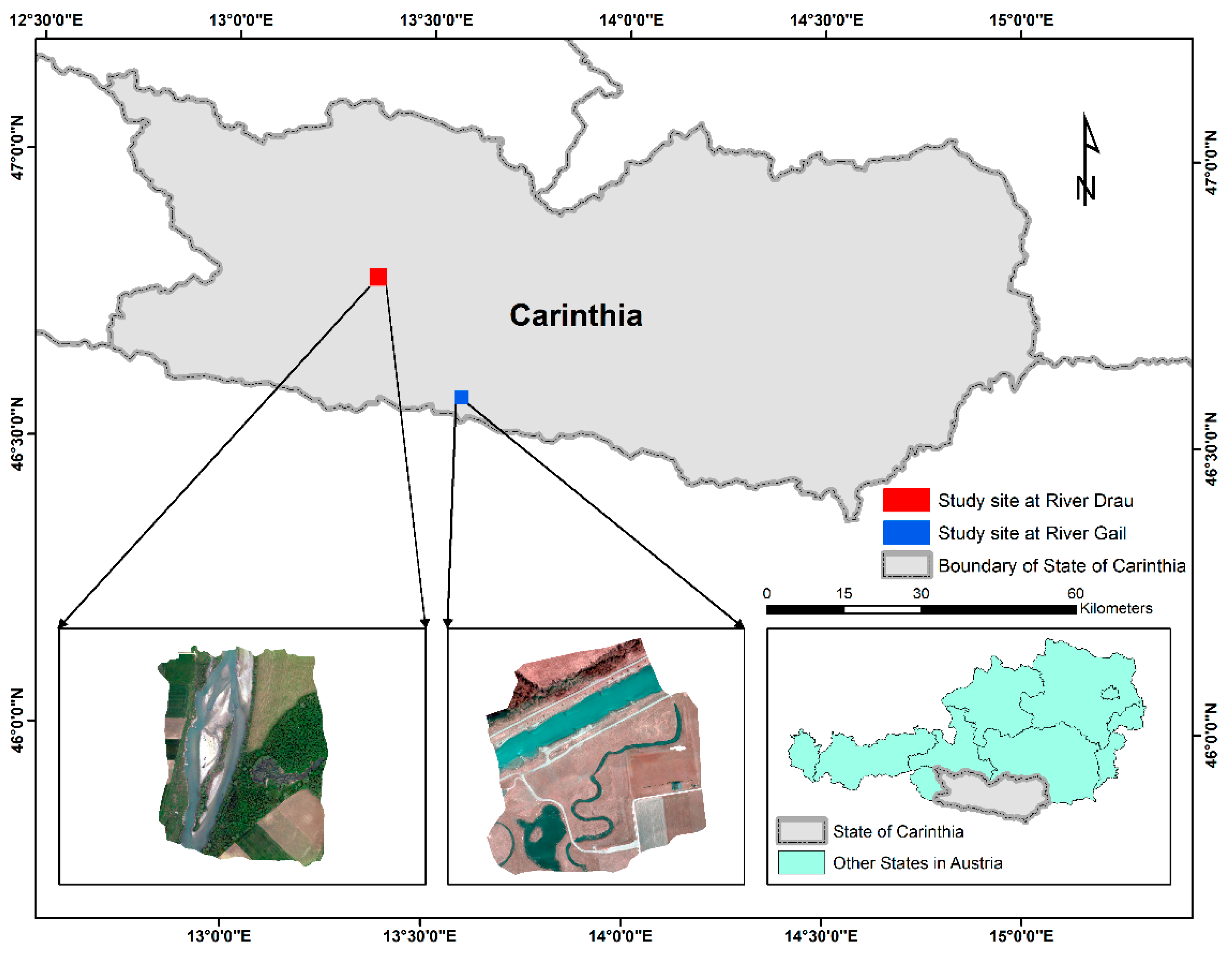
The two study areas are river reaches and their associated riparian zones of the Rivers Drau and Gail, respectively, located within the State of Carinthia, Austria (Figure 1). The reach of the River Drau analyzed is ~0.5 river km in length (where “river km” refers to the length of the river section of interest, measured along the river centerline, in this case in units of km), and it lies just east of Obergottesfeld, where the river valley has an approximately south–north orientation (as per the direction of river flow). Regarding the River Gail, the study reach analyzed has a length of ~0.35 river km, and it lies ~3 river km upstream of Feistritz, where the river has a southwest-to-northeast direction of flow. The study areas were determined by the coverage of the riparian/riverine zones that were captured by UAS-derived orthoimages and polygons from field-based mapping, described below. In recent years, both river reaches have been in various stages of restoration that were conducted as part of the Gail LIFE Nature Conservation project [
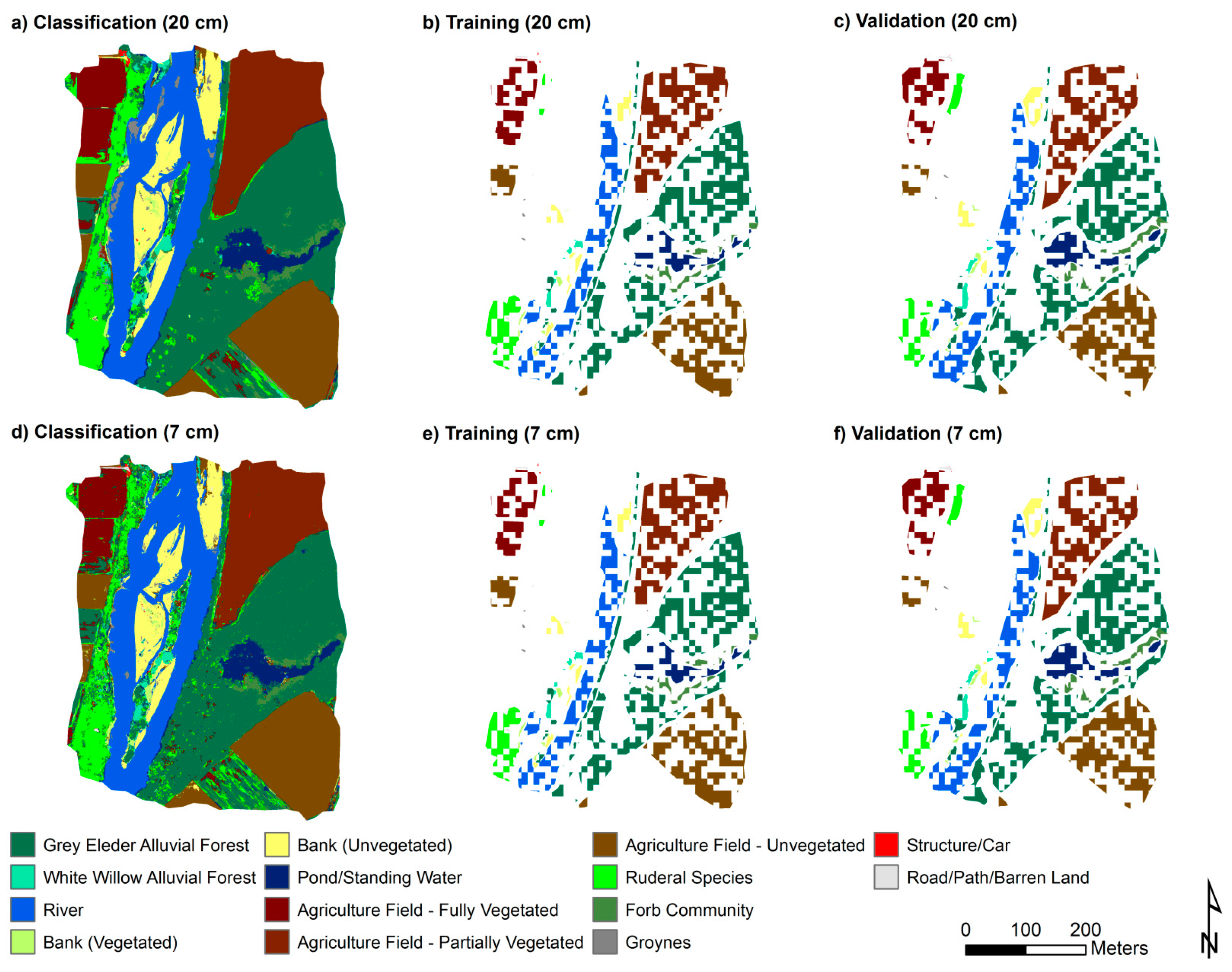
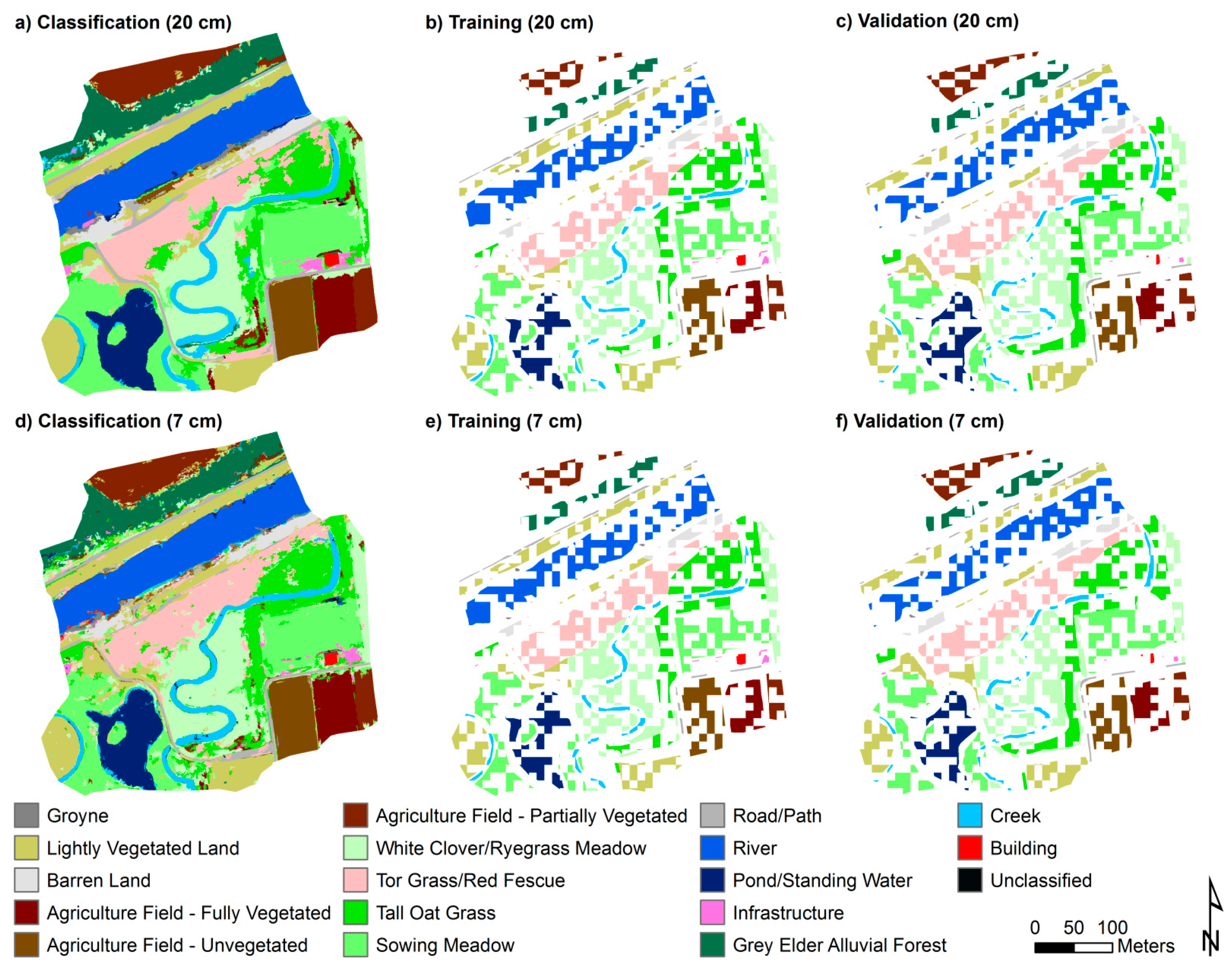
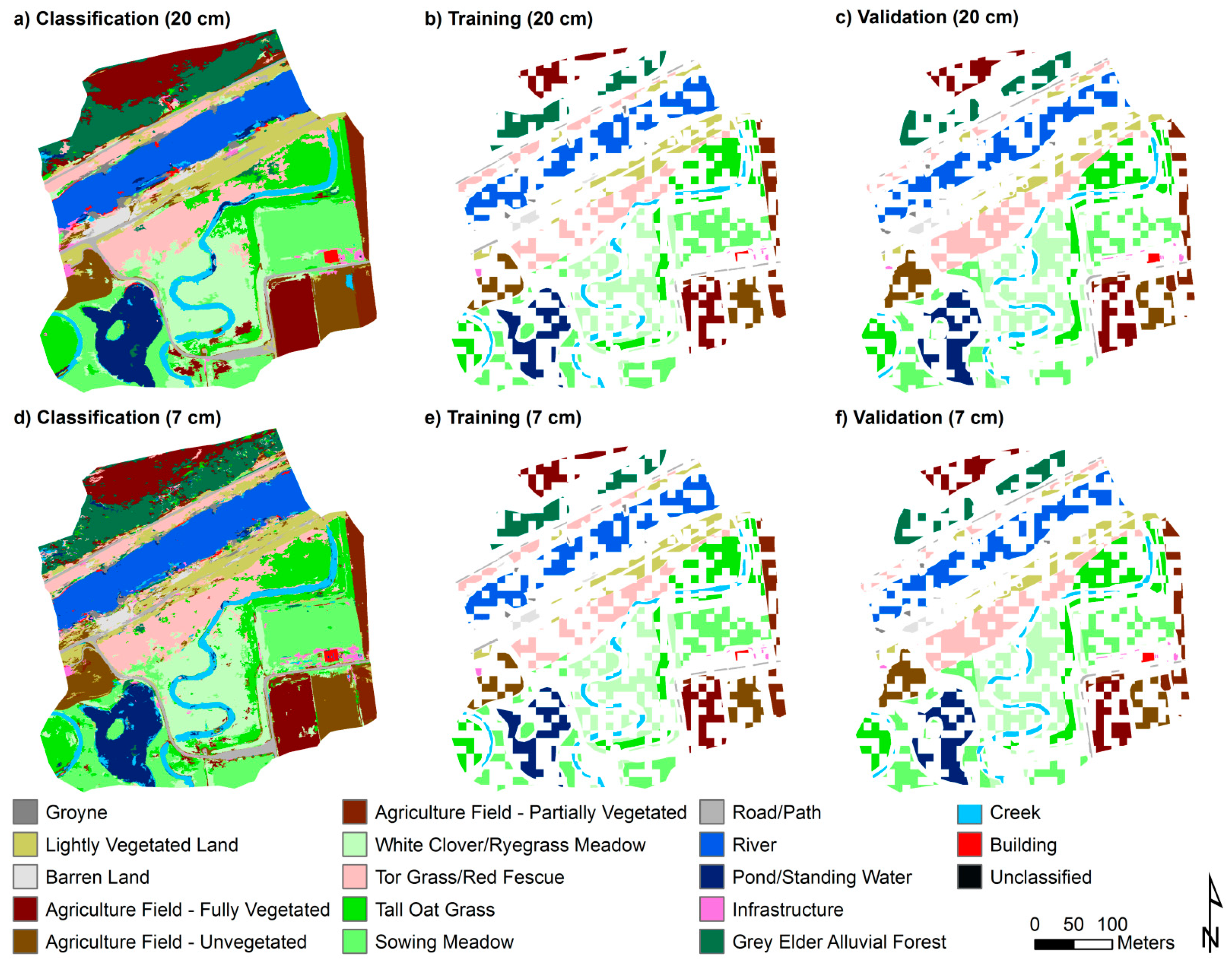
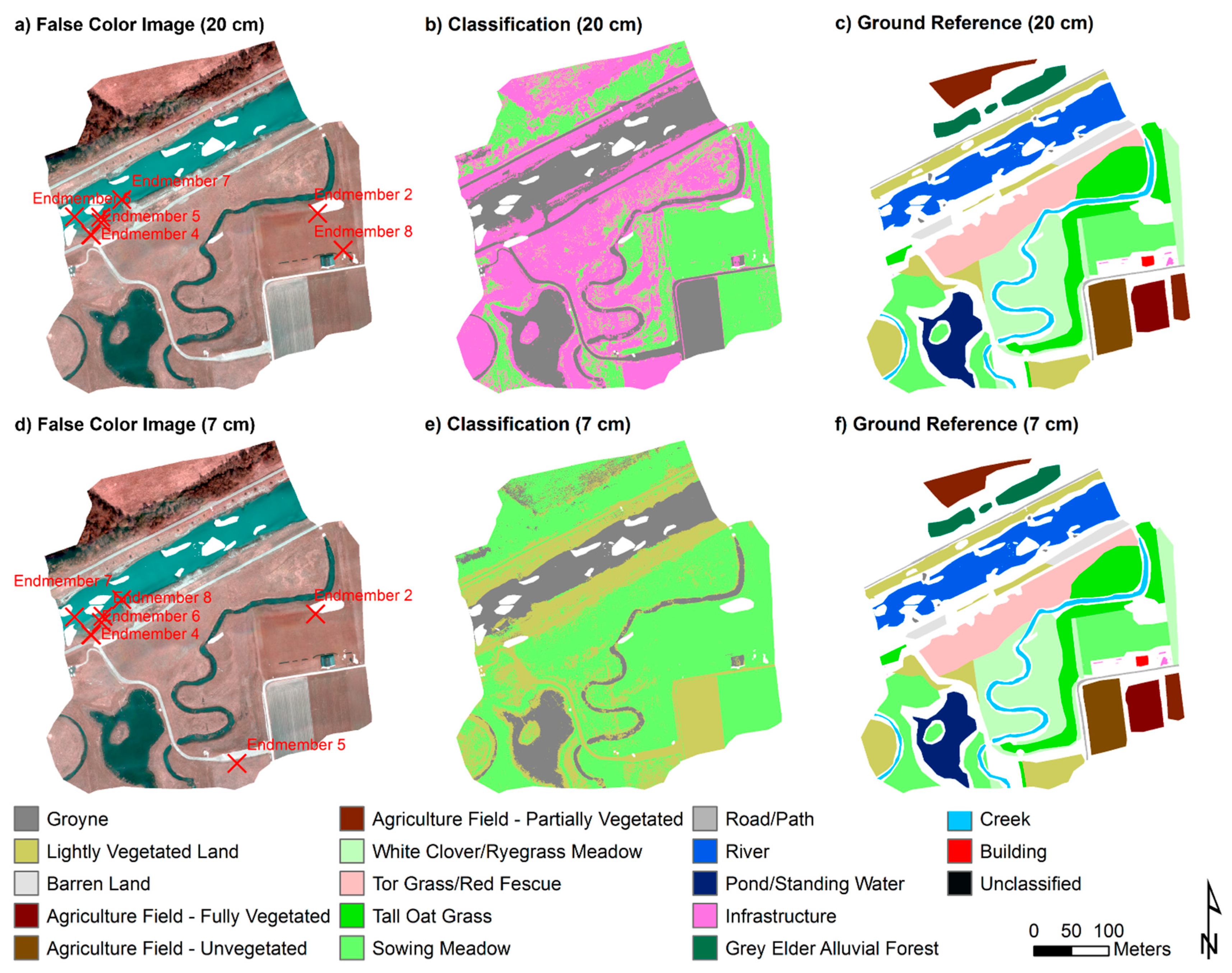
59]. The River Drau study area contains land cover types such as Grey Elder and White Willow alluvial forests, river water, vegetated and unvegetated banks, pond/standing water, and agricultural fields, with varying levels of vegetation cover. The River Gail study area includes the following land cover types, among others: Grey Elder alluvial forest, creek, river water, pond/standing water, sowing meadow and white clover/ryegrass meadow, and agricultural fields and other land, with varying levels of vegetation cover.

2.2. Data

Using a hyperspectral sensor mounted on a UAS platform flown by the Carinthia University of Applied Sciences (CUAS), Austria, we derive four (4) sets of narrow-band multispectral orthoimages. The narrow-band datasets consist of one (1) image for the River Drau, collected on 17 May 2016, and three (3) images for the River Gail that were collected on 11 April 2016, 22 June 2016, and 29 July 2016. Images used in developing these narrow-band datasets are all captured during a single UAS flight for each date, over the respective riparian areas. We mosaic and ortho-reference all collected imagery. We utilize a Rikola Ltd./VTT hyperspectral image sensor (CMV4000) (Oulu, Finland), based on Fabry–Perot Interferometer (FPI) technology, with a spectral range of 450–800 nm, though bands can be selected from the 400–950 nm range via long- and short-pass filters, and the minimum spectral resolution is 10 nm (FWHM). This lightweight sensor (<600 g) is designed for UAS mounting and applications.
Our main goal with the data collection part of this project is to perform an overall evaluation of a novel fixed-wing, UAS-based narrow-band, hyperspectral remote-sensing system. Here, for the first time, the Rikola hyperspectral sensor (Oulu, Finland) is fully integrated into the fixed-wing UAS platform (BRAMOR ppk, manufactured by the UAS company C-Astral (Ajdovščina, Slovenia)) (Figure S1; see Supplementary Materials), the high-precision autopilot (Lockheed Martin Kestrel Procerus Technologies, Vineyard, UT, USA), and the related flight mission planning software (GeoPilot–C-Astral, vers. 2.3.48.0-x86, Ajdovščina, Slovenia). BRAMOR ppk has a maximum take-off weight of 4.9 kg, electric propulsion, and a maximum flight duration of 3 h. BRAMOR ppk is launched by a catapult and landed by parachute, a safety mechanism for UAS operation. A Ground Control Station allows for monitoring of all relevant UAS parameters during flight. It is furthermore equipped with a survey-grade DGNSS system, which allows a positional correction of captured image coordinates by RINEX files, provided by the Austrian Positional Correction Service APOS. We have developed a semi-automatic process for hyperspectral mission planning, mission performance, and data post processing, yielding a complete workflow for hyperspectral imaging, starting with UAS mission planning. Based on the mission planning parameters in terms of flight altitude above ground level (AGL) (in our study, we generally employ a nominal flight AGL of 100 m) and overlap (70% front lap in the flight direction and 70% side lap between consecutive flight lines), the hyperspectral Rikola sensor (Oulu, Finland) is triggered by the Lockheed Martin Procerus Kestrel autopilot. For mission planning and post processing, we use C-Astral’s software GeoPilot (Ajdovščina, Slovenia) (Figure S2). For testing and evaluation purposes, we select the two (2) riparian/riverine test sites in Carinthia, Austria, and conduct multiple UAS missions with different settings regarding UAS flight parameters and narrow-band selection. Due to the mean flight speed of 16 m/s, a maximum number of 15 narrow bands can be captured during one (1) trigger event of the hyperspectral sensor. The rationale for the given band selections is to evaluate and test different band combinations as proof of concept. Furthermore, hyperspectral sensor integration was a challenge due to electromagnetic interferences from the Rikola sensor (Oulu, Finland), resulting in disturbance of the autopilot and UAS communication between the UAS and the Ground Control Station. This issue could be finally solved by additional shielding of the sensor.
Our hyperspectral UAS data mission preparation and data-processing protocol consists of four (4) main steps: (1) narrow-band selection and sensor pre-flight programing using Rikola’s internal software Hyperspectral Imager (Oulu, Finland); (2) converting raw data to radiance data cubes using Rikola’s internal software Hyperspectral Imager (Oulu, Finland); (3) applying Rikola DataProcessor software (Oulu, Finland) to convert the data cubes to reflectance factor images and generating individual GeoTiffs for each band as input for photogrammetric processing; and (4) hyperspectral photogrammetric processing of individual narrow-band images using Agisoft PhotoScan (St. Petersburg, Russia) in order to provide for each band an orthomosaic, digital surface model (DSM), and 3D point cloud.
The narrow-band image for the River Drau study site contains five (5) spectral channels/bands (with band centers at 457, 550, 670, 750, and 796 nm) at 7 cm spatial resolution and 32-bit radiometric resolution. Drau imagery is placed in a geographic WGS84 spatial reference (horizontal datum: WGS 1984; projection: transverse Mercator). Visual assessment of the narrow-band imagery indicates that the image has good band-to-band registration, and the river entails relatively clear water conditions that translate to only minor errors in the pixel values for the river water.
One narrow-band image for the River Gail entails 10 spectral bands (with band centers at 457, 492, 527, 562, 597, 632, 667, 703, 734, and 772 nm), and the other two River Gail narrow-band images contain 15 spectral bands (with band centers at 500, 510, 520, 530, 540, 550, 560, 570, 581, 590, 600, 670, 700, 750, and 797 nm). All narrow-band images acquired for this research have a nominal spatial resolution of 7 cm and high radiometric resolution; data are provided as 32-bit floating point values. River Gail imagery is placed in a geographic WGS84 spatial reference (horizontal datum: WGS 1984; projection: transverse Mercator). Visual assessment of the narrow-band imagery indicates that the 11 April 2016 and 22 June 2016 images have relatively erroneous band-to-band registration (particularly in areas in and around the river), whereas the 22 July 2016 image has better band-to-band registration (although not as good as the band-to-band registration for the Drau narrow-band image). River water was relatively turbid (especially for the two latter dates) during collection of the Gail narrow-band, yielding numerous errors in the pixel values over water, which can occur with the structure-from-motion-based mosaicking used.
Field mapping missions identify vegetation and other land cover types within particular portions of the respective riparian study areas where most of the river restoration efforts have occurred. This information is stored in polygon Esri© Shapefiles (Esri©, Redlands, California, USA) and contains data from mapping excursions conducted along the River Drau in 2015, and in 2014 for the River Gail. We extensively modify each of these datasets through manual digitization in order to match features that are visible within the orthoimagery, where the necessity for such modification is due to differences in geometry and other factors, such as seasonality (e.g., vegetation phenological and/or agricultural cycles). This results in each narrow-band image set having its own corresponding land cover dataset that was derived using the 2014 or 2015 shapefiles. Table 1 and Table 2 show the land cover classes that were ultimately used in our classifications. Some of the narrow-band classes in Table 1 and Table 2 are from the original land cover shapefiles for 2014 and 2015, whereas we determine others visually, via on-screen image interpretation. We use these data in classifier training and validation of our image classifications. We use all reference data to validate the endmember-based classifications (since the endmember-based classifications do not require training data), and for the GEOBIA classifications, we use 51% of the reference data for training and 49% of the data for validation. We divide the original polygons into smaller features by dividing them using a fishnet. We use a stratified random sample to select 51% of the reference data for training and the remaining 49% of reference data for validation. We chose those percentages for the training and validation data because this is an approach used in the calibration and validation of empirical models that makes use of all the available reference data, e.g., [60,61]. Those percentages also limit the data included in the model calibration, given the computational intensity of the classifier. The slightly larger fraction of reference data being dedicated for calibration follows the practice of using at least half of the available reference data for calibration, while also allowing a comparable validation dataset with a variance similar to that of the calibration data to be developed. We then perform a merging scheme, where rooks case neighbors are merged to have features of the training and validation data of variable size. Our initial set of segments is joined with the training data using a majority zonal statistics operator.

2.3. Data Pre-Processing

The positional accuracy of the captured individual image coordinates is improved by utilizing RINEX DGNSS correction data via GeoPilot (Ajdovščina, Slovenia). Furthermore, VHR broad-band RGB orthomosaics, captured during a temporally close prior UAS mission (via a Sony Alpha 6000 camera, Tokyo, Japan) and georeferenced by using DGNSS ground control points in the photogrammetric processing with Agisoft PhotoScan (St. Petersburg, Russia), are also used for co-registration purposes. All data are projected to the UTM spatial reference system (zone 33; horizontal datum: WGS 1984; projection: transverse Mercator). Using visual overlay analysis, we determine that the narrow- and broad-band imagery do not align geometrically and that the broad-band imagery has more geometric agreement with standard orthophoto products generated by the Austrian government than the original narrow-band imagery. Thus, we register the narrow-band imagery to the broad-band imagery. For this further correction, each narrow-band image is warped using a third-order polynomial, with root mean square error (RMSE) values of 6 (18 tie-points), 36 (18 tie-points), 40 (18 tie-points), and 4 cm (19 tie-points) for the 17 May 2016 (Drau), 11 April 2016 (Gail), 22 June 2016 (Gail), and 29 July 2016 (Gail) images, respectively.
We atmospherically correct the UAS-based images, as we consider image classifications across multiple dates. The hyperspectral camera acquired data for the narrow-band images in units of radiance (mWm−2sr−1nm−1), and we use the QUick Atmospheric Correction (QUAC) algorithm [62] to atmospherically correct each image, converting the radiance values for the pixels to surface reflectance. QUAC is considered to be more of an approximate atmospheric-correction method relative to radiative transfer-modeling approaches; image-specific information sufficient to perform such a physically-based atmospheric correction (e.g., via FLAASH [63]) is unavailable.
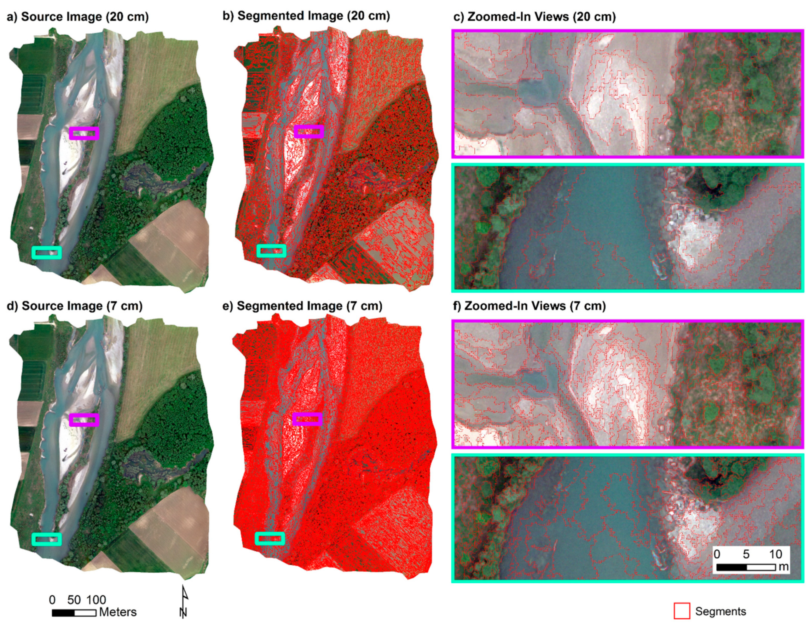
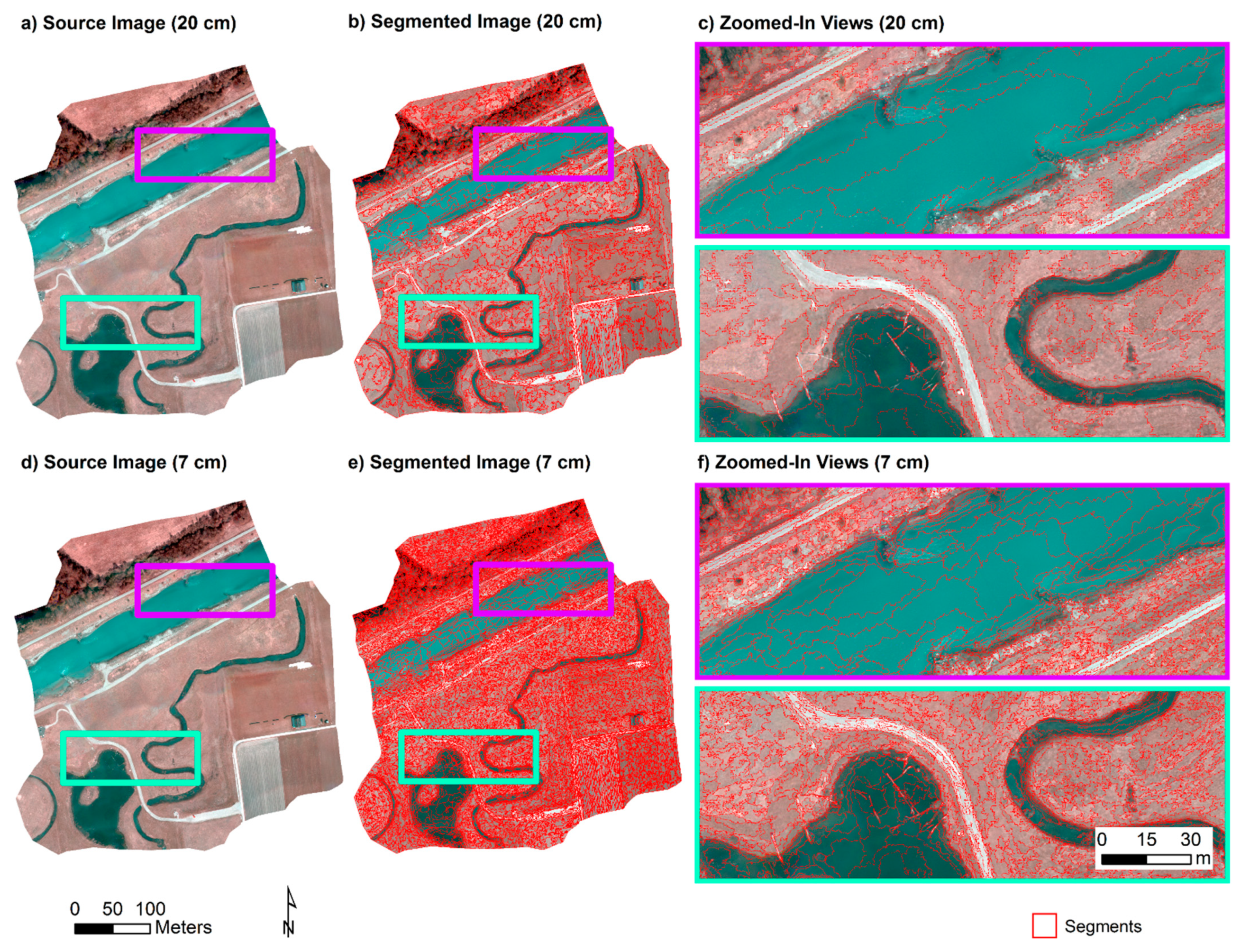
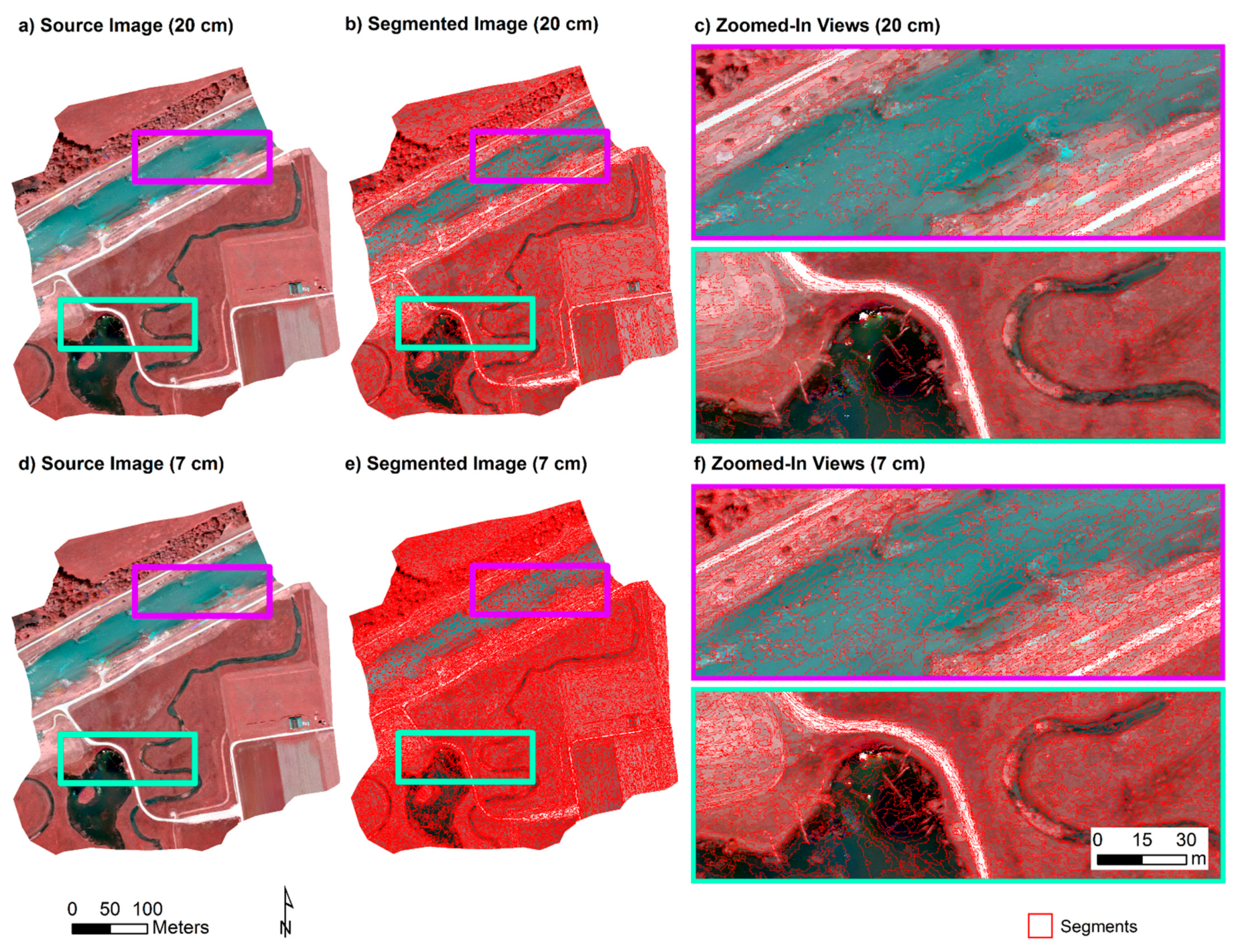
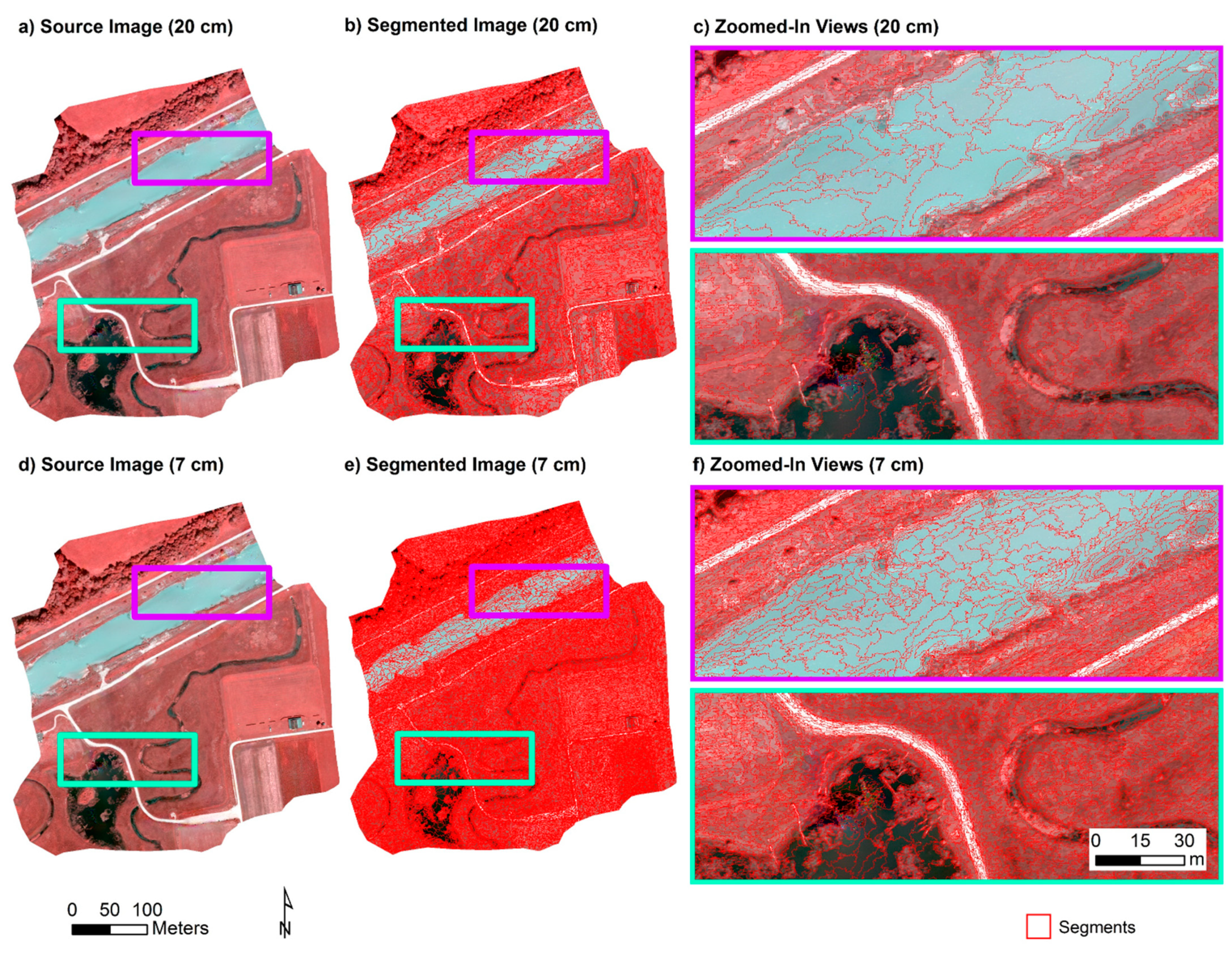
In order to maintain a consistent geographic area for each riverine/riparian area within our areas of interest, we clip all narrow- and broad-band images (noted above) to the same extent and shape for each of our study reaches. We determine the final study area by overlaying all narrow-band and broad-band imagery and manually delineating a polygon that captures all the necessary data while minimizing band alignment issues along the edges of the study areas. The finalized images that serve as the basis for our object- and endmember-based analyses are shown in Figure 2, Figure 3, Figure 4 and Figure 5. Moreover, endmember-based analysis can be sensitive to extreme/erroneous pixel values that can arise due to sun glint over water and errors in the image stitching from the structure-from-motion mosaicking process. Thus, prior to the endmember-based analysis, we mask out parts of the study area with large amounts of extreme/erroneous pixel values.
To assess the effect of pixel size on classification accuracy, in addition to the original 7 cm spatial resolution image data, we resample all of our narrow-band imagery to a coarser pixel size of 20 cm. We choose this value because it is the same pixel size as that of other multispectral (blue, green, red) aerial orthoimages of our riparian study sites collected under the auspices of the Carinthian government (Austria) for mapping purposes. In the present study, all classification experiments conducted on the 7 cm spatial resolution images are repeated on the 20 cm pixel size images. This allows us to infer how comparable our CUAS data are with Carinthian governmental data.

2.4. Object-Based Land Cover Classification of Narrow-Band Imagery

We perform segmentation/feature-extraction and object-based classification (i.e., GEOBIA) [36,37] on the narrow-band images using eCognition® Developer software (vers. 9; [64,65]), which allows objects/segments to be delineated and used to classify geospatial datasets. We classify all narrow-band images for both study sites using the same workflow (or rule set). The rule set involves five (5) general steps, described as follows:
The first (1) step involves segmenting the narrow-band image. We use Multiresolution Segmentation to segment the input image. This is a type of bottom-up segmentation, in that it starts by creating objects of a single pixel, and it grows the size of objects by merging neighboring objects until some homogeneity criterion has been met [37,64]. There are three parameters that affect the homogeneity criterion, and they include scale, shape, and compactness. Scale affects the size of the objects, with higher scale values generating larger objects. In segmenting the narrow-band imagery, we use a scale value of 200, enabling the delineation of forest stands. Shape determines how much the geometry of the object influences the homogeneity criterion when compared to the variability in spectral values within each object. Here, we use the default shape value of 0.1, and this indicates that color (i.e., spectral values) has a much higher weighting in determining the homogeneity criterion because the shape and color parameters need to sum to 1. Thus, color has a weight of 0.9. Compactness influences how the object shape is compared with regard to some idealized geometry. In this study, we employ the default compactness parameter value of 0.5, which indicates that we have no preference with regard to how compact or smooth the objects need to be when computing the homogeneity criterion. Narrow-band images that we subjected to Multiresolution Segmentation are shown in Figure 2, Figure 3, Figure 4 and Figure 5.
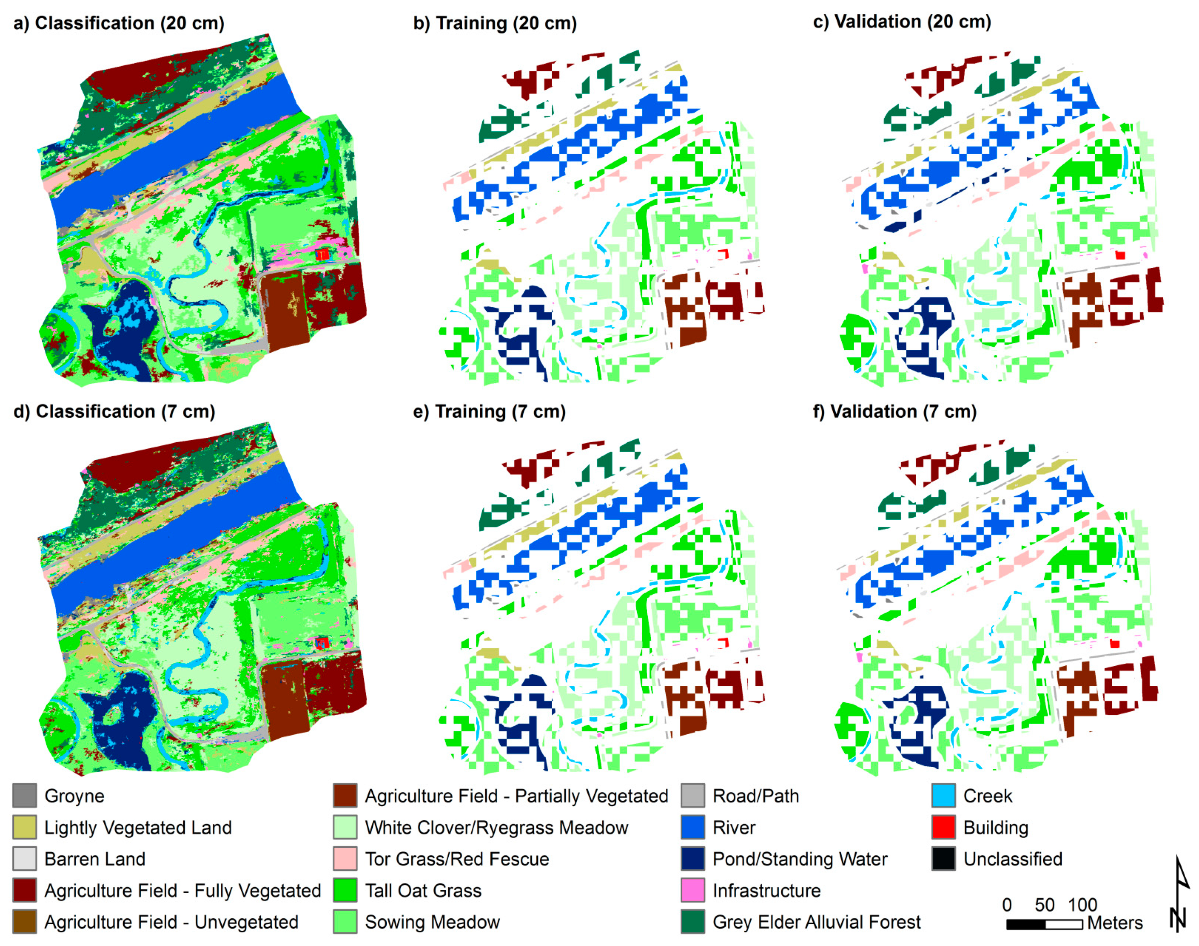
The second (2) step involves assigning a class to segments that overlap features of some reference dataset. We use the reference data compiled for training (see Section 2.2) in order to assign the narrow-band imagery classes in Table 1 and Table 2. Segments that intersected a feature within the training dataset are assigned that particular feature’s narrow-band imagery class. If more than one feature in the training dataset intersected a segment, then the feature that occupied the most space within the segment would be the class assigned to the segment. The training areas used to assign classes for the narrow-band imagery are shown in Figure 6, Figure 7, Figure 8 and Figure 9.
The third (3) step involves converting the segments that were assigned a class in Step 2 into training areas. Built-in functionality within eCognition® is used to accomplish the conversion in a simple manner.
The fourth (4) step is to configure the feature space of the Nearest Neighbor classifier that will be used to classify the image objects. Configuring the feature space involves specifying the object properties that will be used as the basis for classification. The object properties that we used in classifying the narrow-band imagery are given in Table 3. Regarding some of the object properties noted in Table 3, for the 17 May Drau image, we compute the Normalized Difference Vegetation Index (NDVI) [66,67] and the Normalized Difference Water Index (NDWI) [67] via the following: NDVI = (796 nm − 670 nm)/(796 nm + 670 nm); and NDWI = (550 nm − 796 nm)/(550 nm + 796 nm), respectively, where values are the band-center wavelength for each band. For the 11 April Gail image, the bands used to calculate NDVI and NDWI, respectively, are indicated as follows: NDVI = (772 nm − 667 nm)/(772 nm + 667 nm); and NDWI = (562 nm − 772 nm)/(562 nm + 772 nm). For the 22 June Gail and 29 July Gail images, the bands used to calculate NDVI and NDWI, respectively, are indicated as follows: NDVI = (797 nm − 670 nm)/(797 nm + 670 nm); and NDWI = (550 nm − 797 nm)/(550 nm + 797 nm).
The fifth (5) and final step involves applying the configured Nearest Neighbor classifier to the image objects. This algorithm determines how close an object is to a given feature space for a particular class (as determined by the configuration) by using a membership function [64]. The more similar an object is to a particular feature space, the higher the membership that will be assigned. Parameters of the Nearest Neighbor classification that need to be specified are the classes that will be included in the classification and the slope of the membership function. All narrow-band classes listed in Table 1 and Table 2 are included in the classification. We use the default membership function slope of 0.2, which allows a more subtle gradation in the assignment of feature space membership.

2.5. Endmember-Based Land Cover Classification of Narrow-Band Imagery

Endmember extraction algorithms (EEAs) and endmember-based classifications are applied to each set of narrow-band imagery. As discussed in 
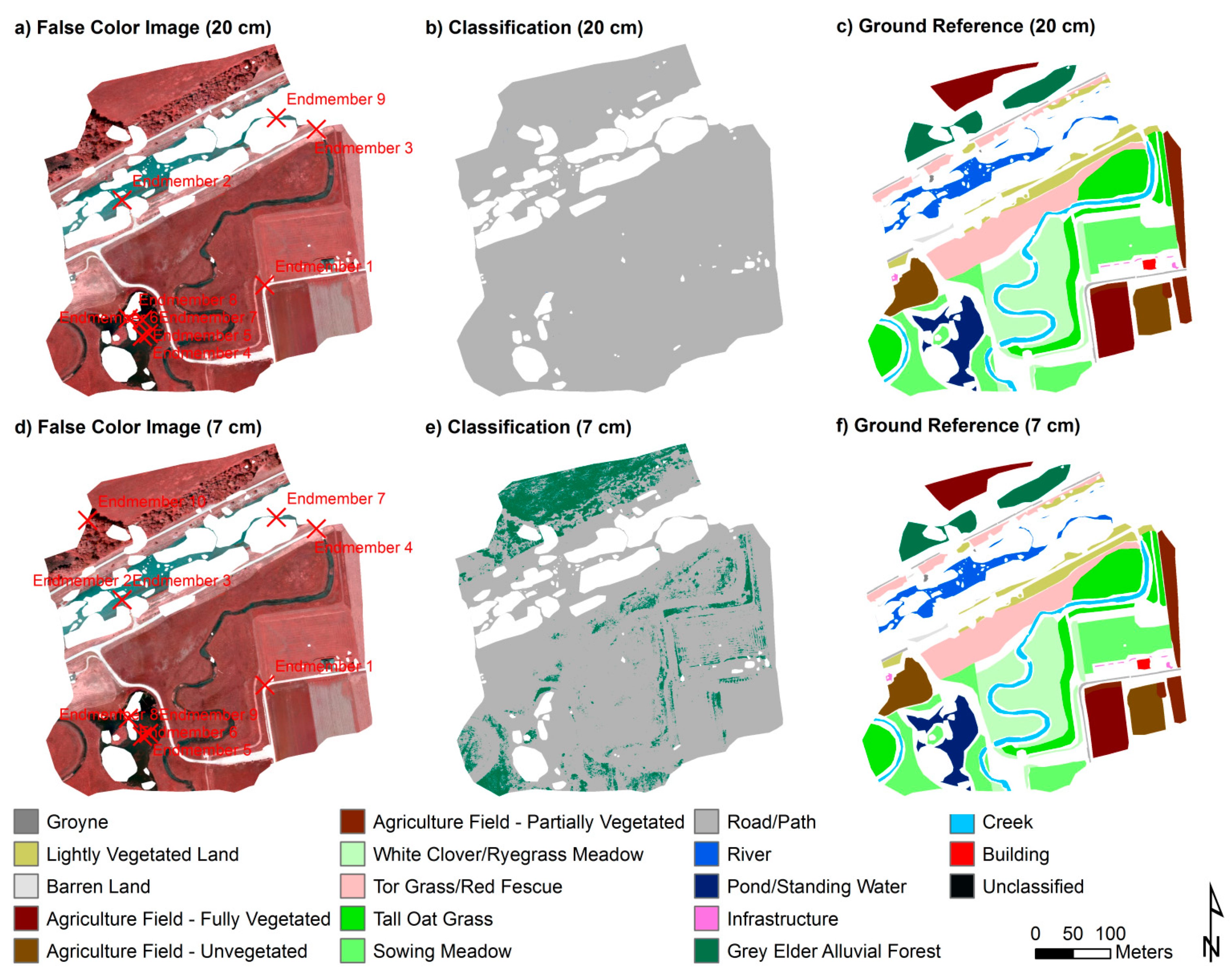
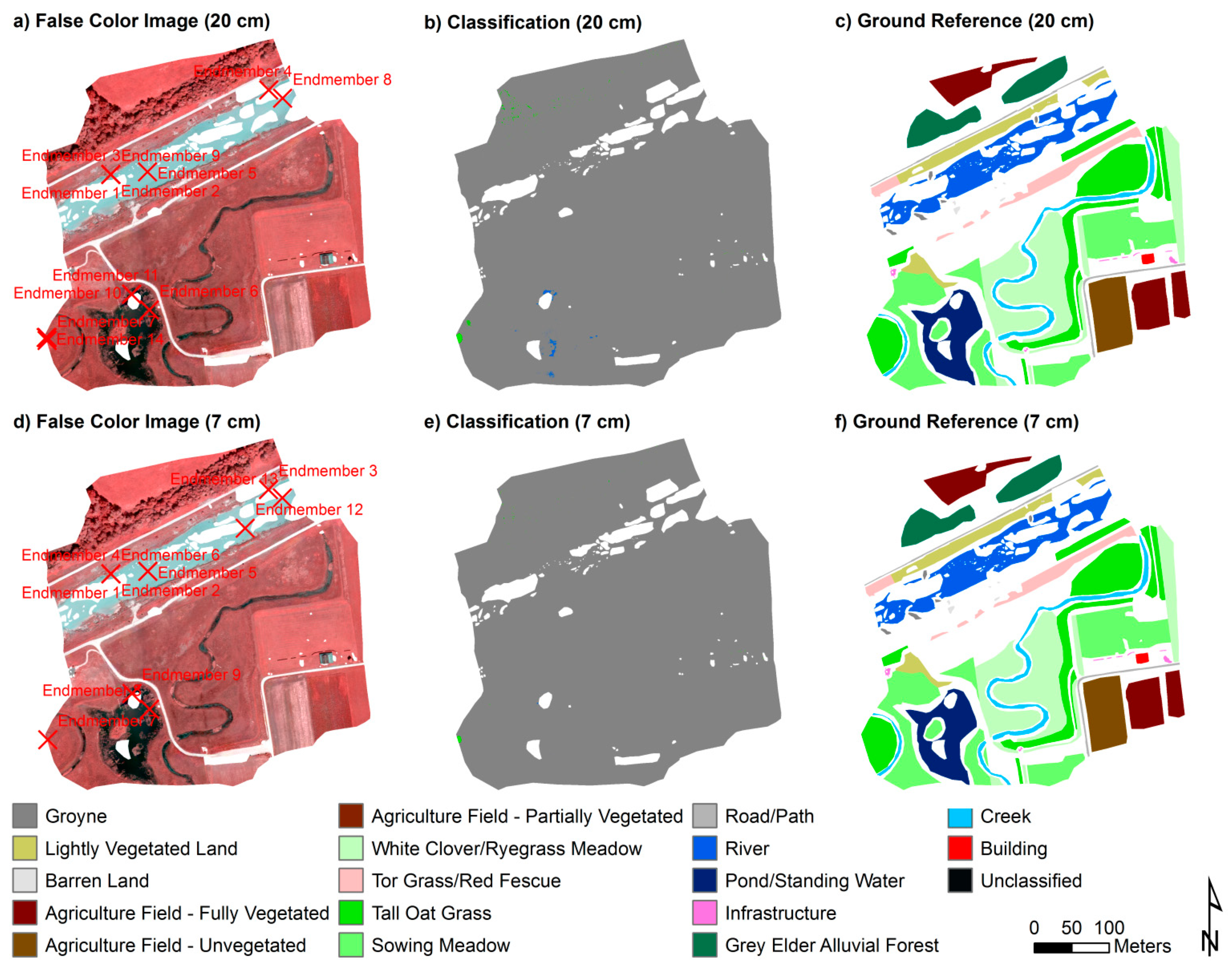
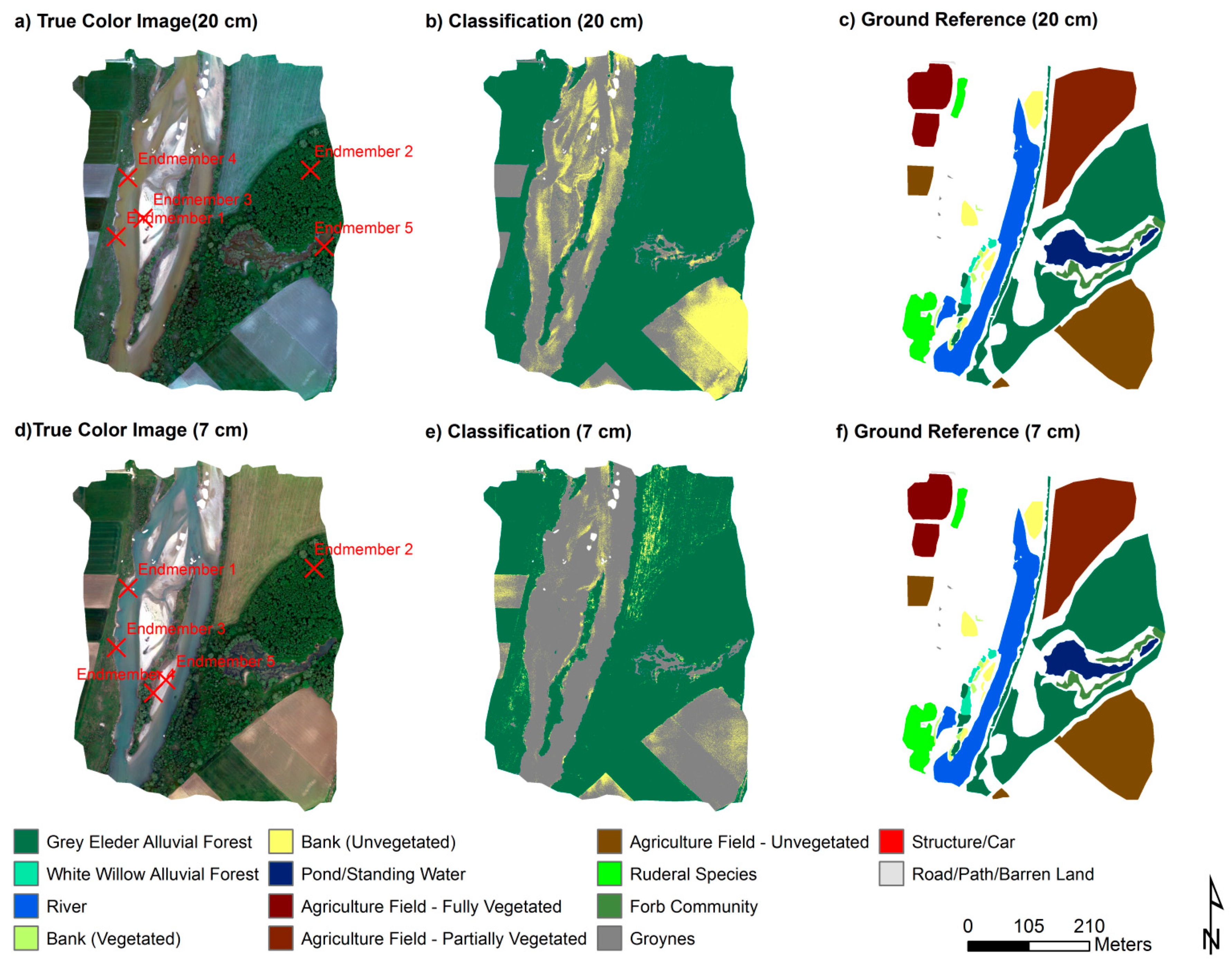
Section 2.2, EEAs can be sensitive to extreme/erroneous pixel values, and we mask out these areas within each narrow-band image. The narrow-band images subjected to endmember-based processing are shown in Figure 10, Figure 11, Figure 12 and Figure 13.
Our endmember-based classification involves three (3) general steps. First (1), the dimensionality, or discrete number of information signals, within the multi-band data is estimated. Given that we are analyzing aerial images acquired over landscapes, it is commonly assumed that the dominant signals in the data correspond to land cover and other features within the images. We employ three well-known algorithms for estimating dimensionality of imagery, and they include Harsanyi–Ferrand–Chang (HFC) [68], noise-whitened HFC (NWFC) [69], and the hyperspectral signal identification by minimum error (HySime) algorithm [70]. We apply each dimensionality estimation algorithm to each image mosaic, and we vary the value for the probability of failure (PoF) for HFC and NWHFC that is used to stochastically test whether the number of signals is statistically significant. The number of estimated dimensions for each algorithm and PoF specification are given in Table 4 (20 cm pixel size) and Table 5 (7 cm pixel size).
The value of the maximum number of estimated signals is used as an input to the endmember-extraction step based on use of the Sequential Maximum Angle Convex Cone (SMACC) EEA [71,72], available within the ENVI® digital image processing environment. The number of endmembers extracted for each image is listed in Table 6. SMACC identifies the “pure pixels” that are used to develop the endmember spectra, and these locations are shown in Figure 10, Figure 11, Figure 12 and Figure 13. Outputs from SMACC include the endmember spectra and respective fractional-abundance maps for the respective classes represented by their corresponding endmembers, and these data are used to produce hard/crisp endmember-based classifications.
In particular, we employ the SMACC-extracted endmembers as input for the Spectral Angle Mapper (SAM) [73] algorithm within ENVI® (vers. 5.4) in order to generate hard/crisp classifications. For the SAM hard classifications, we use a maximum angle threshold value of 0.8 radians, so that all pixels in the input image are classified. Once the classifications are generated, we use the pure pixels (Figure 10, Figure 11, Figure 12 and Figure 13) employed in developing the endmember spectra and the angle maps generated by SAM for each endmember in order to label each endmember (i.e., we associate each endmember with its corresponding narrow-band image land-cover class name) (Table 1 and Table 2). That is, we incorporate the field data in the endmember-labeling process.

2.6. Accuracy Assessment of Land Cover Classifications

We assess the accuracy of our narrow-band object-based classifications using the 49% of reference features that were not used in classifier training (validation in Figure 6, Figure 7, Figure 8 and Figure 9). All reference data (Figure 10, Figure 11, Figure 12 and Figure 13) are used in the accuracy assessment of endmember-based SAM classifications. We use a simple pixel-based overlay analysis between the classified imagery and validation reference data. More specifically, we accomplish the accuracy assessment of the classified images by conducting a cross tabulation between the classified image and the validation reference data using an overlay approach. We utilize the cross tabulation to develop error matrices that we further process to generate statistics of the classification accuracy [74,75].

3. Results

3.1. Object-Based Land Cover Classification of Narrow-Band Imagery

Figure 6, Figure 7, Figure 8 and Figure 9 show the land cover classifications produced using the described object-based analysis. All classes included as part of the classifier training appear in the dataset. Tables S1–S3 (see Supplementary Materials) indicate the amount of spatial coverage associated with each class, by classification method and by pixel size experiment. With the exception of the 29 July 2016, which is quite heterogeneous/speckled (and possibly noisy), with numerous, small land cover patches scattered throughout the study area, all the other narrow-band object-based classifications generally entail more homogenous areas. Fronts of major land cover transitions are the locations within the respective images where the classifications tend to be the most spatially heterogeneous (and possibly noisy).

3.2. Endmember-Based Land Cover Classification of Narrow-Band Imagery

Figure 10, Figure 11, Figure 12 and Figure 13 show the land cover classifications that were produced using endmember-based analysis. Table S4 (see Supplementary Materials) lists the amount of coverage that occurs for each class. Only a few of the classes in the reference dataset were mapped. The extent of individual classes is very generalized, with very large patches of the classes that were mapped. It appears that SMACC only extracted the general signals for features such as vegetation and barren land classes (e.g., groynes and banks). Moreover, it seems that SMACC is only able to detect/identify the higher-reflectivity features within these images, as no water classes were mapped via the subsequent SAM classification.

3.3. Accuracy Assessment of Land Cover Classifications

Accuracy assessments are conducted for each of the narrow-band image classifications, and the overall accuracies for each method, for each of the study areas, by image date and by pixel size, are shown in Table 7. All of the endmember-based classifications are of very low thematic accuracy, with the exception of the classifications for the River Drau study area. For the object-based classifications, with the exception of the River Gail study area classifications for 29 July 2016, all of the classifications have overall accuracies of >85%. We also construct error matrices, yielding the error associated with each class, and they are shown in Tables S5–S19 (see Supplementary Materials).

4. Discussion and Conclusions

Various factors likely affect the accuracies of the object- and endmember-based classifications. The relatively high overall classification accuracies for the object-based classifications generated in this study may follow from the fact that we utilize a relatively large number of samples for training in our workflow/rule set. With regard to the poor classification accuracies from the endmember-based approach, this is likely largely attributable to the very small pixel sizes, as well as to the relatively large number of classes used for these classification systems, in conjunction with the relatively small number of bands available with the UAS-derived orthoimages, even though their bandwidths are narrow. Lower endmember-based classification accuracies are, in fact, obtained for the River Gail study site (Table 7), even though a higher number of spectral bands are employed for those classifications (10–15 spectral bands), compared with the River Drau classification (5 spectral bands). Regardless, the overall results suggest that endmember-based classification of data with very high-spatial resolutions (VHR) should likely only be performed when more spectral bands are available. There are often many more endmembers than materials in a given image; for a given material, it is possible for exemplars to be present in an image that correspond to extremes in the state, or condition, of that material (e.g., due to shadowing/solar illumination variability, weathering, pigmentation). This possibly yields a large number of endmembers for a single material type [71]. Such a situation is likely to be accentuated by the use of VHR image data, with the associated possibility for larger numbers of pure pixels for a given class, relative to coarser pixel size data. Additionally, importantly, regarding SAM, the endmember-based classifier that we employ here, we use a single, constant maximum angle threshold value. That value may not be optimal, however, and is a factor that may significantly affect image classification accuracy. In addition, the overall wavelength ranges associated with the bands used for each riparian study site are similar. The majority of the bands we utilize are located in the visible wavelength range; the addition of more bands in other spectral regions (e.g., the near-infrared (NIR) and, if available, depending on the sensor type, the mid-infrared (MIR) regions) is expected to increase classification accuracy, particularly for vegetation, and for land–water discrimination [76,77]. Furthermore, the classification systems between the two study sites vary, so that is likely a factor in the classification accuracies attained, for both the endmember-based and object-based classifications. More work involving the merging of some classes may increase classification accuracy, as a smaller number of classes into which pixels/objects are classified typically translates into higher classification accuracies.
Poor band-to-band alignment for some of the narrow-band images likely also contributes to errors in both types of classifications, though the endmember-based classifications may be more adversely affected by this type of error, which affects pixel spectra. It is expected that river water misclassifications, such as those in Figure 7 and Figure 8, would be minimized if the narrow-band datasets had better band-to-band alignment. We only employ a small set of pixel- and object-based ancillary input data in our land cover classifications, though the use of other types of ancillary data may also increase classification accuracy. For example, explicit texture measures could increase riparian and water image classification accuracy. Texture information for forest and non-forest vegetation, for instance, that derives from a variety of texture metrics would be quite different, and hence, would likely aid in class discrimination in a riparian environment [76,77]. It is also possible that the Nearest Neighbor classifier within eCognition® may not optimally exploit the spectral and shape information of the delineated image objects. Thus, a more complex classification algorithm, such as Support Vector Machines (SVMs) [78,79] or an artificial neural network (ANN)-based approach [34,35], could potentially perform more accurately.
In addition, image objects/segments are also processed, generated, and assessed over different scales. The size of pixels and objects/segments can potentially affect the image classification accuracy, but we do not observe any consistent improvements in overall accuracy at any scale. In this study, only two scales/pixel sizes are utilized; the results seem to be more sensitive to the band-to-band alignment and erroneous/extreme pixel values, rather than pixel size, given the pixel sizes evaluated. Further research is needed in order to determine whether other processing scales or classification parameterization schemes can improve the accuracy of results. Additionally, there does not seem to be a clear relationship between image acquisition date and classification accuracy for these study sites, though we note that the lowest accuracies are generally observed for the 29 July 2016 image date, across classifiers.
We also posit that some of the apparent classification errors, as given in the classification accuracy assessments, may also be a consequence of inaccuracy in the ground reference data, rather than of the image classifications themselves. With respect to possible problems with the accuracy/level of detail of the reference/field land cover dataset, thematic inaccuracies in the field data are possible, where such potential categorical errors could be a function of the field methodology used and/or other factors. Additionally, some marked within field reference polygon class heterogeneity may not be represented, in which case RS classifications could be more accurate than the reference data in some cases/areas (perhaps even more so with the endmember-based classifications). We also observe some spatial errors in the delineations of certain features in the polygonal field data (Esri© Shapefiles); as described in Section 2.2, some geometric inaccuracies may exist with the ground reference data. Furthermore, temporal disjunctions between the time at which the ground reference data were collected and the date of UAS image acquisition could also constitute a significant factor in the reported image classification errors. The temporal offset and the associated landscape changes between the field and image datasets is particularly pronounced with the River Gail reach of interest. These issues resulted in our extensively modifying the reference data using visual/manual image interpretation, and errors in our interpretations may have also influenced overall accuracies.
This research quantitatively evaluates the utility of the object-based algorithms within the eCognition® environment when operating on very-high-spatial-resolution (VHR) narrow-band UAS-based image data, yielding relatively high classification accuracy, where most classifications attain overall accuracies of >85%, across the study sites and image acquisition dates. For comparison, we also test the efficacy with which endmember-based analysis could be used for classifying VHR narrow-band images in riparian environments, and all such classifications entail very low accuracy. Somewhat similar classification accuracies of endmember-based methods have been obtained previously, including Filippi et al. [80]; based on a standard image dataset, several endmember-based classification methods were compared, where most overall classification accuracies varied between 47% and 62%, but where some had accuracies of ~24% and ~1.5%, respectively. Those results, though, were derived from remote-sensor image data that were not as high-spatial-resolution as those in our present study (pixel size = 20 m). Additionally, in that study, as in the present research, constant rule-classifier thresholds for endmember-mapping algorithms were used, which may contribute to such lower classification accuracies. Regarding previous research involving direct comparison of endmember-based and segmentation/object-based results, Mishra and Crews [58] estimated fractional land cover in a semi-arid environment using MESMA and hierarchical OBIA, respectively, applied to GeoEye-1 imagery (pixel size = 2 m). Their results indicated that MESMA yielded more accurate fractional cover estimates, though in some trials OBIA and MESMA-derived estimates were similar. (Note that because of the limited field-transect data collected in [58], MESMA-derived fractions were used to validate OBIA results.) Various aspects of that study [58] and the present research differ, however, including the spatial resolution/pixel size; thus, the results between the studies are, of course, not directly comparable. In any case, in the present study, we conclude that a greater number of spectral bands is likely necessary in order for the endmember-based methodology to produce more viable classifications in this context, with such pixel sizes and algorithms employed. As noted, the effects of differing pixel size—of those tested—are generally not large in most cases and are not consistent. It is possible that coarser pixel sizes (coarser than those tested here) may actually enhance endmember-based classification accuracies (perhaps up to some threshold pixel size), as may other endmember-based classification approaches that can better handle VHR image data. Regarding EEAs, there may actually be a large number of endmembers per class when using VHR data (e.g., multiple endmembers associated with varying leaf angle distributions and/or leaf/canopy biophysical, or health, characteristics within a forest class, etc.); conventional EEAs may not be able to handle this, particularly when a limited number of bands are employed.
To facilitate broad relevance of this study to the remote-sensing, forestry, riparian, and other research communities, as well as riparian/floodplain managers, we investigate commonly used/widely available EEA/endmember-mapping and GEOBIA algorithms, within the ENVI® and eCognition® software environments, respectively. In this study, we find that object-based classification provides for an avenue for effective riparian forest/zone monitoring and management. However, with further research, endmember-based classification may also play an important role in this domain.
Regarding future research, further work pertaining to the object-based classification approach may involve performing GEOBIA experiments based on smaller training sets (i.e., evaluating the effect of training set size on classification accuracy). Object-based classification accuracy assessments in this context could also be investigated. Future work could specifically involve the use of geometric and non-geometric indices to compare segmentations, and classification results can be compared via additional measures (e.g., multi-class F-scoreM) [81]. Additional research involving endmember-based classification of VHR narrow-band images for mapping riparian forests and other land covers should involve the use of truly hyperspectral data, which entails a larger number of bands. Additionally, as noted, there are often many more endmembers than material types in an image, and this may be even more so the case when EEAs are operating on VHR images. In [82], for example, endmember variability was integrated into spectral mixture analysis via the representation of each endmember by an endmember bundle, or set of spectra; such an approach could potentially address this general issue. This condition/scenario also suggests that future research may include experimentation with other methods for determining the number of unique signal sources/endmembers, as well as more advanced EEAs, including: (a) those that are not limited by the n + 1 constraint on the number of endmembers extracted, where n = the number of bands, such as SVM-BEE, proposed in [18]; and/or (b) EEAs that incorporate spatial information (e.g., the spatial/spectral AMEE endmember algorithm [83]). Regarding endmember-based classification, as SAM is employed in the present research, future research also includes sensitivity analysis of the effect of the SAM maximum angle threshold value (in radians) on classification accuracy, in order to optimize that value. Furthermore, since we only evaluate the efficacy of SAM in this study with respect to endmember-based classifiers, future extensions of this line of research should include testing of other endmember-mapping algorithms and performing sensitivity analyses of their parameter values. Additionally, for whatever EEA/endmember-mapping algorithms are considered in future research, sensitivity experiments should be conducted across a broader range of pixel sizes, particularly considering coarser pixel sizes, in order to ascertain an optimal pixel size for the scenario(s) evaluated, or otherwise to determine the effect of pixel size in this regard in more detail.

Supplementary Materials

The following supporting information can be downloaded at: https://www.mdpi.com/article/10.3390/land11020246/s1, Figure S1: View of the fixed-wing UAS platform deployed in this study (BRAMOR ppk (C-Astral, Ajdovščina, Slovenia), where the Rikola Ltd./VTT hyperspectral image sensor (CMV4000) (Oulu, Finland) is fully integrated into the platform. Figure S2: Example of a UAS mission plan for the River Gail study area, Austria, within the C-Astral GeoPilot software (Ajdovščina, Slovenia). Table S1: Spatial coverage (in units of ha) of land cover types from object-based and endmember-based classifications for the River Drau (17 May 2016) imagery. Table S2: Spatial coverage (in units of ha) of the land cover types of the object-based classification of the River Gail narrow-band imagery at 20 cm pixel size for the three dates. Table S3: Spatial coverage (in units of ha) of the land cover types of the object-based classification of the River Gail narrow-band imagery at 7 cm pixel size for the three dates. Table S4: Spatial coverage (in units of ha) of land cover types from endmember-based classifications for the River Gail narrow-band imagery. Table S5: Error matrix for the object-based classification of the River Drau 17 May 2016 narrow-band image with pixel size of 20 cm. Table S6: Error matrix for the object-based classification of the River Drau 17 May 2016 narrow-band image with pixel size of 7 cm. Table S7: Error matrix for the object-based classification of the River Gail 11 Apr 2016 narrow-band image with pixel size of 20 cm. Table S8: Error matrix for the object-based classification of the River Gail 11 April 2016 narrow-band image with pixel size of 7 cm. Table S9: Error matrix for the object-based classification of the River Gail 22 June 2016 narrow-band image with pixel size of 20 cm. Table S10: Error matrix for the object-based classification of the River Gail 22 June 2016 narrow-band image with pixel size of 7 cm. Table S11: Error matrix for the object-based classification of the River Gail 29 July 2016 narrow-band image with pixel size of 20 cm. Table S12: Error matrix for the object-based classification of the River Gail 29 July 2016 narrow-band image with pixel size of 7 cm. Table S13: Error matrix for the endmember-based classification of the River Drau 17 May 2016 narrow-band image with pixel size of 20 cm. Table S14: Error matrix for the endmember-based classification of the River Gail 11 April 2016 narrow-band image with pixel size of 20 cm. Table S15: Error matrix for the endmember-based classification of the River Gail 11 April 2016 narrow-band image with pixel size of 7 cm. Table S16: Error matrix for the endmember-based classification of the River Gail 22 June 2016 narrow-band image with pixel size of 20 cm. Table S17: Error matrix for the endmember-based classification of the River Gail 22 June 2016 narrow-band image with pixel size of 7 cm. Table S18: Error matrix for the endmember-based classification of the River Gail 29 July 2016 narrow-band image with pixel size of 20 cm. Table S19: Error matrix for the endmember-based classification of the River Gail 29 July 2016 narrow-band image with pixel size of 7 cm.

Author Contributions

Conceptualization, A.M.F. and İ.G.; methodology, A.M.F.; validation, C.R.C. and A.M.F.; formal analysis, A.M.F., C.R.C. and A.M.; investigation, A.M.F., İ.G., C.R.C., A.M., G.P. and K.-H.A.; resources, İ.G., A.M.F., G.P. and K.-H.A.; data curation, A.M.F. and İ.G.; writing—original draft preparation, A.M.F., İ.G., C.R.C. and A.M.; writing—review and editing, A.M.F., İ.G., C.R.C., G.P. and K.-H.A.; visualization, C.R.C. and A.M.; supervision, A.M.F. and İ.G.; project administration, A.M.F. and İ.G.; funding acquisition, G.P., K.-H.A., İ.G. and A.M.F. All authors have read and agreed to the published version of the manuscript.

Funding

This research was supported by a grant from Austrian Research Promotion Agency (FFG), 7th call COIN (Cooperation & Innovation) (FFG Grant No.: 845951). Sandia National Laboratories is a multi-mission laboratory operated by National Technology and Engineering Solutions of Sandia LLC., a wholly owned subsidiary of Honeywell International Inc., for the U.S. Department of Energy’s National Nuclear Security Administration. Sandia Labs has major research and development responsibilities in nuclear deterrence, global security, defense, energy technologies, and economic competitiveness, with main facilities in Albuquerque, New Mexico, and Livermore, California. This paper describes objective technical results and analysis. Any subjective views or opinions that might be expressed in the paper do not necessarily represent the views of the U.S. Department of Energy or the United States Government.

Data Availability Statement

The data that support the findings of this study are available from the corresponding author upon request.

Acknowledgments

The authors thank the anonymous reviewers for their constructive remarks, which improved the clarity and quality of this article. We thank Carinthia University of Applied Sciences (CUAS) personnel who participated in the collection of the field and UAS-based image data.

Conflicts of Interest

The authors declare no conflict of interest.

References

  1. Naiman, R.J.; Fetherston, K.L.; McKay, S.J.; Chen, J. Riparian Forests. In River Ecology and Management: Lessons from the Pacific Coastal Ecoregion; Naiman, R.J., Ed.; Springer: Berlin/Heidelberg, Germany, 1998; pp. 289–323. [Google Scholar]
  2. Cierjacks, A.; Kleinschmit, B.; Babinsky, M.; Kleinschroth, F.; Markert, A.; Menzel, M.; Ziechmann, U.; Schiller, T.; Graf, M.; Lang, F. Carbon stocks of soil and vegetation on Danubian floodplains. J. Plant Nutr. Soil Sci. 2010, 173, 644–653. [Google Scholar] [CrossRef]
  3. Cartisano, R.; Mattioli, W.; Corona, P.; Mugnozza, G.S.; Sabatti, M.; Ferrari, B.; Cimini, D.; Giuliarelli, D. Assessing and mapping biomass potential productivity from poplar-dominated riparian forests: A case study. Biomass Bioenergy 2013, 54, 293–302. [Google Scholar] [CrossRef] [Green Version]
  4. Naiman, R.J.; Decamps, H. The ecology of interfaces: Riparian zones. Annu. Rev. Ecol. Systemat. 1997, 28, 621–658. [Google Scholar] [CrossRef] [Green Version]
  5. Rheinhardt, R.; Brinson, M.; Meyer, G.; Miller, K. Integrating forest biomass and distance from channel to develop an indicator of riparian condition. Ecol. Indic. 2012, 23, 46–55. [Google Scholar] [CrossRef]
  6. Sweeney, B.W.; Both, T.L.; Jackson, J.K.; Kaplan, I.A.; Newbold, J.D.; Standley, L.J.; Hession, W.C.; Horwitz, R.I.; Wolman, M.G. Riparian deforestation, stream narrowing, and loss of stream ecosystem services. Proc. Natl. Acad. Sci. USA 2004, 101, 14132–14137. [Google Scholar] [CrossRef] [Green Version]
  7. Keeton, W.S.; Kraft, C.E.; Warren, D.R. Mature and old growth riparian forests: Structure, dynamics and effects on Adirondack stream habitats. Ecol. Appl. 2007, 17, 852–868. [Google Scholar] [CrossRef]
  8. Owers, K.A.; Albanese, B.; Litts, T. Using aerial photography to estimate riparian zone impacts in a rapidly developing river corridor. Environ. Manag. 2012, 49, 543–552. [Google Scholar] [CrossRef]
  9. Klemas, V. Remote sensing of riparian and wetland buffers: An overview. J. Coast. Res. 2014, 30, 869–880. [Google Scholar] [CrossRef] [Green Version]
  10. Akasheh, O.Z.; Neale, C.M.U.; Jayanthi, H. Detailed mapping of riparian vegetation in the middle Rio Grande River using high resolution multi-spectral airborne remote sensing. J. Arid Environ. 2008, 72, 1734–1744. [Google Scholar] [CrossRef]
  11. Dunford, R.; Michel, K.; Gagnage, M.; Piégay, H.; Trémelo, M.-L. Potential and constraints of Unmanned Aerial Vehicle technology for the characterization of Mediterranean riparian forest. Int. J. Rem. Sens. 2009, 30, 4915–4935. [Google Scholar] [CrossRef]
  12. Michez, A.; Piégay, H.; Lisein, J.; Claessens, H.; Lejeune, P. Mapping of riparian invasive species with supervised classification of Unmanned Aerial System (UAS) imagery. Int. J. Appl. Earth Obs. Geoinf. 2016, 44, 88–94. [Google Scholar] [CrossRef]
  13. Michez, A.; Piégay, H.; Lisein, J.; Claessens, H.; Lejeune, P. Classification of riparian forest species and health condition using multi-temporal and hyperspatial imagery from unmanned aerial system. Environ. Monit. Assess. 2016, 188, 146. [Google Scholar] [CrossRef] [Green Version]
  14. Huylenbroeck, L.; Laslier, M.; Dufour, S.; Georges, B.; Lejeune, P.; Michez, A. Using remote sensing to characterize riparian vegetation: A review of available tools and perspectives for managers. J. Environ. Manag. 2020, 267, 110652. [Google Scholar] [CrossRef]
  15. Narumalani, S.; Mishra, D.R.; Wilson, R.; Reece, P.; Kohler, A. Detecting and mapping four invasive species along the floodplain of North Platte River, Nebraska. Weed Technol. 2009, 23, 99–107. [Google Scholar] [CrossRef]
  16. Chang, C.-I.; Chiang, S.S. Anomaly detection and classification for hyperspectral imagery. IEEE Trans. Geosci. Remote Sens. 2002, 40, 1314–1325. [Google Scholar] [CrossRef] [Green Version]
  17. Chang, C.-I. Hyperspectral Imaging: Techniques for Spectral Detection and Classification; Kluwer: New York, NY, USA, 2003. [Google Scholar]
  18. Filippi, A.M.; Archibald, R. Support Vector Machine-Based Endmember Extraction. IEEE Trans. Geosci. Remote Sens. 2009, 47, 771–791. [Google Scholar] [CrossRef]
  19. Goetz, A.F.H. Three decades of hyperspectral remote sensing of the Earth: A personal view. Remote Sens. Environ. 2009, 113 (Suppl. S1), S5–S16. [Google Scholar] [CrossRef]
  20. Chutia, D.; Bhattacharyya, D.K.; Sarma, K.K.; Kalita, R.; Sudhakar, S. Hyperspectral remote sensing classifications: A perspective survey. Trans. GIS 2016, 20, 463–490. [Google Scholar] [CrossRef]
  21. Wen, X.P.; Yang, X.F.; Hu, G.D. Hyperspectral remote sensing data mining using multiple classifiers combination. In Data Mining and Knowledge Discovery in Real Life Applications; Ponce, J., Karahoca, A., Eds.; I-Tech: Vienna, Austria, 2009. [Google Scholar]
  22. Zhang, Y.; Chen, J.M.; Thomas, S.C. Retrieving seasonal variation in chlorophyll content of overstory and understory sugar maple leaves from leaf level hyperspectral data. Can. J. Remote Sens. 2007, 33, 406–415. [Google Scholar] [CrossRef]
  23. Costa, M.; Loos, E.A.; Shaw, A.; Steckler, C.; Hill, P. Hyperspectral imagery for mapping intertidal vegetation at Roberts Bank tidal flats, British Columbia, Canada. Can. J. Remote Sens. 2007, 33, 130–141. [Google Scholar] [CrossRef]
  24. Peddle, D.R.; Boulton, R.B.; Pilger, N.; Bergeron, M.; Hollinger, A. Hyperspectral detection of chemical vegetation stress: Evaluation for the Canadian HERO satellite mission. Can. J. Remote Sens. 2008, 34, S198–S216. [Google Scholar] [CrossRef]
  25. Smith, M.O.; Johnson, P.E.; Adams, J.B. Quantitative-determination of mineral types and abundances from reflectance spectra using principal components-analysis. J. Geophys. Res. 1985, 90 (Suppl. S2), C797–C804. [Google Scholar] [CrossRef]
  26. Smith, M.O.; Ustin, S.L.; Adams, J.B.; Gillespie, A.R. Vegetation in deserts. 1. A regional measure of abundance from multispectral images. Remote Sens. Environ. 1990, 31, 1–26. [Google Scholar] [CrossRef]
  27. Gamon, J.A.; Field, C.B.; Roberts, D.A.; Ustin, S.L.; Riccardo, V. Functional patterns in an annual grassland during an AVIRIS overflight. Remote Sens. Environ. 1993, 44, 239–253. [Google Scholar] [CrossRef]
  28. Rogge, D.M.; Rivard, B.; Zhang, J.; Feng, J. Iterative spectral unmixing for optimizing per-pixel endmember sets. IEEE Trans. Geosci. Remote Sens. 2006, 44, 3725–3736. [Google Scholar] [CrossRef]
  29. Settle, J.J.; Drake, N.A. Linear mixing and the estimation of ground cover proportions. Int. J. Remote Sens. 1993, 14, 1159–1177. [Google Scholar] [CrossRef]
  30. Schowengerdt, R.A. Remote Sensing: Models and Methods for Image Processing, 2nd ed.; Academic: San Diego, CA, USA, 1997. [Google Scholar]
  31. Foody, G.M.; Curran, P.J.; Honzak, M. Non-linear mixture modelling without endmembers using an artificial neural network. Int. J. Remote Sens. 1997, 18, 937–953. [Google Scholar] [CrossRef]
  32. Tompkins, S.; Mustard, J.F.; Pieters, C.M.; Forsyth, D.W. Optimization of endmembers for spectral mixture analysis. Remote Sens. Environ. 1997, 59, 472–489. [Google Scholar] [CrossRef]
  33. Townsend, P.A. A quantitative fuzzy approach to assess mapped vegetation classifications for ecological applications. Remote Sens. Environ. 2000, 72, 253–267. [Google Scholar] [CrossRef]
  34. Filippi, A.M.; Jensen, J.R. Fuzzy learning vector quantization for hyperspectral coastal vegetation classification. Remote Sens. Environ. 2006, 100, 512–530. [Google Scholar] [CrossRef]
  35. Filippi, A.M.; Jensen, J.R. Effect of continuum removal on hyperspectral coastal vegetation classification using a fuzzy learning vector quantizer. IEEE Trans. Geosci. Remote Sens. 2007, 45, 1857–1869. [Google Scholar] [CrossRef]
  36. Blaschke, T. Object based image analysis for remote sensing. ISPRS J. Photogramm. Remote Sens. 2010, 65, 2–16. [Google Scholar] [CrossRef] [Green Version]
  37. Benz, U.C.; Hofmann, P.; Willhauck, G.; Lingenfelder, I.; Heynen, M. Multiresolution, object-oriented fuzzy analysis of remote sensing data for GIS-ready information. ISPRS J. Photogramm. Remote Sens. 2004, 58, 239–258. [Google Scholar] [CrossRef]
  38. Hamada, Y.; Stow, D.A.; Coulter, L.L.; Jafolla, J.C.; Hendricks, L.W. Detecting Tamarisk species (Tamarix spp.) in riparian habitats of Southern California using high spatial resolution hyperspectral imagery. Remote Sens. Environ. 2007, 109, 237–248. [Google Scholar] [CrossRef]
  39. Nichol, J.; Wong, M.S. Remote sensing of urban vegetation life form by spectral mixture analysis of high-resolution IKONOS satellite images. Int. J. Remote Sens. 2007, 28, 985–1000. [Google Scholar] [CrossRef]
  40. Li, H.; Lee, W.S.; Wang, K.; Ehsani, R.; Yang, C. ‘Extended spectral angle mapping (ESAM)’ for citrus greening disease detection using airborne hyperspectral imaging. Precis. Agric. 2014, 15, 162–183. [Google Scholar] [CrossRef]
  41. Meng, R.; Wu, J.; Schwager, K.L.; Zhao, F.; Dennison, P.E.; Cook, B.D.; Brewster, K.; Green, T.M.; Serbin, S.P. Using high spatial resolution satellite imagery to map forest burn severity across spatial scales in a Pine Barrens ecosystem. Remote Sens. Environ. 2017, 191, 95–109. [Google Scholar] [CrossRef] [Green Version]
  42. Wang, S.; Chang, C.-I. Band Prioritization for Hyperspectral Imagery. In Proceedings of the Imaging Spectrometry XI, San Diego, CA, USA, 1 September 2006; SPIE: Bellingham, WA, USA, 2006; Volume 6302, pp. 63020I-1–63020I-12. [Google Scholar] [CrossRef]
  43. Núñez, J.I.; Farmer, J.D.; Sellar, R.G.; Swayze, G.A.; Blaney, D.L. Science applications of a multispectral microscopic imager for the astrobiological exploration of Mars. Astrobiology 2014, 14, 132–169. [Google Scholar] [CrossRef] [Green Version]
  44. Gong, Y.; Duan, B.; Fang, S.; Zhu, R.; Wu, X.; Ma, Y.; Peng, Y. Remote estimation of rapeseed yield with unmanned aerial vehicle (UAV) imaging and spectral mixture analysis. Plant Methods 2018, 14, 70. [Google Scholar] [CrossRef]
  45. Li, L.; Yan, G.; Mu, X.; Chen, Y.; Yan, K.; Luo, J.; Song, W. Estimation of Fractional Vegetation Cover using Mean-based Spectral Unmixing Method. In Proceedings of the 2017 IEEE International Geoscience and Remote Sensing Symposium (IGARSS), Fort Worth, TX, USA, 23–28 July 2017; IEEE: Piscataway, NJ, USA, 2017; pp. 3178–3180. [Google Scholar]
  46. Liang, H.; Huang, X.; Sun, Y.; Wang, Y.; Liang, T. Fractional snow-cover mapping based on MODIS and UAV data over the Tibetan Plateau. Remote Sens. 2017, 9, 1332. [Google Scholar] [CrossRef] [Green Version]
  47. Li, P.; Chen, Y. Urban Impervious Surface Extraction from Very High Resolution Imagery using Spatial and Spectral Unmixing and Decision Tree Method. In Proceedings of the 2017 IEEE International Geoscience and Remote Sensing Symposium (IGARSS), Fort Worth, TX, USA, 23–28 July 2017; IEEE: Piscataway, NJ, USA, 2017; pp. 6287–6289. [Google Scholar]
  48. Greiwe, A.; Ehlers, M. Segment-based Classification Algorithm for Multisensor Image Data. In Proceedings of the Remote Sensing for Environmental Monitoring, GIS Applications, and Geology IV, Canary Islands, Spain, 22 October 2004; Ehlers, M., Posa, F., Kaufmann, H.J., Michel, U., de Carolis, G., Eds.; SPIE: Bellingham, WA, USA, 2004; Volume 5574, pp. 32–42. [Google Scholar] [CrossRef]
  49. Greiwe, A.; Bochow, M.; Ehlers, M. Fusion of Multisensor Remote Sensing Data for Urban Land Cover Classification. In Proceedings of the Remote Sensing for Environmental Monitoring, GIS Applications, and Geology III, Barcelona, Spain, 13 February 2004; Ehlers, M., Kaufmann, H.J., Michel, U., Eds.; SPIE: Bellingham, WA, USA, 2004; Volume 5239, pp. 306–313. [Google Scholar] [CrossRef]
  50. Li, H.; Li, S.; Zhang, L. Adaptive Endmember Extraction Based Sparse Nonnegative Matrix Factorization with Spatial Local Information. In Proceedings of the 2015 IEEE International Geoscience and Remote Sensing Symposium (IGARSS), Milan, Italy, 26–31 July 2015; IEEE: Piscataway, NJ, USA, 2015; pp. 1753–1756. [Google Scholar]
  51. Du, Z.; Zhang, Y.; Zhang, F.; Liu, R.; Chen, Y. Multiple endmember object spectral mixture analysis for high spatial resolution remote sensing imagery of urban areas. J. Appl. Remote Sens. 2017, 11, 035014. [Google Scholar] [CrossRef]
  52. Li, J.; Du, Q.; Li, Y. Region-based Collaborative Sparse Unmixing of Hyperspectral Imagery. In Society of Photo-Optical Instrumentation Engineers (SPIE) Conference Series; SPIE: Bellingham, WA, USA, 2016; Volume 9874. [Google Scholar]
  53. Yi, J.; Velez-Reyes, M. Dimensionality Reduction using Superpixel Segmentation for Hyperspectral Unmixing using the cNMF. In Proceedings of the Algorithms and Technologies for Multispectral, Hyperspectral, and Ultraspectral Imagery XXIII, Anaheim, CA, USA, 5 May 2017; Volume 10198, p. 101981H. [Google Scholar]
  54. Rohani, N.; Parente, M.; Saranathan, A. Endmember Detection using Graph Theory. In Proceedings of the 2013 IEEE International Geoscience and Remote Sensing Symposium (IGARSS), Melbourne, Australia, 21–26 July 2013; IEEE: Piscataway, NJ, USA, 2013; pp. 1462–1465. [Google Scholar]
  55. Thompson, D.R.; Bornstein, B.J.; Chien, S.A.; Schaffer, S.; Tran, D.; Bue, B.D.; Castaño, R.; Gleeson, D.F.; Noell, A. Autonomous spectral discovery and mapping onboard the EO-1 spacecraft. IEEE Trans. Geosci. Remote Sens. 2013, 51, 3567–3579. [Google Scholar] [CrossRef]
  56. Kowkabi, F.; Ghassemian, H.; Keshavarz, A. Enhancing hyperspectral endmember extraction using clustering and oversegmentation-based preprocessing. IEEE J. Sel. Top. Appl. Earth Obs. Remote Sens. 2016, 9, 2400–2413. [Google Scholar] [CrossRef]
  57. Zhang, C. Multiscale quantification of urban composition from EO-1/Hyperion data using object-based spectral unmixing. Int. J. Appl. Earth Obs. Geoinf. 2016, 47, 153–162. [Google Scholar] [CrossRef]
  58. Mishra, N.B.; Crews, K.A. Estimating fractional land cover in semi-arid central Kalahari: The impact of mapping method (spectral unmixing vs. object-based image analysis) and vegetation morphology. Geocarto Int. 2014, 29, 860–877. [Google Scholar] [CrossRef]
  59. Sereinig, N. LIFE-Project Gail—Concise Report: The Gail Once More Full of Life and Safe. 2015. Available online: http://www.life-drau.at/palm-cms/upload_files/Downloads_Gail/LIFE_Gail_Concise_Report_EN.pdf (accessed on 14 November 2021).
  60. Gopal, S.; Woodcock, C.E.; Strahler, A.H. Fuzzy neural network classification of global land cover from a 1° AVHRR data set. Remote Sens. Environ. 1999, 67, 230–243. [Google Scholar] [CrossRef]
  61. Li, Y.; Zhang, H.; Xue, X.; Jiang, Y.; Shen, Q. Deep learning for remote sensing image classification: A survey. WIREs Data Min. Knowl. Discov. 2018, 8, e1264. [Google Scholar] [CrossRef] [Green Version]
  62. Bernstein, L.S.; Jin, X.; Gregor, B.; Adler-Golden, S. Quick Atmospheric Correction Code: Algorithm description and recent upgrades. Opt. Eng. 2012, 51, 111719. [Google Scholar] [CrossRef]
  63. Cooley, T.; Anderson, G.P.; Felde, G.W.; Hoke, M.L.; Ratkowski, A.J.; Chetwynd, J.H.; Gardner, J.A.; Adler-Golden, S.M.; Matthew, M.W.; Berk, A.; et al. FLAASH, A MODTRAN4-based Atmospheric Correction Algorithm, Its Application and Validation. In Proceedings of the IEEE International Geoscience and Remote Sensing Symposium (IGARSS), Toronto, ON, Canada, 24–28 June 2002; IEEE: Piscataway, NJ, USA, 2002; Volume 3, pp. 1414–1418. [Google Scholar] [CrossRef]
  64. Trimble. User Guide: eCognition Developer, Version 9.2.1; Trimble Geospatial: Munich, Germany, 2016. [Google Scholar]
  65. Trimble. Reference Book: eCognition Developer, Version 9.2.1; Trimble Geospatial: Munich, Germany, 2016. [Google Scholar]
  66. Rouse, J.W., Jr.; Haas, R.H.; Schell, J.A.; Deering, D.W. Monitoring Vegetation Systems in the Great Plains with ERTS. In Proceedings of the 3rd ERTS Symposium, NASA SP-351, Washington, DC, USA, 10–14 December 1973; Sect. A, Paper A 20. Freden, S.C., Mercanti, E.P., Becker, M.A., Eds.; NASA Goddard Space Flight Center: Washington, DC, USA, 1974; Volume 1, pp. 309–317. [Google Scholar]
  67. McFeeters, S.K. The use of the Normalized Difference Water Index (NDWI) in the delineation of open water features. Int. J. Remote Sens. 1996, 17, 1425–1432. [Google Scholar] [CrossRef]
  68. Harsanyi, J.C.; Farrand, W.H.; Chang, C.I. Determining the Number and Identity of Spectral Endmembers: An Integrated Approach using Neyman-Pearson Eigen-thresholding and Iterative Constrained RMS Error Minimization. In Proceedings of the Thematic Conference on Geologic Remote Sensing, Pasadena, CA, USA, 8–11 February 1993; Environmental Research Institute of Michigan: Ann Arbor, MI, USA, 1993; Volume 1, p. 395. [Google Scholar]
  69. Chang, C.I.; Du, Q. Estimation of number of spectrally distinct signal sources in hyperspectral imagery. IEEE Trans. Geosci. Remote Sens. 2004, 42, 608–619. [Google Scholar] [CrossRef] [Green Version]
  70. Bioucas-Dias, J.M.; Nascimento, J.M.P. Hyperspectral subspace identification. IEEE Trans. Geosci. Remote Sens. 2008, 46, 2435–2445. [Google Scholar] [CrossRef] [Green Version]
  71. Gruninger, J.; Ratkowski, A.J.; Hoke, M.L. The Sequential Maximum Angle Convex Cone (SMACC) Endmember Model. In Proceedings of the SPIE—Algorithms and Technologies for Multispectral, Hyperspectral, and Ultraspectral Imagery X, Orlando, Fl, USA, 12 August 2004; Shen, S.S., Lewis, P.E., Eds.; SPIE: Bellingham, WA, USA, 2004; Volume 5425, pp. 1–14. [Google Scholar]
  72. Milewski, R.; Chabrillat, S.; Bookhagen, B. Analyses of Namibian seasonal salt pan crust dynamics and climatic drivers using Landsat 8 time-series and ground data. Remote Sens. 2020, 12, 474. [Google Scholar] [CrossRef] [Green Version]
  73. Kruse, F.A.; Lefkoff, A.B.; Boardman, J.W.; Heidebrecht, K.B.; Shapiro, A.T.; Barloon, P.J.; Goetz, A.F.H. The spectral image processing system (SIPS)—interactive visualization and analysis of imaging spectrometer data. Remote Sens. Environ. 1993, 44, 145–163. [Google Scholar] [CrossRef]
  74. Congalton, R.G. A review of assessing the accuracy of classifications of remotely sensed data. Remote Sens. Environ. 1991, 37, 35–46. [Google Scholar] [CrossRef]
  75. Congalton, R.G.; Green, K. Assessing the Accuracy of Remotely Sensed Data: Principles and Practices; Lewis Publishers: Boca Raton, FL, USA, 1999; 137p. [Google Scholar]
  76. Güneralp, İ.; Filippi, A.M.; Hales, B. River-flow boundary delineation from digital aerial photography and ancillary images using Support Vector Machines. GIScience Remote Sens. 2013, 50, 1–25. [Google Scholar] [CrossRef]
  77. Güneralp, İ.; Filippi, A.M.; Hales, B.U. Influence of river channel morphology and bank characteristics on water surface boundary delineation using high-resolution passive remote sensing and template matching. Earth Surf. Processes Landf. 2014, 39, 977–986. [Google Scholar] [CrossRef]
  78. Boser, B.E.; Guyon, I.M.; Vapnik, V.N. A training algorithm for optimal margin classifiers. In Proceedings of the 5th Annual Workshop on Computational Learning Theory, Pittsburgh, PA, USA, 27–29 July 1992; pp. 144–152. [Google Scholar]
  79. Vapnik, V.N. The Nature of Statistical Learning Theory; Springer: New York, NY, USA, 1995. [Google Scholar]
  80. Filippi, A.M.; Archibald, R.; Bhaduri, B.L.; Bright, E.A. Hyperspectral agricultural mapping using Support Vector Machine-Based Endmember Extraction (SVM-BEE). Opt. Express 2009, 17, 23823–23842. [Google Scholar] [CrossRef]
  81. Modica, G.; De Luca, G.; Messina, G.; Praticò, S. Comparison and assessment of different object-based classifications using machine learning algorithms and UAVs multispectral imagery: A case study in a citrus orchard and an onion crop. Eur. J. Remote Sens. 2021, 54, 431–460. [Google Scholar] [CrossRef]
  82. Bateson, C.A.; Asner, G.P.; Wessman, C.A. Endmember bundles: A new approach to incorporating endmember variability into spectra mixture analysis. IEEE Trans. Geosci. Remote Sens. 2000, 38, 1083–1094. [Google Scholar] [CrossRef]
  83. Plaza, A.; Martínez, P.; Pérez, R.; Plaza, J. Spatial/spectral endmember extraction by multidimensional morphological operations. IEEE Trans. Geosci. Remote Sens. 2002, 40, 2025–2041. [Google Scholar] [CrossRef] [Green Version]
Figure 1. Location of the two study sites—i.e., reaches of the Rivers Drau and Gail and portions of their respective associated riparian zones, indicated with red and blue boxes, respectively, situated within the State of Carinthia, Austria, shown in the top map. Sample color-composite UAS mosaics for each study site are shown (bottom left and middle images). The location of the State of Carinthia within Austria is shown in the lower right.
Land 11 00246 g001
Figure 2. (a) Narrow-band image from 17 May 2016 of the River Drau study area with 20 cm pixel size (bands 797, 670, and 550 nm as R,G,B); (b) Image segments generated using eCognition® for the 20 cm narrow-band image; (c) Zoomed-in views to the source image and segments depicted by the purple and cyan rectangles in (a) and (b); (d) Narrow-band image from 17 May 2016 of the River Drau study area with 7 cm pixel size; (e) Image segments generated using eCognition® for the 7 cm narrow-band image; (f) Zoomed-in views to the source image and segments depicted by the purple and cyan rectangles in (d) and (e).
Land 11 00246 g002
Figure 3. (a) Narrow-band image from 11 April 2016 of the River Gail study area with 20 cm pixel size (bands 772, 667, and 550 nm as R,G,B); (b) Image segments generated using eCognition® for the 20 cm narrow-band image; (c) Zoomed-in views to the source image and segments depicted by the purple and cyan rectangles in (a) and (b); (d) Narrow-band image from 11 April 2016 of the River Gail study area with 7 cm pixel size; (e) Image segments generated using eCognition® for the 7 cm narrow-band image; (f) Zoomed-in views to the source image and segments depicted by the purple and cyan rectangles in (d) and (e).
Land 11 00246 g003
Figure 4. (a) Narrow-band image from 22 June 2016 of the River Gail study area with 20 cm pixel size (bands 797, 670, and 550 nm as R,G,B); (b) Image segments generated using eCognition® for the 20 cm narrow-band image; (c) Zoomed-in views to the source image and segments depicted by the purple and cyan rectangles in (a) and (b); (d) Narrow-band image from 22 June 2016 of the River Gail study area with 7 cm pixel size; (e) Image segments generated using eCognition® for the 7 cm narrow-band image; (f) Zoomed-in views to the source image and segments depicted by the purple and cyan rectangles in (d) and (e).
Land 11 00246 g004
Figure 5. (a) Narrow-band image from 29 July 2016 of the River Gail study area with 20 cm spatial resolution (bands 797, 670, and 550 nm as R,G,B); (b) Image segments generated using eCognition® for the 20 cm narrow-band image; c) Zoomed-in views to the source image and segments depicted by the purple and cyan rectangles in (a) and (b); (d) Narrow-band image from 29 July 2016 of the River Gail study area with 7 cm pixel size; (e) Image segments generated using eCognition® for the 7 cm narrow-band image; (f) Zoomed-in views to the source image and segments depicted by the purple and cyan rectangles in (d) and (e).
Land 11 00246 g005
Figure 6. (a) Land cover classification of the 20 cm pixel size narrow-band 17 May 2016 image of the River Drau generated using eCognition®; (b) Training data used in eCognition® for generating the land cover image in (a); (c) Validation data used in the accuracy assessment of the land cover image in (a); (d) Land cover classification of the 7 cm pixel size narrow-band 17 May 2016 image of the River Drau generated using eCognition®; (e) Training data used in eCognition® for generating the land cover image in (d); (f) Validation data used in the accuracy assessment of the land cover image in (d).
Land 11 00246 g006
Figure 7. (a) Land cover classification of the 20 cm pixel size narrow-band 11 April 2016 image of the River Gail generated using eCognition®; (b) Training data used in eCognition® for generating the land cover image in (a); (c) Validation data used in the accuracy assessment of the land cover image in (a); (d) Land cover classification of the 7 cm pixel size narrow-band 11 April 2016 image of the River Gail generated using eCognition®; (e) Training data used in eCognition® for generating the land cover image in (d); (f) Validation data used in the accuracy assessment of the land cover image in (d).
Land 11 00246 g007
Figure 8. (a) Land cover classification of the 20 cm pixel size narrow-band 22 June 2016 image of the River Gail generated using eCognition®; (b) Training data used in eCognition® for generating the land cover image in (a); (c) Validation data used in the accuracy assessment of the land cover image in (a); (d) Land cover classification of the 7 cm pixel size narrow-band 22 June 2016 image of the River Gail generated using eCognition®; (e) Training data used in eCognition® for generating the land cover image in (d); (f) Validation data used in the accuracy assessment of the land cover image in (d).
Land 11 00246 g008
Figure 9. (a) Land cover classification of the 20 cm pixel size narrow-band 29 July 2016 image of the River Gail generated using eCognition®; (b) Training data used in eCognition® for generating the land cover image in (a); (c) Validation data used in the accuracy assessment of the land cover image in (a); (d) Land cover classification of the 7 cm pixel size narrow-band 29 July 2016 image of the River Gail generated using eCognition®; (e) Training data used in eCognition® for generating the land cover image in (d); (f) Validation data used in the accuracy assessment of the land cover image in (d).
Land 11 00246 g009
Figure 10. (a) Narrow-band image from 17 May 2016 of the River Drau study area with extreme/erroneous pixels masked out at the 20 cm pixel size. The map also shows locations of the identified purest pixels extracted as endmembers and used in the classification; b) Land cover classification generated using the 20 cm narrow-band image, endmembers extracted from (a), and the Spectral Angle Mapper algorithm within ENVI; c) Reference data used in assessing the accuracy of the classified image in (b); (d) Narrow-band image from 17 May 2016 of the River Drau study area with extreme/erroneous pixels masked out at the 7 cm pixel size. The map also shows locations of identified purest pixels extracted as endmembers and used in the classification; (e) Land cover classification generated using the 7 cm narrow-band image, endmembers extracted from (d), and the Spectral Angle Mapper algorithm; (f) Reference data used in assessing the accuracy of the classified image in (e).
Land 11 00246 g010
Figure 11. (a) Narrow-band image from 11 April 2016 of the River Gail study area with extreme/erroneous pixels masked out at the 20 cm pixel size. The map also shows locations of the identified purest pixels extracted as endmembers and used in the classification; (b) Land cover classification generated using the 20 cm narrow-band image, endmembers extracted from (a), and the Spectral Angle Mapper algorithm within ENVI; (c) Reference data used in assessing the accuracy of the classified image in (b); (d) Narrow-band image from 11 April 2016 of the River Gail study area with extreme/erroneous pixels masked out at the 7 cm pixel size. The map also shows locations of the identified purest pixels extracted as endmembers and used in the classification; (e) Land cover classification generated using the 7 cm narrow-band image, endmembers extracted from (d), and the Spectral Angle Mapper algorithm; (f) Reference data used in assessing the accuracy of the classified image in (e).
Land 11 00246 g011
Figure 12. (a) Narrow-band image from 22 June 2016 of the River Gail study area with extreme/erroneous pixels masked out at the 20 cm pixel size. The map also shows locations of the identified purest pixels extracted as endmembers and used in the classification; (b) Land cover classification generated using the 20 cm narrow-band image, endmembers extracted from (a), and the Spectral Angle Mapper algorithm within ENVI; (c) Reference data used in assessing the accuracy of the classified image in (b); (d) Narrow-band image from 22 June 2016 of the River Gail study area with extreme/erroneous pixels masked out at the 7 cm pixel size. The map also shows locations of the identified purest pixels extracted as endmembers and used in the classification; e) Land cover classification generated using the 7 cm narrow-band image, endmembers extracted from (d), and the Spectral Angle Mapper algorithm; (f) Reference data used in assessing the accuracy of the classified image in (e).
Land 11 00246 g012
Figure 13. (a) Narrow-band image from 29 July 2016 of the River Gail study area with extreme/erroneous pixels masked out at the 20 cm pixel size. The map also shows locations of the identified purest pixels extracted as endmembers and used in the classification; (b) Land cover classification generated using the 20 cm narrow-band image, endmembers extracted from (a), and the Spectral Angle Mapper algorithm within ENVI; (c) Reference data used in assessing the accuracy of the classified image in (b); (d) Narrow-band image from 29 July 2016 of the River Gail study area with extreme/erroneous pixels masked out at the 7 cm pixel size. The map also shows locations of the identified purest pixels extracted as endmembers and used in the classification; e) Land cover classification generated using the 7 cm narrow-band image, endmembers extracted from (d), and the Spectral Angle Mapper algorithm; (f) Reference data used in assessing the accuracy of the classified image in (e).
Land 11 00246 g013
Table 1. Narrow-band classes used in classifications of the River Drau study area. (Note: Abbreviations for land cover classes are shown in parentheses.).
Narrow-Band Image Land Cover ClassSource of Narrow-Band Class
Grey Elder Alluvial Forest (GEAF)Reference Shapefile
White Willow Alluvial Forest (WWAF)Reference Shapefile
River (R)Reference Shapefile
Bank–Vegetated (BV)Reference Shapefile
Bank–Unvegetated (BUV)Reference Shapefile
Pond/Standing Water (PSW)Reference Shapefile
Agriculture Field–Fully Vegetated (AFFV)Visually Determined
Agriculture Field–Partially Vegetated (AFPV)Visually Determined
Agriculture Field–Unvegetated (AFU)Visually Determined
Ruderal Species (RS)Reference Shapefile
Forb Community (FC)Reference Shapefile
Groynes (G)Reference Shapefile
Structure/Car (SC)Visually Determined
Road/Path/Barren Land (RPB)Reference Shapefile
Table 2. Narrow-band classes used in classifications of the River Gail study area. (Note: Abbreviations for land cover classes are shown in parentheses.).
Narrow-Band Image Land Cover ClassSource of Narrow-Band Class
Building (B)Reference Shapefile
Creek (C)Reference Shapefile
Grey Elder Alluvial Forest (GEAF)Reference Shapefile
Infrastructure (I)Reference Shapefile
Pond/Standing Water (PSW)Reference Shapefile
River (R)Reference Shapefile
Road/Path (RP)Reference Shapefile
Sowing Meadow (SM)Reference Shapefile
Tall Oat Grass (TAG)Reference Shapefile
Tor Grass/Red Fescue (TGRF)Reference Shapefile
White Clover/Ryegrass Meadow (WCRM)Reference Shapefile
Agriculture Field–Partially Vegetated (AFPV)Visually Determined
Agriculture Field–Unvegetated (AFU)Visually Determined
Agriculture Field–Fully Vegetated (AFFV)Visually Determined
Barren Land (BL)Visually Determined
Lightly Vegetated Land (LVL)Visually Determined
GroyneVisually Determined
Table 3. Object properties that were used to configure the Nearest Neighbor classifier for classification of objects generated using the narrow-band imagery.
Object PropertyType of Information That Property IndicatesProperty Use in Feature Space
Mean of the spectral values for each band in the objectColor of the feature source materialFive (5; for 17 May Drau), ten (10; for 11 April Gail), and 15 (for 22 June Gail and 29 July Gail) mean values for each band are included in the feature space for each class.
Normalized Difference Vegetation Index (NDVI)Apparent greenness of the feature source materialFive (5; for 17 May Drau), ten (10; for 11 April Gail), and 15 (for 22 June Gail and 29 July Gail) NDVI values are included in the feature space for each class. See Section 2.4 text body and [66] for description of how to compute.
Normalized Difference Water Index (NDWI)Amount of water on the surface of the feature source materialFive (5; for 17 May Drau), ten (10; for 11 April Gail), and 15 (for 22 June Gail and 29 July Gail) NDWI values are included in the feature space for each class. See Section 2.4 text body and [67] for description of how to compute.
Shape IndexComplexity of the object shapeOne (1) Shape Index value is included in the feature space for each class. See [65] for description of how to compute.
Table 4. The number of signals estimated by each algorithm and probability of failure (PoF) specification within each narrow-band image mosaic with 20 cm pixel size.
Narrow-Band ImagePixel Size (cm)AlgorithmPoFNumber of Estimated Signals
Drau (17 May 2016)20HFC0.15
0.014
0.0014
0.00014
NWHFC0.15
0.015
0.0015
0.00015
HySimeNA2
Gail (11 April 2016)20HFC0.18
0.018
0.0018
0.00018
NWHFC0.18
0.018
0.0018
0.00018
HySimeNA3
Gail (22 June 2016)20HFC0.19
0.014
0.0014
0.00014
NWHFC0.17
0.017
0.0016
0.00016
HySimeNA3
Gail (29 July 2016)20HFC0.114
0.0113
0.00113
0.000113
NWHFC0.114
0.0113
0.00112
0.000112
HySimeNA3
Table 5. The number of signals estimated by each algorithm and probability of failure (PoF) specification within each narrow-band image mosaic with 7 cm pixel size.
Narrow-Band ImagePixel Size (cm)AlgorithmPoFNumber of Estimated Signals
Drau (17 May 2016)7HFC0.15
0.015
0.0015
0.00015
NWHFC0.15
0.015
0.0015
0.00015
HySime 2
Gail (11 April 2016)7HFC0.18
0.018
0.0018
0.00018
NWHFC0.18
0.018
0.0018
0.00018
HySimeNA3
Gail (22 June 2016)7HFC0.19
0.019
0.0019
0.00019
NWHFC0.110
0.017
0.0017
0.00017
HySimeNA3
Gail (29 July 2016)7HFC0.114
0.0114
0.00114
0.000114
NWHFC0.114
0.0114
0.00114
0.000114
HySimeNA3
Table 6. Number of endmembers extracted using the Sequential Maximum Angle Convex Cone (SMACC) algorithm for the narrow-band images.
Narrow-Band Image (20 cm Pixel Size)Number of EndmembersNarrow-Band Image (7 cm Pixel Size)Number of Endmembers
Drau (17 May 2016)5Drau (17 May 2016)5
Gail (11 April 2016)8Gail (11 April 2016)8
Gail (22 June 2016)14Gail (22 June 2016)10
Gail (29 July 2016)9Gail (29 July 2016)14
Table 7. Overall accuracies for the classifications of the narrow-band images.
LocationImage DatePixel Size (cm)Object-BasedEndmember-Based
Overall Accuracy (%)Overall Accuracy (%)
Obergottesfeld (River Drau)17 May 2016794.832.1
2096.132.4
Feistritz (River Gail)11 April 2016787.017.9
2085.38.7
22 June 2016786.70.4
2087.21.3
29 July 2016779.20.3
2070.20.4
Publisher’s Note: MDPI stays neutral with regard to jurisdictional claims in published maps and institutional affiliations.

