
Implementing a New Rubber Plant Functional Type in the Community Land Model (CLM5) Improves Accuracy of Carbon and Water Flux Estimation


 ,
,  ,
,  , , , , ,
  , , , , and add
Show full author list
, , , , and add
Show full author list
Abstract
1. Introduction
2. Methods
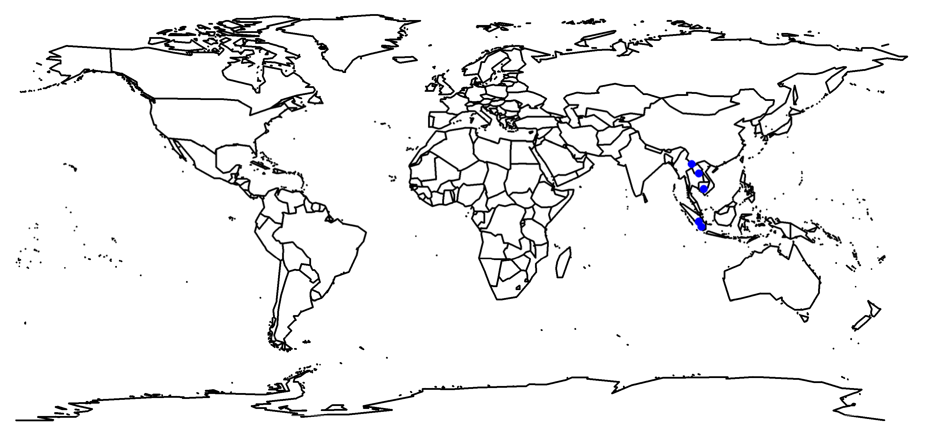
2.1. Study Sites
2.2. Model Initialization
2.3. Rubber PFT Development
2.4. Phenology
2.5. Phenology Scheme for Rubber
2.6. Allocation Scheme for Latex Harvest Yield
2.7. Tapping Period
2.8. Model Calibration
2.9. Rubber PFT Simulations and Evaluations
2.10. Comparing CLM-Rubber Model with Other Models
3. Results
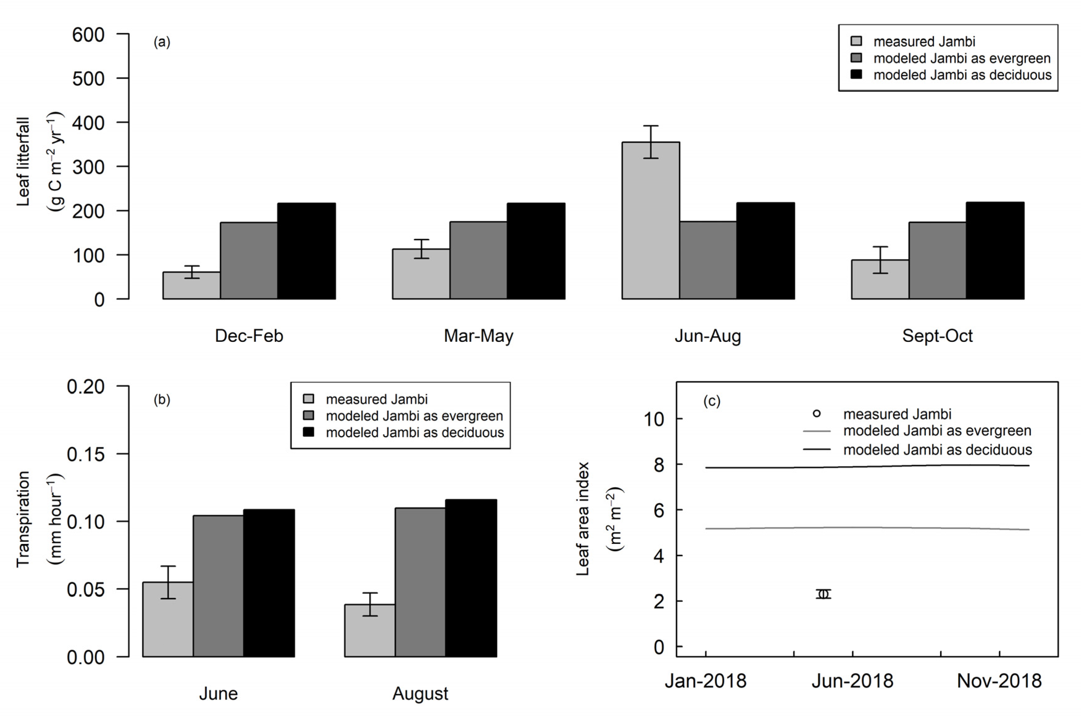
3.1. Rubber Modeled Using Alternate Tropical Forest Assumptions
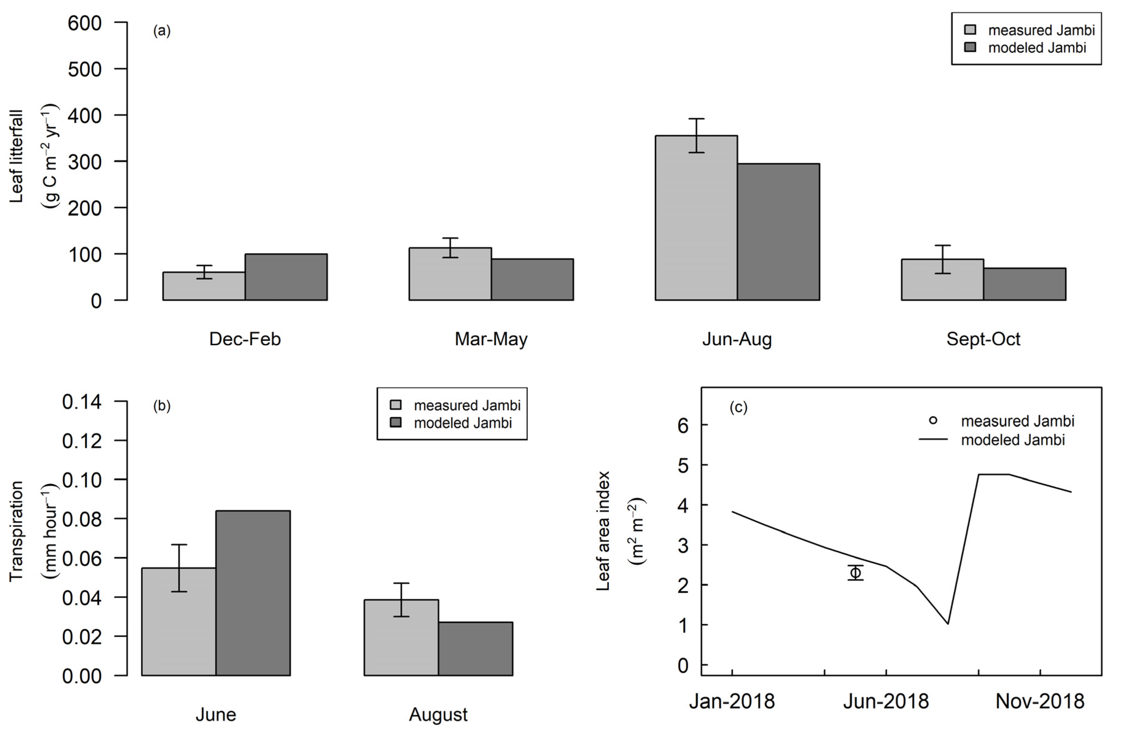
3.2. Phenology of Rubber in Jambi
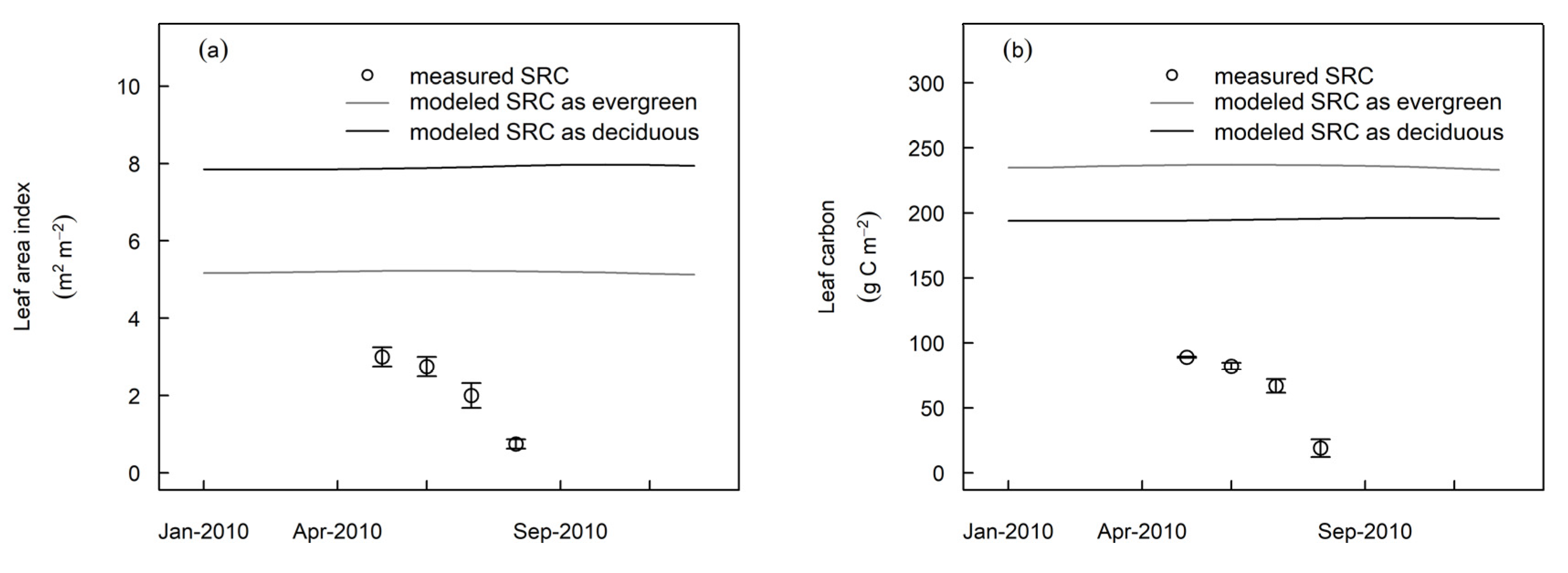
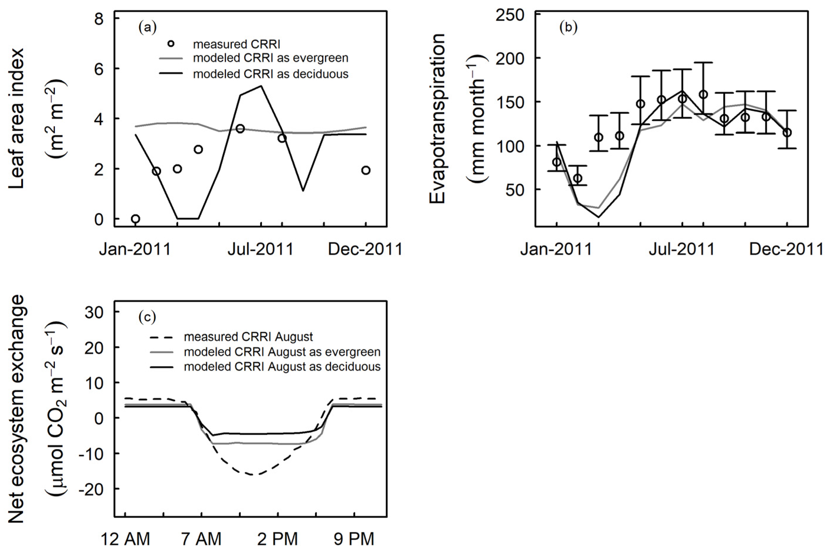
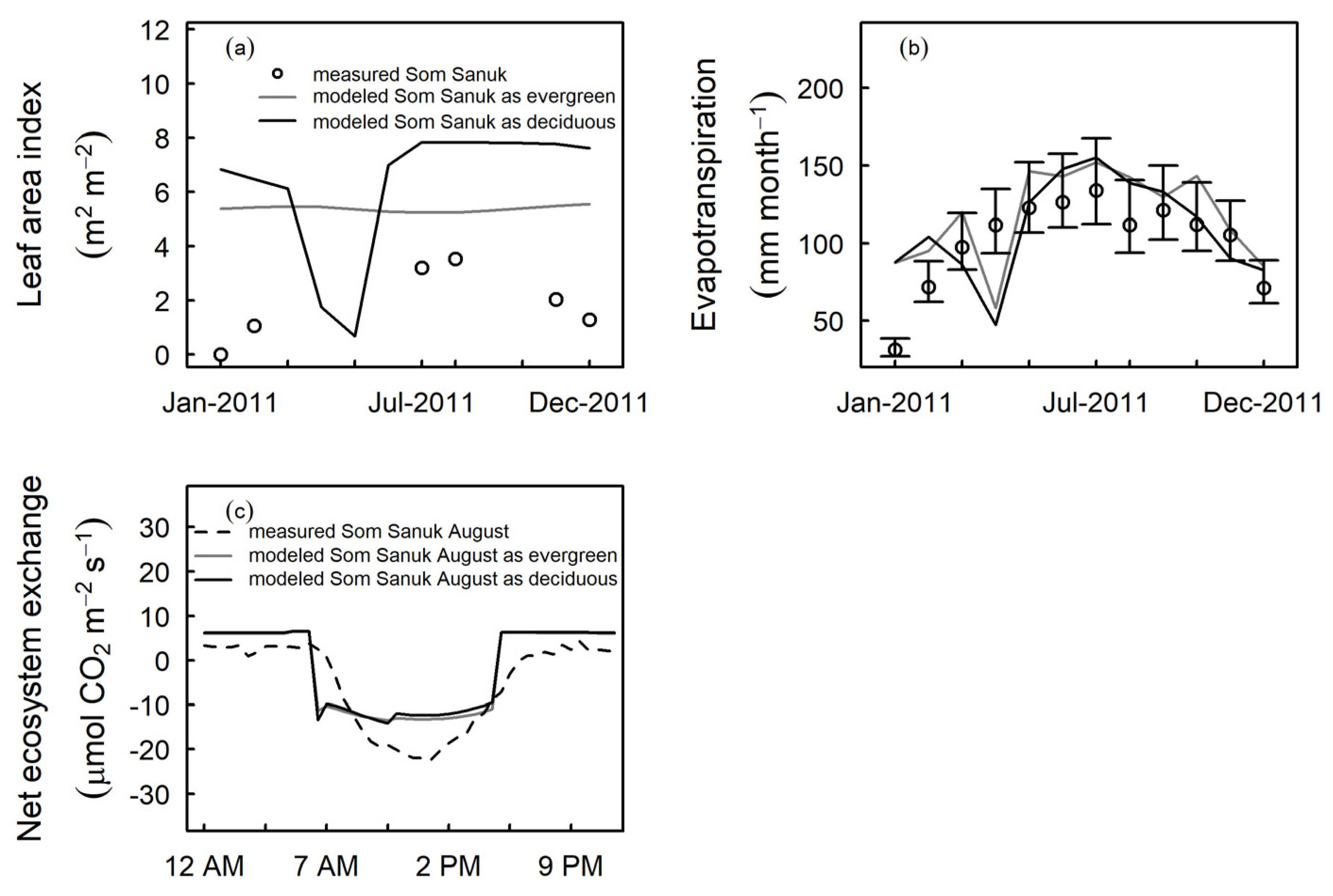
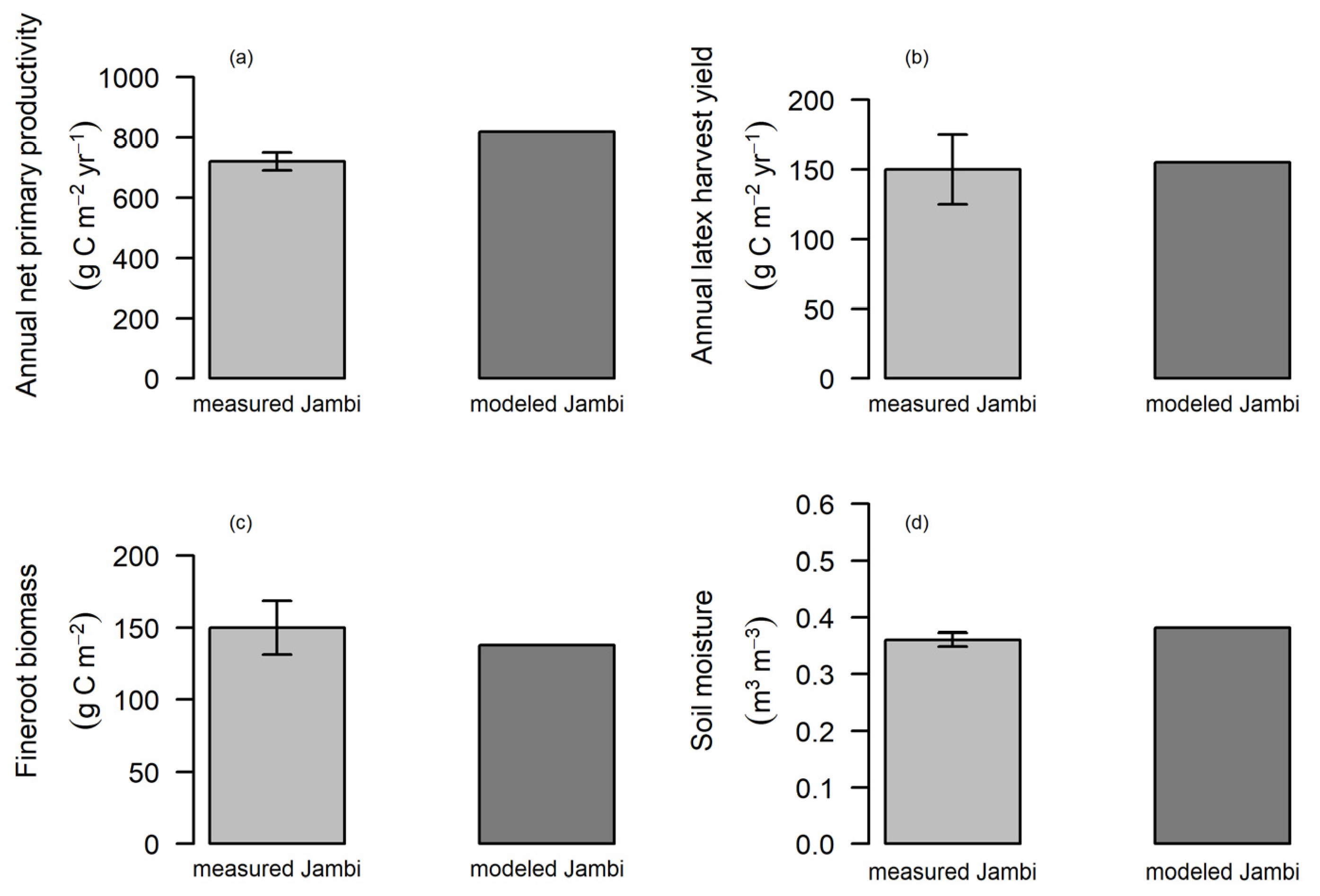
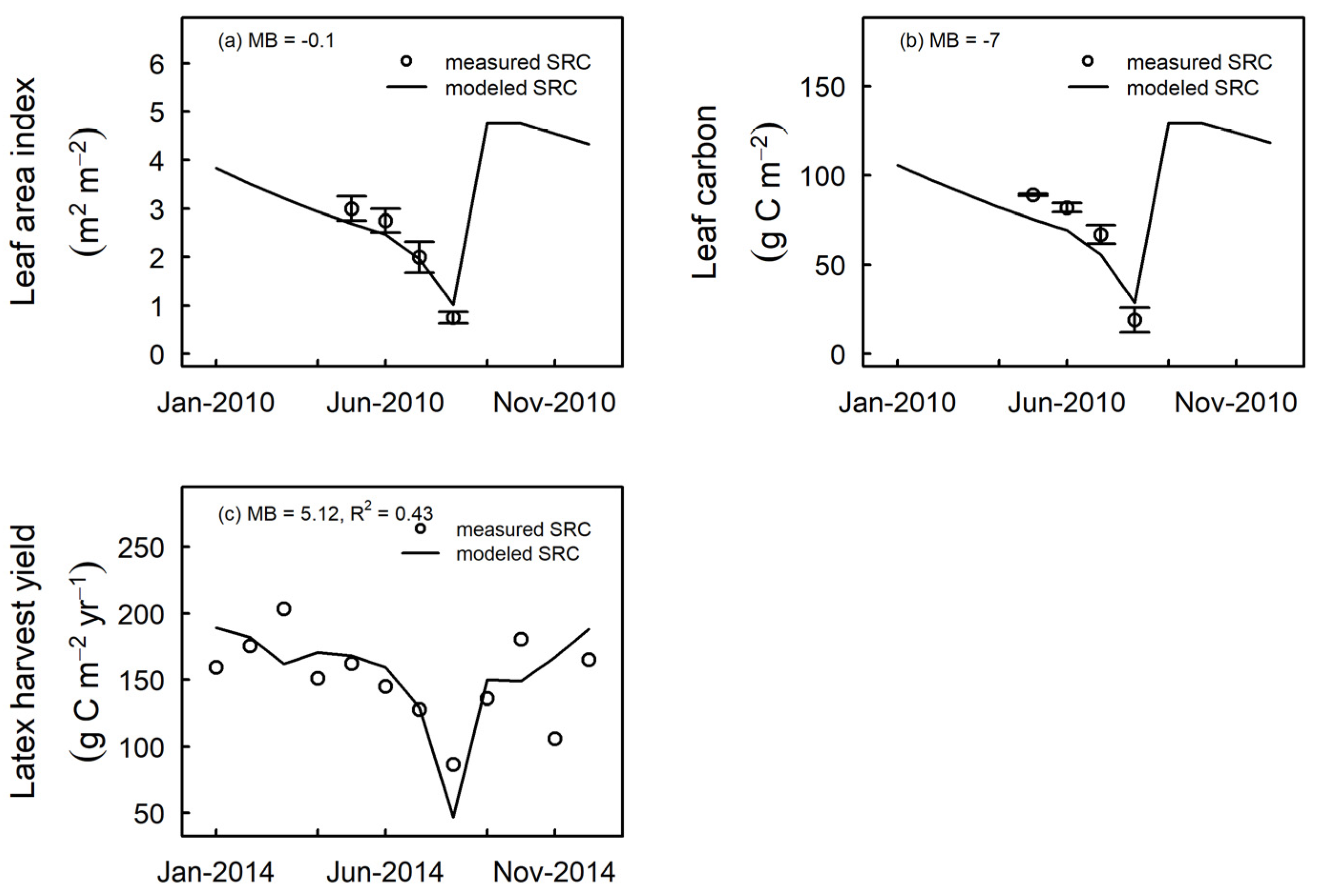
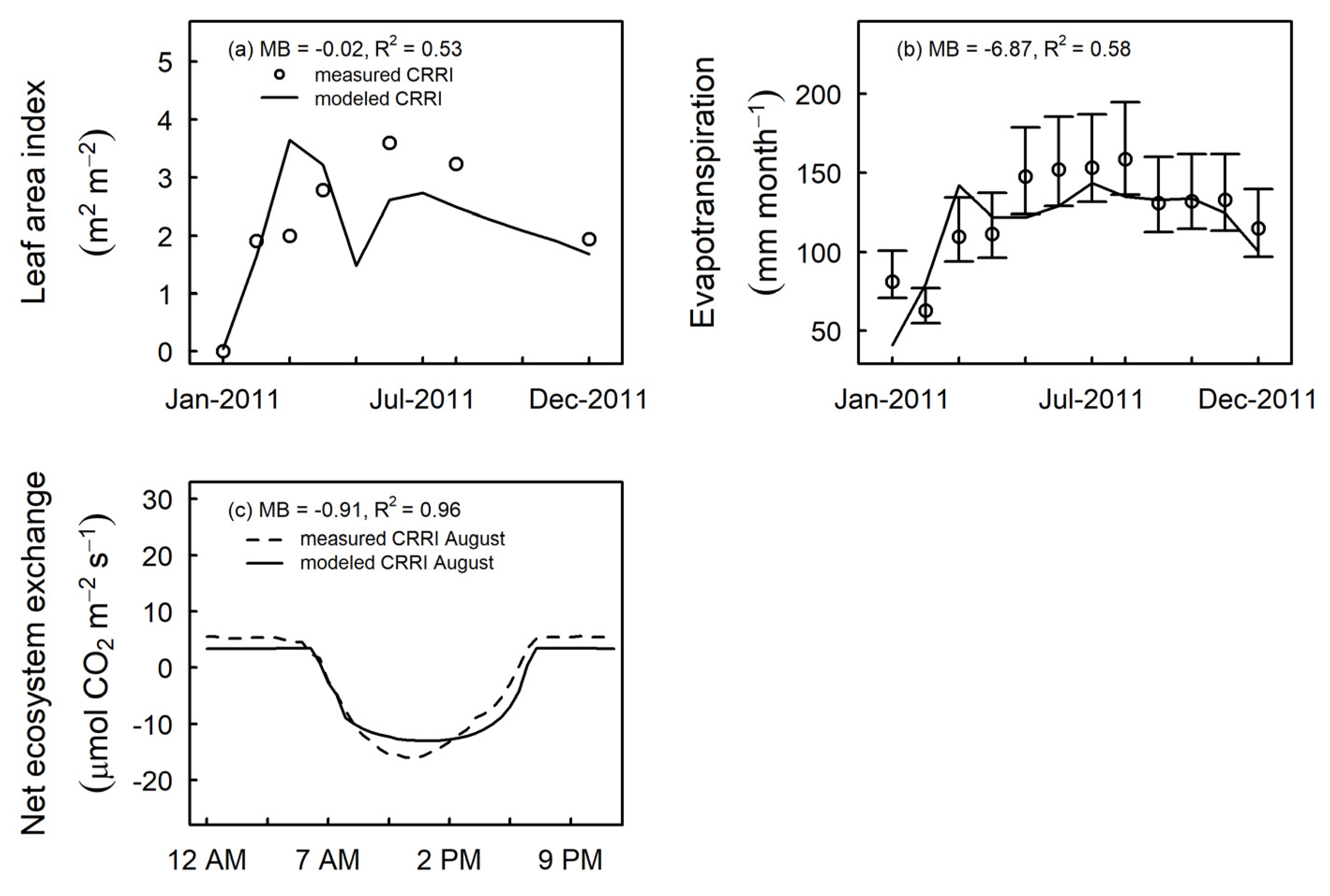
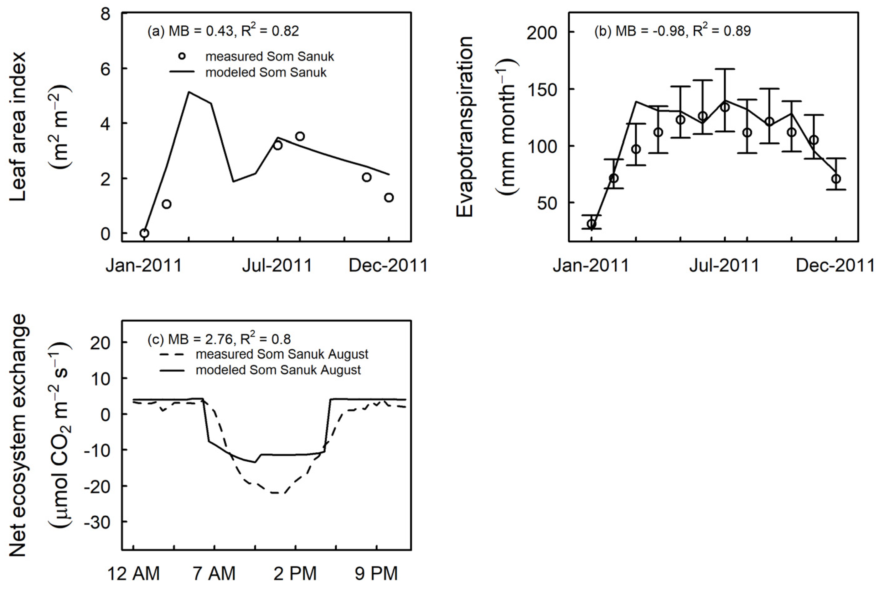
3.3. Model Evaluation at Independent Sites
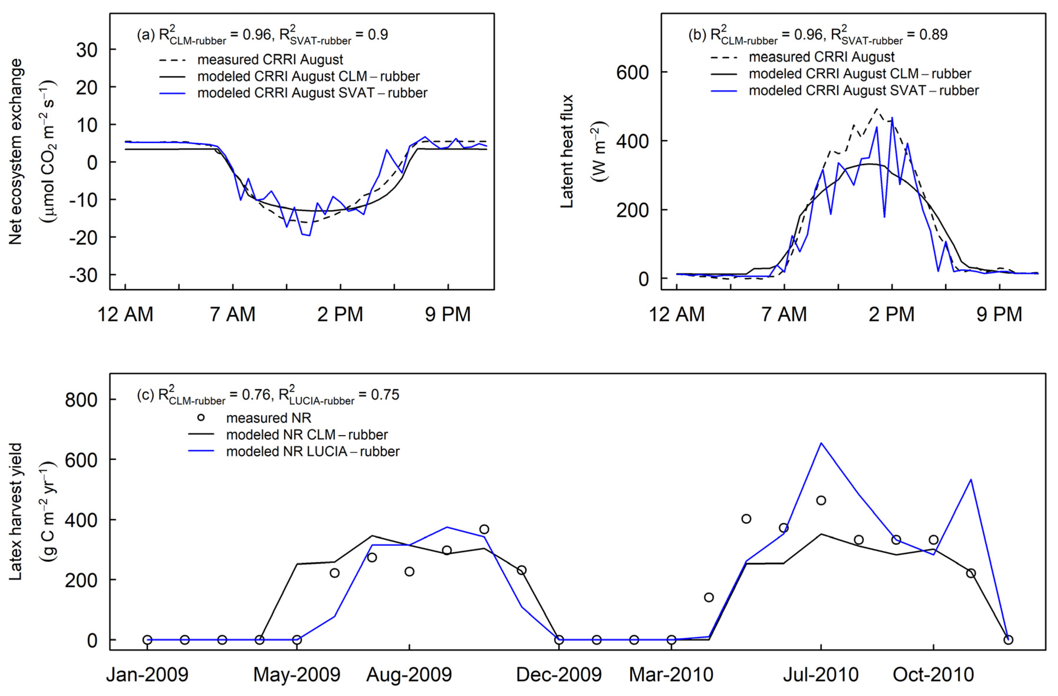
3.4. Comparing CLM-Rubber Model with Other Models
4. Discussion
4.1. Tropical Evergreen and Deciduous Simulations
4.2. Daylength, Carbon, and Water Fluxes
4.3. Intermodel Comparisons
5. Conclusions
Author Contributions
Funding
Institutional Review Board Statement
Informed Consent Statement
Data Availability Statement
Acknowledgments
Conflicts of Interest
Appendix A

Appendix B. Leaf Onset/Offset Parameterization
Appendix C. Background Leaf Litterfall
Appendix D. Allocation
References
- De Blécourt, M.; Brumme, R.; Xu, J.; Corre, M.D.; Veldkamp, E. Soil Carbon Stocks Decrease following Conversion of Secondary Forests to Rubber (Hevea brasiliensis) Plantations. PLoS ONE 2013, 8, e69357. [Google Scholar] [CrossRef] [PubMed]
- Röll, A.; Niu, F.; Meijide, A.; Ahongshangbam, J.; Ehbrecht, M.; Guillaume, T.; Gunawan, D.; Hardanto, A.; Hendrayanto; Hertel, D.; et al. Transpiration on the rebound in lowland Sumatra. Agric. For. Meteorol. 2019, 274, 160–171. [Google Scholar] [CrossRef]
- Ziegler, A.D.; Fox, J.M.; Xu, J. The Rubber Juggernaut. Science 2009, 324, 1024–1025. [Google Scholar] [CrossRef] [PubMed]
- Hurni, K.; Schneider, A.; Heinimann, A.; Nong, D.H.; Fox, J. Mapping the Expansion of Boom Crops in Mainland Southeast Asia Using Dense Time Stacks of Landsat Data. Remote Sens. 2017, 9, 320. [Google Scholar] [CrossRef]
- Senf, C.; Pflugmacher, D.; Van Der Linden, S.; Hostert, P. Mapping Rubber Plantations and Natural Forests in Xishuangbanna (Southwest China) Using Multi-Spectral Phenological Metrics from MODIS Time Series. Remote Sens. 2013, 5, 2795–2812. [Google Scholar] [CrossRef]
- Drescher, J.; Rembold, K.; Allen, K.; Beckschäfer, P.; Buchori, D.; Clough, Y.; Faust, H.; Fauzi, A.M.; Gunawan, D.; Hertel, D.; et al. Ecological and socio-economic functions across tropical land use systems after rainforest conversion. Philos. Trans. R. Soc. B Biol. Sci. 2016, 371, 20150275. [Google Scholar] [CrossRef]
- Lin, Y.; Zhang, Y.; Zhao, W.; Dong, Y.; Fei, X.; Song, Q.; Sha, L.; Wang, S.; Grace, J. Pattern and driving factor of intense defoliation of rubber plantations in SW China. Ecol. Indic. 2018, 94, 104–116. [Google Scholar] [CrossRef]
- Kositsup, B.; Kasemsap, P.; Thanisawanyangkura, S.; Chairungsee, N.; Satakhun, D.; Teerawatanasuk, K.; Ameglio, T.; Thaler, P. Effect of leaf age and position on light-saturated CO2 assimilation rate, photosynthetic capacity, and stomatal conductance in rubber trees. Photosynthetica 2010, 48, 67–78. [Google Scholar] [CrossRef]
- Kositsup, B.; Montpied, P.; Kasemsap, P.; Thaler, P.; Améglio, T.; Dreyer, E. Photosynthetic capacity and temperature responses of photosynthesis of rubber trees (Hevea brasiliensis Müll. Arg.) acclimate to changes in ambient temperatures. Trees 2008, 23, 357–365. [Google Scholar] [CrossRef]
- Giambelluca, T.W.; Mudd, R.G.; Liu, W.; Ziegler, A.D.; Kobayashi, N.; Kumagai, T.; Miyazawa, Y.; Lim, T.K.; Huang, M.; Fox, J.; et al. Evapotranspiration of rubber (Hevea brasiliensis) cultivated at two plantation sites in Southeast Asia. Water Resour. Res. 2016, 52, 660–679. [Google Scholar] [CrossRef]
- Kumagai, T.; Mudd, R.G.; Giambelluca, T.; Kobayashi, N.; Miyazawa, Y.; Lim, T.K.; Liu, W.; Huang, M.; Fox, J.; Ziegler, A.D.; et al. How do rubber (Hevea brasiliensis) plantations behave under seasonal water stress in northeastern Thailand and central Cambodia? Agric. For. Meteorol. 2015, 213, 10–22. [Google Scholar] [CrossRef]
- Allen, K.; Corre, M.D.; Tjoa, A.; Veldkamp, E. Soil Nitrogen-Cycling Responses to Conversion of Lowland Forests to Oil Palm and Rubber Plantations in Sumatra, Indonesia. PLoS ONE 2015, 10, e0133325. [Google Scholar] [CrossRef] [PubMed]
- van Straaten, O.; Corre, M.D.; Wolf, K.; Tchienkoua, M.; Cuellar, E.; Matthews, R.B.; Veldkamp, E. Conversion of lowland tropical forests to tree cash crop plantations loses up to one-half of stored soil organic carbon. Proc. Natl. Acad. Sci. USA 2015, 112, 9956–9960. [Google Scholar] [CrossRef] [PubMed]
- Cahyo, A.N.; Babel, M.S.; Datta, A.; Prasad, K.C.; Clemente, R. Evaluation of Land and Water Management Options to Enhance Productivity of Rubber Plantation Using Wanulcas Model. AGRIVITA J. Agric. Sci. 2016, 38, 93–102. [Google Scholar] [CrossRef][Green Version]
- Kumagai, T.; Mudd, R.G.; Miyazawa, Y.; Liu, W.; Giambelluca, T.W.; Kobayashi, N.; Lim, T.K.; Jomura, M.; Matsumoto, K.; Huang, M.; et al. Simulation of canopy CO2/H2O fluxes for a rubber (Hevea brasiliensis) plantation in central Cambodia: The effect of the regular spacing of planted trees. Ecol. Model. 2013, 265, 124–135. [Google Scholar] [CrossRef]
- Yang, X.; Blagodatsky, S.; Marohn, C.; Liu, H.; Golbon, R.; Xu, J.; Cadisch, G. Climbing the mountain fast but smart: Modelling rubber tree growth and latex yield under climate change. For. Ecol. Manag. 2019, 439, 55–69. [Google Scholar] [CrossRef]
- Liu, S.-J.; Zhou, G.-S.; Fang, S.-B.; Zhang, J.-H. Effects of future climate change on climatic suitability of rubber plantation in China. Ying Yong Sheng Tai Xue Bao 2015, 26, 2083–2090. [Google Scholar]
- Hazir, M.H.M.; Kadir, R.A.; Karim, Y.A. Projections on future impact and vulnerability of climate change towards rubber areas in Peninsular Malaysia. IOP Conf. Ser. Earth Environ. Sci. 2018, 169, 012053. [Google Scholar] [CrossRef]
- Ray, D.; Behera, M.; Jacob, J. Predicting the distribution of rubber trees (Hevea brasiliensis) through ecological niche modelling with climate, soil, topography and socioeconomic factors. Ecol. Res. 2016, 31, 75–91. [Google Scholar] [CrossRef]
- Lang, R.; Goldberg, S.; Blagodatsky, S.; Piepho, H.; Harrison, R.D.; Xu, J.; Cadisch, G. Converting forests into rubber plantations weakened the soil CH 4 sink in tropical uplands. Land Degrad. Dev. 2019, 30, 2311–2322. [Google Scholar] [CrossRef]
- Boisier, J.P.; De Nobletducoudre, N.; Pitman, A.; Cruz, F.T.; Delire, C.; Hurk, B.J.J.M.V.D.; van der Molen, M.; Müller, C.; Voldoire, A. Attributing the impacts of land-cover changes in temperate regions on surface temperature and heat fluxes to specific causes: Results from the first LUCID set of simulations. J. Geophys. Res. Space Phys. 2012, 117, 1–16. [Google Scholar] [CrossRef]
- Houghton, R.A.; House, J.I.; Pongratz, J.; Van Der Werf, G.R.; DeFries, R.S.; Hansen, M.C.; Le Quéré, C.; Ramankutty, N. Carbon emissions from land use and land-cover change. Biogeosciences 2012, 9, 5125–5142. [Google Scholar] [CrossRef]
- Pitman, A.J.; De Noblet-Ducoudré, N.; Cruz, F.T.; Davin, E.; Bonan, G.B.; Brovkin, V.; Claussen, M.; Delire, C.; Ganzeveld, L.; Gayler, V.; et al. Uncertainties in climate responses to past land cover change: First results from the LUCID intercomparison study. Geophys. Res. Lett. 2009, 36, 1–6. [Google Scholar] [CrossRef]
- Bonan, G.B.; Levis, S.; Kergoat, L.; Oleson, K.W. Landscapes as patches of plant functional types: An integrating concept for climate and ecosystem models. Glob. Biogeochem. Cycles 2002, 16, 5-1–5-23. [Google Scholar] [CrossRef]
- Fan, Y.; Meijide, A.; Lawrence, D.M.; Roupsard, O.; Carlson, K.M.; Chen, H.; Röll, A.; Niu, F.; Knohl, A. Reconciling Canopy Interception Parameterization and Rainfall Forcing Frequency in the Community Land Model for Simulating Evapotranspiration of Rainforests and Oil Palm Plantations in Indonesia. J. Adv. Model. Earth Syst. 2019, 11, 732–751. [Google Scholar] [CrossRef]
- Post, H.; Hendricks Franssen, H.-J.; Han, X.; Baatz, R.; Montzka, C.; Schmidt, M.; Vereecken, H. Evaluation and uncertainty analysis of regional-scale CLM4.5 net carbon flux estimates. Biogeosciences 2018, 15, 187–208. [Google Scholar] [CrossRef]
- Cheng, Y.; Huang, M.; Chen, M.; Guan, K.; Bernacchi, C.; Peng, B.; Tan, Z. Parameterizing Perennial Bioenergy Crops in Version 5 of the Community Land Model Based on Site-Level Observations in the Central Midwestern United States. J. Adv. Model. Earth Syst. 2020, 12, e2019MS001719. [Google Scholar] [CrossRef]
- Fisher, R.A.; Wieder, W.R.; Sanderson, B.M.; Koven, C.D.; Oleson, K.W.; Xu, C.; Fisher, J.B.; Shi, M.; Walker, A.P.; Lawrence, D.M. Parametric Controls on Vegetation Responses to Biogeochemical Forcing in the CLM5. J. Adv. Model. Earth Syst. 2019, 11, 2879–2895. [Google Scholar] [CrossRef]
- Lawrence, P.J.; Feddema, J.J.; Bonan, G.B.; Meehl, G.A.; O’Neill, B.C.; Oleson, K.W.; Levis, S.; Lawrence, D.; Kluzek, E.; Lindsay, K.; et al. Simulating the Biogeochemical and Biogeophysical Impacts of Transient Land Cover Change and Wood Harvest in the Community Climate System Model (CCSM4) from 1850 to 2100. J. Clim. 2012, 25, 3071–3095. [Google Scholar] [CrossRef]
- Dahlin, K.M.; Fisher, R.A.; Lawrence, P.J. Environmental drivers of drought deciduous phenology in the Community Land Model. Biogeosciences 2015, 12, 5061–5074. [Google Scholar] [CrossRef]
- Lawrence, D.M.; Fisher, R.A.; Koven, C.D.; Oleson, K.W.; Swenson, S.C.; Bonan, G.; Collier, N.; Ghimire, B.; van Kampenhout, L.; Kennedy, D.; et al. The Community Land Model Version 5: Description of New Features, Benchmarking, and Impact of Forcing Uncertainty. J. Adv. Model. Earth Syst. 2019, 11, 4245–4287. [Google Scholar] [CrossRef]
- Chen, M.; Griffis, T.J.; Baker, J.M.; Wood, J.D.; Xiao, K. Simulating crop phenology in the Community Land Model and its impact on energy and carbon fluxes. J. Geophys. Res. Biogeosci. 2015, 120, 310–325. [Google Scholar] [CrossRef]
- Wycherley, P.R. The Genus Hevea—Botanical Aspects. In Natural Rubber; Sethuraj, M.R., Mathew, N.M., Eds.; Developments in Crop Science; Elsevier: Amsterdam, The Netherlands, 1992; Volume 23, pp. 50–66. [Google Scholar] [CrossRef]
- Kotowska, M.M.; Leuschner, C.; Triadiati, T.; Hertel, D. Conversion of tropical lowland forest reduces nutrient return through litterfall, and alters nutrient use efficiency and seasonality of net primary production. Oecologia 2016, 180, 601–618. [Google Scholar] [CrossRef] [PubMed]
- Guardiola-Claramonte, M.; Troch, P.A.; Ziegler, A.D.; Giambelluca, T.W.; Vogler, J.B.; Nullet, M.A. Local hydrologic effects of introducing non-native vegetation in a tropical catchment. Ecohydrology 2008, 1, 13–22. [Google Scholar] [CrossRef]
- Yeang, H.-Y. Synchronous flowering of the rubber tree (Hevea brasiliensis) induced by high solar radiation intensity. New Phytol. 2007, 175, 283–289. [Google Scholar] [CrossRef]
- Zhai, D.-L.; Yu, H.; Chen, S.-C.; Ranjitkar, S.; Xu, J. Responses of rubber leaf phenology to climatic variations in Southwest China. Int. J. Biometeorol. 2019, 63, 607–616. [Google Scholar] [CrossRef]
- Song, Q.-H.; Tan, Z.-H.; Zhang, Y.-P.; Sha, L.-Q.; Deng, X.-B.; Deng, Y.; Zhou, W.-J.; Zhao, J.; Zhang, X.; Zhao, W.; et al. Do the rubber plantations in tropical China act as large carbon sinks? iForest-Biogeosci. For. 2013, 7, 42–47. [Google Scholar] [CrossRef]
- Bonan, G.B.; Lawrence, P.J.; Oleson, K.W.; Levis, S.; Jung, M.; Reichstein, M.; Lawrence, D.M.; Swenson, S.C. Improving canopy processes in the Community Land Model version 4 (CLM4) using global flux fields empirically inferred from FLUXNET data. J. Geophys. Res. Biogeosci. 2011, 116, 1–22. [Google Scholar] [CrossRef]
- Margono, B.A.; Turubanova, S.; Zhuravleva, I.; Potapov, P.; Tyukavina, A.; Baccini, A.; Goetz, S.; Hansen, M.C. Mapping and monitoring deforestation and forest degradation in Sumatra (Indonesia) using Landsat time series data sets from 1990 to 2010. Environ. Res. Lett. 2012, 7, 034010. [Google Scholar] [CrossRef]
- Ali, A.A.; Nugroho, B.; Moyano, F.E.; Brambach, F.; Jenkins, M.W.; Pangle, R.; Stiegler, C.; Blei, E.; Cahyo, A.N.; Olchev, A.; et al. Using a bottom-up approach to scale leaf photosynthetic traits of oil palm, rubber, and two coexisting tropical woody species. Forests 2021, 12, 359. [Google Scholar] [CrossRef]
- Kotowska, M.M.; Leuschner, C.; Triadiati, T.; Meriem, S.; Hertel, D. Quantifying above- and belowground biomass carbon loss with forest conversion in tropical lowlands of Sumatra (Indonesia). Glob. Chang. Biol. 2015, 21, 3620–3634. [Google Scholar] [CrossRef] [PubMed]
- Walker, A.P.; Hanson, P.J.; De Kauwe, M.G.; Medlyn, B.E.; Zaehle, S.; Asao, S.; Dietze, M.; Hickler, T.; Huntingford, C.; Iversen, C.M.; et al. Comprehensive ecosystem model-data synthesis using multiple data sets at two temperate forest free-air CO2 enrichment experiments: Model performance at ambient CO2 concentration. J. Geophys. Res. Biogeosci. 2014, 119, 937–964. [Google Scholar] [CrossRef]
- Fan, Y.; Roupsard, O.; Bernoux, M.; Le Maire, G.; Panferov, O.; Kotowska, M.M.; Knohl, A. A sub-canopy structure for simulating oil palm in the Community Land Model (CLM-Palm): Phenology, allocation and yield. Geosci. Model Dev. 2015, 8, 3785–3800. [Google Scholar] [CrossRef]
- Koven, C.D.; Riley, W.J.; Subin, Z.M.; Tang, J.Y.; Torn, M.S.; Collins, W.D.; Bonan, G.B.; Lawrence, D.M.; Swenson, S.C. The effect of vertically resolved soil biogeochemistry and alternate soil C and N models on C dynamics of CLM4. Biogeosciences 2013, 10, 7109–7131. [Google Scholar] [CrossRef]
- Viovy, N. CRUNCEP Version 7—Atmospheric Forcing Data for the Community Land Model; National Center for Atmospheric Research, Computational and Information Systems Laboratory: Boulder, CO, USA, 2018. [Google Scholar] [CrossRef]
- Meijide, A.; Badu, C.S.; Moyano, F.; Tiralla, N.; Gunawan, D.; Knohl, A. Impact of forest conversion to oil palm and rubber plantations on microclimate and the role of the 2015 ENSO event. Agric. For. Meteorol. 2018, 252, 208–219. [Google Scholar] [CrossRef]
- Li, Y.; Lan, G.; Xia, Y. Rubber Trees Demonstrate a Clear Retranslocation Under Seasonal Drought and Cold Stresses. Front. Plant Sci. 2016, 7, 1907. [Google Scholar] [CrossRef]
- Waite, P.-A. Variability of Wood and Leaffunctional Traits in Response to Structural and Environmental Changes in Natural and Transformed Systems in Indonesia. Ph.D. Thesis, University of Goettingen, Goettingen, Germany, June 2020. [Google Scholar]
- Priyadarshan, P.M. Biology of Hevea Rubber; CAB International: Wallingford, UK, 2011. [Google Scholar]
- Carr, M.K.V. The water relations of rubber (Hevea Brasiliensis): A review. Exp. Agric. 2012, 48, 176–193. [Google Scholar] [CrossRef]
- Perron, T.; Mareschal, L.; Laclau, J.-P.; Deffontaines, L.; Deleporte, P.; Masson, A.; Cauchy, T.; Gay, F. Dynamics of biomass and nutrient accumulation in rubber (Hevea brasiliensis) plantations established on two soil types: Implications for nutrient management over the immature phase. Ind. Crop. Prod. 2020, 159, 113084. [Google Scholar] [CrossRef]
- Chairungsee, N.; Gay, F.; Thaler, P.; Kasemsap, P.; Thanisawanyangura, S.; Chantuma, A.; Jourdan, C. Impact of tapping and soil water status on fine root dynamics in a rubber tree plantation in Thailand. Front. Plant Sci. 2013, 4, 538. [Google Scholar] [CrossRef]
- Zhou, R.; Zhang, Y.; Song, Q.; Lin, Y.; Sha, L.; Jin, Y.; Liu, Y.; Fei, X.; Gao, J.; He, Y.; et al. Relationship between gross primary production and canopy colour indices from digital camera images in a rubber (Hevea brasiliensis) plantation, Southwest China. For. Ecol. Manag. 2019, 437, 222–231. [Google Scholar] [CrossRef]
- Cahyo, A.N.; Ardika, R.; Wijaya, T. Water consumption and rubber production on various planting space arrangement system and their relationship with soil water content. Indones. J. Nat. Rubber Res. 2011, 29, 110–117. [Google Scholar]
- Oktavia, F.; Lasminingsih, M. Effect of rubber plant leaves development to production variation in IRR series clones. Indones. J. Nat. Rubber Res. 2010, 28, 32–40. [Google Scholar]
- Chantuma, P.; Lacointe, A.; Kasemsap, P.; Thanisawanyangkura, S.; Gohet, E.; Clement, A.; Guilliot, A.; Ameglio, T.; Thaler, P. Carbohydrate storage in wood and bark of rubber trees submitted to different level of C demand induced by latex tapping. Tree Physiol. 2009, 29, 1021–1031. [Google Scholar] [CrossRef] [PubMed]
- Silpi, U.; Lacointe, A.; Kasempsap, P.; Thanysawanyangkura, S.; Chantuma, P.; Gohet, E.; Musigamart, N.; Clement, A.; Ameglio, T.; Thaler, P. Carbohydrate reserves as a competing sink: Evidence from tapping rubber trees. Tree Physiol. 2007, 27, 881–889. [Google Scholar] [CrossRef]
- Barman, R.; Jain, A.K.; Liang, M. Climate-driven uncertainties in modeling terrestrial gross primary production: A site level to global-scale analysis. Glob. Chang. Biol. 2014, 20, 1394–1411. [Google Scholar] [CrossRef]
- Ali, A.A.; Xu, C.; Rogers, A.; Fisher, R.A.; Wullschleger, S.D.; Massoud, E.C.; Vrugt, J.A.; Muss, J.D.; McDowell, N.G.; Fisher, J.B.; et al. A global scale mechanistic model of photosynthetic capacity (LUNA V1.0). Geosci. Model Dev. 2016, 9, 587–606. [Google Scholar] [CrossRef]
- Whitley, R.J.; Macinnis-Ng, C.M.O.; Hutley, L.; Beringer, J.; Zeppel, M.; Williams, M.; Taylor, D.; Eamus, D. Is productivity of mesic savannas light limited or water limited? Results of a simulation study. Glob. Chang. Biol. 2011, 17, 3130–3149. [Google Scholar] [CrossRef]
- Schaefer, K.; Schwalm, C.; Williams, C.A.; Arain, M.A.; Barr, A.; Chen, J.M.; Davis, K.J.; Dimitrov, D.; Hilton, T.; Hollinger, D.Y.; et al. A model-data comparison of gross primary productivity: Results from the North American Carbon Program site synthesis. J. Geophys. Res. Space Phys. 2012, 117, 1–15. [Google Scholar] [CrossRef]
- Ankomah, G.O. Assessment of Leaf Area Index and Canopy Openness Across Four Land-Use Systems in Jambi Province, Sumatra, Indonesia. Master’s Thesis, University of Goettingen, Goettingen, Germany, March 2019. [Google Scholar]
- Niu, F.; Röll, A.; Meijide, A.; Hendrayanto; Hölscher, D. Rubber tree transpiration in the lowlands of Sumatra. Ecohydrology 2017, 10, e1882. [Google Scholar] [CrossRef]
- Hassler, E.; Corre, M.D.; Tjoa, A.; Damris, M.; Utami, S.R.; Veldkamp, E. Soil fertility controls soil–atmosphere carbon dioxide and methane fluxes in a tropical landscape converted from lowland forest to rubber and oil palm plantations. Biogeosciences 2015, 12, 5831–5852. [Google Scholar] [CrossRef]
- Igarashi, Y.; Katul, G.; Kumagai, T.; Yoshifuji, N.; Sato, T.; Tanaka, N.; Tanaka, K.; Fujinami, H.; Suzuki, M.; Tantasirin, C. Separating physical and biological controls on long-term evapotranspiration fluctuations in a tropical deciduous forest subjected to monsoonal rainfall. J. Geophys. Res. Biogeosci. 2015, 120, 1262–1278. [Google Scholar] [CrossRef]
- Dawoe, E.K.; Isaac, M.E.; Quashie-Sam, J. Litterfall and litter nutrient dynamics under cocoa ecosystems in lowland humid Ghana. Plant Soil 2010, 330, 55–64. [Google Scholar] [CrossRef]
- Hirata, R.; Saigusa, N.; Yamamoto, S.; Ohtani, Y.; Ide, R.; Asanuma, J.; Gamo, M.; Hirano, T.; Kondo, H.; Kosugi, Y.; et al. Spatial distribution of carbon balance in forest ecosystems across East Asia. Agric. For. Meteorol. 2008, 148, 761–775. [Google Scholar] [CrossRef]
- Ali, A.A.; Fan, Y.; Corre, M.D.; Kotowska, M.M.; Hassler, E.; Cahyo, A.N.; Moyano, F.E.; Stiegler, C.; Röll, A.; Meijide, A.; et al. Data and Codes for a Rubber Plant Functional Type in the Community Land Model (CLM5). 2021. Available online: https://zenodo.org/record/4729044#.Ye5Mr6ERV9A (accessed on 30 April 2021).
- Oleson, K.; Lawrence, D.; Bonan, G.; Drewniak, B.; Huang, M.; Koven, C.; Levis, S.; Li, F.; Riley, W.; Subin, Z.; et al. Technical Description of Version 4.5 of the Community Land Model (CLM); National Center for Atmospheric Research: Boulder, CO, USA, 2013. [Google Scholar] [CrossRef]


| Parameter | Definition | Unit | Default/ Baseline Value | Rubber Parameter Value | Parameter Type | Modeled Outcomes the Parameter Value Impacts |
|---|---|---|---|---|---|---|
| SWPc | Critical soil water potential (SWP) | MPa | −0.8 | −2 or −0.8 | calibrated value |
|
| rho | Factor that multiplies the rate coefficient for background litterfall | unitless | 1 | 1.5 | calibrated value |
|
| ftap | Proportion of latex tapping for wood allocation partitioning | unitless | − | 0.46 | calibrated value |
|
| SLA | Specific leaf area | m2 g−1C | 0.0308 | 0.026 | measured value from literature |
|
| Leaf longevity | Life of leaf | years | 0.483 | 1 | calibrated value |
|
| Stem: leaf | Ratio of stem C to leaf C | unitless | 2.3 | 1 | calibrated value |
|
| leafcn | Leaf C: N | g C g−1 N | 23.45 | 14.7 | measured value from literature |
|
| leafcn_max | Maximum leaf CN ratio | g C g−1 N | 35 | 25.3 | measured value from literature |
|
| leafcn_min | Minimum leaf CN ratio | g C g−1 N | 15 | 10.5 | measured value from literature |
|
| dsladlai | Change is specific leaf area per unit change in leaf are index | m2 g−1 C | 0.0027 | 0.0012 | calibrated value |
|
| medlynslope | Medlyn slope of conductance–photosynthesis relationship | µmol H2O µmol−1 CO2 | 4.45 | 3.56 | calibrated value |
|
Publisher’s Note: MDPI stays neutral with regard to jurisdictional claims in published maps and institutional affiliations. |
© 2022 by the authors. Licensee MDPI, Basel, Switzerland. This article is an open access article distributed under the terms and conditions of the Creative Commons Attribution (CC BY) license (https://creativecommons.org/licenses/by/4.0/).
Share and Cite
Ali, A.A.; Fan, Y.; Corre, M.D.; Kotowska, M.M.; Preuss-Hassler, E.; Cahyo, A.N.; Moyano, F.E.; Stiegler, C.; Röll, A.; Meijide, A.; et al. Implementing a New Rubber Plant Functional Type in the Community Land Model (CLM5) Improves Accuracy of Carbon and Water Flux Estimation. Land 2022, 11, 183. https://doi.org/10.3390/land11020183
Ali AA, Fan Y, Corre MD, Kotowska MM, Preuss-Hassler E, Cahyo AN, Moyano FE, Stiegler C, Röll A, Meijide A, et al. Implementing a New Rubber Plant Functional Type in the Community Land Model (CLM5) Improves Accuracy of Carbon and Water Flux Estimation. Land. 2022; 11(2):183. https://doi.org/10.3390/land11020183
Chicago/Turabian StyleAli, Ashehad A., Yuanchao Fan, Marife D. Corre, Martyna M. Kotowska, Evelyn Preuss-Hassler, Andi Nur Cahyo, Fernando E. Moyano, Christian Stiegler, Alexander Röll, Ana Meijide, and et al. 2022. "Implementing a New Rubber Plant Functional Type in the Community Land Model (CLM5) Improves Accuracy of Carbon and Water Flux Estimation" Land 11, no. 2: 183. https://doi.org/10.3390/land11020183
APA StyleAli, A. A., Fan, Y., Corre, M. D., Kotowska, M. M., Preuss-Hassler, E., Cahyo, A. N., Moyano, F. E., Stiegler, C., Röll, A., Meijide, A., Olchev, A., Ringeler, A., Leuschner, C., Ariani, R., June, T., Tarigan, S., Kreft, H., Hölscher, D., Xu, C., ... Knohl, A. (2022). Implementing a New Rubber Plant Functional Type in the Community Land Model (CLM5) Improves Accuracy of Carbon and Water Flux Estimation. Land, 11(2), 183. https://doi.org/10.3390/land11020183