Peer Effects in Housing Size in Rural China

Abstract

In recent decades, rural China has witnessed a housing construction boom. In order to control the rapid growth of rural housing, both central and local governments have established quantitative restrictions on the floor numbers and total housing area; however, these have been relatively ineffective. Current research to explain this rapid growth in rural housing tends to consider independent household behavior, while social interactions among villagers are neglected. Therefore, the aim of this article is to examine the existence of peer effects in the housing size of villagers and whether they differ among different regions to better understand the influence of social interactions on individual housing behaviors, especially in the context of rural China. A spatial autoregressive model with autoregressive disturbances (SARAR) was used to analyze data from the 2014 China Family Panel Studies (CFPS). The results confirm that villagers’ peer effects do exist, indicating that rural households build housing not only to satisfy their dwelling needs but also to keep up with the other villagers’ housing size. Moreover, there are regional disparities in terms of peer effects in rural housing size. Among the three regional parts, the undeveloped region in the western parts showed the largest peer effects. Therefore, local governments, especially from the underdeveloped region, should pay attention to the villagers’ inner motivations behind housing behavior.

1. Introduction

Rural China has changed rapidly and profoundly since the economic reforms in 1978 [1]. In terms of spatial restructuring, rural housing construction has boomed due to the miniaturization of the family structure, the reconfiguration of the economic activities of rural households, and the increasing wealth earned by out-migration [2,3]. From 1978 to 2019, the average housing size per capita has grown from 8.1 m² to 48.9 m², a more than four-fold increase. Enthusiasm for rural housing construction has also led to problems such as rural housing land sprawl, farmland erosion, and rural hollowing [4,5]. Therefore, since the 1990s, both central and local governments have established rigid quantitative restrictions for rural housing land and rural housing size, while also punishing overdue construction [6,7]. For example, in 2019, it was required by Heyuan Municipality that the total floor numbers in rural housing were restricted to three and a half. In the case of Guizhou Province, residential construction area was limited to 320 m² per household in 2021. However, though the regulations for rural housing construction have been established for quite a while, most of them cannot keep pace with rural housing development, and illegal and disordered constructions remain an issue [2,8]. If this inefficiency in spatial resource usage continues, it will be difficult to realize the target of sustainable development raised in the “Rural Development Promotion Law” [9].

Increasingly, scholars and policy makers have attempted to understand the enthusiasm surrounding rural housing construction. Top–down policy failures in controlling rural housing size indicate that policy makers should also consider the villagers’ internal motivations. Consequently, it is of great importance that the villagers’ motivations behind their housing construction behavior are revealed. Past research on rural housing construction has shown that residential improvement needs, membership for future return, and potential rental profits are all motivations for rural housing construction and are enabled by increasing income [3,10,11]. However, researchers have found that acquiring relative status and showing off success can also increase the demands of conspicuous goods such as housing [12]. In this way, housing construction behavior should not be considered an independent household decision, as it is also shaped by social interactions with villagers nearby. Therefore, it is reasonable to ask whether rural housing may actually be a follow-up of the construction behavior of village peers. Moreover, uneven developments in the eastern, central, and western parts of China have been reflected in rural housing [13,14]. Therefore, it is also reasonable to ask whether the peer effect shows regional disparities.

In housing research, housing is customarily regarded as a tool to satisfy residential and investment needs, which are studied under the framework of individual demand and supply [15]. However, it is recently increasingly accepted that housing also plays a role as a status good [16], the demand of which is also influenced by social interactions with other people. The notion that social interactions among group members in shaping individual behavior has been applied to many research fields, but research in housing is still limited [17,18]. Current research on social interactions in shaping housing behavior mainly focus on Western housing markets such as in Spain or the USA [19], and its existence in a Chinese context requires examination. Additionally, whether social actions in housing behavior differ among regions with different development levels needs further research.

This brings us to the aim of this paper. First, notwithstanding the notion of housing as a conspicuous good becoming increasingly accepted worldwide, whether social interactions in groups influence an individual’s housing behavior is still an interesting topic in housing research, especially in the context of rural China. Considering the tight networks in rural China, it is reasonable to infer that individual housing behavior would be influenced by other villagers. Besides, the housing market has not been established in rural China, making villagers less likely to build housing for investment purposes and more likely for residential and status needs. Therefore, this paper examines whether social interactions among villagers, namely peer effects, influence their housing behavior in a rural Chinese context. Second, considering the uneven developments in regions in the past decades, different parts of China may have quite different cultures and development levels. Therefore, this paper also examines the regional disparity in terms of peer effects. By exploring whether social interactions among villagers influence housing size, this research contributes to the body of knowledge regarding rural housing in China. First, it goes beyond earlier studies on rural housing in China by considering housing not as an independent household decision, but as being shaped by social interactions among villagers nearby. Second, it examines the existence of social interactions in housing behavior in a different context—rural China. Third, it extends the body of literature by examining whether social actions in housing differ among regions with different development levels.

The rest of the paper is organized as follows. Section 2 introduces the history of rural housing growth and government-related policies. Section 3 provides a brief literature review on peer effects, especially peer effects in housing behavior. Section 4 describes the theoretical framework, variable description, and model design. Section 5 provides the model results. Section 6 concludes the main findings, makes a comparison with similar studies, and discusses the theoretical implications. Section 7 proposes policy implications, discusses study limitations, and shows future research directions.

2. Rural Housing in China

Housing is the most expensive item in one’s lifetime and is a crucial determinant of the subjective well-being for most people. People need housing in terms of three housing values, namely residential value, investment value, and status value. The housing consumption outcomes such as housing size and housing tenure are considered as a balance between housing market supply and household housing demand [20]. Many theories were raised to explain the household housing outcomes worldwide from both the macro level and micro level. Theories at the micro level include the neoclassic consumption theory, life cycle theory, housing filtering theory, gradient consumption theory, and so on [21]. In general, household needs, household financial capacity, and external market environment would influence the household housing outcomes. Factors such as socio-economic condition (age, education, marital status, family size, household income), social network, housing market condition, and housing policies are usually considered when analyzing household housing outcomes.

In the Western world, the housing market is the main mechanism of both urban and rural housing resource allocation. Most housing research is located in an urban context, but rural housing research is gaining in popularity. In the post-World War II period, rural areas were initially treated as economically dependent on urban areas [22]. Since the 1990s, the local action and endogenous development of rural areas were given more attention [23]. Rural areas’ uniqueness of less density, natural environment, and policy context make rural housing quite different from urban housing and worthy of further research. Despite various types of rural areas worldwide, there are some common research topics in rural housing studies including gentrification, landscape preservation, and so on. For example, some rural counties in the United States have gone through the exurbanization process and attracted retirees and second-home owners [24]. In England, rural “locals” often become displaced by counter-urbanization processes, leading to acute affordability issues in rural England [25].

In the context of China, the socio-economic conditions in rural areas are quite different from Western countries. In particular, the housing market has not been established in rural China. Unlike the deregulated housing trade and rent in urban areas and urban villages, the housing trade is still under strict regulation in rural areas. Rural villagers commonly live in self-constructed houses [3]. In this way, rural housing in China is segregated from the urban housing market, and provides residential and status function without an investment function. In rural housing research, both residential land area and housing size can be used to measure the housing outcomes, but housing size was less used for data availability. Therefore, instead of focusing on research of rural housing size, the following paragraph gives a general context on the evolution of rural housing in China.

Rural housing has an extensive history in China [2]. According to growth rate and government policy, the development of rural housing can be classified into three stages. The first stage is the slow growth stage from 1949 to 1978. After the founding of the People’s Republic of China in 1949, the Rural Collective Land Property was gradually formed, namely collective ownership and individual using rights, and rural housing was considered individual property that was protected by the constitution [26,27]. During that period, the growth in rural housing was slow due to low income from collective farming jobs and the Chinese traditional norm of generations sharing houses (so-called “si shi tong tang”). If villagers lived in a capacious house, it would have been considered as a form of capitalism.

The second stage, from 1978 to 1995, was the period of “both rural housing and the rural population increase”. Since the opening-up policy in 1978, China has experienced a rapid transition from a central planning economy to a market-based economy, and the rural ‘‘Household Responsibility System” greatly stimulated rural economic growth. Many farmers became wealthier, and they began to prefer multi-functional, more comfortable, or spacious houses, making the rural household model of “si shi tong tang” decline in popularity [2]. Therefore, rural housing demands grew rapidly with the reconfiguration of rural households’ economic activities and social aspirations, triggering waves of rural housing construction. From 1978 to 1995, the rural resident population increased from 790 million to 859 million. The average construction area (referred as “average area” in the following) per person also increased from 8.1 m² to 21.0 m², indicating that rural housing areas were increasing faster than rural populations [28]. However, the enthusiasm for rural housing led to problems such as cultivated land shrinkage, rural hollowing, and land resource waste [2,12,29]. Under these circumstances, China’s central government established the national specialized bureau of land management (“guojia tudi guanliju”), set restrictions for the application of rural housing land, and created punitive policies against illegal behavior in order to conserve arable land from the excessive occupation of housing construction [6]. For example, the procedure for applying for rural residential land was required by the State Council in 1982, and residential land was limited to one lot per household [3,30]. However, these measures were not so effective because of the difficulties related to supervising rural land.

The third stage was from 1996 to the present, the transitional period of “rural population decrease but rural housing land increase”. With the new round of market-oriented economic reforms and the flexible hukou system, the rural resident population decreased from 704 in 1996 to 671 million in 2008 [31,32]. Under the condition of large-scale out- migration, a substantial amount of income earned in urban areas was reinvested in rural housing construction. As a result, rural housing land continued to expand despite the shrinking rural population. From 2000 to 2008, rural housing land expanded from 16.53 million ha to 16.66 million ha at an annual growth rate of 0.1%, while per capita rural housing land (PRHL) increased from 204.5 m² to 231.0 m² at an annual growth rate of 1.6% [4,33,34]. As such, the governments became more aware of farmland protection, so more exact policies and techniques were introduced to supervise rural land. For example, it was made explicit by law that rural households were prohibited from applying for more than one housing lot [35,36], while hollowed villages and idle land were investigated and cleaned up gradually by the Ministry of Land and Resources thanks to the “Opinions about strengthening of rural homestead management” [6]. As a result, rural housing land expansion slowed down a little, whereas the enthusiasm for rural housing did not decrease. From 1996 to 2007, average housing area per capita increased from 21.7 m² to 31.6 m² at an annual rate of 3.47%. From 2008 to 2019, average housing area per capita increased from 32.4 m² to 48.9 m² at an annual rate of 3.81%, which was even faster compared to 1996 to 2007 [37]. Meanwhile, multiple floors replaced farmland occupation, gradually gaining popularity among villagers as a way to build large houses. In 2011, the central government initiated a policy to restrict floor numbers and the height of each floor [7], but only recently, local provinces such as Guizhou, Sichuan, and Fujian have begun restricting rural housing to three floors.

The expansion of rural settlements has not been sufficiently curbed by the decreasing rural population, and government regulations are ineffective in controlling housing construction in rural areas, which has aroused great research interest [2,8]. Research on rural housing development is embedded in a wide context and various factors. The first explanation, which is widely accepted, is the increase in socio-economic developmental level caused by rural-to-urban migration. The rapid increase in migration affected the rural economy in the late 1990s [10,11,38,39]. Migrants went to eastern seaboard coastal regions for economic opportunities and sent their remittance back home, making housing improvements economically feasible. Second, some researchers hold the opinion that migrants build housing to ensure their membership due to their future plans for returning. In cities, migrant workers are not granted permanent household registration, are excluded from many social welfare entitlements, and are still subjected to socioeconomic, institutional, and cultural discrimination, making returning home in the future more appealing [40]. Third, villagers close to major urban areas and towns with high land values tend to build large houses for potential rental profits [3,41]. Fourth, villagers build large houses as conspicuous assets and symbols of success [8,12]. As with other institutions in rural areas that lack well-functioning markets, migration can play a complex role in asset accumulation. Following this conformity to building more housing assets [42], villagers can achieve identity and social status within a village and become competitive in terms of marriage options and credit market [43,44,45].

3. Peer Effects and Housing

There is increasing recognition that social interactions, in other words, interdependencies between individuals, play an important role in describing and explaining individual decisions and behaviors. Peer effects have been indicated as important determinants, described as a reference group’s influence on individual behavior. Reference groups such as neighborhoods, family, classmates, etc. may include a subgroup of individuals with single ties with others, or all members of the entire group might share the same social norms. The type (directional or reciprocated) and degree (strong or weak) of peer effect may differ among individuals and is determined by ability, effort, or other unobservable factors [46]. Peer effects exist in a wide range of individual behaviors such as education, labor markets, fertility, obesity, etc. [19,47].

Many potential methods have been applied to identify and estimate social interactions in recent years, and one of the most often used models was proposed by Manski [48]. In his model, three effects (endogenous, contextual, and correlated effects) were raised to explain why individuals belonging to the same group tend to behave similarly. Endogenous effects refer to an individual’s tendency to vary with the prevalence of certain behaviors within a given group. Exogenous (contextual) effects, however, represent the propensity of an individual to behave in some way that varies with the exogenous characteristics of a group. Correlated effects imply that individuals tend to behave similarly because they have similar individual characteristics in a given group or face similar institutional environments. While others’ outcome in the same group affects individual decisions, the inverse is also true. Many studies on peer effects use either school-fixed effects or instrumental variable regression techniques to model endogenous interactions [49]. Recent advances in spatial econometrics make it possible to estimate social interaction effects, which have been shown to improve identification [50,51].

The mechanism through which the peer effect is widespread includes many forms, and conformity is one that can influence preferences [48]. Conformism is the idea that when people evaluate their behavior, if it lacks an objective standard, they will tend to choose groups that share similarities. Conformity makes group members more likely to try their best to blend in with their peer group’s surroundings and choose to keep up with the majority of members [52]. In general, conformity preferences in terms of peer effects are regarded as a social norm, and individuals within a peer group will attain potential benefits if they obey the norms; otherwise, they may suffer by deviating from it. In theory, the incentive origin for conformism stems from peer pressures and partnerships, religion, social status and social distance, and crime [53,54,55,56,57,58,59,60].

However, despite the long history of research about the effect of social interactions on individual behavior, the literature regarding social interactions in housing research is still extremely limited, and mainly focuses on Western housing markets such as Spain, the USA, etc. [61]. A taste for conformity that captures the idea of “keeping up with the Joneses” has been found in fields such as housing price, housing size, housing quality, and housing satisfaction, indicating that individuals view the reference group’s decisions on housing consumption and investment to keep up by making similar decisions [18,62,63,64,65,66,67]. Representative research such as that by Ioannides and Zabel estimated neighborhood effects in housing renovation decisions [68]. Beamonte analyzed neighborhood effects in housing price with spatiotemporal autoregressive models [63]. Patacchini and Venanzoni investigated the social interactions in housing quality using detailed data of friendship networks [18]. The effect of social interactions highlights the tendency of individuals to view housing as a symbol of status and prestige [69]. In this sense, housing is not just a good that satisfies dwelling needs, but also a “positional good” that satisfies the desire for relative status. Motivated by positional concerns, all members of a society are working more for wealth and conspicuous consumption to gain status. However, this tendency may result in a “positional treadmill” [69]. As everyone is heading toward the same direction, the relative position of individuals in a society is unchangeable, so no one is happier.

Rural China is not only a suitable case in which to examine the effect of social interactions on housing behavior, but it can also offer new perspectives regarding the regional disparity in terms of peer effects. Compared to Western countries, rural China is more of an acquaintance society, where social interactions among rural households are relatively long-term and stable. As a result, rural households in China are more likely to be influenced by interactive relationships, follow social norms, and desire a favorable social image in their own community [70]. In recent years, village norms depict “the best housing” as a beautiful, modern villa that demonstrates wealth and “face” and helps to attract marriage and business partners [49]. In this context, it is reasonable to predict that rural households may be deeply influenced by their reference group in their housing behavior. Considering the uneven development of China, this influence may have regional disparity. However, because of the state–collective divide in land ownership, the housing behavior in rural areas is quite different from urban areas, and has not been as well studied as in the urban housing market [27,71,72]. Therefore, this paper aims to contribute more evidence for the peer effect in housing and its regional disparity in China.

Therefore, this paper empirically reveals peer effects on China’s rural housing, which contributes to current research in two ways. First, rural housing in China is unique in its strong cultural conformity norms, making it a perfect place to explore the peer effect theory that is rarely touched in housing research. Second, using a spatial econometric method to estimate housing size, this paper not only explores social interactions among villagers quantitively, but also alleviates the estimation bias generated by traditional ordinary least-squares (OLS) models.

4. Data and Methodology

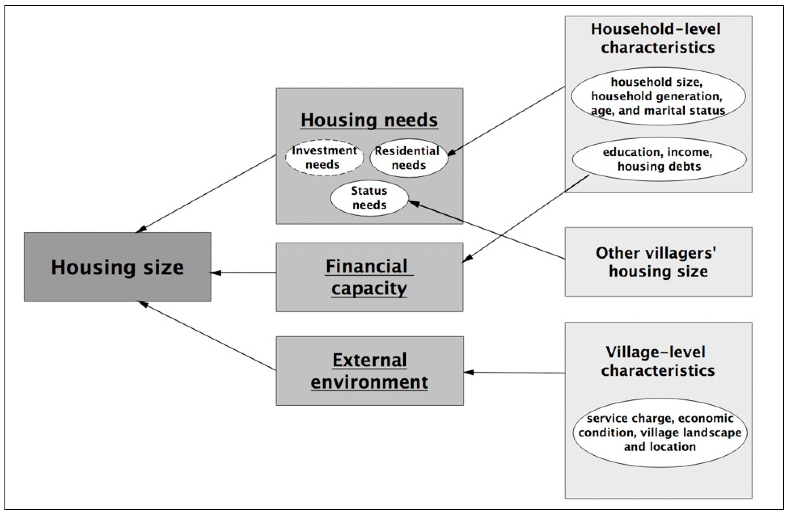
4.1. Theoretical Framework

Housing has three types of function, namely residential function, investment function, and status function. The investment function should not be considered because the selected villages are not located in towns or cites where housing have rental profits. Therefore, villagers located in typical rural areas build housing only for residential needs and status needs. We developed a conceptual model to explain the villagers’ housing outcomes, namely, housing size in this paper (Figure 1). According to current research, housing size can be influenced by household housing needs, household financial capacity, and external environment. The residential housing needs could be influenced by household life cycle such as household size, household generation, household head’s age, and marital status. The status housing needs could be influenced by other villagers’ housing outcomes. The household financial capacity could be influenced by education, income, and debts. The external environment could include the service charge, economic condition, village landscape, and location. In this way, factors influencing rural housing size can be classified into household-level characteristics, village-level characteristics, and other villager’s housing size.

4.2. Data

This study uses the data from the2014 China Family Panel Studies (CFPS). CFPS is a national longitudinal annual survey conducted by the Institute of Social Science Survey at Peking University since 2010, designed to investigate family well-being and its dynamics in contemporary China. By using a rural–urban integrated sampling frame, the 2014 data via computer-assisted personal interviews, interviewed 13,946 households, and 57,739 family members living at home, from 621 communities across 25 mainland provinces/cities/autonomous regions. This survey is representative of the 25 provinces/cities/autonomous by using an implicit stratification, multi-stage, multi-level, and probability proportional size-sampling method [73].

The family in CFPS refers to an economically independent dwelling unit with at least one family member of Chinese nationality. Family members in the survey refers to (1) all immediate relatives who are economically interdependent (“tong zao chi fan”); and (2) all non-immediate relatives who have been living in the household continuously for three months or longer. Note that a key criterion CFPS uses to identify family relationships is economic rather than current residence; people who have left home for school or work but have a close economic relationship with other members of the household are treated as family members. Family size in our research refers to the number of family members, and the concept of family members is in accordance with the CFPS definition.

In the 2014 survey, the CFPS included a family questionnaire and a family member questionnaire that examined family constitution (each family members’ age, education, and other demographic information), family financial capacity (households’ deposits, housing debts, annually income), and housing condition (housing property, housing source, the area of housing) in detail. In this paper, we measure the housing size by using the construction area of the current residence owned by this household1. The reason we used the 2014 CFPS data instead of the 2018 CFPS data was that only the 2014 CFPS data contained the community-level questionnaire, asking about each community’s population structure, location and transportation, and economic condition.

We focused on the household excerpts from rural villages. According to the literature above-mentioned, other factors such as land consolidation and suburban investment may contribute to rural housing construction enthusiasm, so we needed to separate villages that were not in typical rural areas through sample selection. First, we excluded residential communities located in cities and towns, and rural villages that had gone through land expropriation by governments. Second, we excluded households who did not have ownership of their housing. Third, we excluded villages that had fewer than ten interviewees to ensure that we could gather enough interviewees within each village and investigate the conformity behavior within the village. Fourth, we excluded households that either could not respond or did not respond properly. This yielded a total number of 3057 valid households from 23 provinces and 166 villages2.

The basic characteristics of the participants are listed in

Table 1. Sample profile.

Variables	Variables Description	Observation	Mean/ Percentage	Standard Deviation
Household characteristics
Housing size	The housing area of current residence (m2)	3057	152.15	117.49
Household size	Number of family members who are economically related (person)	3057	4.21	1.94
Household generation	The number of family generations (dai)	3057	2.32	0.82
Household income per capita	Total income per capita last year (CNY 10,000)	3057	0.98	1.12
Housing debts	Housing debts at present or not	3057
	0 = No		77.43%
	1 = Yes		22.57%
Household head age	The age of household head	3057	50.60	12.61
Household head marital status	The marital status of household head
	0 = Unmarried, divorced or widowed		9.98%
	1 = Married		90.02%
Household head education	The education of household head	3057
	0 = No education		32.19%
	1 = Primary school		28.92%
	2 = Middle school		28.62%
	3 = High school and above		10.27%
Village characteristics
Service charge	Price for hiring housing-construction Skilled workers per day (CNY)	166	174.34	53.40
Landscape	Landscape type	166
	0 = Plateaus, mountains or other types		25.88%
	1 = Plains and hills		74.12%
Distance to town	Distance to the nearest town (km)	166	10.22	16.55
Distance to county	Distance to the nearest county (km)	166	51.74	36.56
Distance to provincial capital	Distance to the nearest provincial capital (km)	166	568.09	660.77
Village income per capita	The annual net income per capita of village (CNY 10,000)	166	0.48	0.44

. For the selected 3057 villagers, the average housing size was 152.15 m². The average household size was about four persons, and the average generation was 2.32. Therefore, the average housing size per capital was about 38 m², which was quite similar but slightly lower compared to the 2014 national statistical data of 41.45 m². The average age of household heads was around 50 years old. About 90% of household heads were married. The average household income per capital was about CNY 9800, and 22.57% of the households had current housing debts. Most of the household heads had received no education. The average cost of a skilled worker for housing construction for one day is about CNY 174. The majority of the villages are located on the plains and hills, and only 25.88% of the villages are located on plateaus, mountains, or other types. The average distance to town, county, and provincial capital are 10.22 km, 51.74 km, and 568.09 km, respectively, indicating that the selected villages are typical villages away from urban areas. The average village incomes per capita was around CNY 4800 last year.

Table 2. Average area per household of rural housing by province.

Region	Provinces	Number of Villages	Number of Observations	Average Housing Area per Household
East	Liaoning	13	271	105.63
	Hebei	13	229	150.08
	Shandong	7	134	149.46
	Tianjin	1	22	222.27
	Jiangsu	1	13	98.46
	Zhejiang	2	30	96.50
	Fujian	2	33	202.24
	Guangdong	15	249	143.60
	Total	54	981	137.12
Middle	Heilongjiang	3	58	77.50
	Jilin	3	52	82.31
	Shanxi	11	199	166.94
	Anhui	2	38	134.71
	Henan	25	503	189.26
	Hubei	1	11	236.73
	Hunan	3	48	187.73
	Jiangxi	4	80	218.16
	Total	52	989	173.28
West	Shaanxi	6	111	121.98
	Yunnan	6	125	145.98
	Guizhou	8	105	139.46
	Sichuan	8	128	155.55
	Chongqing	1	12	138.75
	Guangxi	4	71	123.79
	Gansu	27	535	154.19
	Total	60	1087	146.48
All	In total	166	3057	152.15

shows that there is regional divergence in rural housing size. The average housing sizes per household for eastern, middle, and western China were 137.12 m², 173.28 m², and 146.48 m². It turns out that the villagers in eastern provinces, who were wealthier than villagers in middle and western provinces, actually had the smallest residential space. Despite the fact that the selected sample was not strictly representative of China’s rural households, we can still examine the peer effects in different regions separately.

4.3. Models

In order to separate the peer effect from other effects, we referred to the terms raised by Manski, which explained three effects (endogenous, contextual, and correlated effects) through which individual behavior may show similarities within a group. In our research, we tried to investigate whether an endogenous effect exists in rural housing. In rural China, village membership is mostly determined by their family name and kinship. Therefore, the self-selection of villagers into villages was not considered.

Rural housing in the same village was not independent of each other, thus violating the assumption of the traditional OLS estimation. Therefore, the spatial econometrics method, which considers social interaction effects, was employed to avoid biased estimation. Among all the spatial models such as the spatial lag model (SAR), the spatial error model (SEM), the spatial Durbin model (SDM), the spatial lagged X model (SLX), the spatial Durbin error model (SDEM), etc., the more general model is the general nesting spatial model (GNS), which subsumes all the spatial dependence and heterogeneity effects. However, the GNS model is weakly identified, and it is difficult to simultaneously account for three sources of effects statistically. The main strategy to solve this problem is to constrain one of the spatial parameters to zero. Therefore, we used the spatial autoregressive model with autoregressive disturbances (SARAR) model in the following equation, which includes both the spatial lag term and the spatially correlated error.

The empirical equivalent of our SARAR model of peer effects is given by:

y = λWy + Xβ + μ

(1)

μ = ρMμ + ε

(2)

where Y is the housing size of the current residence of each household; W and M are n × n spatial weight matrix; and X is the set of control variables of household characteristics. Villagers from the same village were considered as the reference group, so let Wij = 1, Mij = 1 if the individuals came from the same village. Afterward, we normalized the spatial weights matrix. λWY is the Y lagged by the spatial matrix of W, which reflects the influence of other villagers’ housing size on the individual’s housing size. Here, the individual villager increased utility from keeping up with the other villagers’ housing behavior, namely, housing size in this research. λ is the parameter describing the taste for conformity or strength of the peer effect, which is usually between 0 and 1. If λ is statistically significant in the SARAR model, we can prove the existence of peer effect. Besides, the larger λ is, the larger the peer effects. The Xβ is controlled including some household characteristics to control the contextual effects and some village characteristics to control the correlated effects. μ reflects other unobservable variables in the disturbances that may also have spatial interactions and are used to control the correlated effects. In a word, after controlling these variables, λ is what we focused on the most. Through the estimation of λ, we can prove that villagers construct their housing not only to satisfy their own residential needs, but also to keep up with their fellow villagers.

The OLS regression was carried out to diagnose the existence of spatial effects. As

Table 3. Diagnostic tests for spatial dependence in the ordinary least-squares (OLS) regression.

Test	Statistic	p-Value
Spatial lag:
Lagrange multiplier	1413.437	0.000
Robust Lagrange multiplier	51.798	0.000
Spatial error:
Moran’s I	38.096	0.000
Lagrange multiplier	1361.850	0.000
Robust Lagrange multiplier	0.211	0.000

shows, both the spatial lag of the dependent variable and spatial errors should be considered. In this circumstance, the generalized spatial two-stage least square (GS2SLS) method was used to evaluate the model; this is more suitable than the maximum likelihood estimation (MLE) method when heteroscedasticity exists in a large sample.

5. Results

5.1. Conformity Preference

This paper includes a non-interactive OLS model (Model 1) as a “benchmark” for a comparison with the SARAR model (Model 2) in

Table 4. Estimation results of the rural housing size of the whole country.

	Model 1	Model 2	Model 3	Model 4	Model 5
Dependent Variable:	OLS	GS2SLS	GS2SLS	GS2SLS	GS2SLS
Housing Size (m2)	Coefficient	Coefficient	Direct Effect	Indirect Effect	Total Effect
Household Characteristics
Household size	6.803 ***	3.520 ***	9.228	−5.921	3.306
Household generation	4.501	2.786	7.304	−4.687	2.617
Household income per capita	7.884 ***	5.157 ***	13.521	−8.676	4.845
Have housing debts	15.446 **	10.679 **	27.998	−17.966	10.032
Household head age	0.118	0.126	0.330	−0.212	0.118
Household head marital status	17.218 ***	17.068 ***	44.750	−28.716	16.034
Household head edu
Primary school	13.789 **	9.147 **	23.982	−15.389	8.593
Middle school	10.439 **	6.058 *	15.882	−10.192	5.691
High school and above	20.168 ***	13.608 **	35.677	−22.894	12.783
Village Characteristics
Service charge	0.025	0.007	0.019	−0.012	0.007
Plains and hills	13.947 ***	1.020	2.675	−1.716	0.958
Distance to town	−0.549 ***	−0.083 ***	−0.218	0.140	−0.078
Distance to county	−0.471 ***	−0.069 ***	−0.180	0.116	−0.065
Distance to provincial capital	0.009 **	0.002	0.004	−0.003	0.001
Village income per capita	−6.928	−0.622	−1.631	1.046	−0.584
Intercept	84.687	−30.238
Spatial autocorrelation variable
λ		0.841 ***
ρ		−1.622 ***
Number of observations	3057	3057	3057	3057	3057

Note: ***, **, and * denote significance at 1%, 5%, and 10%, respectively.

. Both the OLS model and GS2SLS model were statistically significant, and the adjusted R-squares were 0.070 and 0.083, respectively. However, the estimates of the spatial autoregressive coefficient λ were our primary interest. In the SARAR model, λ is significantly positive (λ = 0.841), which means endogenous effects do exist, even when other effects are controlled. This result conclusively supports our assumption that villagers build houses not only for residential needs, but also to keep up with other villagers. Therefore, the villagers’ housing behaviors are not independent. In general, rural housing area is built for rural norms (i.e., “less housing, lower recognition from others” (“meiyou fangzi meiyou diwei”). Because λ is statistically significant, we can prove the existence of peer effects in housing size.

The results of cumulative direct, indirect, and total effects are respectively reported in Model 3, Model 4, and Model 5. We refer to Golgher and Voss’s (2016) research to calculate the direct effects and indirect effects [74]. By using the β, λ, and spatial weight matrix from Model 2, we can calculate the partial derivative matrix for variables. The existence of off-diagonal elements of the partial derivatives matrix mean the existence of spillover effects. Specifically, the summary measure of the individual direct effects is the mean of the diagonal terms of the partial derivative matrix. The summary measure of individual indirect effects (spillover effects) is a cumulative measure that sums the off-diagonal elements across rows (or columns) and divides by the number of rows (columns) to obtain an average spillover effect. The direct effect means that changes of an explanatory variable in an individual have direct effects on oneself. The indirect effects mean that changes in an explanatory variable in an individual have effects on others, which are also known as the spatial spillovers. The total effects are the sum of the direct and indirect effects. Specifically, from Model 3 to Model 5, the direct effects indicate that a change in an explanatory variable in a villager impacts that villager’s housing size, while indirect effects measure how a change in an explanatory variable influences other villagers’ housing size. Comparing the effects of explanatory variables on housing size, the coefficients of direct effects are larger than those of indirect effects, indicating that individual housing size is mainly influenced by direct effects.

The household characteristics were used to control, proving that “keeping up with the Joneses” behavior is not due to individual villagers’ similarities. All the household characteristics were quite significant in both the OLS model and the SARAR model, which implies that individual similarity contributes to similar housing outcomes. In detail, the coefficient of household size was 3.520, which confirms our common notion that more family members create more residential needs. Both the household head’s age and household generation were not significant. The household head’s marital status was highly significant, showing that compared to unmarried, divorced, or widowed villagers, married villagers more likely build larger housing. The household income per capita, the housing debts, and household head’s education were all significant variables, revealing the importance of economic capacity in enlarging housing size. With the miniaturization of Chinese households and the influence of marital status and family size on housing size, it is quite reasonable to require that residential land should be limited to one lot per household.

Village characteristics control correlative effects, proving that “keeping up with the Joneses” behavior is not due to similar background characteristics from the same village. Most of the village characteristics are significant in the OLS model. Landscape, which has been frequently neglected by previous research, turns out to have significant explanatory power. Under the same circumstances, if the landscape of a village is characterized by plains or hills, the housing size will be 14 m² larger than houses on plateaus, mountains, or other types of landscape. The service charge for construction was not significant. A village’s macro location also matters. In the OLS model, the distance to a town or county has a negative effect, while the distance to a provincial city has a positive effect. The increase in distance will raise the transportation cost, then reduce the housing size. Village income per capita is not significant, the information of which is included in other variables. In the SARAR model, most of the village variables change into insignificance after introducing the spatial interactions in the disturbances. Only the distance to town and distance to county have significant power, indicating that the town and the county are more influential in rural housing construction compared to the provincial capital. Considering the fact that rural housing size is influenced by the village’s macro location, it is quite reasonable to set local quantitative restrictions and requirements in different places.

The coefficient for spatial error ρ was statistically significant, proving that, despite the significant variables above, there are still some spatial effects that are not controlled by the above variables. Additionally, the changes in coefficient in Model 1 and Model 2 were quite small. The inclusion of spatial autocorrelation makes the model more reasonable, so the SARAR models provide better estimation.

5.2. Regional Disparity

The results of the endogenous effect among the three regions are presented separately in

Table 5. Estimation results of rural housing size by the spatial autoregressive model with autoregressive disturbances (SARAR) model across the three regions.

	East	Middle	West
Dependent Variable: Housing Size (m2)	Coefficient (Robust Standard Error)	Coefficient (Robust Standard Error)	Coefficient (Robust Standard Error)
Household Characteristics
Household size	0.986 (0.641)	2.794 (1.858)	1.325 ** (0.629)
Household generation	−0.923 (2.340)	7.783 * (4.571)	−2.322 *** (1.981)
Household income per capita	1.242 * (0.648)	1.828 * (1.047)	0.793 (0.764)
Have housing debts	2.174 (4.495)	19.175 *** (6.732)	3.013 (4.549)
Household head age	0.012 (0.099)	0.139 (0.208)	0.136 (0.092)
Household head marital status	0.904 (3.942)	24.301 *** (7.171)	11.495 ** (5.218)
Household head edu
Primary school	5.635 * (2.990)	10.953 (7.100)	3.311 (4.532)
Middle school	3.945 (2.713)	7.851 (6.204)	−0.398 (4.111)
High school and above	3.612 (4.441)	24.483 * (13.480)	1.920 (6.250)
Village Characteristics
Service charge	−0.007 (0.007)	−0.006 (0.018)	0.005 (0.012)
Plains and hills	0.159 (1.251)	2.148 (3.671)	−0.271 (1.320)
Distance to town	0.087 * (0.051)	−0.005 (0.035)	−0.039 (0.042)
Distance to county	−0.023 (0.032)	−0.066 (0.076)	−0.012 (0.001)
Distance to provincial capital	0.001 (0.001)	−0.001 (0.002)	0.001 (0.001)
Village income per capita	0.126 (0.694)	−1.137 (4.026)	0.677 (2.985)
Intercept	−4.996 (6.759)	−53.083 (18.549)	−17.858 (6.504)
Spatial autocorrelation variable
λ	0.958 *** (0.044)	0.863 *** (0.035)	0.976 *** (0.044)
ρ	−4.891 *** (1.453)	−1.844 *** (0.588)	−5.497 *** (1.874)
Number of observations	981	989	1087

Note: ***, **, and * denote significance at 1%, 5%, and 10%, respectively.

. The coefficients for spatial autocorrelation variable λ were significant in all three regions, and the values were 0.958, 0.863, and 0.976, respectively. The different values of λ in the three models provide evidence that peer effects differ among regions. This conclusion reinforces the importance of considering the endogenous effect of “keeping up with the Joneses” on a local level. The λ in western provinces was the largest, which means that villagers in western provinces, compared to the other two regions, have the largest motivation for building more housing to conform with their village peers. The λ in the eastern provinces and in the western provinces were quite similar, but still smaller than in the western provinces. The λ in the middle provinces were the smallest. In a word, the villagers in the western provinces were most concerned about their village peers and conforming with the housing construction behavior of others. This difference in terms of social interaction may result from economy disparities. Since the western region is the poorest among the three, traditional culture and conformity may be kept well and valued the most.

Most of the variables in Table 5 play the same role as the coefficients in Table 4, except for some special cases. In the western region, variables related to life cycle such as household size, household generation, and household head marital status were significant. While variables related to household economic capacity such as household income per capita, have housing debts, and household head education were not significant, the results highlight that household residential need, rather than financial capacity, is the constraining factor in the western region. In the middle region, household head marital status, household generation, have housing debts, and household head education were significant, showing that both household residential need and financial capacity were constraining factors in the middle region. In the eastern region, household income per capita and household head education were significant, showing the importance of household financial capacity. The distance to three types of economic center nearly all changed into insignificance among the three regions. One exception is that being close to town may decrease housing size, which may be due to the scarce land resources near town in the eastern region. Considering the above, the western provinces are where traditional values of conformity are more ingrained.

5.3. Robust Test

We conducted the robust test using the 2010 CFPS data3 in

Table 6. Estimation results of the 2010 CFPS data.

	2010 GS2SLS Model
Dependent Variable: Housing Size (m2)	Coefficient (Robust Standard Error)
Household Characteristics
Household size	2.995 *** (0.971)
Household generation	4.906 ** (2.361)
Household income per capita	0.506 * (0.291)
Have housing debts	13.712 *** (3.597)
Household head age	0.153 (0.113)
Household head marital status	5.676 (4.406)
Household head edu
Primary school	1.895 (3.337)
Middle school	13.441 *** (3.494)
High school and above	10.086 ** (4.669)
Village Characteristics
Service charge	0.060 (0.037)
Plains and hills	1.814 (1.565)
Distance to town	0.008 (0.062)
Distance to county	−0.056 (0.043)
Distance to provincial capital	0.001 (0.003)
Village income per capita	−0.001 (0.002)
Intercept	−23.015 (10.783)
Spatial autocorrelation variable
λ	0.805 *** (0.056)
ρ	−0.866 ** (0.444)
N	3057

Note: ***, **, and * denote significance at 1%, 5%, and 10%, respectively.

. The coefficient for spatial autocorrelation λ was also significant, indicating the existence of peer effects in both 2010 and 2014. Besides, the λ for the 2010 data was 0.805, smaller than 0.841 for the 2014 data, indicating that the spatial autocorrelation variable increased over time. We also ran the panel SAC model to include both the 2010 and 2014 data. The λ in the panel model was still significant, showing that the results were robust. The results of the panel SAC model were not shown in the paper.

6. Discussion

China has gradually evolved into an urban country, which presents challenges to the continuing rural population in terms of demographic structures, employment opportunities, community organization, lifestyles, standards of living, accessibility, and rural culture [1,75,76,77,78,79]. In terms of spatial transformation, new housing construction behavior in rural China has increased, arousing the interest of both researchers and the government. The enthusiasm for rural housing construction, originating in 1978, has led to problems such as cultivated land shrinkage, rural hollowing, and land resource waste. Therefore, both central and local governments have proposed rigid regulations regarding rural housing land and housing size, which were effective at slowing down the growth rate, but ineffective in totally controlling unorderly construction. As a result, many scholars have raised various reasons to explain this rural housing growth such as socio-economic development, desire to ensure membership for future return, investment for potential rental opportunities, etc. However, these explanations only consider housing’s function of satisfying the dwelling needs and investment needs, but its function of acquiring social status has been neglected. As a result, variables related to macro background and individual characteristics are included in the current research on rural housing, but social interactions among individuals, which have been proven to play a major role in explaining a range of individual behaviors, housing size, in particular, have not been considered.

In this context, this paper examines whether social interactions among villagers, namely peer effects, influence rural housing size based on the 2014 CFPS survey data. Results from the SARAR model indicate that the villagers’ housing size is influenced by peer effects, after controlling village characteristics and individual characteristics. This finding is consistent with the housing research in Europe, the USA, and around the globe, where social comparison is characterized in the housing market. In the USA, research on housing prices at Ohio metropolitan statistical areas (MSAs) found that people were willing to pay for both characteristics of housing and those of their neighbors [16]; research on home-buying decisions based on USA Census data found that the homeownership rates of households’ ethnic folks were influential in individual tenure status [80]. In Spain, apart from objective housing behavior, subjective evaluation of housing satisfaction was influenced by peer effects [81]. In terms of approach, the model adopted in this paper is similar to typical methods in the estimation of peer effects in housing research. The traditional approach was to include the average outcome for the reference group in an OLS model, which fit for models with large sample size and interactions [80,81]. This approach could largely reduce the computational resources, but at the cost of precise estimation. The second approach was the spatial econometrics model, which has gained in popularity in housing research. This method can evaluate the scale of peer effects, thus allowing for a comparison across regions.

The findings in this article contribute in two ways. First, this article contributes by examining the peer effects in housing research in the context of China. These findings suggest that villagers build housing not only for residential needs, but also for conformity and as a means to catch up with other villagers within the same village. By accessing relative status goods such as housing, villagers can show signs of social status and keep competitive in marriage markets. This agrees with previous arguments about “keeping up with the Joneses” in housing behavior in Western literature. It also confirms assumptions that housing behavior is not informed by simple choices based primarily on individual considerations, suggesting that housing is a positional good. Just as Akerlof (1997) mentioned, there is a significant difference between social decisions and conventional economic decision making epitomized by microeconomics. In a word, it has become well accepted by Western scholars that, as long as people are either conformist or status seeking, their behavior will generate externalities [53]. In Western empirical research, many countries such as Spain and the USA have proven the influence of social interactions on housing behavior [79]. When it comes to Chinese society, rural villages, in particular, which consist of guanxi networks, renqing ethics, mianzi culture, and the relations between individuals and society, are quite tight [82], therefore, it is unsurprising to observe the influence of conformity norms and peer effects on housing size in rural China.

Second, this paper advances our knowledge of peer effects by bringing up and verifying regional disparities. In this paper, the largest peer effects were found in the western provinces, which are underdeveloped and conservative compared to the middle and eastern provinces. Despite the fact that peer effects have been widely studied from various perspectives such as education, body weight, crime, travel behavior, etc., whether and why it differs among regions have been considered less frequently. The current literature has found that peer effects are stronger for less educated and lower-income individuals, and more common in unequal, uncertainty-avoiding, and collectivistic cultures [80,83]. In recent decades, China has witnessed growing spatial inequalities, and different regions have very disparate rates of development, making the nation a prime site in which to explore the regional disparity of peer effects. Our results are in line with the current findings that villagers from underdeveloped and conservative regions, where collectivistic cultures have more power and credit markets are less mature, tend to intensify peer effects by keeping up with each other. However, whether the regional disparity originates from different levels of culture and credit markets still needs further study.

7. Conclusions

Social policies should be developed to control the disorderly growth of rural housing and realize sustainable development in the new era of urbanization. First, our research has proven the existence of peer effects in housing size in rural China and shows that the villagers’ housing behaviors are not only shaped by residential improvement motivations but also by cultural norms. Therefore, the government should take this psychological effect into consideration when making policies. The local village cadre can advocate the villagers to reduce consumption on housing and more consumption in education. Besides, local governments can promote some model villages where villagers build less housing, and let their behavior be copied by other villages. Second, since peer effects in rural housing size show regional disparities, tailored policies should be established in regions with different development levels when regulating rural housing. Underdeveloped regions such as rural villages in western provinces should be given more attention. Third, housing has residential, investment, and relative status functions. Governments should pay attention to housing’s function as a status good, and be mindful of its excessive consumption, which may crowd out the consumption of goods such as children’s education that is beneficial in the long run [84].

This study has several limitations in terms of data and methodology. The first limitation is that the 2014 CFPS data only provided the housing size of the current residence, so housing owned elsewhere were not included in the analysis. The second is that only villagers surveyed from the same village were considered as reference groups; other villagers from neighboring villages were ignored for lack of social network data. The third is that villagers’ influences are taken as equal in the weighting matrix, which, in reality, may differ with the intensity of interactions and associations. The fourth is that more qualitative evidence should be added to support the model’s result. The fifth is that more subsampling tests are needed. If peer effects exist, then the bigger houses should have a positive spatial autocorrelation, but not for small houses. Besides, housing size increased from 2010 to 2014, and housing size decreased from 2010 to 2014, may have different spatial autocorrelation coefficients. In a word, a more accurate model and qualitative interviews should be utilized in the future.

Some interesting findings are worthy of further examination. First, the deep mechanism of the peer effects in rural housing needs to be explained in detail. In-depth interviews and qualitative analysis can be complementary to this paper’s quantitative analysis in the future. Second, whether peer effects differ among different groups of villagers or different kinds of villages needs further examination because the characteristics of the villagers and villages may influence the scale of peer effects. Third, whom the villagers make comparison with should be revealed. Future studies should investigate whether they compare themselves with all villagers from the same village, or only richer villagers, or villagers from other villages.

References

1. Unger, J. The Transformation of Rural China; ME Sharpe: Armonk, NY, USA, 2002. [Google Scholar]
2. Long, H.; Tang, G.; Li, X.; Heilig, G.K. Socio-economic driving forces of land-use change in Kunshan, the Yangtze River Delta economic area of China. J. Environ. Manag. 2007, 83, 351–364. [Google Scholar] [CrossRef]
3. Wang, H.; Su, F.; Wang, L.; Tao, R. Rural housing consumption and social stratification in transitional China: Evidence from a national survey. Hous. Stud. 2012, 27, 667–684. [Google Scholar] [CrossRef]
4. Li, T.; Long, H.; Liu, Y.; Tu, S. Multi-scale analysis of rural housing land transition under China’s rapid urbanization: The case of Bohai Rim. Habitat Int. 2015, 48, 227–238. [Google Scholar] [CrossRef]
5. People’s Government of Heyuan Municipality. Available online: http://www.heyuan.gov.cn/gkmlpt/content/0/466/post_466509.html#7348 (accessed on 24 December 2019). (In Chinese)
6. Diao, Q. After new China was founded the countryside house and the homestead system historical vicissitude. China Real Estate 2012, 6, 66–76. (In Chinese) [Google Scholar]
7. General Office of Guizhou Provincial People’s Government. Available online: http://www.qxn.gov.cn/zwgk/zfjg/zgaj_5135056/bmxxgkml_5135059/zajtgl/202110/t20211028_71371473.html (accessed on 28 October 2021). (In Chinese)
8. Song, W.; Chen, B.; Wu, J. Change of rural residential pattern in recent years in China. Econ. Geogr. 2012, 32, 110–113. (In Chinese) [Google Scholar]
9. Xu, H.; Pittock, J.; Daniell, K.A. China: A new trajectory prioritizing rural rather than urban development? Land 2021, 10, 514–544. [Google Scholar] [CrossRef]
10. Wang, J.; Zhang, Y. Analysis on the evolution of rural settlement pattern and its influencing factors in China from 1995 to 2015. Land 2021, 10, 1137–1152. [Google Scholar] [CrossRef]
11. Zhao, Y. Labor migration and earnings differences: The case of rural China. Econ. Dev. Cult. Change 1999, 47, 767–782. [Google Scholar] [CrossRef]
12. Yang, H.; Li, X. Cultivated land and food supply in China. Land Use Policy 2000, 17, 73–88. [Google Scholar] [CrossRef]
13. Yi, C. The provincial disparity of rural housing condition in China. Rural. Econ. 2006, 12, 103–106. (In Chinese) [Google Scholar]
14. Song, W.; Chen, B.; Zhang, Y.; Wu, J. Establishment of rural housing land standard in China. Chin. Geogr. Sci. 2012, 22, 483–495. (In Chinese) [Google Scholar] [CrossRef]
15. Arnott, R. Economic theory and housing. In Handbook of Regional and Urban Economics; Mills, E.S., Ed.; Elsevier Science Publishers: Amsterdam, Denmark, 1987; Volume 2, pp. 959–988. [Google Scholar]
16. Leguizamon, S. Who cares about relative status? A quantile approach to consumption of relative house size. Appl. Econ. Lett. 2016, 23, 307–312. [Google Scholar] [CrossRef]
17. Benhabib, J.; Bisin, A.; Jackson, M.O. Handbook of Social Economics; Elsevier: Amsterdam, Denmark, 2011. [Google Scholar]
18. Patacchini, E.; Venanzoni, G. Peer effects in the demand for housing quality. J. Urban Econ. 2014, 83, 6–17. [Google Scholar] [CrossRef] [Green Version]
19. Ioannides, Y.M. From Neighborhoods to Nations: The Economics of Social Interactions; Princeton University Press: Princeton, NJ, USA, 2012. [Google Scholar]
20. Clark, W.A.V.; Deurloo, M.C.; Dieleman, F.M. Housing consumption and residential mobility. Ann. Assoc. Am. Geogr. 1984, 74, 29–43. [Google Scholar] [CrossRef]
21. Wang, Y.; Chai, K.; Zhuo, Y.; Feng, C. Spatial variation of migrant population’s housing quality and its determinants in China’s prefecture-level cities. Acta Geogr. Sin. 2021, 76, 2944–2963. (In Chinese) [Google Scholar]
22. Lowe, P.; Ray, C.; Ward, N. Participation in Rural Development: A Review of EUROPEAN Experience; Centre for Rural Economy, University of Newcastle: Newcastle, England, 1998; Available online: http://www.ncl.ac.uk/cre/publish/pdfs/rr98.1a.pdf (accessed on 10 October 2012).
23. Moseley, M. New directions in rural community development. Built Environ. 1997, 23, 201–209. [Google Scholar]
24. Marcouiller, D.; Lapping, M.; Furuseth, O. Rural Housing, Exurbanization, and Amenity-Driven Development: Contrasting the “Haves” and the “Have Nots”; Routledge Press: London, UK, 2016. [Google Scholar]
25. Gkartzios, M.; Scott, M. Placing housing in rural development: Exogenous, endogenous and neo-endogenous approaches. Eur. Soc. Rural. Sociol. 2014, 54, 241–265. [Google Scholar] [CrossRef]
26. Li, G.; Rozelle, S.; Brandt, L. Tenure, land rights, and farmer investment incentives in China. Agric. Econ. 1998, 19, 63–71. [Google Scholar] [CrossRef]
27. Ho, P. Who owns China’s land? Policies, property rights and deliberate institutional ambiguity. China Q. 2001, 166, 394–421. [Google Scholar] [CrossRef]
28. National Bureau of Statistics. China Statistical Yearbook 2014; China Statistics Press: Beijing, China, 2014. (In Chinese)
29. Xu, W. The changing dynamics of land-use change in rural China: A case study of Yuhang, Zhejiang Provinces. Environ. Plan. A 2004, 36, 1595–1615. [Google Scholar] [CrossRef]
30. Regulations on Management of Rural Housing Land. Available online: https://baike.baidu.com/item/%E5%9B%BD%E5%8A%A1%E9%99%A2%E5%85%B3%E4%BA%8E%E5%8F%91%E5%B8%83%E3%80%8A%E6%9D%91%E9%95%87%E5%BB%BA%E6%88%BF%E7%94%A8%E5%9C%B0%E7%AE%A1%E7%90%86%E6%9D%A1%E4%BE%8B%E3%80%8B%E7%9A%84%E9%80%9A%E7%9F%A5 (accessed on 13 February 1982). (In Chinese).
31. Chen, J.; Guo, F.; Wu, Y. Chinese urbanization and urban housing growth since the mid-1990s. J. Hous. Built Environ. 2011, 26, 219–232. [Google Scholar] [CrossRef]
32. Li, Y.; Liu, Y.; Long, H. Spatial-temporal analysis of population and residential land change in rural China. J. Nat. Resour. 2010, 25, 1629–1638. (In Chinese) [Google Scholar]
33. Ministry of Land and Resources of China (MLRC). Reports on China’s Land Use Survey and Update in 2008; China Land Press: Beijing, China, 2009. (In Chinese) [Google Scholar]
34. National Bureau of Statistics. China Statistical Yearbook 2009; China Statistics Press: Beijing, China, 2009. (In Chinese)
35. Land Administrative Law. Available online: http://www.law-lib.com/Law/law_view.asp?id=419 (accessed on 29 August 1998).
36. Urban and Rural Planning Law. Available online: https://baike.baidu.com/item/%E4%B8%AD%E5%8D%8E%E4%BA%BA%E6%B0%91%E5%85%B1%E5%92%8C%E5%9B%BD%E5%9F%8E%E4%B9%A1%E8%A7%84%E5%88%92%E6%B3%95/8758008?fromtitle=%E5%9F%8E%E4%B9%A1%E8%A7%84%E5%88%92%E6%B3%95&fromid=10220083&fr=aladdin (accessed on 28 October 2007). (In Chinese).
37. National Bureau of Statistics. China Statistical Yearbook 2020; China Statistics Press: Beijing, China, 2020. (In Chinese)
38. Rozelle, S.; Guo, L.; Shen, M.; Hughart, A.; Giles, J. Leaving China’s farms: Survey results of new paths and remaining hurdles to rural migration. China Q. 1999, 158, 367–393. [Google Scholar] [CrossRef]
39. Ren, H.; Yuan, N.; Hu, H. Housing quality and its determinants in rural China: A structural equation model analysis. J. Hous. Built Environ. 2019, 34, 313–329. [Google Scholar] [CrossRef]
40. Wong, K.; Fu, D.; Li, C.; Song, H. Rural migrant workers in urban China: Living a marginalized life. Int. J. Soc. Welf. 2007, 16, 32–40. [Google Scholar] [CrossRef]
41. Chen, Z.; Liu, X.; Lu, Z.; Li, Y. The expansion mechanism of rural residential land and implications for sustainable regional development: Evidence from the Baota district in China’s Loess Plateau. Land 2021, 10, 172. [Google Scholar] [CrossRef]
42. Yuan, J.; Yang, G.; Zhu, J. Driving mechanism of rural residential area change--based on investigation into farmers in Xiaonan District of Hubei Province. Econ. Geogr. 2008, 28, 991–994. (In Chinese) [Google Scholar]
43. Ming, J.; Zeng, X. Migration and housing investment in rural China-based on the survey in Guangdong province. Chin. J. Popul. Sci. 2014, 4, 110–120. (In Chinese) [Google Scholar]
44. Sargeson, S. Subduing “the rural house-building craze”: Attitudes towards housing construction and land use controls in four Zhejiang villages. China Q. 2002, 172, 927–955. [Google Scholar] [CrossRef] [Green Version]
45. Fang, L.; Tian, C. A good house gets you a good wife: Rural housing investment in marriage matching. China Econ. Q. 2016, 15, 571–596. (In Chinese) [Google Scholar]
46. Winston, G.; Zimmerman, D. Peer effects in higher education. In College Choices: The Economics of Where to Go, When to Go, and How to Pay for It; Hoxby, C.M., Ed.; University of Chicago Press: Chicago, LL, USA; London, UK, 2004; pp. 395–424. [Google Scholar]
47. Gaviria, A.; Raphael, S. School-based peer effects and juvenile behavior. Rev. Econ. Stat. 2001, 83, 257–268. [Google Scholar] [CrossRef]
48. Manski, C.F. Identification of endogenous social effects: The reflection problem. Rev. Econ. Stud. 1993, 60, 531–542. [Google Scholar] [CrossRef] [Green Version]
49. Fletcher, J.M. Peer influences on adolescent alcohol consumption: Evidence using an instrumental variables/fixed effect approach. J. Popul. Econ. 2012, 25, 1265–1286. [Google Scholar] [CrossRef]
50. Ajilore, O.; Amialchuk, A.; Xiong, W.; Ye, X. Uncovering peer effects mechanisms with weight outcomes using spatial econometrics. Soc. Sci. J. 2014, 51, 645–651. [Google Scholar] [CrossRef]
51. Lin, X. Identifying peer effects in student academic achievement by spatial autoregressive models with group unobservables. J. Labor Econ. 2010, 28, 825–860. [Google Scholar] [CrossRef]
52. Festinger, L. A theory of social comparison processes. Hum. Relat. 1954, 7, 117–140. [Google Scholar] [CrossRef]
53. Akerlof, G.A. Social distance and social decisions. Econom. J. Econom. Soc. 1997, 94, 1005–1027. [Google Scholar] [CrossRef]
54. Kandel, E.; Lazear, E.P. Peer pressure and partnerships. J. Political Econ. 1992, 100, 801–817. [Google Scholar] [CrossRef]
55. Iannaccone, L.R. Sacrifice and stigma: Reducing free-riding in cults, communes, and other collectives. J. Political Econ. 1992, 100, 271–291. [Google Scholar] [CrossRef]
56. Berman, E. Sect, subsidy, and sacrifice: An economist’s view of ultra-orthodox Jews. Q. J. Econ. 1998, 115, 905–953. [Google Scholar] [CrossRef] [Green Version]
57. Akerlof, G.A. A theory of social custom, of which unemployment may be one consequence. Q. J. Econ. 1980, 65, 749–775. [Google Scholar] [CrossRef]
58. Bernheim, B.D. A theory of conformity. J. Political Econ. 1994, 102, 841–877. [Google Scholar] [CrossRef]
59. Glaeser, E.L.; Sacerdote, B.; Scheinkman, J.A. Crime and social interactions. Q. J. Econ. 1996, 111, 507–509. [Google Scholar] [CrossRef] [Green Version]
60. Patacchini, E.; Zenou, Y. Juvenile delinquency and conformism. J. Law Econ. Organ. 2012, 28, 1–31. [Google Scholar] [CrossRef] [Green Version]
61. Jackson, M.O. Social and Economic Networks; Princeton University Press: Princeton, NJ, USA, 2008; Volume 3. [Google Scholar]
62. Ioannides, Y.M.; Loury, L.D. Job information networks, neighborhood effects, and inequality. J. Econ. Lit. 2004, 42, 1056–1093. [Google Scholar] [CrossRef] [Green Version]
63. Beamonte, A.; Gargallo, P.; Salvador, M. Analysis of housing price by means of STAR models with neighborhood effects: A Bayesian approach. J. Geogr. Syst. 2010, 12, 227–240. [Google Scholar] [CrossRef]
64. Helms, A.C. Keeping up with the Joneses: Neighborhood effects in housing renovation. Reg. Sci. Urban Econ. 2012, 42, 303–313. [Google Scholar] [CrossRef]
65. Aronsson, T.; Mannberg, A. Relative consumption of housing: Marginal saving subsidies and income taxes as a second-best policy? J. Econ. Behav. Organ. 2015, 116, 439–450. [Google Scholar] [CrossRef] [Green Version]
66. Bayer, P.; Mangum, K.; Roberts, J.W. Speculative fever: Investor contagion in the housing bubble. Am. Econ. Rev. 2021, 111, 609–651. [Google Scholar] [CrossRef]
67. Cooper, C. The house as symbol of self. In Environmental Psychology: People and Their Physical Settings, 2nd ed.; Proshansky, H.M., Ittelson, W.H., Rivlin, L.G., Eds.; Holt, Rinehart and Winston: New York, NY, USA, 1976; pp. 435–448. [Google Scholar]
68. Ioannides, Y.M.; Zabel, J.E. Neighborhood effects and housing demand. J. Appl. Econom. 2003, 18, 563–584. [Google Scholar] [CrossRef]
69. Frank, R.H. The demand for unobservable and other nonpositional goods. Am. Econ. Rev. 1985, 75, 101–116. [Google Scholar]
70. Ling, C.; Zhang, A.; Zhen, X. Peer effects in consumption among Chinese rural households. Emerg. Mark. Financ. Trade 2018, 54, 2333–2347. [Google Scholar] [CrossRef]
71. Hang, B.; Xiu, L. Housing comparison and household consumption. Stat. Res. 2015, 32, 54–61. (In Chinese) [Google Scholar]
72. Wei, S.J.; Zhang, X.; Liu, Y. Status competition and housing prices (No. w18000). Natl. Bur. Econ. Res. 2012. [Google Scholar] [CrossRef]
73. Xie, Y. China Family Panel Studies, Users Manual for the 2010 Baseline Survey; Peking University Institute of Social Science Survey: Beijing, China, 2012. [Google Scholar]
74. Golgher, A.B.; Voss, P.R. How to interpret the coefficients of spatial models: Spillovers, direct and indirect effects. Spat. Demogr. 2016, 4, 175–205. [Google Scholar] [CrossRef]
75. Long, H.; Liu, Y.; Li, X.; Chen, Y. Building new countryside in China: A geographical perspective. Land Use Policy 2010, 27, 457–470. [Google Scholar] [CrossRef]
76. Mukherjee, A.; Zhang, X. Rural industrialization in China and India: Role of policies and institutions. World Dev. 2007, 35, 1621–1634. [Google Scholar] [CrossRef]
77. Tilt, B. Smallholders and the “household responsibility system”: Adapting to institutional change in Chinese agriculture. Hum. Ecol. 2008, 36, 189–199. [Google Scholar] [CrossRef]
78. Xu, W.; Tan, K.C. Impact of reform and economic restructuring on rural systems in China: A case study of Yuhang, Zhejiang. J. Rural. Stud. 2002, 18, 65–81. [Google Scholar] [CrossRef]
79. Zhang, L.; Rozelle, S.; Huang, J. Off-farm jobs and on-farm work in periods of boom and bust in rural China. J. Comp. Econ. 2001, 29, 505–526. [Google Scholar] [CrossRef]
80. Pan, C.H.; Pirinsky, C.A. Social influence in the housing market. J. Financ. Quant. Anal. 2015, 50, 757–779. [Google Scholar] [CrossRef]
81. Vera-Toscano, E.; Ateca-Amestoy, V. The relevance of social interactions on housing satisfaction. Soc. Indic. Res. 2008, 86, 257–274. [Google Scholar] [CrossRef]
82. Fei, X. From the Soil:The Foundations of Chinese Society; University of California Press: Berkeley, CA, USA, 1992. [Google Scholar]
83. Fligstein, N.; Hastings, O.P.; Goldstein, A. Keeping up with the Joneses: How households fared in the era of high income inequality and the housing pricebubble, 1999–2007. Socius Sociol. Res. A Dyn. World 2017, 3, 2378023117722330. [Google Scholar] [CrossRef] [Green Version]
84. Frank, R.H. Positional externalities cause large and preventable welfare losses. Am. Econ. Rev. 2005, 95, 137–141. [Google Scholar] [CrossRef] [Green Version]
Figure 1. Research framework of rural housing size.
Land 11 00172 g001