Abstract
This study addressed a critical resource—soil—through the prism of processing big data at the continental scale. Rapid progress in technology and remote sensing has majorly improved data processing on extensive spatial and temporal scales. Here, the manuscript presents the results of a systematic effort to geo-process and analyze soil-relevant data. In addition, the main highlights include the difficulties associated with using data infrastructures, managing big geospatial data, decentralizing operations through remote access, mass processing, and automating the data-processing workflow using advanced programming languages. Challenges to this study included the reproducibility of the results, their presentation in a communicative way, and the harmonization of complex heterogeneous data in space and time based on high standards of accuracy. Accuracy was especially important as the results needed to be identical at all spatial scales (from point counts to aggregated countrywide data). The geospatial modeling of soil requires analysis at multiple spatial scales, from the pixel level, through multiple territorial units (national or regional), and river catchments, to the global scale. Advanced mapping methods (e.g., zonal statistics, map algebra, choropleth maps, and proportional symbols) were used to convey comprehensive and substantial information that would be of use to policymakers. More specifically, a variety of cartographic practices were employed, including vector and raster visualization and hexagon grid maps at the global or European scale and in several cartographic projections. The information was rendered in both grid format and as aggregated statistics per polygon (zonal statistics), combined with diagrams and an advanced graphical interface. The uncertainty was estimated and the results were validated in order to present the outputs in the most robust way. The study was also interdisciplinary in nature, requiring large-scale datasets to be integrated from different scientific domains, such as soil science, geography, hydrology, chemistry, climate change, and agriculture.
1. Introduction
This study focused on soil geography and the processing of large-scale datasets and complex multilayered interactions. It does not go into detail about the physical, chemical, or microbiological composition of soil, or the phenomena and exogenous factors that affect the composition, quality, or productivity and sustainable capacity of the organisms living in soil. Instead, the geo-processing of big soil data takes place at a generalized macro level and addresses the spatial aspects and dimensions of this valuable resource. This process is approached through the prism of the modern digital age as expressed through the rapid development of technologies, including information technology, remote sensing, and big data. However, this digital advancement and the volume of data involved in soil research are not without their challenges.
From the first stages of human civilization, and the transition from food gathering and hunting to the agricultural exploitation of the land, the importance of the spatial dimension of soil has been clear [1,2]. During the Neolithic Period, the location of settlements was guided by the productive capacity of the soil and the possibility of self-sufficiency that the soil offered to the populations of these settlements [3,4]. Over the centuries, Maya, Chinese, Arabs, and Greeks have studied soil characteristics, irrigation systems, and the situating of cities on fertile and well-irrigated soils, but they also identified the problems that still plague soil scientific research, such as erosion [1,5,6]. Despite this, it was only relatively recently (in the 19th and 20th centuries) that the foundations of modern soil science were laid by the Russian school of landscape studies [7]. Soil geography—a branch of soil science that includes geostatistics—deals with the spatial variability and distribution of soil properties, the patterns and causes of soil distributions, and their relationship with humans [8]. It also involves the identification and classification of soils, the assessment of the human and natural factors that impact pedogenesis and soil distribution, and uses soil mapping as a basic methodological tool [7]. The tools used in soil science include quantitative methods, sampling, forecasting, modeling, and, in general, the mathematization of the stochastic side of soil properties as a continuum in space [9]. The scientific roots of soil geography derive from the sciences of agronomy, botany, geology, hydrology, and, more recently, statistics and informatics, but especially geography, testifying to its interdisciplinary nature and its direct relationship with interconnected spatial phenomena.
Apart from the spatial approach from the science of soil geography, soil is distinguished by the political or agricultural economy applying to the factors of production (in the broad sense of land), with economic properties that refer to the space. The first property—immobility [10]—concerns the inability of the soil to escape from the natural environment and the climate, which both surround it because its geographical location cannot be changed. The immovable nature of soil, and its constraints on the spatial distribution and quality of natural resources, is an essentially important parameter in Alfred Weber’s theory [11] that production units and cities are located close to production areas and raw materials in order to reduce transport costs. So, soil, as a factor of production based on economic geography, is a determinant for the form and location of land uses. In addition, soil is indispensable with a fixed supply [12]; that is, the usable area for humans is finite due to the spatial occurrence of soil, making it a product of purchase and ownership. Finally, the immortality of soil [13], due to its ability to remain unchanged (mainly in terms of its physical substance, but, to a lesser extent, also its chemical or biological state) in the human scale of time, makes it safe for capital investment.
The study of the spatial aspects of soil requires an approach through the concept of absolute space—emptiness as defined in geography and the space of Euclidean geometry [14]. Based on this principle, the discontinuities of soil’s properties and the relationship between the soil and adjacent elements can be defined in an absolute way.
Space in geography is also defined as relative space, in the sense of being dynamic, defined by and interacting with its content. Thus, it follows that soil, as one of the earth’s natural resources, depending on the scientific approach, can have a different composition based on its spatial dimension.
By integrating soil research with the modern digital age, new tools have become available from the fields of remote sensing [15], proximal sensing [16], spectroscopy [17], advanced mathematics [18], artificial intelligence [19], and machine learning [20]. Remote sensing is a way of receiving radiation data (reflected or emitted) from the earth’s surface and the environment in order to record, monitor, and identify events or objects in the remote target zone [21]. The recorded data can be either natural or anthropogenic phenomena. Depending on the type of phenomenon being monitored, different channels in the spectrum are used to provide information for further processing and analysis.
A typical example of remote-sensing technology is satellite systems. Some applications of remote sensing include the monitoring of weather conditions, the assessment of natural disasters (such as fires, floods, and earthquakes), the identification of agricultural or forested areas on the earth’s surface, and the study of urban sprawl. Specialized remote-sensing applications have also been developed for the analysis and mapping of soil properties or of phenomena that affect the soil [15,22,23,24].
A rising trend in the use of remote sensing has also been recorded in recent years in the geosciences (among other disciplines), as a result of rapid developments in telecommunications and digital technology. This has created a continuous supply of large volumes of data—big data. Big data is defined through three basic components (3V)—volume, velocity, and variety [25]. In order to resolve a scientific question, an appropriate subset must be identified from a heterogeneous and huge amount of data. These heterogeneous datasets can be combined in such a way as to solve specific research problems. All of the above constitute some of the main differences between big data and classical data [26]. Along with 3V, a new parameter (3V + 1) has been added to the definition of big data—the concept of veracity [27]. This concerns not only the quality of the data but also the reliability of the source and the methodology of the analysis. Big data must be accompanied by veracity in order to confirm their validity and correct interpretation.
Remote-sensing scientists realized the concept of big data very early, when the Landsat satellite system began providing data worldwide in the early 1970s; these data being disproportionately large for storage and mainly used for analysis and visualization. Now, with the support of the European Copernicus Programme and the Sentinel satellites, it is recognized that earth observation science has entered the era of big data, with the volume of daily data exceeding 10 TB across multiple spatial, spectral, and temporal scales [28].
A new form of analysis that has stemmed from the availability of big data in research has begun to emerge—big data analytics [29]. This is focused on revealing hidden patterns and correlations within this vast body of data.
The main purpose of this article was to present the challenges associated with geospatial soil data management, the opportunities for using a decentralized operation through remote access, the progress in mass processing, and the attempt to automate processes using modern open-source programming languages. The article also addresses the main difficulties involved in geo-processing large-scale soil data, such as the reproducibility of the results, the homogenization of complex heterogeneous data in space and time, and in the standards of recording and indexing, as well as the presentation of the results in a communicative way (e.g., accurate indicators, imaginative diagrams, maps, and aggregate tables).
The article focused on the context of this new form of analysis (big or large data analytics), as adopted and integrated by the Joint Research Center and the European Soil Data Centre (ESDAC). In other words, the article is referred to the effort of managing, decoding, controlling, modeling, evaluating, validating, and presenting results from an analysis of the large-scale soil data of the ESDAC [30].
The article mainly focused on three modeling developments that address land degradation both at the European and Global scale. The first one addresses climate change and its impact on rainfall erosivity and soil erosion. This research used 19 downscaled General Circulation Models (GCMs) simulating three Representative Concentration Pathways (RCPs) for the periods 2041–2060 and 2061–2080. A second research question focused on the estimation of the phosphorus budget in the European Union and the United Kingdom for the period 2011–2019, which is linked to the sustainability of land resources. The third topic addressed soil contamination and the integration of physical processes (soil erosion, heavy metals diffuse pollution, and sediment fluxes). The datasets and maps of the aforementioned research topics were produced in a detailed spatial resolution (100 m, 500 m, or 1000 m).
2. Tools—Big Data Analytics Platform and Programming Languages
2.1. Tools—Big Data Analytics Platform
The Joint Research Centre (JRC) of the European Commission has developed the big data analytics platform (BDAP) recognizing the necessity for a computing system tailored to the modern needs of European or global big-data research.
The JRC BDAP provides petabyte-scale storage coupled to high-throughput computing capacities to enable and facilitate the production of policy-relevant insights and foresight within the JRC’s Knowledge Management and Production Units. The big data analytics project was launched in January 2019, following the big data pilot project that was carried out in 2015–2018 [31].
BDAP is an earth observation data and processing platform. The available infrastructure is suitable for large-scale data processing. The JRC big data platform is a distributed-computing petabyte-scale datahub based on three pillars (Figure 1):
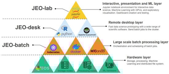
Figure 1.
Graphical representation of BDAP components (Acknowledgement: JRC Big Data Analytics project) [31].
- JEO-desk, a remote data science desktop (based on Ubuntu);
- JEO-batch, a high-performance computing mechanism based on HTCondor;
- JEO-lab, a JupyterLab environment based on a custom Python kernel.
The platform is remotely accessible through a secure and encrypted communication. In addition, critical geospatial data collections (Copernicus and US Geological Survey base and project data) are available in the EOS data-storage file system, developed by the European Organization for Nuclear Research (CERN, from the French “Conseil européen pour la Recherche Nucléaire”) and in collaboration with the JRC, and tested in a pilot installation. It was based on special hardware and designed to meet high requirements, while also being immediately available to the end-user, being easy to use, and having a relatively low acquisition cost [28].
One of the major advantages offered by this platform is the possibility of teleworking—a form of work imposed during the COVID-19 pandemic that may continue in the future [32]. In addition, a decentralized collaboration and support model has been created through which users can share the projects they have developed as well as submit requests to members of the support team.
2.2. Programming Languages—Free and Open-Source Software
One choice made both for the construction of the BDAP platform and for the conduct of the research was the use of free and open-source software (FOSS), as opposed to the proprietary or software-as-a-service (SaaS) solution. The downside of choosing a proprietary or SaaS solution is the risk of vendor lock-in. Vendor lock-in means a business or organization is dependent on a product, service, or software with no ability to replace it with different options due to high transition costs [33]. In addition, research organizations assign to the owner company the right to store, access, analyze, and share their data, with all that implies for their security and confidentiality. The choice of a proprietary and closed-source software (“black box”) platform by an organization would also be in stark contrast to the open-source software strategy 2020–2023 [34] for the promotion of FOSS in the European digital space.
More analytically, for our geo-processing and spatial analysis needs, the GRASS GIS software and its individual modules were used. Spatial information was mapped and visualized using QGIS software, while European Space Agency (ESA) SNAP/gpt software was used to pre-process Sentinel-1 images. In addition, for geo-processing, spatial analysis, visualization, and process automation, bash scripts, and the R and Python programming languages were employed, along with the respective integrated development environments RStudio and Spyder. The job scheduler HTCondor, which creates a high-throughput computing environment, was used for bulk and parallel data processing (Figure 1). Finally, the Geospatial Data Abstraction Library and the specialized library pyjeo [35], created to support the BDAP team, were adopted for image processing, data extraction, and conversion.
3. Main Challenges in Soil Data Processing
The main challenges involved in geo-processing soil big data are (a) developing a framework in which to reproduce the results (reproducibility); (b) harmonizing the different input data (harmonization); (c) merging or mosaicking the high-resolution data parts into a single dataset (compositing); (d) zonally representing and associating statistics (zoning); (e) aggregating the results at different scales; (f) representing maps in geographically coordinated systems; (g) plotting outputs for policy-makers; (h) developing indicators; and (i) developing uncertainty algorithms.
Large-scale processes and datasets on soil erosion, rainfall erosivity, mercury contamination, manure management, and phosphorus are the test cases to address the challenges involved in soil geography.
3.1. Reproducibility—Developing a Software Model Framework for Replicating the Results
The reproducibility of a study refers to the possibility of it being repeated such that, under the same conditions, and using the same data, software, and code, the results are the same. Reproducibility is necessary both for the user conducting the study and wanting to record its procedures and data, and for third parties needing to confirm the findings and their reliability. This should be an easy process that can proceed without mistakes [36].
The need for reproducibility is intensified by the availability of big data and the requirements for its management, pre-processing, and analysis. The rapid availability of big data necessitates a workflow schema that can reproduce the changing standards and results in near real time [37].
To best achieve reproducibility, the processes were automated using R, Python, and bash (where feasible). To ensure consistency and reliability of the results and easy repetition, the sequence of execution steps was recorded using Snakemake software [38]. Snakemake is a workflow engine that provides a readable Python-based workflow-definition language and a powerful execution environment that scales from single-core workstations to computer clusters without modifying the workflow [39].
Apart from ensuring study reproducibility, Snakemake may contribute to the adaptability and transparency of the research project. Soil research is a timeless process that is in constant flux due to the conditions and factors that shape it [40,41]. Using a workflow management system ensures the immediate adjustment or extension of the computing procedures to changing conditions (adaptability), or even a new research process. In addition, the depiction of the workflows and correlations of the individual entities in Snakemake ensures the technical and scientific accuracy of the procedures (transparency). Snakemake offers automation in the form of rules that essentially describe the connections between the procedures through input/output data, to and from each node of the process. These connections are described using a directed acyclic graph.
Software, input data, routine interconnections, and algorithms are components that must be available and documented for the scientific community. For this reason, the distributed version control system Git, and an instance of the GitLab code repository designed by the BDAP team, were used to record the change history, the ability to revert to previous stages of the study, and the need to share code.
For example, the study on phosphorus plant removal from European agricultural land [42] and the improvement of the phosphorus budget in European agricultural soils [43] is a typical form of research in which, due to the large heterogeneity of data and analytical processes, the use of a workflow management system and a scalable approach was particularly important. In addition to the data heterogeneity, a diverse set of software had to be used for data processing, analysis, and presentation. Typically, more than 40 scripts for processing and analyzing data need to be synchronized via a specific execution order. Many times, small changes at one point in the analysis pipeline can produce multiple consequences to the output of other stages of a study. All these procedures were harmonized using adaptions of Snakemake.
3.2. Data Harmonization
The heterogeneous volume of big data, in terms of source, geometry, resolution, and semiology, requires harmonization. Data harmonization is a process in which heterogeneous datasets are transformed in such a way that they become unified, homogeneous, and compatible so that they are comparable to each other [44,45]. A variety of techniques have been developed over time for big data harmonization [46,47].
The development of merging methodologies, scales, and heterogeneity in remote-sensing data allows data fusion on a global scale [48]. At the European level, harmonization models have been developed for geospatial data to be made compatible with the European INSPIRE Directive [49]. More specialized models for soil data have been developed for harmonization at both the global [50,51] and European scales [52,53].
In our case, the harmonization required focused on the spatial, temporal, and descriptive information of the data. Spatial data at various resolutions were merged into single sets in order to render the information to the appropriate spatial unit. The descriptive information, respectively, had to be identified with the merging of the data in the respective spatial hierarchy.
A typical example of data harmonization involved the development of the phosphorus budget for European agricultural soils [43], where production data per crop from the Common Agricultural Policy Regionalized Impact (CAPRI) model had to be merged and adapted in order to fit the administrative units (regions) of the EU. This harmonization was not only about spatial integration, but also hierarchical identification in predefined categories of information. The inputs for the phosphorus originated from fertilizers, manure, chemical weathering, and atmospheric deposition, and the outputs were from uptake by plants, plant residues, and erosion, and so repartition methods were required to appropriately attribute the spatial distribution of phosphorus to all the necessary spatial levels (country—nomenclature of territorial units for statistics (nomenclature des unités territoriales statistiques, NUTS) Level 0, regions—NUTS Level 2). The NUTS were created by Eurostat and represent the official, hierarchical, geographical divisions of the EU for regional statistics. Data harmonization was also applied on a timescale where monthly or annual data were merged into higher time units (decades or time frames of 5 years). For example, during the assessment of phosphorus fertilization uncertainty at the country level, the input data were averaged for the years 2011–2019.
3.3. Compositing—Merging or Mosaicking High-Resolution Data Parts into a Single Dataset
Composites or mosaics are common techniques used in GIS and remote sensing for merging spatial data [54,55]. In GIS, mosaicking is a process in which a single spatial dataset is created by combining several individual, usually adjacent, rasters. Gaps that can occur during mosaicking receive a nodata value. During the compositing process, spatially overlapping rasters are merged into one file. The values of each pixel in this generated file result from applying a function to the individual raster pixels (mean, median, standard deviation, minimum, maximum, sum, etc.). Sometimes, compositing means the creation of a single multiband raster from individual rasters. In this case, no function is applied, but each raster becomes a separate band in the output raster.
For example, the global rainfall erosivity projections for 2050 and 2070 [56] apply a worldwide mean standard deviation to 19 general climate models for three different Representative Concentration Pathways (RCPs) scenarios of Coupled Model Intercomparison Project model 5 (CMIP5). In such cases, the use of JEO-batch services, the high-throughput computing environment of HTCondor (Figure 1), and the tiling mechanism offered by the pyjeo library were particularly useful in compositing global maps in a reasonable time and in an efficient way. The number of files per year (51), the global coverage of the maps, and the high spatial resolution (~1 km) rendered the production of this data process practically impossible using typical computational systems due to their limited resources. Raster compositing was one solution. An alternative option was the tiling mechanisms offered by the pyjeo library, which implies that files are fragmented through an out-of-the-box mechanism on smaller pieces based on a grid. For every grid, the mean composite process was executed separately and in parallel through the HTCondor distributed mechanism. Then, the output files from each subset were joined together to form a new final output file. This procedure makes feasible the timely, effective, and computable merging of large geospatial datasets.
3.4. Zoning—Producing Aggregated Statistics
Another common practice for analyzing and visualizing variables and indicators with a spatial dimension is zonal statistics. Zonal statistics are executed in raster files with accompanying zone (either raster or vector) files. During the process, for each zone, a function (e.g., mean, median, and minimum) is applied to the raster. The necessity for using such a method for big geospatial data led to the development of innovative zonal statistics calculation methods with parallel and distributed processing. This requires the use of graphics processing units, with global application, and for data with a petabyte order of magnitude [57,58].
When presenting the results of zonal statistics, the effect of the modifiable areal unit problem (MAUP) requires special interpretation. The term “MAUP” was first coined by Openshaw and Taylor [59] who assessed the effect of differentiating space delimitation or reconstitution into new distinct spatial units on output data and results. The first case concerned the “problem of zones”, which does not change the number of partition zones of the space, but rather their boundaries, shapes, and positions. The second property is the “scale problem”, which arises through the aggregation (or disassembly) of spatial units or by changing the resolution of the data. Both cases can lead to inconsistencies in the research results.
Zonal statistics are commonly used in the context of soil research in ESDAC for aggregating data, developing indicators, drawing conclusions, and highlighting spatial differences at the European level. An example of this method is the soil loss from river basins (Figure 2). The method vividly depicts the spatial distribution of indicators in space and provides the possibility to compare data per spatial statistical unit (Figure 2). Detail is lacking when assembling a polygon, but by using zonal statistics, the noise is reduced and the necessary generalizations are ensured. However, modifying or scaling polygon shapes can lead to different results. Particular attention needs to be paid to the stages of the study that are affected by the MAUP because the impact of the problem can be vital [60,61]. Choropleth maps (using MAUP as a tool) can manipulate the reader [62,63] and be used as a means of misinformation in processes that are not related to the scientific methodology, but rather to political propaganda.
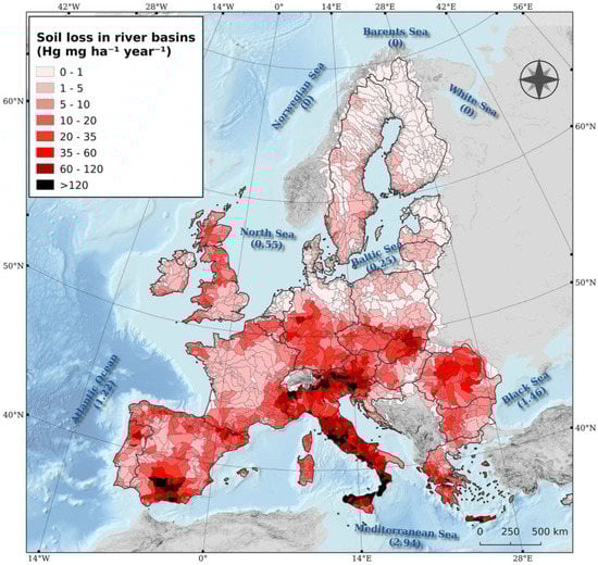
Figure 2.
Estimated Hg losses to river basins and Hg fluxes to sea outlets (Mg yr−1) due to water erosion [64].
River basin boundaries are attributed through geomorphological processes and, consequently, no anthropogenic/human intervention is involved. In addition, NUTS statistical units are the commonly accepted administrative boundaries, widely established at the European level. The map symbols are ideologically/politically neutral and represent only the actual conceptual content, quality, or quantity of the variables they symbolize. Data insights are achieved by choosing the appropriate classification method and meaningful class breaks across the entire data range. The goal is to highlight the differences in the studied attribute (e.g., mercury loss) by choosing the best possible classification method (quantile, equal interval, natural breaks, or custom).
3.5. Spatial Resolution—Aggregating Results at Different Scales
Choosing the right scale for data representation is crucial in soil geography. The generalized image offered at the small scale can obscure details and relationships at the micro level. However, even a large-scale map can add noise and highlight structures that are of no use to the purpose of the study. The selection of spatial resolution depends on the phenomenon that is under investigation, and it is therefore quite legitimate to change the cartographic scale. Over time, even before the advent of GIS and digital mapping, soil research was largely bound by the static scale of proxy variables (such as climate, vegetation, and topography) and the inability to dynamically define the scale of the topic under investigation [65]. Nowadays, digital technology provides the option to evaluate the appropriate scale of the work and to adapt to every eventuality.
The spatial resolution of a study is defined and interpreted in direct relation to the scale of the map. At global scales, low-spatial-resolution mapping, country-level visualization, or large bioclimatic zones make sense, as more detail adds noise and hides potential spatial patterns. On the other hand, European-scale research can be attributed to smaller geographical reference units (e.g., NUTS2 or catchments) or high cell resolution to ensure that cartographic generalization does not remove valuable information.
For example, in the global rainfall erosivity projections for 2050 and 2070 [56], the mapping was performed at the optimal global-scale resolution to ensure the differences in erosivity patterns were apparent without adding unnecessary noise (Figure 3). For the study on mercury losses in European topsoils [64], the mapping scale was European and the reference unit was the river basin because this drove the process of sediment flow (Figure 4).
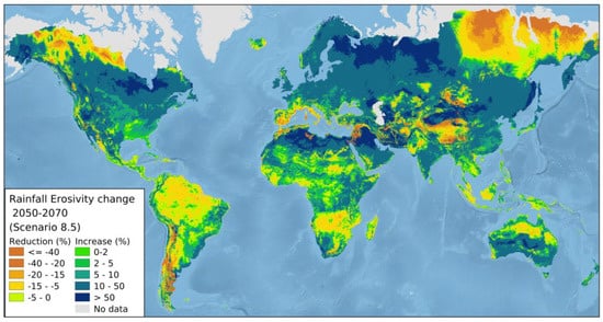
Figure 3.
Erosivity projections for the period 2050−2070 for the scenario RCP 8.5 [56].
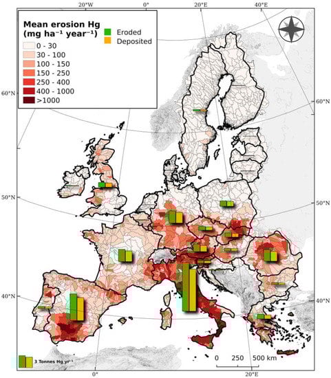
Figure 4.
Estimated Hg displaced with water erosion per catchment [64].
Different visual approaches are also available, aimed at facilitating the end-user and providing cartographic elegance. An innovative cartographic presentation is given in Figure 5 where the values are presented on a hexagon grid map at a 250 km2 spatial resolution, a scale different to that of the primary data. On this map, the objective was to highlight the degree of agreement in trends of rainfall erosivity using several climate-change prediction models for 2050. Having 250 km2 cell dimensions ensured a balance between the generalization of the information and the preservation of the variability.
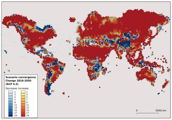
Figure 5.
Scenario convergence aggregated a pixel of 250 km2. Each scenario counts as +1 (increase) or −1 (decrease). Each pixel represents the sum of the increased/decreased scenarios [56].
3.6. Cartography—Map Projections
The study of soil-related spatial phenomena at the European and global scales requires different geographic reference systems. The reference system is chosen not only on the basis of cartographic performance, but also on the spatial analysis because each projection system brings about changes in attributes, such as distances, angles, and areas. As early as 1999, at a conference organized by the JRC and the Multi-purpose European Ground Related Information Network, it was jointly agreed that the most appropriate reference system is the European Terrestrial Reference System 89 (ETRS89) [66]. The ETRS89 was adopted in 1990 in Firenze [67]. It uses the Geodetic Reference System 1980 ellipsoid as its reference ellipsoid, the geometric center of the ellipsoid being coincident with the center of the mass of the earth and the origin of the coordinate system. Thus, in the context of studies on the analysis and visualization of data at the European scale, the geographical reference system ETRS89 is used (Figure 6), which is suitable for mapping at all scales and for the preservation of distances and areas.
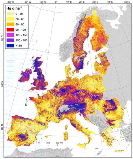
Figure 6.
Hg stock (g ha−1) in European topsoils [64].
In order to visualize datasets on global maps, the World Geodetic System (WGS) 84 was projected onto a plate carée projection (i.e., Figure 3). The WGS 84 is an earth-centered, earth-fixed terrestrial reference system and geodetic datum. It comprises a set of constants and model parameters (geoid, reference ellipsoid, a standard coordinate system, and altitude data) that describe the earth’s size, shape, gravity, and geomagnetic fields. The WGS 84 is the standard US Department of Defense definition of a global reference system for geospatial information and is the reference system that underpins the Global Positioning System [68]. It is compatible with the International Terrestrial Reference System, which is maintained by the International Earth Rotation and Reference Systems Service.
The plate carrée map projection is a simple equidistant cylindrical projection. Its meridians and parallels are straight lines that outline squares from east to west and north to south. Due to its simplicity, WGS 84 has been a very common projection, especially during the 15th and 16th centuries. The plate carrée projection has the standard parallel at the equator [69]. One of its main disadvantages involves its distortions of shapes and areas. Because of the distortions introduced by this projection (Figure 7a), it is not used for navigation or cadastral mapping, but it is very common in thematic mapping, GIS, and global raster datasets (i.e., Celestia and NASA World Wind) [70]. The plate carrée projection ignores the earth’s curvature because it assumes that there is a linear relationship between the projection of a geographic point (φ, λ) into Cartesian coordinates (x, y).
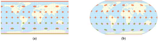
Figure 7.
Tissot’s Indicatrix depicting the distortions for (a) plate carrée and (b) Robinson pseudo-cylindrical projection (Acknowledgement: Justin Kunimune) [72,73].
In some cases, in order to create more visually appealing global maps, the Robinson pseudo-cylindrical projection was used (see example in Figure 8). This is a pseudo-cylindrical projection, with the standard parallel at the Equator. It has the same distortions as the Mercator projection. Thus, between about 0 and 15°, the areas and shapes are well preserved, whereas, from approximately 15° north and south to approximately 45° north and south (Figure 7b), there is an expansion of the acceptable distortion. In polar regions, the distortions are less pronounced. Its main advantage is the pleasing appearance, but with the disadvantage of increased distortions. The Robinson projection is neither equal-area, conformal, equidistant, nor true in direction [71]. The distortions introduced by the plate carrée and Robinson pseudo-cylindrical projection are presented in Tissot’s Indicatrix (Figure 7) [72,73]. The Tissot’s Indicatrix method was introduced in 1859 by Nicolas Auguste Tissot, a French mathematician, in order to visualize local distortions caused by map projections.
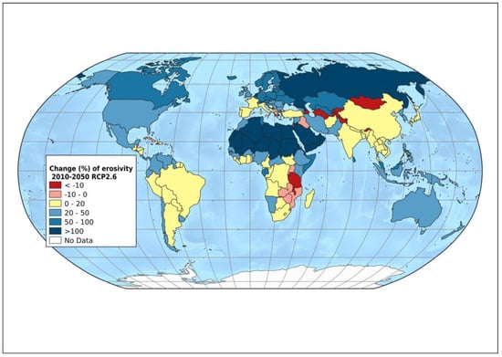
Figure 8.
Change (%) of erosivity of the period 2010−2050 for the scenario RCP2.6 [56].
3.7. Presentation—Plotting Outputs in a Comprehensive Way
In the context of better communicating the research results, waterfall charts, pie charts (Figure 9), donut charts, box plots (Figure 10), and dumbbell plots (Figure 11) were produced. In many cases, the maps were combined with plots to provide a more comprehensive picture of the results.
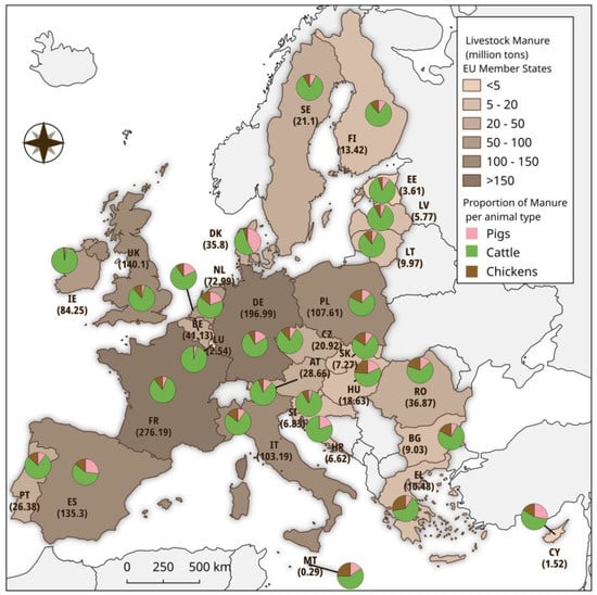
Figure 9.
Annual manure production (million tonnes) in the European Union and UK and distribution according to main animal types (period: 2016–2019) [74].
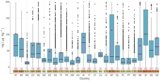
Figure 10.
Mercury (Hg) concentration per country as μg Kg−1 [64].
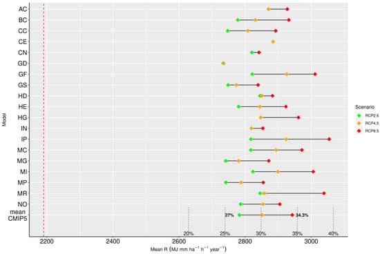
Figure 11.
The range of model predictions for years 2050 and 2070 [56].
Waterfall charts are a special category of bar plots that depict how an initial value is changed as new values are successively added (or deducted). Its name comes from its characteristic “waterfall” appearance. The advantage to the end-user is not only being able to ascertain the initial and final values of a size, but also the entire accompanying record that had an effect in the intermediate stage. The initial bar is defined on the basis of a baseline, with the next bar using the end of the previous bar as the baseline. This difference in the baseline is also one of the weaknesses that can disorient the end-user. In addition, disproportionate changes per stage (bar) result in some bars being very small and unreadable and some being very large.
In other cases, it is necessary to present the proportions by data group. Pie charts are used to depict these proportions as parts of a circle. A representative example of using pie charts in combination with a map is given in Figure 9, in which the pie charts correspond to each country. Each pie chart depicts the proportion of manure per animal type. Although no particular explanation is needed for the end-user, pie charts are less readable when incorporating the proportions of several groups. Moreover, they do not present the absolute values per group and they do not show inter-temporal changes; therefore, comparisons between pie charts are not easy. A variant of the pie chart is the donut chart. In fact, this is a pie chart with a hole in the middle. This hole is usually a space for including additional information, such as labels. They have more restricted possibilities because they are intended for only a few (2–4) groups of data.
A visualization method used to describe and compare the distributions of several variables and groups is the box plot. These briefly and graphically attribute a variable distribution because they show the median, first, and third quarters of the data (lower and upper hinges), with whiskers that extend from each hinge to 1.5 times the interquartile range. Any data values that exceed the whisker limits are considered to be outliers and are provided as a point on the graph. A typical example of a box plot, used for comparing distributions, is shown in Figure 10. In that plot, mercury concentrations are expressed per country. This characterizes the potential of the box plot to compare the distributions of this variable, with even a limited plot being able to express a number of descriptive statistical measures.
Box plots, on one hand, provide brief information; although, on the other hand, they conceal other important information on the distribution of the data (e.g., the number of observations). For this reason, in Figure 10, further descriptive measures have been included, such as the average, the number of samples with high mercury concentrations >200 µg kg−1, and the percentage proportion of high-concentration samples compared to the total number per country.
Finally, a series of dumbbell plots were used to represent differences through time and to emphasize deviations in the estimates of individual models. These offer very comprehensive visualizations of deviations and are therefore used to compare multiple data groups. A typical example of a dumbbell plot is provided in Figure 11. This refers to the comparison of predictions of future rainfall erosivity for 2070 based on climate-change scenarios RCP2.6, RCP4.5, and RCP8.5 from the CMIP5 prediction model.
Another option to provide comprehensible information to the end-user is through intricate maps; for example, the phosphorus budget at NUTS Level 0 on a choropleth map (Figure 12). Along with the color grading representing the phosphorus budget, the labels provide summary information on the phosphorus inputs and outputs, and the uncertainty at the 90% confidence level. The choice of color scheme type (discrete or continuous) is not accidental. Color schemes are a series of associated colors that correspond to certain values. There are two methods that cover the construction of color schemes.
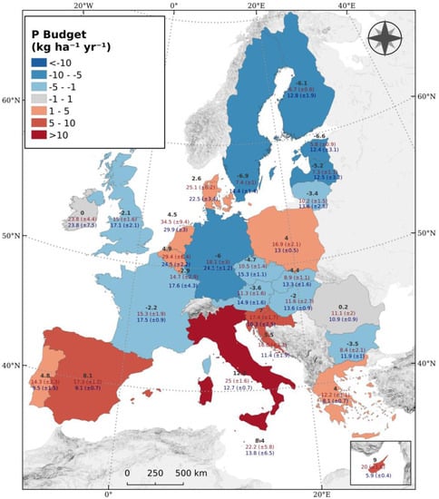
Figure 12.
Phosphorus budget at country scale including sum of inputs/outputs and uncertainties [43].
The first is the continuous-gradient method, where the maximum and minimum values correspond to two distinct colors, and the intermediate values are defined, through an interpolation method, as a mix of these two colors. The continuous-gradient color scheme represents the full range of dataset values with greater success. However, the continuous gradient may be influenced by outliers where the data are skewed. In addition, it is not possible for the human eye to accurately match each color to its corresponding value, especially when no linear interpolation of the color scale is used. For these reasons, discrete color schemes are mainly used to create maps.
The second method—the discrete color scheme—consists of a series of distinct colors. These are usually successive shades of one color. Each distinct color corresponds to a specific range of data values. Although details of the data are partially lost, spatial patterns are better depicted and comparisons between cases are easier to see. The end-user can clearly match the color on the map or diagram with the corresponding value range in the legend. As an extension of this method, diverging color schemes can also be used. These involve a discrete color scheme with a light color in the middle and two different dark colors at the ends that converge toward the center of the palette. This scheme is mainly used where there is a need to distinguish positive and negative values or, more generally, where there is a divergence in data values from a central/neutral point of convergence. A representative example of the discrete color scheme is given in Figure 12. The third type of color scheme is the categorical color scheme. This is made for simple visual distinction/categorization, where the color does not correspond to any value or type of hierarchy.
Maps and charts are produced with the aim of delivering the actual distribution of the data to the end-user in the most optimal way. In addition to the choice of color scheme (continuous or discrete), the interpolation of the color scale method is also important. During the interpolation process, all data values are attached/assigned to one color. The most common color interpolations are the linear, quantile, natural break, pretty break, logarithmic scale, and standard deviation styles. In many cases, if linear interpolation of the color scale is selected and there are outliers, important details of the data distribution can be lost.
Finally, with respect to choropleth maps, the values need to be standardized over a unit area (usually a hectare or square kilometer). If absolute values are used, then there is a risk of large-area polygons also summing up to high values.
In other cases, it may be deemed necessary to combine the cartographic information with diagrams; Figure 9 shows the quantity of livestock manure per EU Member State in combination with the proportion of manure per animal type.
The results of this study, in addition to the scientific publications that emanated from it, have been disseminated as open data through the ESDAC (https://esdac.jrc.ec.europa.eu/, accessed on 30 September 2022).
3.8. Statistics—Developing Indicators
Appropriate insights into soil properties, and the threats to and functions of these, through their spatial distributions, contribute to their proper management and mitigation in the case of land degradation. This is important in the context of developing indicators and trends in order to better support soil-relevant policies, such as the Soil Strategy 2030, the Common Agricultural Policy (CAP), the Farm-to-Fork Strategy, and the Zero Pollution Action Plan [75,76].
Examples of policy-relevant indicators are the mean soil erosion rate and the share of agricultural area under severe erosion used to evaluate the environmental performance of the CAP [77]. By using a bar plot (Figure 13), the output of the study is presented for the assessment of soil loss by water erosion in the EU [77] as an estimated rate per country for the years 2000, 2010, and 2016.
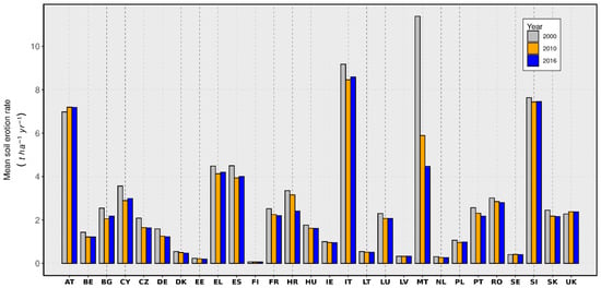
Figure 13.
Estimated mean soil erosion rate per country.
The EU Soil Observatory (EUSO) intends to host a dashboard with indicators monitoring soil health in the EU. The EUSO was launched in December 2020, and its main aim is to disseminate data and knowledge about soil protection to the wider scientific community and policymakers, to support research, and to contribute to public awareness regarding soil protection [76]. The EUSO dashboard will host a series of periodically updated indicators that will contribute to the assessment of soil-protection policies. Currently, the core of the EUSO—the ESDAC—hosts harmonized datasets that assess soil conditions in the EU. The ESDAC includes, among other things, pan-European datasets for soil organic carbon, soil erosion, nutrients, diffuse contamination, soil biodiversity, and soil physical/chemical properties. Some of these harmonized datasets have been used in the context of the new EU Soil Strategy, the CAP, the Zero-Pollution Action Plan, and the EU’s Sustainable Development Goals (SDGs).
3.9. Uncertainty
A common way to evaluate uncertainties in modeling outputs is the Monte Carlo method. This method is widely used in the scientific fields of biology, engineering, geophysics, meteorology, information technology, public health, and commerce. With the Monte Carlo method, one or more variables are represented by a probability distribution function, and a large number (hundreds or thousands) of random values from this distribution are extracted by sampling. The resulting values from these iterations provide a probability distribution of this variable [78]. The method is widespread in soil science, with applications focusing on soil moisture [79], heavy-metal contamination [80], landslide susceptibility and hazard assessment [81], and soil classification and stratification [82].
The Monte Carlo method was also used in the study on phosphorus plant removal from European agricultural land [42] and the improvement of the phosphorus budget in European agricultural soils [43]. In specific, Monte Carlo was used to estimate the uncertainty in phosphorus plant removal as a result of the heterogeneity in crop production, humidity rates, and the phosphorus concentration in plant tissues. A total of 1000 Monte Carlo simulations were performed for each cropping system and NUTS Level 2 region. The outputs of these Monte Carlo simulations resulted in a standard deviation for phosphorus plant uptake at both the regional and national scales with a 90% confidence level.
4. Discussion
This article presented the methods, techniques, tools, and infrastructure used in soil research to geo-process large-scale datasets at the ESDAC. This could be used as a guide for the processing, analysis, and presentation of (large) geospatial soil data. The rapid disposal of geographical and remote-sensing data requires an approach that exceeds the capabilities of standard computing systems. The JRC is a successful example of how adopting and implementing innovative and powerful computing systems, interdisciplinary cooperation, and effective data management can be applied. End-users and organizations can now be made aware that there are high-performing computational systems capable of implementing the geo-processing of large spatial data in reasonable timeframes.
The approach to this new era of large data is not only limited to technological adaptations, but also includes a change in the model of collaboration through remote access. In this case, the new norm of teleworking provides a novel opening for cooperation among scientists through online points of collaboration and support (e.g., GitLab) via teleworking capabilities (JEO-desk).
The adoption of FOSS as another new norm is a huge advancement for open and collaborative research. It has now been confirmed that the use of FOSS is not a risk to research, but a choice tried and tested by a high-level research organization. In addition to the economic benefits, FOSS ensures the transparency of its algorithms and the independence of research beyond the decisions of private companies. With this option, the possibility of vendor lock-in, or a company handing research data and their security to the private sector, is excluded. The removal of high-cost software licenses for proprietary software will result in enormous savings that can be used for new scientific staff assignments and other research processes.
Specific criteria have been presented here that clarify how to choose a map projection for pan-European or global geospatial data, and how to use the appropriate color scheme and classification method to highlight spatial patterns. In addition, attention has been drawn to the endogenous weaknesses (projection distortions, MAUP) in the cartographic process in such a way that the future user can avoid failures and misinterpretations of their research results.
Geospatial data were harmonized into uniform spatial entities using identical standards and characteristics (coordinate reference system, units of measurement, spatial resolution, and cartographic symbols), regardless of the properties of the primary sources. Harmonization is necessary for temporal resolution where detailed temporal scales are reduced to coarser units so as to generate uniform time series. This methodology makes it possible to compare heterogeneous data on a European or global scale.
Emphasis is given to making the results interpretable to the broader scientific community. For this reason, a series of charts and maps were used to describe divergences, aggregations, distributions, and proportions in a comprehensible manner. ESDAC stands as the main, high-traffic distribution center of high-quality datasets for the state of soils at the European level with 10,000 data downloads in 2022 [30]. It is worth mentioning that the distributed datasets are available with specific standards (and metadata) that describe the format, the conceptual content, the units of measurement, the coordinate reference system, and the accompanying publications in scientific journals for the end-user. In addition, proposals have been made on how the users could handle the uncertainty in environmental indicators through the Monte Carlo method. Its practical application and utility have been concisely exemplified.
At the level of improvisation and data aggregation, current research has developed (see the phosphorus budget) and adapted indicators from other sciences (i.e., the Lorenz curve) to the needs of soil science. For example, Bezak et al. [83] investigate the use of the Lorenz curve in rainstorm frequency and Gini coefficients in measuring the inequality of storm events.
Despite the comprehensive effort to manage large-scale data, there is still room for improvement. The digital environment for the management and processing of geospatial soil data remains classified and available only to JRC researchers with no potential for detailed analysis by the wider scientific community. However, users and organizations in close collaboration with JRC researchers do have access to the data computing facilities.
Recent works in the field of geoinformatics and earth observation have necessitated that common data analysis (not just consumption) could be a public good from all scientists [84,85]. The Copernicus Open Access Hub [86] has been cited as an example of a geospatial platform for sharing not only data, but also computing resources, technical infrastructure, and algorithms. This integrated research environment aims also to exploit the vast amounts of data available from the wider scientific community.
In the case of the ESDAC, however, data-sharing is one-dimensional, with the provision of static files. In future efforts to upgrade the ESDAC infrastructure, it is proposed to make geospatial data more easily accessible to the public through various services (webmapping, application programming interfaces (APIs), fast processing algorithms, distributed computing, and cloud applications for wider audiences).
The goal is to develop an API suitable for large-scale spatial deployments that will allow users to connect and download data in a standardized way from cloud platforms and data cube services [87]. The API will allow the immediate availability of data in a homogenized form and their integration into programming environments for modeling and analysis. It can be further separated into more specialized parts that will provide Catalog API, Statistical API, and Processing API according to the Sentinel Hub implementation [88]. The basic infrastructure—BDAP [28]—which can support this goal already exists within the organization.
However, the significant efforts made by the JRC, through the adoption of BDAP and the support of open-source software, should not be overlooked. The use of the BDAP platform opens new horizons for the management, processing, and analysis of soil data. The adequate storage and computing resources provide possibilities for investigating, in a timely manner, research questions at high spatial resolutions, at the European and global levels, and on a long-term basis. This feature is not available with standard computer systems or in organizations with limited computing resources. At the same time, the results of this research have been disseminated both through publications and the relevant web portals, which can be viewed as reference points for science. The research results have been presented in such a way (via diagrams, maps, figures, tables, etc.) that they are easily accessible by a wide scientific audience (undergraduate and PhD students, academics) and end-users (policymakers).
Recently, the technical capacity for developing dynamic dashboards via a Jupyter extension—Voila—has been developed. Viola allows the conversion of Jupyter Notebooks to standalone web applications. These dashboards are, for the time being, accessible only to JRC members, but they represent an important tool for the decision-making processes of policymakers. They have the advantage of allowing the presentation of data as web maps, diagrams, and tables in live and dynamic ways. In addition, one of the most important advantages of Voila is that it can provide data analysts with the potential to build web applications using tools known to them (such as Python), not having to use web-specific languages (HTM, JavaScript, etc.). In this way, for the data analysts, the presentation of research results to policymakers is facilitated and accelerated. Another option for obtaining deeper data insights and disseminating information to the wider scientific audience is the adoption of Qlik. Qlik is a cloud platform for real-time analytics, data warehouse automation, visualization, and data dashboards.
In addition, the choice of using FOSS to conduct research is essentially an admission that scientific knowledge must be independent of business practices that impose limited access on algorithms, which run the risk of vendor lock-ins, and deprive valuable scientific staff of jobs due to the financial costs of these. Because research results provide scientific evidence for policy proposals and broader strategic planning, the transparency of algorithms and workflows (as opposed to proprietary “black boxes”) at all stages of research is a critical factor. Those directly affected by the accompanying policies and planning should have the right to access the underlying process. In fact, with the advent of big (spatial) data and the participation of more and more partners worldwide, checking the reliability of the research is becoming even more difficult than in the past. The transition to open science and open data has been a significant realization in recent years [89].
On the other hand, although there is a plethora of free software repositories in the world of open source, the relevant section of the JRC that focuses on soil research lags behind in publishing code related to workflows, models, and their related documentation for the complete reproduction of their research results. The factors that limit code disclosure may be related to copyright issues, its degree of completeness and accuracy, the complexity and heterogeneity of the data, and the obligation to support and educate the public, as well as the scientific community [90].
Reproducible research initiatives in the scientific community have already begun in the field of publication. For example, the publishers of the journals Scientific Data (http://www.nature.com/sdata/, accessed on 15 June 2022), from the Nature Publishing Group, and Toxicological Sciences, in collaboration with the Dryad Digital Repository, Elsevier, and GitHub, have taken action to ensure that the contents of their publications will be accompanied by the corresponding code [91]. A similar discussion has been initialized in the field of remote sensing, for which a specialized journal [92] has been proposed.
The ESDAC follows and adapts the current evolutionary process—sometimes referred to as data science, open science, big data, or spatial analytics. Methodologically, soil science, as applied to the JRC, merges a variety of techniques, but now requires the exploitation of vast and varied spatial data based on openness, transparency, sharing, and reproducibility.
5. Conclusions and Future Developments
Soil is inextricably linked to the concept of space and soil research is inseparable from this concept. New technologies and remote sensing offer novel possibilities in the study of soil properties and phenomena at various spatial scales. New challenges and opportunities have arisen with the availability of big data. At the same time, innovative management and analysis techniques have been developed. The JRC has adapted to the spirit of this new era by evolving pioneering research tools and methodologies aimed at exploiting these conditions and effectively disseminating research outputs to the scientific community.
Future plans include the use of new tools and techniques (large-scale batch processing and machine/deep-learning infrastructure) to exploit research advancements in geo-processing billions of objects (such as parcels), including soil-property values. There is a plan to calculate a series of soil-erosion, soil organic carbon, pH, and nutrient indicators for ~70 to 75 million parcels, corresponding to the entire (~160 million ha) agricultural area of the EU countries. This research is becoming especially important because it will provide a detailed account of the state of the land that has been subjected to intensive exploitation. The fragmentation of agricultural land into multiple agricultural parcels has changed its potential for intensive use. In France and Austria, agricultural land has been fragmented into averages of 22 and 37 parcels/km2, respectively. In Cyprus, Slovenia, and Italy, the fragmentation of agricultural land is even greater as the landscape is dominated by much smaller parcels of 215, 119, and 117 parcels/km2, respectively. This variety of agricultural land fragmentation exerts variable impacts on the soil of the respective parcels. New spatial patterns that affect the properties of the ground in different ways are expected to be revealed, based on the number of parcels per unit of surface area. In addition, temporal changes in the density and sizes of the parcels per unit surface area may not only indicate changes in the management conditions and exploitation of the agricultural land, but also may result from land-use changes (pressures of urban sprawl, forest expansion, changes in production models, etc.).
In addition, new information and communication technologies are proposed for the future, with plans for data sharing through web-map services, and a map viewer for navigation and the direct visualization of geospatial data. The above technologies will be structured according to both the INSPIRE Directive and international interoperability standards (Open Geospatial Consortium). Data sharing will be extended to integrated interoperability systems, APIs, and big earth-observation data management and analysis platforms.
An integral part of the transition to the new scientific reality is the need for an interdisciplinary approach to territorial phenomena. Close cooperation and consultation between individual scientific partners will be required for the analysis of complex questions. This interdisciplinary community of soil scientists, information technology experts, modelers, geographers, environmental scientists, and data managers will merge their various scientific findings under the evolving umbrella of geography.
Author Contributions
Conceptualization, L.L. and P.P.; methodology, L.L. and P.P.; software, L.L.; validation, L.L.; formal analysis, L.L.; investigation, L.L.; resources, P.P.; data curation, L.L.; writing—original draft preparation, L.L.; writing—review and editing, L.L. and P.P.; visualization, L.L.; supervision, P.P.; project administration, P.P. All authors have read and agreed to the published version of the manuscript.
Funding
This research received no external funding.
Data Availability Statement
The study is based on data and maps that have been already available in the European Soil Data Centre (https://esdac.jrc.ec.europa.eu/resource-type/datasets) (accessed on 16 September 2022).
Conflicts of Interest
The authors declare no conflict of interest.
References
- Brevik, E.C.; Homburg, J.A.; Sandor, J.A. Soils, Climate, and Ancient Civilizations. In Developments in Soil Science; Elsevier: Amsterdam, The Netherlands, 2018; Volume 35, pp. 1–28. ISBN 978-0-444-63950-9. [Google Scholar]
- Moskal-del Hoyo, M.; Lityńska-Zając, M.; Korczyńska, M.; Cywa, K.; Kienlin, T.L.; Cappenberg, K. Plants and Environment: Results of Archaeobotanical Research of the Bronze Age Settlements in the Carpathian Foothills in Poland. J. Archaeol. Sci. 2015, 53, 426–444. [Google Scholar] [CrossRef]
- Perlès, C.; Monthel, G. The Early Neolithic in Greece: The First Farming Communities in Europe, 1st ed.; Cambridge University Press: Cambridge, UK, 2001; ISBN 978-0-521-80181-2. [Google Scholar]
- Tan, B.; Wang, H.; Wang, X.; Yi, S.; Zhou, J.; Ma, C.; Dai, X. The Study of Early Human Settlement Preference and Settlement Prediction in Xinjiang, China. Sci. Rep. 2022, 12, 5072. [Google Scholar] [CrossRef] [PubMed]
- Beach, T.; Dunning, N.; Luzzadder-Beach, S.; Cook, D.E.; Lohse, J. Impacts of the Ancient Maya on Soils and Soil Erosion in the Central Maya Lowlands. CATENA 2006, 65, 166–178. [Google Scholar] [CrossRef]
- Ford, A.; Clarke, K.C.; Raines, G. Modeling Settlement Patterns of the Late Classic Maya Civilization with Bayesian Methods and Geographic Information Systems. Ann. Assoc. Am. Geogr. 2009, 99, 496–520. [Google Scholar] [CrossRef]
- Rodrigo-Comino, J.; Senciales, J.M.; Cerdà, A.; Brevik, E.C. The Multidisciplinary Origin of Soil Geography: A Review. Earth-Sci. Rev. 2018, 177, 114–123. [Google Scholar] [CrossRef]
- Miller, B.A.; Brevik, E.C.; Pereira, P.; Schaetzl, R.J. Progress in Soil Geography I: Reinvigoration. Prog. Phys. Geogr. Earth Environ. 2019, 43, 827–854. [Google Scholar] [CrossRef]
- Carre, F.; Krasilnikov, P.; Montanarella, L.; European Commission; Joint Research Centre; Institute for Environment and Sustainability. Soil Geography and Geostatistics Concepts and Applications; Publications Office: Luxembourg, 2008. [Google Scholar]
- Needham, B.; Louw, E.; Metzemakers, P. An Economic Theory for Industrial Land Policy. Land Use Policy 2013, 33, 227–234. [Google Scholar] [CrossRef]
- Weber, A. Theory of the Location of Industries/Alfred Weber; Translated with an Introduction and Notes by Carl J. Friedrich. In Theory of the Location of Industries; University of Chicago Press: Chicago, IL, USA, 1929. [Google Scholar]
- Mason, G. Land as a Distinctive Factor of Production. Available online: http://www.wealthandwant.com/docs/Gaffney_LaaDFoP.html#A-1 (accessed on 28 April 2022).
- El-Barmelgy, M.; Shalaby, A.; Nassar, U.; Ali, S. Economic Land Use Theory and Land Value in Value Model. Int. J. Econ. Stat. 2014, 2, 91–98. [Google Scholar]
- Mazúr, E. Space in Geography. GeoJournal 1983, 7, 139–143. [Google Scholar] [CrossRef]
- Angelopoulou, T.; Tziolas, N.; Balafoutis, A.; Zalidis, G.; Bochtis, D. Remote Sensing Techniques for Soil Organic Carbon Estimation: A Review. Remote Sens. 2019, 11, 676. [Google Scholar] [CrossRef]
- Babaeian, E.; Sadeghi, M.; Jones, S.B.; Montzka, C.; Vereecken, H.; Tuller, M. Ground, Proximal, and Satellite Remote Sensing of Soil Moisture. Rev. Geophys. 2019, 57, 530–616. [Google Scholar] [CrossRef]
- Chabrillat, S.; Ben-Dor, E.; Cierniewski, J.; Gomez, C.; Schmid, T.; van Wesemael, B. Imaging Spectroscopy for Soil Mapping and Monitoring. Surv. Geophys. 2019, 40, 361–399. [Google Scholar] [CrossRef]
- Ballabio, C.; Lugato, E.; Fernández-Ugalde, O.; Orgiazzi, A.; Jones, A.; Borrelli, P.; Montanarella, L.; Panagos, P. Mapping LUCAS Topsoil Chemical Properties at European Scale Using Gaussian Process Regression. Geoderma 2019, 355, 113912. [Google Scholar] [CrossRef]
- Pham, B.T.; Nguyen, M.D.; Bui, K.-T.T.; Prakash, I.; Chapi, K.; Bui, D.T. A Novel Artificial Intelligence Approach Based on Multi-Layer Perceptron Neural Network and Biogeography-Based Optimization for Predicting Coefficient of Consolidation of Soil. CATENA 2019, 173, 302–311. [Google Scholar] [CrossRef]
- Padarian, J.; Minasny, B.; McBratney, A.B. Machine Learning and Soil Sciences: A Review Aided by Machine Learning Tools. Soil 2020, 6, 35–52. [Google Scholar] [CrossRef]
- Campbell, J.B.; Wynne, R.H. Introduction to Remote Sensing, 5th ed.; Guilford Press: New York, NY, USA, 2011; ISBN 978-1-60918-176-5. [Google Scholar]
- Mohanty, B.P.; Cosh, M.H.; Lakshmi, V.; Montzka, C. Soil Moisture Remote Sensing: State-of-the-Science. Vadose Zone J. 2017, 16, vzj2016.10.0105. [Google Scholar] [CrossRef]
- Peng, J.; Biswas, A.; Jiang, Q.; Zhao, R.; Hu, J.; Hu, B.; Shi, Z. Estimating Soil Salinity from Remote Sensing and Terrain Data in Southern Xinjiang Province, China. Geoderma 2019, 337, 1309–1319. [Google Scholar] [CrossRef]
- Aiello, A.; Adamo, M.; Canora, F. Remote Sensing and GIS to Assess Soil Erosion with RUSLE3D and USPED at River Basin Scale in Southern Italy. CATENA 2015, 131, 174–185. [Google Scholar] [CrossRef]
- Goodchild, M.F. GIS in the Era of Big Data. Cybergeo Eur. J. Geogr. 2016. Available online: http://journals.openedition.org/cybergeo/27647 (accessed on 16 September 2022).
- Chi, M.; Plaza, A.; Benediktsson, J.A.; Sun, Z.; Shen, J.; Zhu, Y. Big Data for Remote Sensing: Challenges and Opportunities. Proc. IEEE 2016, 104, 2207–2219. [Google Scholar] [CrossRef]
- Schade, S. Big Data Breaking Barriers—First Steps on a Long Trail. Int. Arch. Photogramm. Remote Sens. Spat. Inf. Sci. 2015, XL-7/W3, 691–697. [Google Scholar] [CrossRef]
- Soille, P.; Burger, A.; De Marchi, D.; Kempeneers, P.; Rodriguez, D.; Syrris, V.; Vasilev, V. A Versatile Data-Intensive Computing Platform for Information Retrieval from Big Geospatial Data. Future Gener. Comput. Syst. 2018, 81, 30–40. [Google Scholar] [CrossRef]
- Vassakis, K.; Petrakis, E.; Kopanakis, I. Big Data Analytics: Applications, Prospects and Challenges. In Mobile Big Data; Skourletopoulos, G., Mastorakis, G., Mavromoustakis, C.X., Dobre, C., Pallis, E., Eds.; Lecture Notes on Data Engineering and Communications Technologies; Springer International Publishing: Cham, Switzerland, 2018; Volume 10, pp. 3–20. ISBN 978-3-319-67924-2. [Google Scholar]
- Panagos, P.; Van Liedekerke, M.; Borrelli, P.; Köninger, J.; Ballabio, C.; Orgiazzi, A.; Lugato, E.; Liakos, L.; Hervas, J.; Jones, A.; et al. European Soil Data Centre 2.0: Soil Data and Knowledge in Support of the EU Policies. Eur. J. Soil Sci. 2022, 73, e13315. [Google Scholar] [CrossRef]
- European Commission—Joint Research Centre Group: JRC Big Data Analytics Platform (BDAP) | Connected Commission. Available online: https://webgate.ec.europa.eu/connected/groups/bigdataeoss (accessed on 18 January 2022).
- Baert, S.; Lippens, L.; Moens, E.; Sterkens, P.; Weytjens, J. The COVID-19 Crisis and Telework: A Research Survey on Experiences, Expectations and Hopes; Institute of Labor Economics (IZA): Bonn, Germany, 2020. [Google Scholar]
- Opara-Martins, J.; Sahandi, R.; Tian, F. Critical Analysis of Vendor Lock-in and Its Impact on Cloud Computing Migration: A Business Perspective. J. Cloud Comp. 2016, 5, 4. [Google Scholar] [CrossRef]
- European Commission. Communication to the Commission Open Source Software Strategy 2020–2023, Think Open; European Commission: Brussels, Belgium, 2020.
- Kempeneers, P.; Pesek, O.; De Marchi, D.; Soille, P. Pyjeo: A Python Package for the Analysis of Geospatial Data. Int. J. Geo-Inf. 2019, 8, 461. [Google Scholar] [CrossRef]
- Gandrud, C. Reproducible Research with R and RStudio, 2nd ed.; Chapman & Hall/CRC the R Series; CRC Press, Taylor & Francis Group: Boca Raton, FL, USA, 2015; ISBN 978-1-4987-1537-9. [Google Scholar]
- Yenni, G.M.; Christensen, E.M.; Bledsoe, E.K.; Supp, S.R.; Diaz, R.M.; White, E.P.; Ernest, S.K.M. Developing a Modern Data Workflow for Regularly Updated Data. PLoS Biol. 2019, 17, e3000125. [Google Scholar] [CrossRef]
- Mölder, F.; Jablonski, K.P.; Letcher, B.; Hall, M.B.; Tomkins-Tinch, C.H.; Sochat, V.; Forster, J.; Lee, S.; Twardziok, S.O.; Kanitz, A.; et al. Sustainable Data Analysis with Snakemake. F1000Res 2021, 10, 33. [Google Scholar] [CrossRef]
- Koster, J.; Rahmann, S. Snakemake--a Scalable Bioinformatics Workflow Engine. Bioinformatics 2012, 28, 2520–2522. [Google Scholar] [CrossRef]
- Puig de la Bellacasa, M. Making Time for Soil: Technoscientific Futurity and the Pace of Care. Soc. Stud. Sci. 2015, 45, 691–716. [Google Scholar] [CrossRef]
- Brevik, E.C.; Cerdà, A.; Mataix-Solera, J.; Pereg, L.; Quinton, J.N.; Six, J.; Van Oost, K. The Interdisciplinary Nature of SOIL. Soil 2015, 1, 117–129. [Google Scholar] [CrossRef]
- Panagos, P.; Muntwyler, A.; Liakos, L.; Borrelli, P.; Biavetti, I.; Bogonos, M.; Lugato, E. Phosphorus Plant Removal from European Agricultural Land. J. Consum. Prot. Food Saf. 2022. [Google Scholar] [CrossRef]
- Panagos, P.; Köningner, J.; Ballabio, C.; Liakos, L.; Muntwyler, A.; Borrelli, P.; Lugato, E. Improving the Phosphorus Budget of European Agricultural Soils. Sci. Total Environ. 2022, 853, 158706. [Google Scholar] [CrossRef] [PubMed]
- Agarwal, P.; Shroff, G.; Malhotra, P. Approximate Incremental Big-Data Harmonization. In Proceedings of the 2013 IEEE International Congress on Big Data, Santa Clara, CA, USA, 27 June 2013–2 July 2013; pp. 118–125. [Google Scholar]
- Kumar, G.; Basri, S.; Imam, A.A.; Balogun, A.O. Data Harmonization for Heterogeneous Datasets in Big Data—A Conceptual Model. In Software Engineering Perspectives in Intelligent Systems; Silhavy, R., Silhavy, P., Prokopova, Z., Eds.; Advances in Intelligent Systems and Computing; Springer International Publishing: Cham, Switzerland, 2020; Volume 1294, pp. 723–734. ISBN 978-3-030-63321-9. [Google Scholar]
- Janecka, K.; Cerba, O.; Jedlicka, K.; Jezek, J. Towards interoperability of spatial planning data: 5-Steps harmonization framework. In Proceedings of the 13th International Multidisciplinary Scientific GeoConference SGEM 2013, Albena, Bulgaria, 20 June 2013; Surveying Geology & Mining Ecology Management (SGEM): Sofia, Bulgaria; Volume 1, pp. 1005–1016. [Google Scholar]
- Kumar, G.; Basri, S.; Imam, A.A.; Khowaja, S.A.; Capretz, L.F.; Balogun, A.O. Data Harmonization for Heterogeneous Datasets: A Systematic Literature Review. Appl. Sci. 2021, 11, 8275. [Google Scholar] [CrossRef]
- Longbotham, N.; Kontgis, C.; Maguire, C. Harmonization and Fusion of Global Scale Data. In Proceedings of the IGARSS 2018—2018 IEEE International Geoscience and Remote Sensing Symposium, Valencia, Spain, 22–27 July 2018; pp. 1738–1739. [Google Scholar]
- Das, S.; Giunchiglia, F. GeoEtypes: Harmonizing Diversity in Geospatial Data (Short Paper). In On the Move to Meaningful Internet Systems: OTM 2016 Conferences; Debruyne, C., Panetto, H., Meersman, R., Dillon, T., Kühn, E., O’Sullivan, D., Ardagna, C.A., Eds.; Lecture Notes in Computer Science; Springer International Publishing: Cham, Switzerland, 2016; Volume 10033, pp. 643–653. ISBN 978-3-319-48471-6. [Google Scholar]
- Batjes, N.H.; Ribeiro, E.; van Oostrum, A.; Leenaars, J.; Hengl, T.; Mendes de Jesus, J. WoSIS: Providing Standardised Soil Profile Data for the World. Earth Syst. Sci. Data 2017, 9, 1–14. [Google Scholar] [CrossRef]
- FAO; IIASA; ISRIC; ISS-CAS; JRC. Harmonized World Soil Database (Version 1.1); FAO: Rome, Italy; IIASA: Laxenburg, Austia, 2009. [Google Scholar]
- Orgiazzi, A.; Ballabio, C.; Panagos, P.; Jones, A.; Fernández-Ugalde, O. LUCAS Soil, the Largest Expandable Soil Dataset for Europe: A Review. Eur. J. Soil. Sci. 2018, 69, 140–153. [Google Scholar] [CrossRef]
- Lugato, E.; Bampa, F.; Panagos, P.; Montanarella, L.; Jones, A. Potential Carbon Sequestration of European Arable Soils Estimated by Modelling a Comprehensive Set of Management Practices. Glob. Chang. Biol. 2014, 20, 3557–3567. [Google Scholar] [CrossRef]
- Li, X.; Feng, R.; Guan, X.; Shen, H.; Zhang, L. Remote Sensing Image Mosaicking: Achievements and Challenges. IEEE Geosci. Remote Sens. Mag. 2019, 7, 8–22. [Google Scholar] [CrossRef]
- Zhang, W.; Li, X.; Yu, J.; Kumar, M.; Mao, Y. Remote Sensing Image Mosaic Technology Based on SURF Algorithm in Agriculture. J. Image Video Proc. 2018, 2018, 85. [Google Scholar] [CrossRef]
- Panagos, P.; Borrelli, P.; Matthews, F.; Liakos, L.; Bezak, N.; Diodato, N.; Ballabio, C. Global Rainfall Erosivity Projections for 2050 and 2070. J. Hydrol. 2022, 610, 127865. [Google Scholar] [CrossRef]
- Singla, S.; Eldawy, A. Raptor Zonal Statistics: Fully Distributed Zonal Statistics of Big Raster + Vector Data. In Proceedings of the 2020 IEEE International Conference on Big Data (Big Data), Atlanta, GA, USA, 10–13 December 2020; pp. 571–580. [Google Scholar]
- Zhang, J.; You, S.; Gruenwald, L. Efficient Parallel Zonal Statistics on Large-Scale Global Biodiversity Data on GPUs. In Proceedings of the 4th International ACM SIGSPATIAL Workshop on Analytics for Big Geospatial Data, Bellevue, WA, USA, 3 November 2015; ACM: New York, NY, USA; pp. 35–44. [Google Scholar]
- Openshaw, S.; Taylor, P.J. A Million or so Correlation Coefficients: Three Experiments on the Modifiable Areal Unit Problem. In Statistical Applications in the Spatial Sciences; Wrigley, N., Ed.; Pion: London, UK, 1979; pp. 127–144. [Google Scholar]
- Ye, X.; Rogerson, P. The Impacts of the Modifiable Areal Unit Problem (MAUP) on Omission Error. Geogr. Anal. 2021, 54, 32–57. [Google Scholar] [CrossRef]
- Nelson, J.K.; Brewer, C.A. Evaluating Data Stability in Aggregation Structures across Spatial Scales: Revisiting the Modifiable Areal Unit Problem. Cartogr. Geogr. Inf. Sci. 2017, 44, 35–50. [Google Scholar] [CrossRef]
- Belyea, B. How to Lie with Maps (Third Edition). Cartogr. J. 2018, 55, 400–401. [Google Scholar] [CrossRef]
- Monmonier, M. Lying with Maps. Stat. Sci. 2005, 20, 215–222. [Google Scholar] [CrossRef]
- Panagos, P.; Jiskra, M.; Borrelli, P.; Liakos, L.; Ballabio, C. Mercury in European Topsoils: Anthropogenic Sources, Stocks and Fluxes. Environ. Res. 2021, 111556. [Google Scholar] [CrossRef]
- Miller, B.A.; Schaetzl, R.J. History of Soil Geography in the Context of Scale. Geoderma 2016, 264, 284–300. [Google Scholar] [CrossRef]
- Ihde, J.; Boucher, C.; Dunkley, P.; Farrell, B.; Gubler, E.; Luthardt, J.; Torres, J. European Spatial Reference Systems—Frames for Geoinformation System. In Proceedings of the Veröffentlichung der Bayerischen Kommission für die Internationale Erdmessung, München, No. 61, 2000; Tromsö, 2000. Available online: European-Spatial-Reference-Systems-Frames-for-Geoinformation-Systems.pdf (accessed on 16 September 2022).
- Bruyninx, C.; Altamimi, Z.; Brockmann, E.; Caporali, A.; Dach, R.; Dousa, J.; Fernandes, R.; Gianniou, M.; Habrich, H.; Ihde, J.; et al. Implementation of the ETRS89 in Europe: Current Status and Challenges. In REFAG 2014; van Dam, T., Ed.; International Association of Geodesy Symposia; Springer International Publishing: Cham, Switzerland, 2015; Volume 146, pp. 135–145. ISBN 978-3-319-45628-7. [Google Scholar]
- National Geospatial-Intelligence Agency, O. of G. WGS 84. Available online: https://earth-info.nga.mil/index.php?dir=wgs84&action=wgs84 (accessed on 16 September 2022).
- ESRI Plate Carrée—ArcGIS Pro | Documentation. Available online: https://pro.arcgis.com/en/pro-app/2.8/help/mapping/properties/plate-carree.htm (accessed on 16 September 2022).
- PROJ contributors PROJ Coordinate Transformation Software Library. Available online: https://proj.org/ (accessed on 15 September 2022).
- ICSM Commonly Used Map Projections|Intergovernmental Committee on Surveying and Mapping. Available online: https://www.icsm.gov.au/education/fundamentals-mapping/projections/commonly-used-map-projections (accessed on 16 September 2022).
- Wikipedia Equirectangular Projection. Available online: https://en.wikipedia.org/w/index.php?title=Equirectangular_projection&oldid=1108776583 (accessed on 16 September 2022).
- Wikipedia Robinson Projection. Available online: https://en.wikipedia.org/w/index.php?title=Robinson_projection&oldid=1085731280 (accessed on 16 September 2022).
- Köninger, J.; Lugato, E.; Panagos, P.; Kochupillai, M.; Orgiazzi, A.; Briones, M.J.I. Manure Management and Soil Biodiversity: Towards More Sustainable Food Systems in the EU. Agric. Syst. 2021, 194, 103251. [Google Scholar] [CrossRef]
- Montanarella, L.; Panagos, P. The Relevance of Sustainable Soil Management within the European Green Deal. Land Use Policy 2021, 100, 104950. [Google Scholar] [CrossRef]
- Panagos, P.; Montanarella, L.; Barbero, M.; Schneegans, A.; Aguglia, L.; Jones, A. Soil Priorities in the European Union. Geoderma Reg. 2022, 29, e00510. [Google Scholar] [CrossRef]
- Panagos, P.; Ballabio, C.; Poesen, J.; Lugato, E.; Scarpa, S.; Montanarella, L.; Borrelli, P. A Soil Erosion Indicator for Supporting Agricultural, Environmental and Climate Policies in the European Union. Remote Sens. 2020, 12, 1365. [Google Scholar] [CrossRef]
- Kwak, Y.H.; Ingall, L. Exploring Monte Carlo Simulation Applications for Project Management. Risk Manag. 2007, 9, 44–57. [Google Scholar] [CrossRef]
- Yan, H.; DeChant, C.M.; Moradkhani, H. Improving Soil Moisture Profile Prediction with the Particle Filter-Markov Chain Monte Carlo Method. IEEE Trans. Geosci. Remote Sens. 2015, 53, 6134–6147. [Google Scholar] [CrossRef]
- Qu, C.; Sun, K.; Wang, S.; Huang, L.; Bi, J. Monte Carlo Simulation-Based Health Risk Assessment of Heavy Metal Soil Pollution: A Case Study in the Qixia Mining Area, China. Hum. Ecol. Risk Assess. Int. J. 2012, 18, 733–750. [Google Scholar] [CrossRef]
- Marin, R.J.; Mattos, Á.J. Physically-Based Landslide Susceptibility Analysis Using Monte Carlo Simulation in a Tropical Mountain Basin. Georisk Assess. Manag. Risk Eng. Syst. Geohazards 2020, 14, 192–205. [Google Scholar] [CrossRef]
- Hu, Y.; Wang, Y. Probabilistic Soil Classification and Stratification in a Vertical Cross-Section from Limited Cone Penetration Tests Using Random Field and Monte Carlo Simulation. Comput. Geotech. 2020, 124, 103634. [Google Scholar] [CrossRef]
- Bezak, N.; Mikoš, M.; Borrelli, P.; Liakos, L.; Panagos, P. An In-Depth Statistical Analysis of the Rainstorms Erosivity in Europe. Catena 2021, 206, 105577. [Google Scholar] [CrossRef]
- Evangelidis, K.; Ntouros, K.; Makridis, S.; Papatheodorou, C. Geospatial Services in the Cloud. Comput. Geosci. 2014, 63, 116–122. [Google Scholar] [CrossRef]
- Yang, C.; Goodchild, M.; Huang, Q.; Nebert, D.; Raskin, R.; Xu, Y.; Bambacus, M.; Fay, D. Spatial Cloud Computing: How Can the Geospatial Sciences Use and Help Shape Cloud Computing? Int. J. Digit. Earth 2011, 4, 305–329. [Google Scholar] [CrossRef]
- ESA Open Access Hub. Available online: https://scihub.copernicus.eu/ (accessed on 21 June 2022).
- Schramm, M.; Pebesma, E.; Milenković, M.; Foresta, L.; Dries, J.; Jacob, A.; Wagner, W.; Mohr, M.; Neteler, M.; Kadunc, M.; et al. The OpenEO API–Harmonising the Use of Earth Observation Cloud Services Using Virtual Data Cube Functionalities. Remote Sens. 2021, 13, 1125. [Google Scholar] [CrossRef]
- Milcinski, G.; Batic, M.; Kadunc, M.; Kolaric, P.; Mocnik, R.; Repse, M. SENTINEL-2 Services Library—Efficient Way for Exploration and Exploitation of EO Data. In Proceedings of the Geophysical Research Abstracts; 19th EGU General Assembly, EGU20171, Vienna, Austria, 23 April 2017; Volume 19, p. 19502. [Google Scholar]
- Brunsdon, C.; Comber, A. Opening Practice: Supporting Reproducibility and Critical Spatial Data Science. J. Geogr. Syst. 2021, 23, 477–496. [Google Scholar] [CrossRef]
- Barnes, N. Publish Your Computer Code: It Is Good Enough. Nature 2010, 467, 753. [Google Scholar] [CrossRef]
- Waller, L.A.; Miller, G.W. More than Manuscripts: Reproducibility, Rigor, and Research Productivity in the Big Data Era. Toxicol. Sci. 2016, 149, 275–276. [Google Scholar] [CrossRef] [PubMed][Green Version]
- Nüst, D.; Schutzeichel, M.; Konkol, M. O2r Workshop on Reproducible Remote Sensing. Available online: https://o2r.info/2022/04/08/workshop-remote-sensing/#o2r-workshop-on-reproducible-remote-sensing (accessed on 9 May 2022).
Publisher’s Note: MDPI stays neutral with regard to jurisdictional claims in published maps and institutional affiliations. |
© 2022 by the authors. Licensee MDPI, Basel, Switzerland. This article is an open access article distributed under the terms and conditions of the Creative Commons Attribution (CC BY) license (https://creativecommons.org/licenses/by/4.0/).