Assessment of Physical Vulnerability and Uncertainties for Debris Flow Hazard: A Review concerning Climate Change

Abstract

Global climate change has increased severe torrential hazards, particularly debris flows in mountainous regions. After floods and earthquakes, debris flows are the most devastating natural hazard in the world. The effects of debris flow on human life and built environments necessitate reconsidering current infrastructure planning, engineering, and risk management practices. Hence, the vulnerability of elements at risk is critical for effective risk reduction systems. Therefore, this article reviews the existing physical vulnerability approach of infrastructure, particularly building toward debris flow hazards in the last 20 years. Furthermore, uncertainties associated with the vulnerability assessment and their quantification techniques have also been discussed in detail. It was found that matrices, curves, and indicators have been extensively used for vulnerability assessment approaches in the last two decades. However, if aleatory and epistemic uncertainties are not quantified or conserved in the vulnerability assessment process, it makes the system inefficient and unreliable. Moreover, data requirements, strengths, and weaknesses of approaches presented herein are highlighted with case studies. Finally, a thorough discussion on future needs in the field of risk assessment methodologies is highlighted by considering uncertainties into account.

1. Introduction

Rapid climate change has a high-order impact on natural and engineered slope stability, resulting in serious mountainous hazards. However, the nature, location, magnitude, direction, and frequency of hazards in response to climate change are still uncertain [1]. Among the mountainous hazard, debris flows are a tragic and expensive hazard worldwide. Sometimes the consequences are pathetic because they hit the built environment rapidly and without warning [2,3]. Earlier, it was difficult to quantify the global loss occurred by debris flow due to a lack of systematic data collection techniques. However, since 2004, systematic hazard databases and mass media reports have allowed the proper quantification and spatial distribution of fatalities worldwide [4]. According to Dilley et al., 2005 [3], landslides and debris flows were responsible for roughly 1000 fatalities worldwide per year. In addition, 4862 fatal landslides were recorded from 2004 to 2016, resulting 55,997 fatalities (approx.) globally due to tectonic movement, climate change, and human activities. Furthermore, the Global Fatal Landslide Database (GFLD) shows that landslides are unevenly distributed, severely affecting South America, East Africa, Turkey, Iran, the European Alps, and Asia (along the Himalayan Arc) [4,5].

Furthermore, Dowling and Santi [6] analyzed the 213 debris flow events from 38 countries and reported almost 77,800 fatalities from 1950 to 2011, making it the third-largest dangerous hazard after floods and earthquakes. Most recently, flood with debris flows affected 33 million people and killed more than 1500 in Pakistan between mid-June and July 2022 [7]. Moreover, the Republic of South Korea claimed 1728 fatalities (approx.) between 1977 and 2017, with an estimated loss of USD 500 million to USD 1 billion due to debris flow hazards [5,8]. Additionally, the United States Research Council reported that each year in the United States, landslides caused by wildfires and strong rains claim the lives of an average of 25 to 30 individuals [9]. Therefore, debris flows brought on by anthropogenic climate change cause remarkable financial losses [10,11,12] and always pose a serious threat to human life and the built environment. Hence, detailed and robust studies are required to quantify the vulnerability by considering climate change in the built environment.

Recent studies advanced the research on the likelihood of hazard occurrence [13,14], its runout distances, [15,16] triggering, monitoring [17], and hazard mapping of debris flows [18,19,20,21]. Furthermore, at the same time, researchers’ interest has grown in developing frameworks by considering the interaction between natural hazards and elements at risk [22,23,24,25]. In this respect, vulnerability plays a crucial role in determining a geological hazard’s danger. It uses several ideas to reflect various characteristics of scientific fields and their intended usage (i.e., physical, social, institutional, systematic, and functional). As long as physical vulnerability is concerned, it deals with the degree of loss to an element or set of elements impacted by an external source within the affected area on a scale of 0 (no loss) to 1 (total loss) [26]. In this context, matrices, curves, and indicators have proven successful methods for determining how structures are vulnerable to debris flow hazards [27]. However, these methods have their strengths and weaknesses due to the availability of hazard data, regional specificities, and applicability of each approach to the built environment. Furthermore, uncertainties associated with these approaches make the system unreliable [28] and sometimes underestimate the loss and damage associated with the hazard. Therefore, it is necessary to precisely predict the debris flow characteristics, vulnerability, and uncertainties at each step of the risk assessment system.

Hence, this paper aims to review the existing vulnerability assessment techniques and recent advancements in risk management methodologies. In addition, the techniques developed to identify and quantify the uncertainties in vulnerability curves by considering climate change are also highlighted and compared over the last two decades. In this context, 110 research and review articles have been downloaded and analyzed from Scopus, Web of science, and Google Scholar databases. Furthermore, this manuscript presents the vulnerability assessment approaches based on the structure affected, intensity, and degree of loss by highlighting each technique’s data requirement and limitations. Additionally, this review provides the basis to select the suitable vulnerability approach in the risk assessment framework, as vulnerability is the intrinsic component of risk management strategies. Finally, the discussion on advancement in the vulnerability analysis field is highlighted with recommendations for future research.

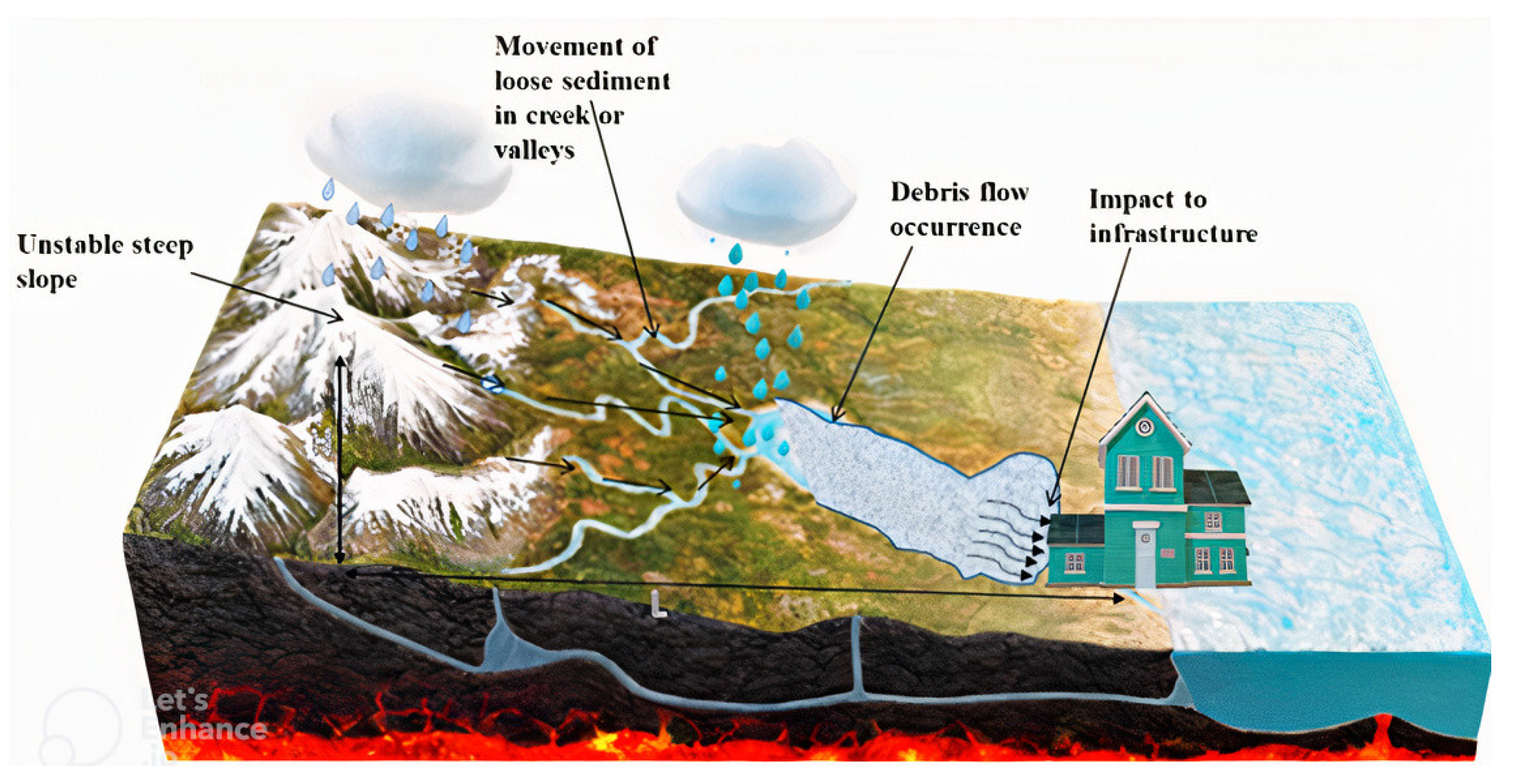
2. Debris Flow and Its Consequences

Debris flows are very rapid to extremely rapid non-plastic flows. It may be defined as the mixture of loose sediments and water that moves down in a steep channel [10,21]. A debris flow event may occur in a series of surges that travels several hundred kilometers with a velocity ranged 4–16 m/s [29]. Based on the moment transfer mechanism, many events are identified as debris slides, mudflows, debris floods, debris torrents, mud spates, and lahars [10,30,31]. However, this article only focuses on the debris flow and its consequences on the built environment. The debris flow density ranges from 1800 to 2400 kg/m³, twice the density of mud slurry [32,33]. Climate change (e.g., intense rainfall), deforestation, and earthquakes are the primary causes of debris flows [34,35,36].

Additionally, wildfires, melting glaciers, and disruption of snow cover distribution due to unfavorable weather conditions are other important factors triggering most debris flows in mountainous regions [37]. For instance, extensive rainfall for a long period initiates steep slope failure leading to massive sediment entertainment in the stream. These sediment movements later converted into disruptive events for many systems of infrastructure, as illustrated in Figure 1. The slope failure mechanism is a complex phenomenon caused by the reduction of cohesive forces between soil particles and the dissipation of pore pressure due to the infiltration of rainwater into the slope. Furthermore, additional load and relief, improperly designed or poorly executed drainage systems significantly affect the overall stability of slope [37,38].

Debris flow consequences are broadly divided into physical and socioeconomic impacts on customers or users of the infrastructure. Physical impacts are the most immediate ones, including injuries, fatalities, and emotional loss to victims, as well as complete to partial damage to infrastructures such as buildings, rail tracks, roads, and utility lines. On the other hand, the socioeconomic impact is the long-term impact due to the relocation of residences and loss of jobs and capital due to debris flow hazards.

According to the United States National Research Council (2011) [39], landslides caused an almost USD 1 billion loss in America, Japan, Italy, India, China, and the Soviet Union from 1960 to 1980. In addition, debris flow has damaged 390 commercial and residential buildings in China [40], 20 roads in South Korea [41], and several bridge piers in Romania [42]. Moreover, a debris flow event (1993) in the Kulekhani watershed, located in the lesser Himalayan region of Nepal, damaged the Amaluza dam. This dam was a component of the Paute hydroelectric plant, which supplied 65% of the electricity need consumed by Ecuador. Debris flood caused by dam failure severely damaged the hundreds of private homes and industrial complexes in the Rio Paute valley [43]. Therefore, estimation of the probability of debris flow occurrence and their extent with the vulnerability of elements at risk always support decision-makers in developing efficient mitigation and protection solutions. In this regard, researchers have been trying to develop different computational and analytical methods to estimate the possibility of hazard occurrence, loss to the built environment, and designing suitable risk reduction strategies for the last 20 years. Figure 2 represents the extensive research carried out in the vulnerability assessment of debris flow hazards by considering hazard intensity and damage by advanced monitoring technique, digital elevation model (DEM), and photogrammetry [31] from the United States to other subcontinents of the world. Figure 2 has been extracted by several sets of bibliographic analysis in VOS viewer software.

Furthermore, countries such as the United States, United Kingdom, Canada, China, and India continuously contribute to developing the landslide inventory, pre- and post-event data acquisition systems, and hybrid vulnerability assessment techniques for better risk management strategies.

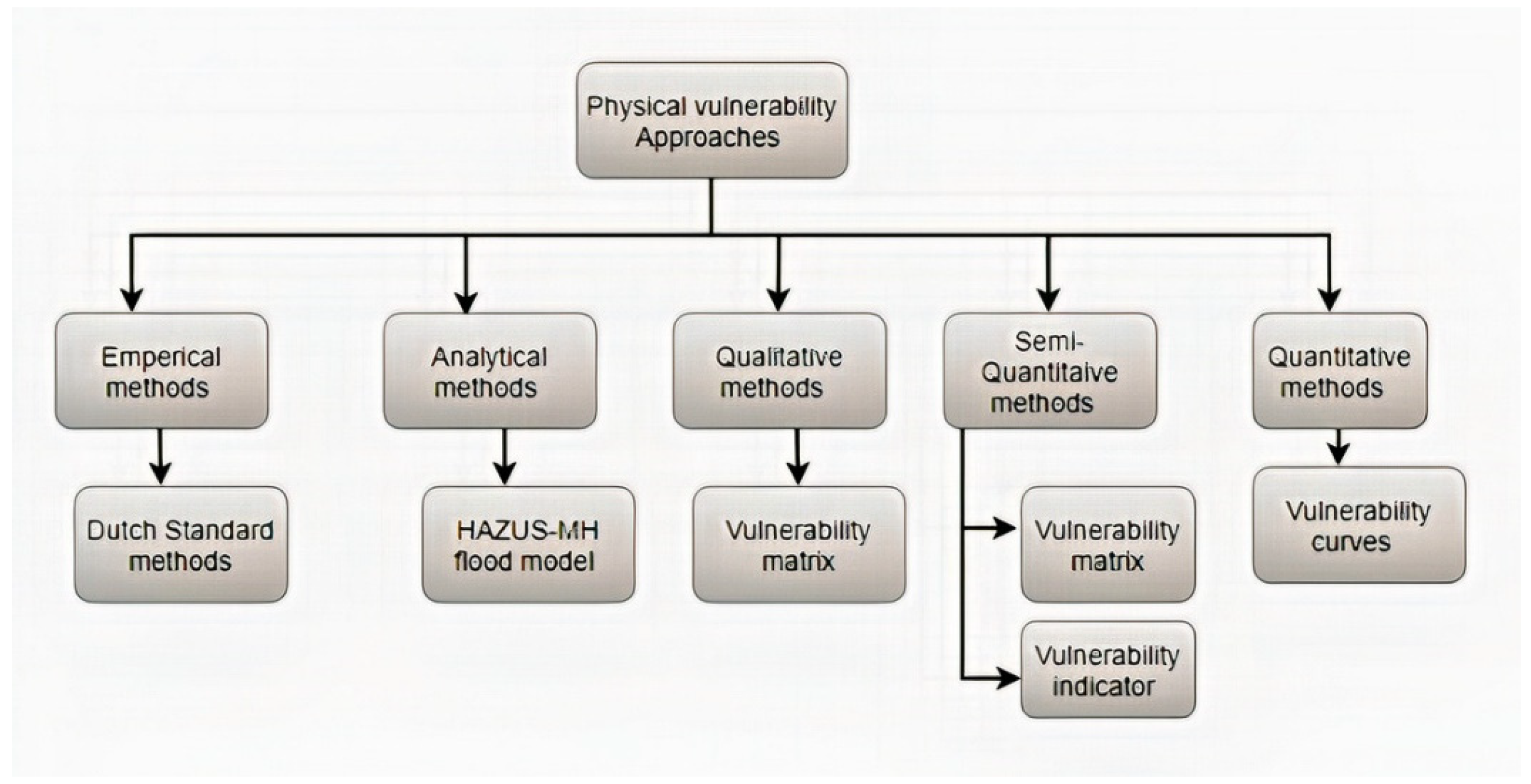
3. Overview of Physical Vulnerability Approaches

Various methodologies and techniques regarding physical vulnerability have been highlighted and demonstrated in the literature [44,45,46]. For example, empirical, analytical, qualitative, and quantitative methods, as shown in Figure 3, have been proposed to estimate the vulnerability of infrastructure subjected to mountainous hazards in the last two decades. Among these, vulnerability matrices (qualitative) [24,47,48], vulnerability curves (quantitative) [49,50], vulnerability indicators (semi-quantitative) [51,52,53], and integration of the different approaches [27,54] have been extensively used to assess the physical vulnerability of infrastructure.

Many physical vulnerability approaches have been developed for floods, earthquakes, and landslides. Therefore, this section highlights the vulnerability approaches, data requirements, benefits, and limitations developed for debris flows and floods impacting infrastructure (especially buildings). The vulnerability approaches and their application are summarized in Table 1. Table 1 is divided into vulnerability matrix, indicators, curves, and combined approaches for infrastructures (mainly buildings) affected by debris flows. Furthermore, process intensity such as deposition height (m), impact pressure (kPa), velocity (m/s), and their critical range have been highlighted and compared as responsible for complete to partial damage to the structure. Additionally, the degree of loss has been quantified from 0 to 1 quantitatively and qualitatively classified as minimal, moderate, heavy, and complete.

3.1. Empirical Methods

The empirical methods are based on the damage data from a historical event or expert opinion. It is expressed as vulnerability function and curves for a particular type of structure using damage surveys after the event. The damage is assessed using photogrammetry techniques by processing high-resolution satellite images and remote sensing data. The Dutch standard method (2004), as shown in Figure 4, is a good example of an empirical method that explains the eleven-depth damage function derived from damage data assessment and expert judgment [55]. Empirical methods are quick to calculate the vulnerability of structure in terms of equations and function but highly sensitive to the accuracy of the data, survey method, sample size, and detail of information [56]. Furthermore, methods are developed for mesoscale and use aggregate land-use data, affecting the quality of the vulnerability function.

The minimum level of information required to develop the empirical database has been illustrated in Figure 4 in the expert supervision of the hazard [56]. Overall, with an accurate dataset, empirical methods are suitable for developing the vulnerability function for a building of the same type and size, particularly for floods and earthquakes. The result is either a damage probability matrix (DPM) or vulnerability curves. However, the transferability of curves and functions is the main limitation of this method to other sites and structures.

3.2. Analytical Methods

Analytical methods investigate the behavior of infrastructure based on engineering design criteria, load, and forces responsible for the failure using physical modelling tests, (e.g., shake tables or wind tunnels) and computational techniques [57]. For instance, in the flooding vulnerability analysis of buildings, it is essential to possess different flood parameters, e.g., duration, velocity, and impact pressure [57]. Hazus_MH flood model [58] is a good example of an analytical approach for vulnerability assessment of a building subjected to flood. Furthermore, it can estimate the debris generated by building in tonnes/sqft. However, the model does not consider debris generated by vegetation and flood water.

Furthermore, it requires a large dataset to validate the model, and its transferability is the main limitation to other sites and structures. Empirical and analytical methods developed so far are mostly used for vulnerability assessment of floods. These approaches are used as complementary methods for vulnerability assessment of structures impacted by debris flows. Hence, this article is limited to discussing the vulnerability of structures subjected to debris flow hazard in detail based on Table 1, as shown below. In general, debris flow intensity and degree of loss are the primary variables for developing the vulnerability assessment framework. From Table 1, It can be observed that most of the researchers used debris height (h) ranged 0 to 6 m to develop vulnerability approach as flow depth data is easily available in post-event surveys. Further, debris flow velocity (v) and impact pressure (p) are also used to understand and categorize the damage class in various vulnerability approaches. The detail of each vulnerability approach with case studies has been discussed in a subsequent section.

Table 1. Review of existing vulnerability approach for mountainous hazard.

S. No.	Reference	Event/Location/Number of Structures Affected	Process Intensity	Damage Value/Classification	Remark
1	Zanchetta et al., 2004 [59]	6 May 1998/Italy/25 buildings	$v \ge 5 m{s}^{-1}$$,p\ge$ 35 kPa, l = 900–2000 m	Reconstruction value (€)/complete, heavy, and moderate	Vulnerability Matrix
2	Hu et al., 2012 [60]	7 August 2010/China/16 buildings	p = 0–110 kPa, Q = 1485 $m^3{s}^{-1}$, volume = 2.2 million $m^3$	Municipality value/complete (18 < p < 110 kPa), heavy, (8 < p < 50 kPa), moderate, (6 < p < 35 kPa), slight, (p ≤ 8 kPa), and very slight)	Vulnerability matrix
3	Jakob et al., 2012 [61]	68 well-documented date/20 buildings	$I_{DF}=d{v}^2$ $4 \le 31,500$ for slight damage to destruction	Insurance value/some sedimentation (I) < 25% of an insured loss, some structural damage (II) = 25–50% insured loss, major structural damage (III) > 75% insured loss, destruction (IV) = 100% loss	Vulnerability matrix
4	Winter et al., 2013 [62]	17 countries’ data/20 roads	volume = 10–10,000 m3	Limited, serious, and destroyed	Vulnerability matrix with fragility curve
5	Kang and Kim 2016 [63]	August 2011/South Korea/25 buildings	v = 3–14.9 m/s, d = 0–6 m, p = 0–35 kPa Q = 15.6–759.3 $m^3{s}^{-1}$	Property value/complete damage For non-RC building (p > 30 kPa) For RC building (p > 35 kPa)/NA	Vulnerability Curve For RC building $\mathrm{V}=1-e^{\left(-0.0094\ast v^{2.775}\right)}$, $\mathrm{V}=1-e^{\left(-0.17034\ast d^{1.537}\right)}$, $\mathrm{V}=1-e^{\left(-0.0005\ast p^{1.690}\right)}$
6	Fuchs et al. 2007 [55]	16 August 1997/Austria/16 buildings	h = 0–3 m	Reconstruction value (1600–140,000€)/NA	Vulnerability curves V = 0.11 h2–0.02 h, for h < 2.5 m and r2 = 0.865
7	Haugen and Kaynia 2008 [64]	6 May 1998/Italy/6 buildings	x = 0.015–0.127 m p = 0.1–1.15 MN	Insurance value/complete (0.45 < p <1.15 MN), extensive (0.34 < p < 0.81 MN), moderate (0.15 < p < 0.40), and slight (0.1 < p < 0.15)	Vulnerability model
8	Akbas et al., 2009 [49]	13 July 2008/Italy/20 buildings	h = 0.30–3 m	reconstruction value (€ 2000 to € 290,000)/damage factor (0–1)	Vulnerability curves V = 0.17 h2–0.03 h, r2 = 0.995
9	Papathoma-Köhle et al., 2012 [52]	August 1987/Italy/51 buildings	h = 0–4 m	Degree of loss based on photographic documentation and repair cost from the municipality (approx. 8.5 million €)/NA	Physical vulnerability curve $\mathrm{V}=1-e^{\left(-0.27{\left(\frac{h+1.287}{1.287}-1\right)}^{2.974}\right)}$
10	Quan Luna et al., 2011, 2014 [65,66]	13 July 2008/Italy/30 buildings	h = 0–4 m $\mu =0–6$ m2s p = 0–40 kPa	Reconstruction value (€)/damage index (0.35 to 0.66)	Vulnerability curve $\mathrm{V}=\frac{1.49\ast {\left(\frac{h}{2.513}\right)}^{-1.938}}{{\left(1+\frac{h}{2.513}\right)}^{-1.938}}$$\mathrm{for} \mathrm{h} \le$$3.63 \mathrm{m}$ $\mathrm{V}=1 \mathrm{for} \mathrm{h} \ge$$3.63 \mathrm{m}$ $\mathrm{V}=\frac{5.28\ast {\left(\frac{\mu }{29.26}\right)}^{-0.867}}{{\left(1+\frac{\mu }{29.26}\right)}^{-0.867}}$$\mathrm{for} \mu \le$$5.32 {\mathrm{m}}^2\mathrm{s}$ $\mathrm{V}=1 \mathrm{for} \mu \ge$ 5.32 m2s
11	Totschnig and Fuchs 2013 [28]	16 August 2005/Austria/193 buildings	h = 0–4 m IR = 0–0.60	Property value (€)/damage ratio (0–1)	Vulnerability model $\mathrm{V}=1-e^{-1.253{\left(\frac{I+2.438}{2.438}-1\right)}^{1.892}}$$(\mathrm{Weibull} \mathrm{method})$ $\mathrm{V}=\frac{1}{1+{\left(\frac{tan{I}_{R.}\pi /2+0.34}{0.342}-1\right)}^{-2.492}}$ (Log logistic)
12	Ciurean et al., 2017 [67]	1998/Italy/41 building (1–3 floors)	Iobs = 0.1 hdpt	Municipality value (€)/damage ratio DR = DC/MV = 0.15–0.90	Vulnerability model $1.V=\left\{\begin{array}{c}0, I<a \\ \frac{{\left(I-a\right)}^2}{\left(b-a\right)\left(c-a\right)}, a\le I\le c\\ 1-\frac{{\left(b-I\right)}^2}{\left(b-a\right)\left(c-a\right)}, c<I\le b \\ 1 I>b\end{array}\right\}$$, \mathrm{DR}=\frac{{\left(I-a\right)}^2}{\left(b-a\right)\left(c-a\right)}$ $2.V=\left\{\begin{array}{c} 2\frac{{\left(I\right)}^2}{{\left(R\right)}^2}, \frac{I}{R}\le 0.5\\ 1-\frac{2{\left(R-I\right)}^2}{{\left(R\right)}^2}, 0.5<\frac{I}{R}\le 1.0 \\ 1 \frac{I}{R}>1.0\end{array}\right\}$
13	Shen et al., 2018 [68]	14 August 2010/China 390 buildings	h = 0–3.5 m $v=1–7$ m/s p = 0–35 kPa	Reconstruction value (€)/degree of loss (0.25–0.85)	Vulnerability curve
14	Yan et al., 2020 [69]	September 2010/China/2 bridge pier	v = 1–12 m/s h = 0–6 m Rb = 0.1–0.80 m	Insurance value (€)/4 damage classes (0.2–1)	Physical vulnerability curve (Damage class 3) $\mathrm{V}=0.997-\frac{1.025 }{{\left(1+\frac{h}{3.514}\right)}^{3.838}}$ $\mathrm{V}=0.979-\frac{1.031}{{\left(1+\frac{v}{3.47}\right)}^{3.193}}$ $\mathrm{V}=0.858-\frac{0.867}{{\left(1+\frac{R_b}{0.275}\right)}^{11.86}}$
15	Kappes et al., 2012 [70]	Well-documented debris flow data/65 buildings	Building surrounding, building, and human-related characteristics,	N/A	Indicator based vulnerability
16	Godfrey et al., 2015 [54]	2004,2005/Romania/60 buildings	h = 0–3 m d = 0–5 m	Municipality report (€)/damage factor (0-1)	Specific vulnerability curve
17	Du et al., 2015 [15]	19 September 1982/El Salvador/58 buildings	p = 4.5–14 kPa	Susceptibility factor Sstr = 0.1–0.8 for reinforced-to-brick masonry structure	Vulnerability model $\mathrm{V}=\left\{\begin{array}{c}\frac{1}{2}{\left(\frac{I}{1-S}\right)}^2 I\le 1-S\\ 1-\frac{1}{2}{\left(\frac{1-I}{S}\right)}^2 I>1-S\end{array}\right\}$
18	Dadfar et al., 2018 [71]	Arbitrary data/pipeline	D/t = 36, 64, 78, and 96. PGD width = 10, 20, 30 m	NA/Tensile rupture, local buckling, and premature cross-sectional failure	Novel vulnerability function repair rate = P.(E) * vALD* (repair rate) ALD
19	Wu and Li, 2019 and Mustaffa et al., 2021 [29,72]	Debris flow data from China, Malaysia/pipeline	Exposed width = 10–40 m $\theta$ = 15°–90° width of the corrosion pit = 0.3–2 m. p = 42.6 to 600 kPa	Shear failure observed due to impact of stone/NA	A multivariate regression equation for corrosion parameters of the pipeline $=187.138\ast \frac{t}{T}+149.618\ast \frac{b}{\pi D}+22.276\ast \frac{l}{\sqrt{50DT}}+410.03$
20	Thouret et al., [53]	2004/Venezuela/15 buildings	Building type, Number of floors, age of construction	Reconstruction value (€)/damage was assessed using 3 × 3 DEM file of the study area	Physical vulnerability maps for city block, and residential building

Note: The abbreviation and symbol used in Table 1 have been described at the end of the manuscript.

Table 1. Review of existing vulnerability approach for mountainous hazard.

S. No.	Reference	Event/Location/Number of Structures Affected	Process Intensity	Damage Value/Classification	Remark
1	Zanchetta et al., 2004 [59]	6 May 1998/Italy/25 buildings	$v \ge 5 m{s}^{-1}$$,p\ge$ 35 kPa, l = 900–2000 m	Reconstruction value (€)/complete, heavy, and moderate	Vulnerability Matrix
2	Hu et al., 2012 [60]	7 August 2010/China/16 buildings	p = 0–110 kPa, Q = 1485 $m^3{s}^{-1}$, volume = 2.2 million $m^3$	Municipality value/complete (18 < p < 110 kPa), heavy, (8 < p < 50 kPa), moderate, (6 < p < 35 kPa), slight, (p ≤ 8 kPa), and very slight)	Vulnerability matrix
3	Jakob et al., 2012 [61]	68 well-documented date/20 buildings	$I_{DF}=d{v}^2$ $4 \le 31,500$ for slight damage to destruction	Insurance value/some sedimentation (I) < 25% of an insured loss, some structural damage (II) = 25–50% insured loss, major structural damage (III) > 75% insured loss, destruction (IV) = 100% loss	Vulnerability matrix
4	Winter et al., 2013 [62]	17 countries’ data/20 roads	volume = 10–10,000 m3	Limited, serious, and destroyed	Vulnerability matrix with fragility curve
5	Kang and Kim 2016 [63]	August 2011/South Korea/25 buildings	v = 3–14.9 m/s, d = 0–6 m, p = 0–35 kPa Q = 15.6–759.3 $m^3{s}^{-1}$	Property value/complete damage For non-RC building (p > 30 kPa) For RC building (p > 35 kPa)/NA	Vulnerability Curve For RC building $\mathrm{V}=1-e^{\left(-0.0094\ast v^{2.775}\right)}$, $\mathrm{V}=1-e^{\left(-0.17034\ast d^{1.537}\right)}$, $\mathrm{V}=1-e^{\left(-0.0005\ast p^{1.690}\right)}$
6	Fuchs et al. 2007 [55]	16 August 1997/Austria/16 buildings	h = 0–3 m	Reconstruction value (1600–140,000€)/NA	Vulnerability curves V = 0.11 h2–0.02 h, for h < 2.5 m and r2 = 0.865
7	Haugen and Kaynia 2008 [64]	6 May 1998/Italy/6 buildings	x = 0.015–0.127 m p = 0.1–1.15 MN	Insurance value/complete (0.45 < p <1.15 MN), extensive (0.34 < p < 0.81 MN), moderate (0.15 < p < 0.40), and slight (0.1 < p < 0.15)	Vulnerability model
8	Akbas et al., 2009 [49]	13 July 2008/Italy/20 buildings	h = 0.30–3 m	reconstruction value (€ 2000 to € 290,000)/damage factor (0–1)	Vulnerability curves V = 0.17 h2–0.03 h, r2 = 0.995
9	Papathoma-Köhle et al., 2012 [52]	August 1987/Italy/51 buildings	h = 0–4 m	Degree of loss based on photographic documentation and repair cost from the municipality (approx. 8.5 million €)/NA	Physical vulnerability curve $\mathrm{V}=1-e^{\left(-0.27{\left(\frac{h+1.287}{1.287}-1\right)}^{2.974}\right)}$
10	Quan Luna et al., 2011, 2014 [65,66]	13 July 2008/Italy/30 buildings	h = 0–4 m $\mu =0–6$ m2s p = 0–40 kPa	Reconstruction value (€)/damage index (0.35 to 0.66)	Vulnerability curve $\mathrm{V}=\frac{1.49\ast {\left(\frac{h}{2.513}\right)}^{-1.938}}{{\left(1+\frac{h}{2.513}\right)}^{-1.938}}$$\mathrm{for} \mathrm{h} \le$$3.63 \mathrm{m}$ $\mathrm{V}=1 \mathrm{for} \mathrm{h} \ge$$3.63 \mathrm{m}$ $\mathrm{V}=\frac{5.28\ast {\left(\frac{\mu }{29.26}\right)}^{-0.867}}{{\left(1+\frac{\mu }{29.26}\right)}^{-0.867}}$$\mathrm{for} \mu \le$$5.32 {\mathrm{m}}^2\mathrm{s}$ $\mathrm{V}=1 \mathrm{for} \mu \ge$ 5.32 m2s
11	Totschnig and Fuchs 2013 [28]	16 August 2005/Austria/193 buildings	h = 0–4 m IR = 0–0.60	Property value (€)/damage ratio (0–1)	Vulnerability model $\mathrm{V}=1-e^{-1.253{\left(\frac{I+2.438}{2.438}-1\right)}^{1.892}}$$(\mathrm{Weibull} \mathrm{method})$ $\mathrm{V}=\frac{1}{1+{\left(\frac{tan{I}_{R.}\pi /2+0.34}{0.342}-1\right)}^{-2.492}}$ (Log logistic)
12	Ciurean et al., 2017 [67]	1998/Italy/41 building (1–3 floors)	Iobs = 0.1 hdpt	Municipality value (€)/damage ratio DR = DC/MV = 0.15–0.90	Vulnerability model $1.V=\left\{\begin{array}{c}0, I<a \\ \frac{{\left(I-a\right)}^2}{\left(b-a\right)\left(c-a\right)}, a\le I\le c\\ 1-\frac{{\left(b-I\right)}^2}{\left(b-a\right)\left(c-a\right)}, c<I\le b \\ 1 I>b\end{array}\right\}$$, \mathrm{DR}=\frac{{\left(I-a\right)}^2}{\left(b-a\right)\left(c-a\right)}$ $2.V=\left\{\begin{array}{c} 2\frac{{\left(I\right)}^2}{{\left(R\right)}^2}, \frac{I}{R}\le 0.5\\ 1-\frac{2{\left(R-I\right)}^2}{{\left(R\right)}^2}, 0.5<\frac{I}{R}\le 1.0 \\ 1 \frac{I}{R}>1.0\end{array}\right\}$
13	Shen et al., 2018 [68]	14 August 2010/China 390 buildings	h = 0–3.5 m $v=1–7$ m/s p = 0–35 kPa	Reconstruction value (€)/degree of loss (0.25–0.85)	Vulnerability curve
14	Yan et al., 2020 [69]	September 2010/China/2 bridge pier	v = 1–12 m/s h = 0–6 m Rb = 0.1–0.80 m	Insurance value (€)/4 damage classes (0.2–1)	Physical vulnerability curve (Damage class 3) $\mathrm{V}=0.997-\frac{1.025 }{{\left(1+\frac{h}{3.514}\right)}^{3.838}}$ $\mathrm{V}=0.979-\frac{1.031}{{\left(1+\frac{v}{3.47}\right)}^{3.193}}$ $\mathrm{V}=0.858-\frac{0.867}{{\left(1+\frac{R_b}{0.275}\right)}^{11.86}}$
15	Kappes et al., 2012 [70]	Well-documented debris flow data/65 buildings	Building surrounding, building, and human-related characteristics,	N/A	Indicator based vulnerability
16	Godfrey et al., 2015 [54]	2004,2005/Romania/60 buildings	h = 0–3 m d = 0–5 m	Municipality report (€)/damage factor (0-1)	Specific vulnerability curve
17	Du et al., 2015 [15]	19 September 1982/El Salvador/58 buildings	p = 4.5–14 kPa	Susceptibility factor Sstr = 0.1–0.8 for reinforced-to-brick masonry structure	Vulnerability model $\mathrm{V}=\left\{\begin{array}{c}\frac{1}{2}{\left(\frac{I}{1-S}\right)}^2 I\le 1-S\\ 1-\frac{1}{2}{\left(\frac{1-I}{S}\right)}^2 I>1-S\end{array}\right\}$
18	Dadfar et al., 2018 [71]	Arbitrary data/pipeline	D/t = 36, 64, 78, and 96. PGD width = 10, 20, 30 m	NA/Tensile rupture, local buckling, and premature cross-sectional failure	Novel vulnerability function repair rate = P.(E) * vALD* (repair rate) ALD
19	Wu and Li, 2019 and Mustaffa et al., 2021 [29,72]	Debris flow data from China, Malaysia/pipeline	Exposed width = 10–40 m $\theta$ = 15°–90° width of the corrosion pit = 0.3–2 m. p = 42.6 to 600 kPa	Shear failure observed due to impact of stone/NA	A multivariate regression equation for corrosion parameters of the pipeline $=187.138\ast \frac{t}{T}+149.618\ast \frac{b}{\pi D}+22.276\ast \frac{l}{\sqrt{50DT}}+410.03$
20	Thouret et al., [53]	2004/Venezuela/15 buildings	Building type, Number of floors, age of construction	Reconstruction value (€)/damage was assessed using 3 × 3 DEM file of the study area	Physical vulnerability maps for city block, and residential building

Note: The abbreviation and symbol used in Table 1 have been described at the end of the manuscript.

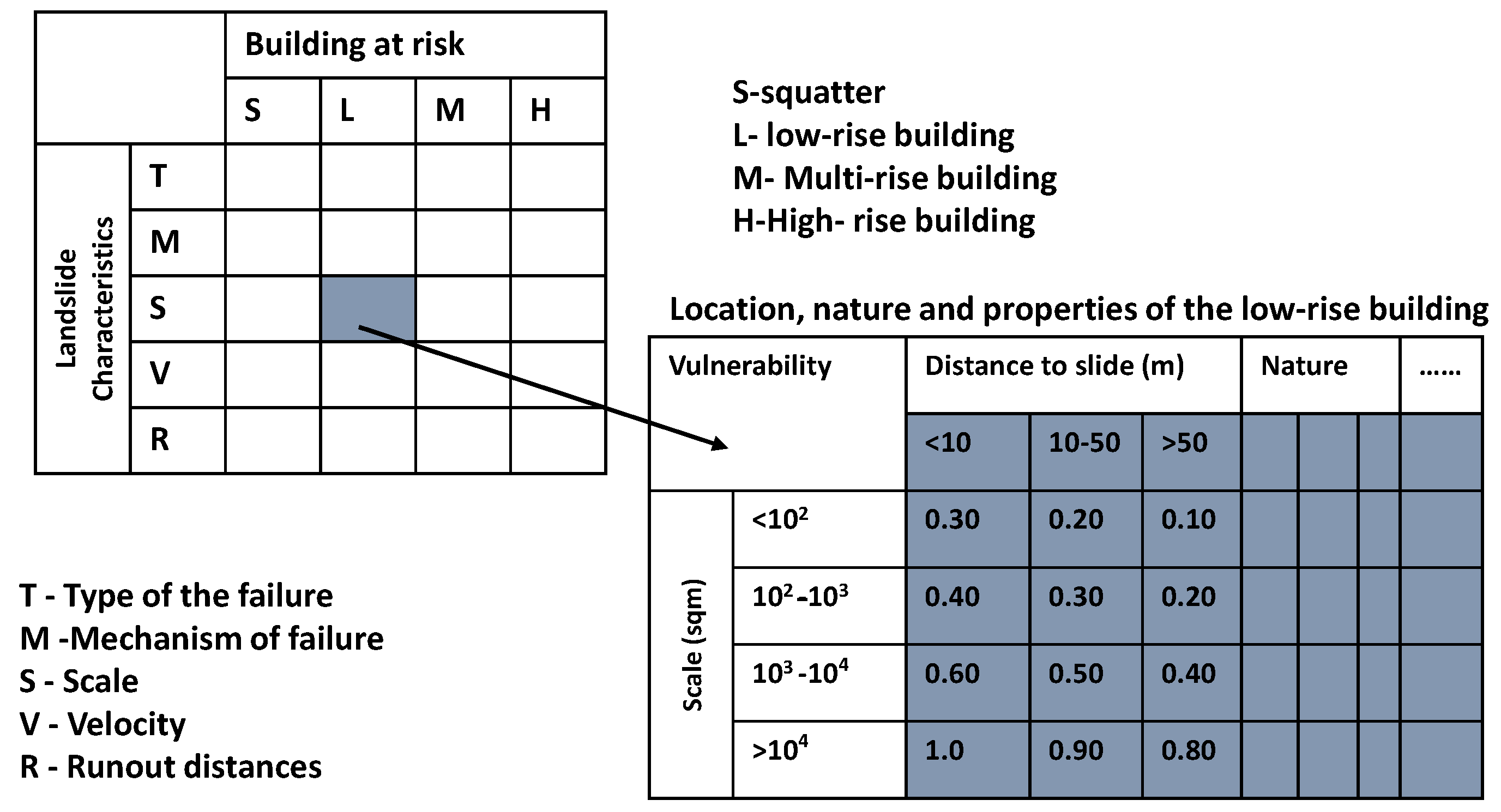
3.3. Qualitative Methods (Vulnerability Matrix)

The vulnerability matrix is a qualitative method to assess the vulnerability of infrastructure subjected to torrential hazards. The method is always supported by a detailed vulnerability assessment approach, such as empirical and expert judgment [73]. The debris flow intensity is expressed as impact pressure, viscosity, debris height, or velocity ranges. The damage level has been described as slight, moderate, significant, partial, complete, and heavily damage based on post-event surveys and expert judgment [62,63,74]. In the present paper, six vulnerability matrix studies are reviewed (see Table 1), and their applicability is discussed in detail. Initially, Leon et al., 1996 [73] attempted to present landslides’ vulnerability matrices discussing various damage levels as slight to complete, corresponding to the depositional height from 0.30 to 3 m resulting in a vulnerability value (from 0 to 1). Similarly, Zanchetta et al., 2004 [59] presented detailed matrices using impact pressure, velocity, and runout distances for volcanoclastic debris flow in the same region. It was more robust and significant compared to Leone et al., 1997 [74] matrices as it relates the intensity to damage more appropriately.

Moreover, Jakob et al., 2012 [61] analyzed the data of 66 well-documented debris flow case studies to present a unique damage probability matrix based on avg. Impact index (I_DF) and four damage classes as mentioned in Table 1. This matrix utilized flow depth and velocity, making it more reliable than other vulnerability matrices. Therefore, it can be stated that vulnerability matrices can make the relationship between process and consequences clear and easy to understand by a non-expert. Additionally, vulnerability matrices are flexible to a certain degree and reduce subjectivity compared with vulnerability curves. However, this method’s transferability and comparison possibilities are limited to the structure’s region and characteristics. Furthermore, this method does not provide information regarding the financial value or monetary loss [27]. For instance, Figure 5 represents the vulnerability matrix for low to high-rise buildings based on landslide characteristics length (m) and building properties that classify the stepwise damage levels [73].

Overall, the vulnerability matrix provides the correlation between rate of loss to the exposed elements and load generated by debris flow phenomena. Further, they offer a coherent framework of structural vulnerability by considering nature, characteristics of hazards, and buildings.

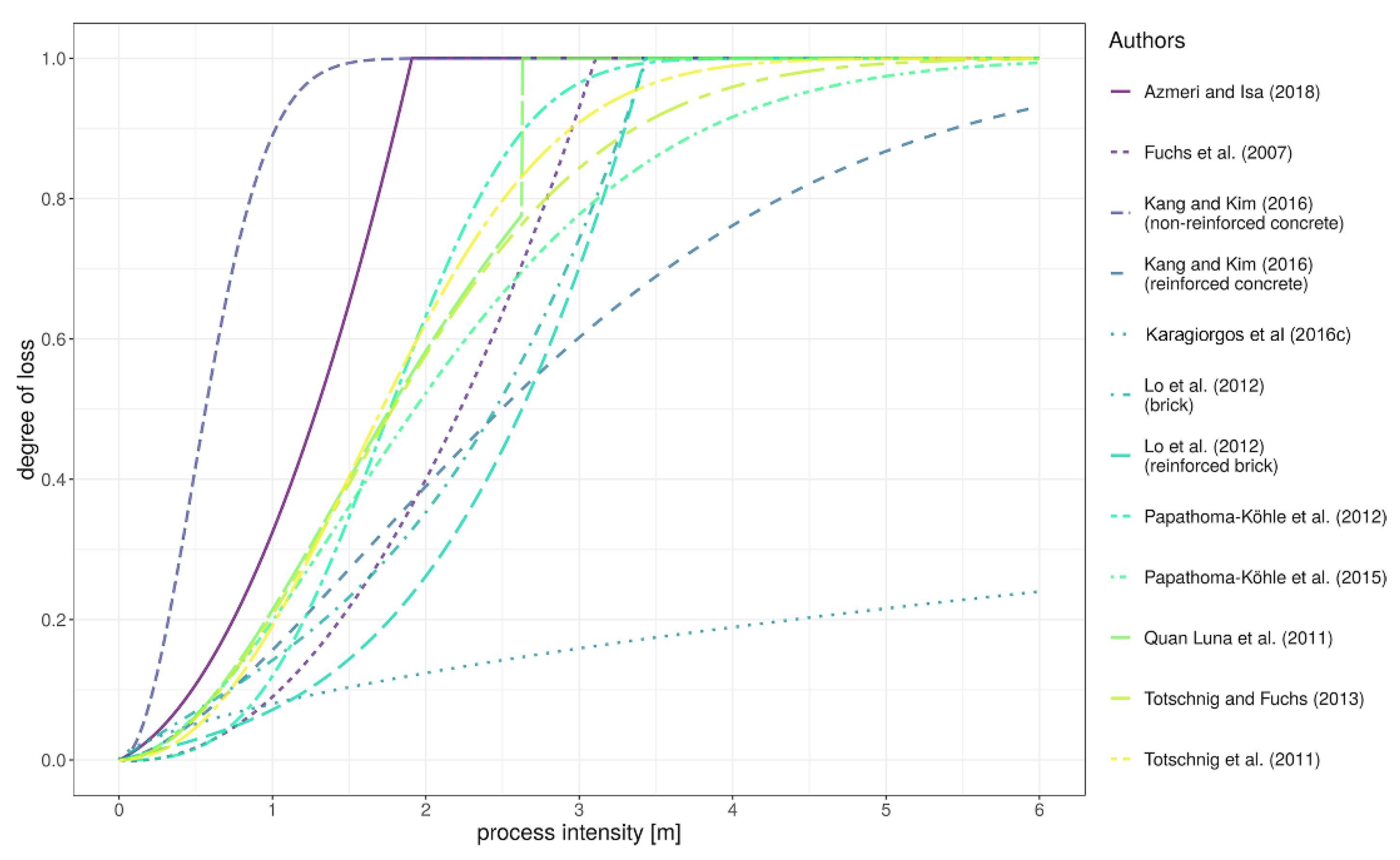
3.4. Quantitative Method (Vulnerability Curve)

Vulnerability curves (or functions) are quantitative methods that mainly focus on the degree of loss rather than the probability of occurrence (in the fragility curve). Hence, a large amount of reliable empirical data is required. Process intensity may be debris flow height, velocity, impact pressure, and viscosity, which can produce different vulnerability curves for the same degree of loss. The intensity of debris flow is obtained by field surveys [8,75], experimental methods [22,40,76], and numerical techniques [77,78,79,80,81]. On the other hand, damage estimation can be done by direct (insurance companies) and indirect methods, photographic documentation, and earth observation data [74,82]. Afterward, the degree of loss is evaluated from the property’s damage cost and value, which then integrated with process intensity in the form of a function or vulnerability curve. Different vulnerability functions were developed by researchers [63,65,83] and compared in Figure 6 using the process intensity as flow depth (m) and degree of loss.

Apart from the curve produced by Karagiorgos et al., 2016 [84], it is clear that all other curves exhibit a steady rise in the degree of loss between 1 m and 3 m process intensity. Differences in the curve may be due to the material used in case studies, building architecture, and the consideration of process intensity. Further, statistical analysis of available data also differs in the vulnerability function and shape of the curve. Therefore, a direct comparison of different vulnerability curves is quite challenging because significant variation in process intensity and approaches of researchers was observed among the studies [85]. Totsching and Fuchs, 2013 [28] presented the vulnerability curve based on damage data of Austria by introducing relative intensity, which can incorporate the buildings of different heights in the same curve. Furthermore, Papathoma-Köhle et al., 2016 [52] attempted to improve the existing vulnerability curve in South Tyrol by considering the building type, detailed monetary loss based on repair rate and suggested the specific vulnerability function as mentioned in Table 1 and Figure 6 for a future event. Additionally, interpolation of the intensity (especially velocity and impact pressure) for an individual building may significantly increase uncertainties [38].

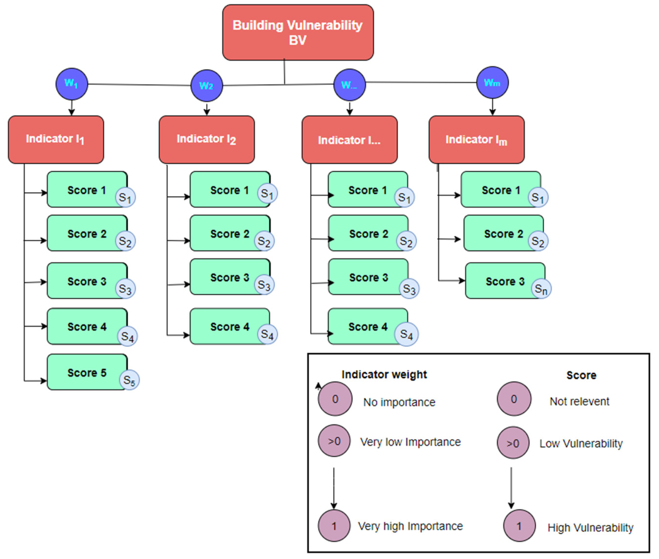
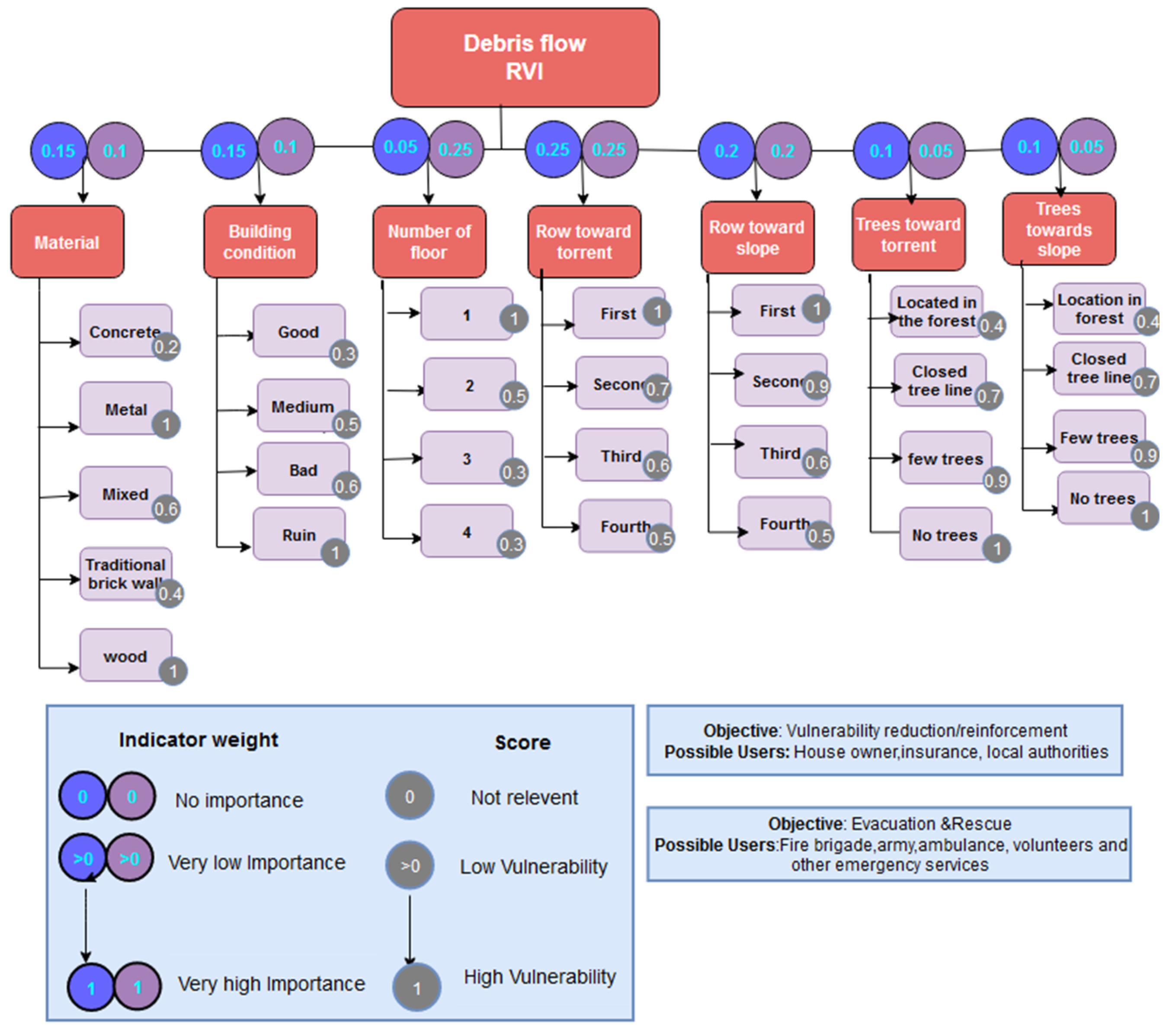
3.5. Semi-Quantitative Methods (Vulnerability Indicator)

Birkmann [51] first stressed the social vulnerability that described the vulnerability indicator as a variable to incorporate the building characteristics and the structure’s orientation. It was an operational representation of the structure’s characteristics and quality, focusing on its coping capacity, resilience characteristics, impact, and susceptibility of the system to natural hazards [86]. It enables the decision-maker to analyze the disaster’s effect on the population’s social, economic, and environmental conditions. This approach incorporates the relevant indicator selection, variable identification, weighting, and integration into the vulnerability index. In this context, Kappes et al., 2012 [70] did remarkable work in developing a vulnerability indicator approach by explaining the parameter process, scoring, and weighting techniques, as shown in Figure 7 and Figure 8. However, the parameter’s weighing varies with the type of study, the importance of the structural element, exposure of the element, or expert judgment. Three major groups of vulnerability indicators are suggested for examining buildings in mountainous regions vulnerable to debris flow hazards. Building-specific information such as material, number of floors, age, height, type of foundation and other characteristics are influenced more or less by debris flow hazard. Building surroundings provide protection from various hazards but are rarely taken into account. Spatial distribution and characteristic of the population in hazardous areas is always crucial information for emergency planners and civil protection strategies [70]. Once the relevant indicators have been collected, scoring and weighting are performed by considering the type of hazard, purpose of the study, and use of infrastructure.

For example, the first floor of the building is highly vulnerable to debris flow impact. Hence its score should always be greater than other floors. Similarly, from Figure 8, suppose most of the material used in the construction is wood or any weaker material than reinforced concrete (RCC); in that case, it is severely affected by the debris flow hazard and should score higher than concrete. Furthermore, researchers such as Thouret et al., 2014 [53] considered the building type, roof type, number and quality of openings, and the number of stories as an indicator to assess the physical vulnerability of a residential building in Peru. Similarly, Ettinger et al., 2015 [87] developed the relationship using a logistic regression technique between the indicator and damage to estimate the damage probability index. The leading indicators were the building footprint, shape of the city block, distances from the channel, building density, number of stories, and soil permeability to develop the efficient vulnerability approach.

Moreover, Papathoma-Köhle et al., 2019 [86] improved the criteria of indicators selection based on relevancy and presented the new physical vulnerability index (PVI), which was later used in Europe and other sites where no empirical data are available for vulnerability assessment. Each indicator-based methodology contained a list of indicators relevant to the physical vulnerability assessment of the structure (building) for debris flow hazard. Some indicators used in these studies are common (e.g., building type), but it mostly depends on the expert judgment and the requirement of the study.

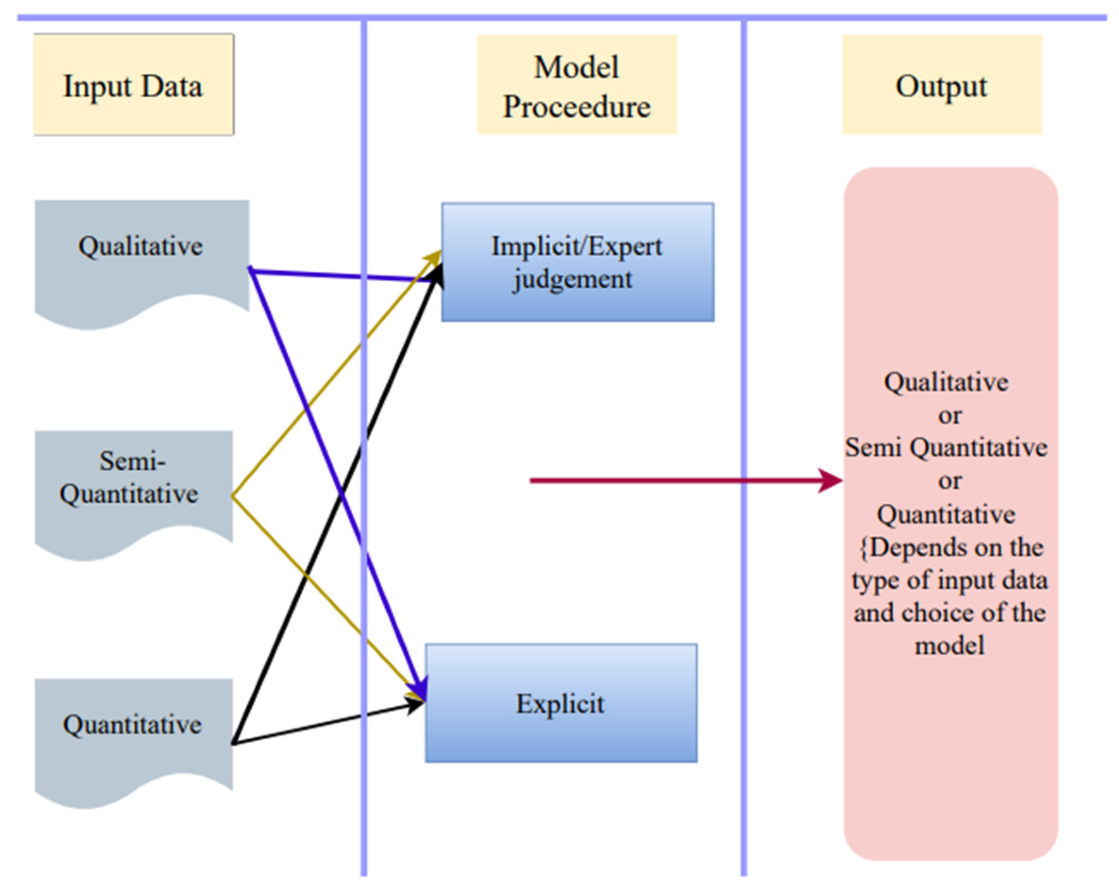
3.6. Combination of Approaches

Each method described above has limitations due to data scarcity, damage prediction, estimation of process intensities, and other miscellaneous factors. Hence, researchers attempted to combine the approaches to increase their robustness by reducing the uncertainties. Therefore, an indicator is used as a complementary approach to well-established methods (such as vulnerability curves) to add benefits of both methods. In this regard, Fuchs et al., 2019 [83] recently integrated vulnerability curves and indicators to quantify the physical vulnerability of residential buildings in Martell (Italy) and their interaction with the element at risk. They commented that the intensity of debris flow should also be considered as an essential indicator in the indicator-based methodology in expressing the physical resilience of the building. In this way, intensity can thus be viewed as a process characteristic that includes debris flow height and direction. This study provided the relative vulnerability index (RVI) expression based on the score, intensity, and weight of the parameter as represented by Equation (1)

$$\mathrm{RVI} ={⅀}_1^m{\mathrm{w}}_m{I}_m{\mathrm{s}}_n$$

(1)

where w = weights, I = indicators, s is the scores of the indicators.

Furthermore, Du et al., 2015 [15] presented a vulnerability model using susceptibility of debris flow hazard (S) and intensity (I) of flow described by Equation (2). The set of indicators selected were the structure characteristics, service year, level of maintenance, and structure orientation with respect to flow. This methodology was later applied to eight debris flow events in San Salvador (Italy).

$$\mathrm{V}=\left\{\begin{array}{c}\frac{1}{2}{\left(\frac{\mathrm{I}}{1-\mathrm{S}}\right)}^2 \mathrm{I}\le 1-\mathrm{S}\\ 1-\frac{1}{2}{\left(\frac{1-\mathrm{I}}{\mathrm{S}}\right)}^2 \mathrm{I}>1-\mathrm{S}\end{array}\right\}$$

(2)

where V ℇ [0, 1] is the vulnerability of the element at risk, I ℇ [0, 1] is the intensity of the landslide, S ℇ [0, 1] is the susceptibility. If V, I, S = 0 means less degree of damage, the landslide’s negligible damage potential and vulnerable element have high resistance to landslide impact, respectively. If V, I, S =1, the structure completely collapses, the intensity has an enormous damage potential, and the element is highly susceptible to landslide. Here, V, I, and S are non-dimensional terms. Similarly, Godfrey et al., 2015 [71] combined the generic vulnerability curve (GVC) with the vulnerability index (VI) based on a set of indicators to produce a specific vulnerability curve (SVC) Martell (Italy).

Recapitulating the above section vulnerability assessment is undoubtedly the prerequisite step of the risk reduction system. It is one of two counterparts of the risk assessment process. Most of the approaches discussed above differ not only by a basic principle, such as understanding and expression of vulnerability, but also in their detail, such as number and type of structure under investigation. Each vulnerability methodologies have some drawbacks and benefits summarized in

Table 2. Summary of the vulnerability approach.

Approaches	Advantages	Limitation
Vulnerability matrices	A qualitative method, post-event data are likely to be less required. The matrices formed are simple and easy to understand by a non-expert and end user.	The results obtained may not be transformed into a monetary loss. Assessment of damage is specific to process intensity and element at risk. The transferability of matrices to other sites and structures is limited.
Vulnerability curve	It is a quantitative method, and loss can be translated into monetary cost. A single vulnerability curve can incorporate different sizes of buildings. Curves may form the basis for assessing future scenario losses and costs.	Important information about the structure’s orientation and construction material is missing. Process intensity characteristics (e.g., direction of flow and duration) are ignored. It required large ex-post quality data, and highly site-specific Transferability and comparison are also challenging for a different type of infrastructure
Vulnerability indicator	Characteristics of elements at risk are considered. It is flexible and can be adjusted to account for different hazards and specific user needs.	Weighting and scoring of indicators required expert judgment. Most indicators considered the characteristic of structures rather than the process intensity of the hazard. Extensive field surveys are required since most of the information is not available at the local scale. At last result can not translate into the monetary cost.
Combined approach	Process intensity (flow depth, impact pressure, velocity) are considered with characteristics of element at risk. Specific vulnerability curve (SVC), and relative vulnerability index (RVI) is an example of an integrated approach that minimizes the uncertainty of matrices curves and indicators to some extent.	It is always quite difficult to score the indicator and their interaction with curves due to high-quality data requirements and expert opinion. Sometimes hybrid approach overestimates the losses due to uncertainties in damage assessment.

. They can be used based on required data availability, the study’s aim, and financial restrictions. Significant attempts have been made in the literature to quantify the intensity and damage associated with debris flow using interpolation techniques and satellite data. However, the scarcity of well-documented data, the limitation of each approach, and the debris flow assessment process stressed the researchers to develop more advanced tools to incorporate different aspects in the vulnerability assessment framework. Nevertheless, some well-documented debris flow events, such as Sarno and Martell (Italy), provided abundant data regarding intensity and damage to apply more than one vulnerability approach effectively. Further, hybrid vulnerability approaches by integrating different methodologies have gained popularity in the current scenario.

4. Uncertainties in Vulnerability Analysis

Uncertainties associated with debris flow susceptibility and vulnerability assessment often attract engineers to quantify it for accuracy in the risk management system. However, uncertainties, if not quantified and conserved, make the system inefficient and may overlook critical scenarios [28]. In addition, uncertainty might result in descriptive, aggregation, and judgmental errors in the vulnerability assessment systems. Therefore, uncertainties within the risk assessment process may be classified as aleatory and epistemic uncertainty. Aleatory uncertainties may be accidental due to variability of the physical properties, which cannot be reduced [85]. In comparison, epistemic uncertainty is due to a lack of or limited knowledge and can be reduced by a skilled workforce, increasing the number of tests, updating measurement methods, or improving computational procedures [88]. Uncertainty may also occur due to the characterization of exposure, input data, modeling methods, or output in vulnerability assessment systems. The potential uncertainties at various levels of vulnerability assessment methodologies are shown in Figure 9.

Input uncertainty may be caused by variable input data or a lack of expertise. Model/procedure uncertainty is a conceptual uncertainty that shows how the real world is represented and abstracted [28]. Finally, the uncertainty in the output is an aggregation of uncertainty associated with input parameters and model uncertainty [88]. Uncertainties associated with vulnerability curves are partly due to process intensity estimation, such as velocity, height, and impact pressure. Additionally, it may also occur due to monetary damage assessment methodologies, e.g., in some cases, the market value [89] of a building is used, whereas in other cases [28,53], reconstruction values are utilized.

Furthermore, the value of a building is determined by its size, which is a source of uncertainties in the vulnerability curve. A more detailed study of uncertainty related to the vulnerability curve was carried out by Eidsvig et al., 2014 [88] using uncertainty bands to communicate the uncertainties of the vulnerability curve to stakeholders to assist them in decision-making. Besides, some uncertainties regarding selecting the most relevant indicator, weighting approach, and aggregation of indicators, are also observed in indicator-based methodologies.

Uncertainty Quantification Techniques

Uncertainties in risk assessment systems can be handled by conservation or simply by ignoring them. But sometimes, later cases give highly unreliable results in a critical scenario of the vulnerability assessment system. On the other hand, conserving uncertainties may result in un-economic mitigation measures but mostly on the safe side [88,89]. Quantitative vulnerability assessment allows the estimation of landslide vulnerability uncertainties, such as employing confidence bands for the best-fitting function in vulnerability curves [90] and the first-order moment (FOSM) approach to assess the uncertainty in the input parameter [91]. Furthermore, the Monto–Carlo simulation is a trustworthy method for calculating the uncertainty in vulnerability systems of landslides initiated by rainfall [92]. It was developed as an experimental probabilistic method to solve difficult deterministic problems, since computers can easily simulate many trials with random results. Moreover, the model–structure-independent approach based on information theory proved effective in estimating epistemic and aleatory uncertainties during runoff modeling [93]. Information theory depends on the entropy principle, which characterizes the uncertainty of the chosen variable within the vulnerability model. Additionally, uncertainty associated with vulnerability curves was quantified by suggesting the best fit model by adjusting the error, which might be additive or multiplicative based on statistical analysis. The multiplicative uncertainty factor is commonly used in most geotechnical reliability analyses [85,94] to distribute the errors.

Moreover, numerous studies are available using Weibull distribution, whereas some other studies used second- or third-order logistic regression to examine the relationship between damage and process intensity, as highlighted in

Table 3. Uncertainty quantification techniques in quantitative vulnerability approach.

Reference	Quantification Techniques	Characteristics
Uzielii 2006 and 2008 [90,97]	First-order moment approach (FOSM)	Confidence band using expert opinion helps to estimate uncertainties at the input stage.
Uzielii 2009 [92], Papadopoulos, and Hoi Yeung 2001 [98]	Monto–Carlo simulation	The Monte Carlo method readily considers all non-linearities. Moreover, it can estimate the partially correlated input uncertainties.
Gong et al., 2013 [93]	Information theoretic approach	Aleatory and epistemic uncertainty can be estimated in the hydrological model by precise information of runoff data.
Khalaj et al.,2020 [99]	Bayesian network	Probabilistic method to express the uncertainty of variable and their dependency on each other

. Furthermore, the Bayesian network (BN) is also an effective tool to quantify and reduce the uncertainties in debris flow analysis by the knowledgeable representation of the multi-source information integrated into a consistent system [95]. BN represents the uncertainty interdependencies among random variables that describe most real-world domains [96]. As vulnerability curves use the intensity and degree of loss in quantitative form, attempts have been made to quantify the uncertainties in the vulnerability curve, as mentioned in Table 3.

Furthermore, input uncertainties quantification techniques have also been developed to enhance the reliability of the risk assessment system for debris flow hazards and floods. For instance, direct (rain gauge) and indirect (analytical methods) have been employed to measure the rainfall intensity threshold to trigger the debris flow and landslide in a mountainous region in literature [85,93,100]. However, errors have been observed while selecting and monitoring the position of the rain gauge in the upper Adige River basin in Italy [11], which overestimated the rainfall threshold intensity responsible for the debris flow in the region. Additionally, Zhang et al., 2012 [101] represented uncertainty quantification models in terms of the mean, standard deviation, and probabilistic distribution function that best fit the available data of the event. Uncertainty models can be characterized by the systematic comparison between observed performance data and model prediction. The single factor could not represent uncertainty in vulnerability function and curve because it depends on the intensity and degree of loss.

Overall, vulnerability is the dynamic quantity of the risk management system due to variations in intensity, frequency, and output at each risk assessment level. Lack of intensity and damaged data are sources of several uncertainties in physical vulnerability assessment systems [96]. Hence, it is the first and foremost step for decision-makers to identify these uncertainties associated with the vulnerability approach. Quantifying these uncertainties increases the decision-maker’s confidence to invest in structural or non-structural protection measures. Quantification using a statistical approach such as Monto–Carlo simulation, FOSM approaches have been significantly used in the last few decades.

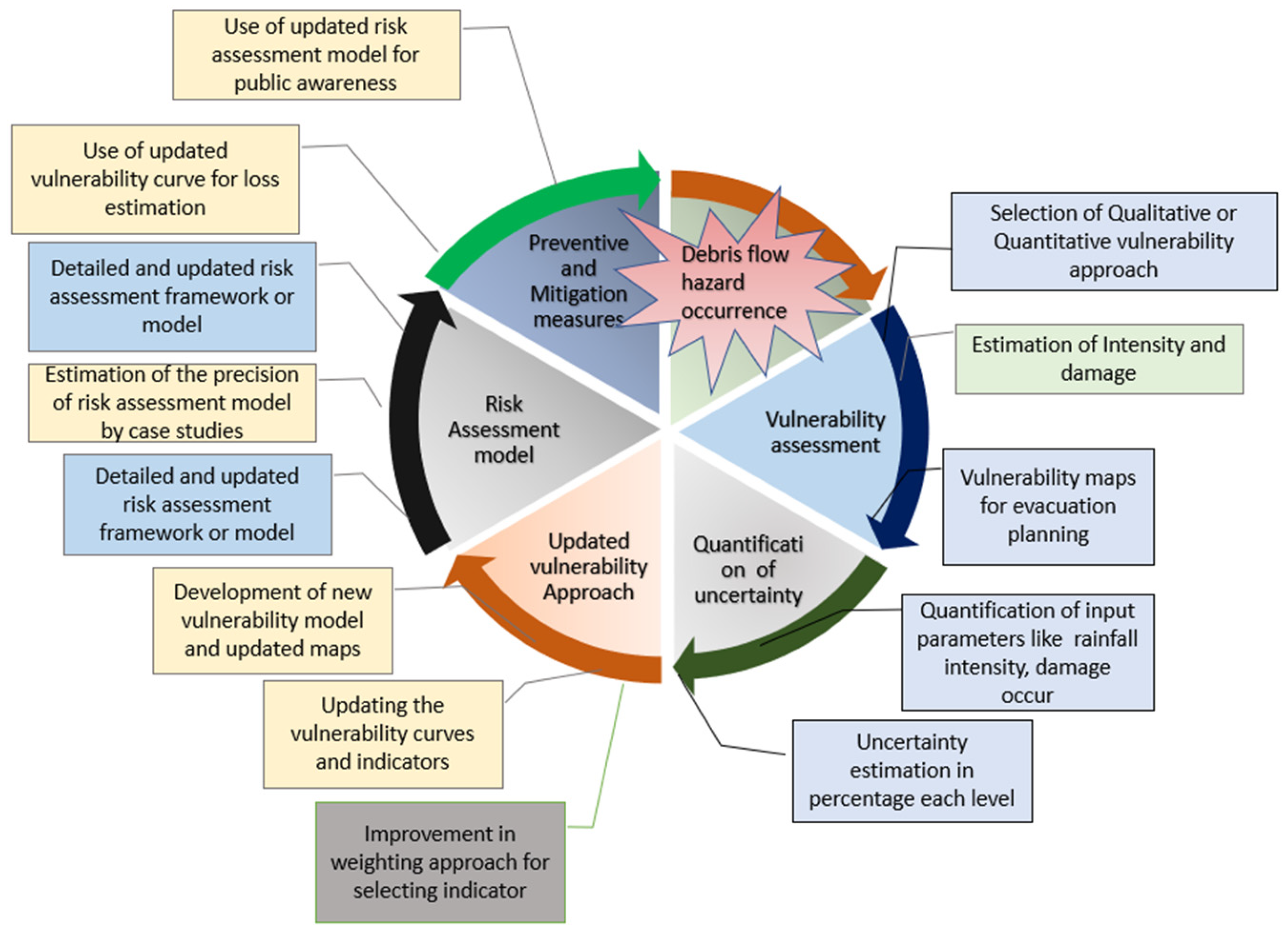
5. Recent Advancements in Vulnerability Assessment

A reliable risk management system requires the precise estimation of vulnerability to design better risk reduction strategies. Vulnerability further depends on accurate estimation of the intensity and damage by taking care of the uncertainties at each level [49,83,102]. These exercises will help to develop a more robust risk management framework that supports the decision-maker and stakeholders. The review of current studies provides the existing knowledge in the field of vulnerability assessment, with certain gaps to be filled to improve the way physical vulnerability is assessed. There is always room for improving the risk assessment strategy by updating computational aids and platforms. A new and updated vulnerability framework can be developed after incorporating the uncertainties verified by the well-documented case studies and by integrating the different approaches to complement each other, as described in Figure 10. Mitigation measures and early warning systems have also been revised to improve the risk assessment system.

Natural hazard scientists, practitioners, civil protection officers, and researchers continuously improve the existing vulnerability techniques by developing applications, codes, and software to collect more data for better risk estimation. In addition, many efforts are underway to understand, analyze, calculate and, if possible, visualize the vulnerability [103]. In this regard following recent progress has been made:

• Development of the advanced vulnerability function to assess the vulnerability quantitatively by correlating intensity along the (X-axis) with the building’s state of damage (Y-axis).
• Damage assessment has improved by determining property value based on market studies, reconstruction values, insurance companies, tax offices, and technical reports based on the size and type of buildings [104,105].
• Bahler et al., 2001 [106] initiated the "Pragmatic approach" based on the past existing data, local experience of the practitioner, expert judgment, and regional representative of the population for risk estimation of natural hazards. Furthermore, Swiss federal offices for civil protection and the environment developed an e-learning platform using a pragmatic approach. This software provides the calculation tools for simplified risk analysis in Switzerland and abroad.
• New vulnerability functions have been proposed by the researchers [28,45,107] based on the regression analysis using the Weibull approach for brick and reinforced brick structures.
• Recently, the MOVE vulnerability assessment framework has been developed by the FP7 MOVE Project engineers to address the vulnerability in a multidimensional view with respect to space and time.

6. Conclusions

Recent studies on mountainous hazards have attracted the attention of scholars and scientists toward the significance of physical vulnerability assessment in risk management systems. Debris movement is seen to have a remarkable impact on both human lives and the built environment. This review compared various vulnerability approaches in risk assessment systems and their associated uncertainties. From the critical analysis of pertinent literature, it has been concluded that vulnerability matrices, curves, and indicators are important approaches to estimating a structure’s vulnerability. However, their strengths and weaknesses clearly show a gap in enhancing vulnerability assessment approaches. Depositional height (h) from 0 to 6 m, impact pressure (p) ranges 0–35 kPa, and velocity (v) range 0–10 m/s are processed intensities responsible for the slight to complete destruction of residential buildings reported in the literature. Integration of vulnerability indicators with curves widens the vulnerability scope by considering different characteristics of buildings and intensity in vulnerability frameworks. Apart from that, land use patterns and better implementation of building standard codes with local adaptation measures may reduce the risk of building vulnerability to debris flow hazards. Furthermore, large data sets also consistently support vulnerability techniques; nonetheless, lack of data remains the main source of uncertainties in the risk management system. In addition, the interaction of elements at risk with debris flow requires extensive research, resulting in more comprehensive vulnerability strategies. Due to the direct loss of human life, most of the vulnerability strategy developed to date is only relevant to buildings. However, other structures such as retaining walls, bridge piers, highways, railways, and pipelines are also always threatened by mountainous hazards, but very few studies are available for these infrastructures. Finally, advancing uncertainties quantification techniques, especially in vulnerability matrices and indicators to make the risk reduction system more reliable, is a challenging gap to improve the vulnerability assessment system.

References

1. Jakob, M. Chapter 14—Landslides in a changing climate. In Hazards and Disasters Series; Davies, T., Rosser, N., Eds.; Elsevier: Amsterdam, The Netherlands, 2022; pp. 505–579. ISBN 978-0-12-818464-6. [Google Scholar]
2. Santi, P.M.; Hewitt, K.; VanDine, D.F.; Cruz, E.B. Debris-Flow Impact, Vulnerability, and Response. Nat. Hazards 2011, 56, 371–402. [Google Scholar] [CrossRef]
3. Dilley, M. Natural Disaster Hotspots: A Global Risk Analysis; World Bank Publications: Herndon, VA, USA, 2005; Volume 5, ISBN 0821359304. [Google Scholar]
4. Petley, D. Global Patterns of Loss of Life from Landslides. Geology 2012, 40, 927–930. [Google Scholar] [CrossRef]
5. Froude, M.J.; Petley, D.N. Global Fatal Landslide Occurrence from 2004 to 2016. Nat. Hazards Earth Syst. Sci. 2018, 18, 2161–2181. [Google Scholar] [CrossRef] [Green Version]
6. Dowling, C.A.; Santi, P.M. Debris Flows and Their Toll on Human Life: A Global Analysis of Debris-Flow Fatalities from 1950 to 2011. Nat. Hazards 2014, 71, 203–227. [Google Scholar] [CrossRef]
7. Ahmad, A.; Sutanto, M.H.; Harahap, I.S.H.; Al-Bared, M.A.M.; Khan, M.A. Feasibility of Demolished Concrete and Scraped Tires in Peat Stabilization—A Review on the Sustainable Approach in Stabilization. In Proceedings of the 2020 2nd International Sustainability and Resilience Conference: Technology and Innovation in Building Designs, Sakheer, Bahrain, 11–12 November 2020. [Google Scholar] [CrossRef]
8. Lee, S.G.; Winter, M.G. The Effects of Debris Flow in the Republic of Korea and Some Issues for Successful Risk Reduction. Eng. Geol. 2019, 251, 172. [Google Scholar] [CrossRef]
9. Reports, U.S. Geological Survey, USGS Science for Changing World. 2018. Available online: htpps://www.usgs.gov/faqs/how-many-deaths-result-each-year (accessed on 25 July 2022).
10. Thouret, J.C.; Antoine, S.; Magill, C.; Ollier, C. Lahars and Debris Flows: Characteristics and Impacts. Earth-Sci. Rev. 2020, 201, 103003. [Google Scholar] [CrossRef]
11. Nikolopoulos, E.I.; Crema, S.; Marchi, L.; Marra, F.; Guzzetti, F.; Borga, M. Impact of Uncertainty in Rainfall Estimation on the Identification of Rainfall Thresholds for Debris Flow Occurrence. Geomorphology 2014, 221, 286–297. [Google Scholar] [CrossRef]
12. Hakro, M.R.; Harahap, I.S.H. Flume Experiments for Investigation of Rainfall-Induced Slope Failure. Int. J. Eng. Res. Afr. 2015, 16, 49–56. [Google Scholar] [CrossRef]
13. Ibrahim, M.B.; Mustaffa, Z.; Balogun, A.L.; Hamonangan Harahap, I.S.; Ali Khan, M. Advanced Data Mining Techniques for Landslide Susceptibility Mapping. Geomat. Nat. Hazards Risk 2021, 12, 2430–2461. [Google Scholar] [CrossRef]
14. Cannon, S.H.; Gartner, J.E.; Rupert, M.G.; Michael, J.A.; Rea, A.H.; Parrett, C. Predicting the Probability and Volume of Postwildfire Debris Flows in the Intermountain Western United States. Bull. Geol. Soc. Am. 2010, 122, 127–144. [Google Scholar] [CrossRef]
15. Du, J.; Yin, K.; Lacasse, S.; Nadim, F. Quantitative Vulnerability Estimation of Structures for Individual Landslide: Application to the Metropolitan Area of San Salvador, El Salvador. J. Softw. Eng. 2015, 9, 1251–1264. [Google Scholar]
16. Shanmugam, G.; Alderton, D.; Elias, S.A. (Eds.) Deep-Water Processes and Deposits; Academic Press: Oxford, UK, 2021; pp. 965–1009. ISBN 978-0-08-102909-1. [Google Scholar]
17. Khan, M.A.; Mustaffa, Z.; Balogun, A.L.B.; Al-Bared, M.A.M.; Ahmad, A. Role of the Rheological Parameters in Debris Flow Modelling. IOP Conf. Ser. Mater. Sci. Eng. 2021, 1092, 012041. [Google Scholar] [CrossRef]
18. Iverson, R.M. The Debris-Flow Rheology Myth. Int. Conf. Debris-Flow Hazards Mitig. Mech. Predict. Assess. Proc. 2003, 1, 303–314. [Google Scholar]
19. Iverson, R.M.; Reid, M.E.; Lahusen, R.G. Debris-Flow Mobilisation. Annu. Rev. Earth Planet Sci. 1997, 25, 85–138. [Google Scholar] [CrossRef]
20. Jakob, M. Debrisow hazard analysis. In Debris-Flow Hazards and Related Phenomena; Springer: Berlin/Heidelberg, Germany, 2005. [Google Scholar]
21. Varnes, J.; Cruden, M. Chapter 3—Landslide types and process. In Landslides: Investigation and Mitigation; Transportation Research Boar: Washington, DC, USA, 1996. [Google Scholar]
22. Lee, E.M. Landslide Risk Assessment: The Challenge of Estimating the Probability of Landsliding. Q. J. Eng. Geol. Hydrogeol. 2009, 42, 445–458. [Google Scholar] [CrossRef]
23. Gartner, J.E.; Jakob, M. Debris-Flow Risk Assessment and Mitigation Design for Pipelines in British Columbia, Canada. In Proceedings of the 7th International Conference on Debris-Flow Hazards Mitigation, Golden, CO, USA, 10–13 June 2019; pp. 677–684. [Google Scholar]
24. Michael-Leiba, M.; Baynes, F.; Scott, G.; Granger, K. Quantitative Landslide Risk Assessment of Cairns, Australia. In Landslide Hazard and Risk; Glade, T., Anderson, M.G., Crozier, M.J., Eds.; Wiley: London, UK, 2005; pp. 621–642. [Google Scholar]
25. Birkmann, J.; Cardona, O.D.; Carreño, M.L.; Barbat, A.H.; Pelling, M.; Schneiderbauer, S.; Kienberger, S.; Keiler, M.; Alexander, D.; Zeil, P.; et al. Framing Vulnerability, Risk and Societal Responses: The MOVE Framework. Nat. Hazards 2013, 67, 193–211. [Google Scholar] [CrossRef]
26. Vamvatsikos, D.; Kouris, L.A.; Panagopoulos, G.; Kappos, A.J.; Nigro, E.; Rossetto, T.; Lloyd, T.O.; Stathopoulos, T. Structural Vulnerability Assessment under Natural Hazards: A Review. In COST ACTION C26: Urban Habitat Constructions under Catastrophic Events—Proceedings of the Final Conference; Taylor & Francis Group: London, UK, 2010; pp. 711–723. ISBN 978-0-415-60685-1. [Google Scholar]
27. Papathoma-Köhle, M.; Gems, B.; Sturm, M.; Fuchs, S. Matrices, Curves and Indicators: A Review of Approaches to Assess Physical Vulnerability to Debris Flows. Earth-Sci. Rev. 2017, 171, 272–288. [Google Scholar] [CrossRef]
28. Totschnig, R.; Fuchs, S. Mountain Torrents: Quantifying Vulnerability and Assessing Uncertainties. Eng. Geol. 2013, 155, 31–44. [Google Scholar] [CrossRef] [Green Version]
29. Wu, Y.; Li, J. Finite Element Analysis on Mechanical Behavior of Semi-Exposed Pipeline Subjected to Debris Flows. Eng. Fail. Anal. 2019, 105, 781–797. [Google Scholar] [CrossRef]
30. Pierson, T.C.; Costa, J.E.; Vancouver, W. A rheologic classification of subaerial sediment-water flows. In Debris Flow/Avalanches: Process, Recognition, and Mitigation; Geological Society of America: Boulder, CO, USA, 1987; Volume 7, pp. 1–12. [Google Scholar]
31. Hürlimann, M.; Coviello, V.; Bel, C.; Guo, X.; Berti, M.; Graf, C.; Hübl, J.; Miyata, S.; Smith, J.B.; Yin, H.Y. Debris-Flow Monitoring and Warning: Review and Examples. Earth-Sci. Rev. 2019, 199. [Google Scholar] [CrossRef]
32. Pierson, T.C. Important Process in High Country Gully Erosion. J. Tussock Grassl. Mt. Lands Inst. 1980, 3–14. [Google Scholar]
33. Amaral, G.; Bushee, J.; Cordani, U.G.; Kawashita, K.; Reynolds, J.H.; Almeida, F.F.M.; de Almeida, F.F.M.; Hasui, Y.; de Brito Neves, B.B.; Fuck, R.A.; et al. A Review of the Classifcation of Landslide of the Flow Type. J. Petrol. 2013, 369, 1689–1699. [Google Scholar] [CrossRef]
34. Castelli, F.; Freni, G.; Lentini, V.; Fichera, A. Modelling of a Debris Flow Event in the Enna Area for Hazard Assessment. Procedia Eng. 2017, 175, 287–292. [Google Scholar] [CrossRef]
35. Innes, J.L. Debris Flows. Prog. Phys. Geogr. 1983, 7, 469–501. [Google Scholar] [CrossRef]
36. Wells, W. Debris Flows/Avalanches. Geol. Soc. Am. 1987, 7, 105–114. [Google Scholar]
37. Petrović, N. Climate Change and Landslide Hazard. Annu. Disaster Risk Sci. 2018, 1, 3–18. [Google Scholar]
38. Tohari, A. Study of rainfall-induced landslide: A review. IOP Conf. Ser.: Earth Environ. Sci. 2018, 118, 012036. [Google Scholar] [CrossRef]
39. Turner, K.A.; Schuster, R.L. Landslides Investigation and Mitigation Report by NRC United State; Transportation Research Board: Washington, DC, USA, 2022. [Google Scholar]
40. Reid, M.E.; Iverson, R.M.; Logan, M.; Lahusen, R.G.; Godt, J.W.; Griswold, J.P. Entrainment of Bed Sediment by Debris Flows: Results from Large-Scale Experiments. Ital. J. Eng. Geol. Environ. 2011, 367–374. [Google Scholar] [CrossRef]
41. Wang, Y.; Liu, X.; Yao, C.; Li, Y. Debris-Flow Impact on Piers with Different Cross-Sectional Shapes. J. Hydraul. Eng. 2020, 146, 04019045. [Google Scholar] [CrossRef]
42. Eu, S.; Im, S.; Kim, D. Development of Debris Flow Impact Force Models Based on Flume Experiments for Design Criteria of Soil Erosion Control Dam. Adv. Civ. Eng. 2019, 2019, 3567374. [Google Scholar] [CrossRef]
43. Schuster, R.L.; Salcedo, D.A.; Valenzuela, L. Overview of Catastrophic Landslides of South America in the Twentieth Century. Rev. Eng. Geol. 2002, 15, 1–34. [Google Scholar]
44. Papathoma-Köhle, M.; Kappes, M.; Keiler, M.; Glade, T. Physical Vulnerability Assessment for Alpine Hazards: State of the Art and Future Needs. Nat. Hazadrs 2011, 58, 645–657. [Google Scholar] [CrossRef]
45. Fuchs, S.; Ornetsmüller, C.; Totschnig, R. Spatial Scan Statistics in Vulnerability Assessment: An Application to Mountain Hazards. Nat. Hazards 2012, 64, 2129–2151. [Google Scholar] [CrossRef] [Green Version]
46. Yiğit, A.; Lav, M.A.; Gedikli, A. Vulnerability of Natural Gas Pipelines under Earthquake Effects. J. Pipeline Syst. Eng. Pract. 2018, 9, 1–14. [Google Scholar] [CrossRef]
47. Leone, F.; Asté, J.-P.; Velasquez, E. Contribution Des Constats d’endommagement Au Développement d’une Méthodologie d’évaluation de La Vulnérabilité Appliquée Aux Phénomènes de Mouvements de Terrain (Contribution of Damaging Reports to the Development of an Appraisal Methodology of Vulnerabil. Bull. L’Assoc. Géogr. Fr. 1995, 72, 350–371. [Google Scholar] [CrossRef]
48. Huggel, C.; Allen, S.; Deline, P.; Fischer, L.; Noetzli, J.; Ravanel, L. Ice Thawing, Mountains Falling—Are Alpine Rock Slope Failures Increasing? Geol. Today 2012, 28, 98–104. [Google Scholar] [CrossRef]
49. Akbas, S.O.; Blahut, J.; Sterlacchini, S. Critical assessment of existing physical vulnerability estimation approaches for debris flows. Proc. Landslide Process. Geomorphol. Mapp. Dyn. Model. 2009, 67, 229–233. [Google Scholar]
50. Zhang, S.; Zhang, L.; Li, X.; Xu, Q. Physical Vulnerability Models for Assessing Building Damage by Debris Flows. Eng. Geol. 2018, 247, 145–158. [Google Scholar] [CrossRef]
51. Birkmann, J. Chapter 2—Indicators and Criteria for Measuring Vulnerability: Theoretical Bases and Requirements. In Measuring Vulnerability to Natural Hazards: Towards Disaster Resilient Societies, 2nd ed.; United Nation University Press: Tokyo, Japan, 2013; pp. 55–77. [Google Scholar]
52. Papathoma-Köhle, M.; Keiler, M.; Totschnig, R.; Glade, T. Improvement of Vulnerability Curves Using Data from Extreme Events: Debris Flow Event in South Tyrol. Nat. Hazards 2012, 64, 2083–2105. [Google Scholar] [CrossRef]
53. Thouret, J.C.; Ettinger, S.; Guitton, M.; Santoni, O.; Magill, C.; Martelli, K.; Zuccaro, G.; Revilla, V.; Charca, J.A.; Arguedas, A. Assessing Physical Vulnerability in Large Cities Exposed to Flash Floods and Debris Flows: The Case of Arequipa (Peru). Nat. Hazards 2014, 73, 1771–1815. [Google Scholar] [CrossRef]
54. Godfrey, A.; Ciurean, R.L.; Van Westen, C.J.; Kingma, N.C.; Glade, T. Assessing Vulnerability of Buildings to Hydro-Meteorological Hazards Using an Expert Based Approach–An Application in Nehoiu Valley, Romania. Int. J. Disaster Risk Reduct. 2015, 13, 229–241. [Google Scholar] [CrossRef]
55. Fuchs, S.; Heiss, K.; Hübl, J. Towards an Empirical Vulnerability Function for Use in Debris Flow Risk Assessment. Nat. Hazards Earth Syst. Sci. 2007, 7, 495–506. [Google Scholar] [CrossRef] [Green Version]
56. Rossetto, T.; Ioannou, I.; Grant, D.; Maqsood, T. Guidelines for the Empirical Vulnerability Assessment. GEM Tech. Rep. 2014, 8, 140. [Google Scholar]
57. Westen, C.J.V. Vulnerability Role in Disaster Management (Report). In CHARIM. 2020, pp. 1–8. Available online: www.charim.net (accessed on 25 February 2022).
58. FEMA Hazus Flood Model User Guidance. Hazus User Guidance & Technical Manuals. U.S. Department of Homeland Security. 2018; p. 263. Available online: www.fema.gov (accessed on 20 April 2022).
59. Zanchetta, G.; Sulpizio, R.; Pareschi, M.T.; Leoni, F.M.; Santacroce, R. Characteristics of 5–6 May 1998 Volcaniclastic Debris Flows in the Sarno Area (Campania, Southern Italy): Relationships to Structural Damage and Hazard Zonation. J. Volcanol. Geotherm. Res. 2004, 133, 377–393. [Google Scholar] [CrossRef]
60. Hu, K.H.; Cui, P.; Zhang, J.Q. Characteristics of Damage to Buildings by Debris Flows on 7 August 2010 in Zhouqu, Western China. Nat. Hazards Earth Syst. Sci. 2012, 12, 2209–2217. [Google Scholar] [CrossRef]
61. Jakob, M.; Stein, D.; Ulmi, M. Vulnerability of Buildings to Debris Flow Impact. Nat. Hazards 2012, 60, 241–261. [Google Scholar] [CrossRef]
62. Winter, M.; Smith, J.; Fotopoulou, S.; Pitilakis, K.; Mavrouli, O.; Corominas, J.; Agyroudis, S. The Physical Vulnerability of Roads to Debris Flow. In Proceedings of the 18th International Conference on Soil Mechanics and Geotechnical Engineering, Paris, France, 2–6 September 2013; pp. 307–313. [Google Scholar]
63. Kang, H.; Kim, Y. The Physical Vulnerability of Different Types of Building Structure to Debris Flow Events. Nat. Hazards 2016, 80, 1475–1493. [Google Scholar] [CrossRef]
64. Haugen, E.D.; Kaynia, A.M. Vulnerability of Structures Impacted by Debris Flow. In Landslides and Engineered Slopes; Taylor & Francis: London, UK, 2008; pp. 381–387. [Google Scholar]
65. Quan Luna, B.; Blahut, J.; Van Westen, C.J.; Sterlacchini, S.; Van Asch, T.W.J.; Akbas, S.O. The Application of Numerical Debris Flow Modelling for the Generation of Physical Vulnerability Curves. Nat. Hazards Earth Syst. Sci. 2011, 11, 2047–2060. [Google Scholar] [CrossRef] [Green Version]
66. Quan Luna, B.; Blahut, J.; Camera, C.; van Westen, C.; Apuani, T.; Jetten, V.; Sterlacchini, S. Physically Based Dynamic Run-out Modelling for Quantitative Debris Flow Risk Assessment: A Case Study in Tresenda, Northern Italy. Environ. Earth Sci. 2014, 72, 645–661. [Google Scholar] [CrossRef]
67. Ciurean, R.L.; Hussin, H.; van Westen, C.J.; Jaboyedoff, M.; Nicolet, P.; Chen, L.; Frigerio, S.; Glade, T. Multi-Scale Debris Flow Vulnerability Assessment and Direct Loss Estimation of Buildings in the Eastern Italian Alps. Nat. Hazards 2017, 85, 929–957. [Google Scholar] [CrossRef] [Green Version]
68. Shen, P.; Zhang, L.; Chen, H.; Fan, R. EDDA 2.0: Integrated Simulation of Debris Flow Initiation and Dynamics Considering Two Initiation Mechanisms. Geosci. Model Dev. 2018, 11, 2841–2856. [Google Scholar] [CrossRef] [Green Version]
69. Yan, S.; He, S.; Deng, Y.; Liu, W.; Wang, D.; Shen, F. A Reliability-Based Approach for the Impact Vulnerability Assessment of Bridge Piers Subjected to Debris Flows. Eng. Geol. 2020, 269, 105567. [Google Scholar] [CrossRef]
70. Kappes, M.S.; Papathoma-Koehle, M.; Keiler, M. Assessing Physical Vulnerability for Multi-Hazards Using an Indicator-Based Methodology. Appl. Geogr. 2012, 32, 577–590. [Google Scholar] [CrossRef]
71. Dadfar, B.; El Naggar, M.H.; Nastev, M. Vulnerability of Buried Energy Pipelines Subject to Earthquake-Triggered Transverse Landslides in Permafrost Thawing Slopes. J. Pipeline Syst. Eng. Pract. 2018, 9, 1–12. [Google Scholar] [CrossRef]
72. Mustaffa, Z.; Al-Bared, M.A.M.; Habeeb, N.; Khan, M.A. Examining the Effect of Debris Flow on Oil and Gas Pipelines Using Numerical Analysis. Glob. J. Earth Sci. Eng. 2022, 9, 74–87. [Google Scholar] [CrossRef]
73. Leone, F.; Asté, J.P.; Leroi, E. Vulnerability Assessment of Elements Exposed to Mass-Movement: Working toward a Better Risk Perception. In Landslides, Glissements de Terrain; Senneset, K., Ed.; Balkema: Rotterdam, The Netherlands, 1996; pp. 263–270. [Google Scholar]
74. Leone, F.; Asté, J.-P.; Leroi, E. L’évaluation de La Vulnérabilité Aux Mouvements de Terrains: Pour Une Meilleure Quantification Du Risque/The Evaluation of Vulnerability to Mass Movements: Towards a Better Quantification of Landslide Risks. Rev. Géogr. Alp. 1997, 84, 35–46. [Google Scholar] [CrossRef]
75. Ouyang, C.; Wang, Z.; An, H.; Liu, X.; Wang, D. An Example of a Hazard and Risk Assessment for Debris Flows—A Case Study of Niwan Gully, Wudu, China. Eng. Geol. 2019, 263, 105351. [Google Scholar] [CrossRef]
76. Delannay, R.; Valance, A.; Mangeney, A.; Roche, O.; Richard, P. Granular and Particle-Laden Flows: From Laboratory Experiments to Field Observations. J. Phys. D Appl. Phys. 2017, 50, 053001. [Google Scholar] [CrossRef]
77. Han, Z.; Su, B.; Li, Y.; Wang, W.; Wang, W.; Huang, J.; Chen, G. Numerical Simulation of Debris-Flow Behavior Based on the SPH Method Incorporating the Herschel-Bulkley-Papanastasiou Rheology Model. Eng. Geol. 2019, 255, 26–36. [Google Scholar] [CrossRef]
78. Shimizu, H.A.; Koyaguchi, T.; Suzuki, Y.J. A Numerical Shallow-Water Model for Gravity Currents for a Wide Range of Density Differences. Prog. Earth Planet. Sci. 2017, 4, 8. [Google Scholar] [CrossRef] [Green Version]
79. Gao, L.; Zhang, L.M.; Chen, H.X.; Shen, P. Simulating Debris Fl Ow Mobility in Urban Settings. Eng. Geol. 2016, 214, 67–78. [Google Scholar] [CrossRef]
80. Christen, M.; Kowalski, J.; Bartelt, P. RAMMS: Numerical Simulation of Dense Snow Avalanches in Three-Dimensional Terrain. Cold Reg. Sci. Technol. 2010, 63, 1–14. [Google Scholar] [CrossRef] [Green Version]
81. Gregoretti, C.; Degetto, M.; Boreggio, M. GIS-Based Cell Model for Simulating Debris Flow Runout on a Fan. J. Hydrol. 2016, 534, 326–340. [Google Scholar] [CrossRef]
82. Azmeri, A.; Isa, A.H. An Analysis of Physical Vulnerability to Flash Floods in the Small Mountainous Watershed of Aceh Besar Regency, Aceh Province, Indonesia. Jàmbá: J. Disaster Risk Stud. 2018, 10, 1–6. [Google Scholar] [CrossRef] [PubMed] [Green Version]
83. Fuchs, S.; Keiler, M.; Ortlepp, R.; Schinke, R.; Papathoma-Köhle, M. Recent Advances in Vulnerability Assessment for the Built Environment Exposed to Torrential Hazards: Challenges and the Way Forward. J. Hydrol. 2019, 575, 587–595. [Google Scholar] [CrossRef]
84. Karagiorgos, K.; Heiser, M.; Thaler, T.; Hübl, J.; Fuchs, S. Micro-Sized Enterprises: Vulnerability to Flash Floods. Nat. Hazards 2016, 84, 1091–1107. [Google Scholar] [CrossRef] [Green Version]
85. Ronold, B.K.O.; Bjerager, P. Model Uncertainty Representation in Geotechnical Reliability Analyses. J. Geotech. Eng. 1992, 118, 363–376. [Google Scholar] [CrossRef]
86. Papathoma-Köhle, M.; Schlögl, M.; Fuchs, S. Vulnerability Indicators for Natural Hazards: An Innovative Selection and Weighting Approach. Sci. Rep. 2019, 9, 1–14. [Google Scholar] [CrossRef] [Green Version]
87. Ettinger, S.; Mounaud, L.; Magill, C.; Yao-Lafourcade, A.F.; Thouret, J.C.; Manville, V.; Negulescu, C.; Zuccaro, G.; De Gregorio, D.; Nardone, S.; et al. Building Vulnerability to Hydro-Geomorphic Hazards: Estimating Damage Probability from Qualitative Vulnerability Assessment Using Logistic Regression. J. Hydrol. 2016, 541, 563–581. [Google Scholar] [CrossRef]
88. Eidsvig, U.M.K.; Papathoma-Köhle, M.; Du, J.; Glade, T.; Vangelsten, B.V. Quantification of Model Uncertainty in Debris Flow Vulnerability Assessment. Eng. Geol. 2014, 181, 15–26. [Google Scholar] [CrossRef]
89. Ciurean, R.L.; Schröter, D.; Glade, T. Conceptual Frameworks of Vulnerability Assessments for Natural Disasters Reduction; InTech: Saitama-shi, Japan, 2013. [Google Scholar]
90. Uzielli, M.; Nadim, F.; Lacasse, S.; Kaynia, A.M. A Conceptual Framework for Quantitative Estimation of Physical Vulnerability to Landslides. Eng. Geol. 2008, 102, 251–256. [Google Scholar] [CrossRef]
91. Kaynia, A.M.; Papathoma-Köhle, M.; Neuhäuser, B.; Ratzinger, K.; Wenzel, H.; Medina-Cetina, Z. Probabilistic Assessment of Vulnerability to Landslide: Application to the Village of Lichtenstein, Baden-Württemberg, Germany. Eng. Geol. 2008, 101, 33–48. [Google Scholar] [CrossRef]
92. Uzielli, M.; Lacasse, S.; Nadim, F. Probabilistic Risk Estimation for Geohazards: A Simulation Approach. In Proceedings of the International Symposium on Geotechnical Safety and Risk; CRC Press: Boca Raton, FL, USA, 2009; pp. 355–362. [Google Scholar]
93. Gong, W.; Gupta, H.V.; Yang, D.; Sricharan, K.; Hero, A.O. Estimating Epistemic and Aleatory Uncertainties during Hydrologic Modeling: An Information Theoretic Approach. Water Resour. Res. 2013, 49, 2253–2273. [Google Scholar] [CrossRef] [Green Version]
94. Li, Z.; Nadim, F.; Huang, H.; Uzielli, M.; Lacasse, S. Quantitative Vulnerability Estimation for Scenario-Based Landslide Hazards. Landslides 2010, 7, 125–134. [Google Scholar] [CrossRef]
95. Liang, W.; Zhuang, D.; Jiang, D.; Pan, J.; Ren, H. Assessment of Debris Flow Hazards Using a Bayesian Network. Geomorphology 2012, 171–172, 94–100. [Google Scholar] [CrossRef]
96. Reckhow, K.H. Water Quality Prediction and Probability Network Models. Can. J. Fish. Aquat. Sci. 1999, 56, 1150–1158. [Google Scholar] [CrossRef]
97. Uzielli, M. Risk and Vulnerability for Geohazards—Probabilistic Estimation of Regional Vulnerability to Landslides. In Proceedings of the 13th Panamerican Conference on Soil Mechanics and Geotechnical Engineering at Margarita, Porlamar, Venezuela, 16–20 July 2007. [Google Scholar]
98. Papadopoulos, C.E.; Yeung, H. Uncertainty Estimation and Monte Carlo Simulation Method. Flow Meas. Instrum. 2001, 12, 291–298. [Google Scholar] [CrossRef]
99. Khalaj, S.; BahooToroody, F.; Mahdi Abaei, M.; BahooToroody, A.; De Carlo, F.; Abbassi, R. A Methodology for Uncertainty Analysis of Landslides Triggered by an Earthquake. Comput. Geotech. 2020, 117, 103262. [Google Scholar] [CrossRef]
100. Christian, J.T. Geotechnical Engineering Reliability: How Well Do We Know What We Are Doing? J. Geotech. Geoenvironmental Eng. 2004, 130, 985–1003. [Google Scholar] [CrossRef]
101. Zhang, J.; Tang, W.H.; Zhang, L.M.; Huang, H.W. Characterising Geotechnical Model Uncertainty by Hybrid Markov Chain Monte Carlo Simulation. Comput. Geotech. 2012, 43, 26–36. [Google Scholar] [CrossRef]
102. Wei, Z.; Xu, Y.P.; Sun, H.; Xie, W.; Wu, G. Predicting the Occurrence of Channelized Debris Flow by an Integrated Cascading Model: A Case Study of a Small Debris Flow-Prone Catchment in Zhejiang Province, China. Geomorphology 2018, 308, 78–90. [Google Scholar] [CrossRef]
103. Fuchs, S.; Thaler, T. Vulnerability and Resilience to Natural Hazards; Cambridge University Press: Cambridge, UK, 2018; ISBN 1107154898. [Google Scholar]
104. Fuchs, S.; Keiler, M.; Zischg, A. A Spatiotemporal Multi-Hazard Exposure Assessment Based on Property Data. Nat. Hazards Earth Syst. Sci. 2015, 15, 2127–2142. [Google Scholar] [CrossRef] [Green Version]
105. Röthlisberger, V.; Zischg, A.P.; Keiler, M. A Comparison of Building Value Models for Flood Risk Analysis. Nat. Hazards Earth Syst. Sci. 2018, 18, 2431–2453. [Google Scholar] [CrossRef] [Green Version]
106. Bähler, F.; Wegmann, M.; Merz, H. Pragmatischer Ansatz Zur Risikobeurteilung von Naturgefahren. Wasser Energ. Luft 2001, 93, 193–196. [Google Scholar]
107. Totschnig, R.; Sedlacek, W.; Fuchs, S. A Quantitative Vulnerability Function for Fluvial Sediment Transport. Nat. Hazards 2011, 58, 681–703. [Google Scholar] [CrossRef]
Figure 1. Illustration of debris flow process and impact on infrastructure.
Land 11 02240 g001
Figure 2. A bibliographic representation of the countries contributing to the physical vulnerability assessment research of debris flow hazards in the last 20 years (Vos viewer).
Land 11 02240 g002
Figure 3. Different types of physical vulnerability approach.
Land 11 02240 g003
Figure 4. The minimum number of information required for an empirical database [56].
Land 11 02240 g004
Figure 5. Structural vulnerability matrix [73].
Land 11 02240 g005
Figure 6. Comparison of the physical vulnerability curves [83].
Land 11 02240 g006
Figure 7. The conceptual methodology of the indicator-based approach for the building [70].
Land 11 02240 g007
Figure 8. Example of the vulnerability indicators is demonstrated together with the weight index and scores which can vary according to the objective of the study and the end-users [70].
Land 11 02240 g008
Figure 9. Process stage of uncertainties associated with vulnerability analysis [88].
Land 11 02240 g009
Figure 10. Risk management system showing various steps of analysis (reproduced and updated from [27]).
Land 11 02240 g010