Abstract
The aggravation of extreme weather events has dramatically increased the risk of severe water shortages and seriously threatened agricultural production. The Huang-Huai-Hai region, an important agricultural production region in China, is subject to a severe water shortage and is often hit by drought. As a result, water-saving technologies (WSTs) have been implemented. It remains unclear how effectively these WSTs can reduce crop yield loss, crop yield variation, and the loss of net crop income caused by water scarcity. Therefore, this paper aimed to analyze the role of WSTs in response to drought by establishing a multi-objective expected utility function based on 988 farmers across the Huang-Huai-Hai region. Econometric analysis employing an endogenous switching regression model showed that using WSTs can significantly reduce crop yield loss and net income loss caused by drought. Adopting household-based WSTs or community-based water-saving technology generates even greater positive effects on crop yield and farmers’ net income. Therefore, the government should promote farmers’ adoption of more advanced WSTs by increasing subsidies and strengthening policy support.
1. Introduction
The aggravation of extreme weather events has greatly increased the risk of severe water shortages and, therefore, seriously threatens agricultural production. According to statistics, 28–38% of global farmland faces total water scarcity [1]. Furthermore, it has been estimated that the global drought-affected area will increase from 15% to 44% by the end of the 21st century [2], and 11% (±5%) of global croplands are estimated to be vulnerable to projected climate-driven water scarcity by 2050 [3]. As one of the most water-scarce countries, China is facing increasing pressure on agricultural water supply. With the agricultural water scarcity index rising from 0.32 to 0.49 during 2000–2014 [4], water shortage has become the most threatening factor to China’s food security [5,6]. The Huang-Huai-Hai region, one of the most important grain-producing regions in China, faces severe water shortages all year round, with an agricultural water shortage index beyond 0.80 [4] and, on average, about 20% of the crop area suffering from severe water shortages every year [7]. As a result, during 2010–2019, the average annual crop income loss reached 26.39 million tons due to drought, and the crop loss rate reached 4.7% [8,9].
Therefore, how to alleviate the pressure of agricultural water shortage and adapt to drought have become hot topics. Israel and Australia, for instance, have become more resilient owing to notable success in drought risk management, achieved through improvements in water use practices and development of long-term water management plans [10]. Many studies have shown that adopting water-saving technologies (WSTs) can not only limit water waste, but also reduce agricultural water consumption by improving the efficiency of water utilization. For example, Belder et al. [11] found that adopting WSTs can reduce water consumption by 15% compared to traditional irrigation methods without affecting crop yield. Similarly, Huang et al. [12] and Vatta et al. [13] found that the use of WSTs can reduce agricultural water use and increase water productivity. Li et al. [14] and Zhai et al. [15] made a further step, finding that adopting new WSTs, such as drip irrigation and micro-sprinkler irrigation, improved the efficiency of water use and reduced water evapotranspiration at the same time. In addition, Guo et al. [16] found that the dry–wet alternate irrigation technique reduced total water consumption by 50.9% compared with continuous flooding irrigation.
As a result, promoting agricultural WST adoption has received increasing attention from government departments. In April 2009, the General Office of the State Council of China formulated the National Water-Saving Irrigation Plan. In 2015, the National Agricultural Sustainable Development Plan (2015–2030) issued by the Ministry of Agriculture of China emphasized the need to vigorously develop water-saving agriculture, promote water-saving irrigation, and increase the construction of water-saving irrigation projects in major grain-producing areas. According to the Chinese government’s requirements, China’s high-efficiency water-saving irrigation area reached over 19.2 million hectares by 2020, and, meanwhile, the effective irrigation ratio and water-saving irrigation ratio should reach 57% and 75%, respectively, by 2030. Statistics show that, in the past two decades (2001–2020), the water-saving irrigation area in China has increased steadily (from 17,466 thousand hectares to 37,796 thousand hectares), and the proportion of water-saving irrigation in the effective irrigation area has also increased from 32% to 55% [17] (Figure 1).
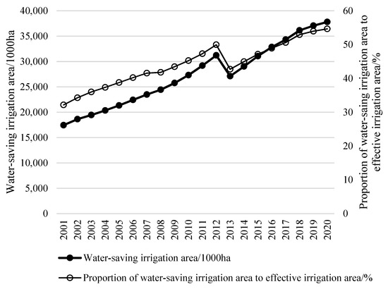
Figure 1.
The water-saving irrigation area and its proportion to the effective irrigation area in China (2001–2020).
Given that farmers are the direct decision-makers regarding adopting WSTs in response to drought, it is crucial to identify the factors that influence their willingness to adopt WSTs and to further analyze the efficiency of WSTs. However, most of the current literature mainly focuses on the impact mechanism of farmers’ adoption of WSTs, such as institutional and policy subsidies [18,19,20,21], financial and technological constraints [20,22,23], climate and land factors [18,24,25], and farmers’ social capital and household characteristics [6,26,27]. Only a few studies have analyzed the efficiency of WSTs in terms of water resource utilization and productivity, as well as irrigation frequency [12,15,16,28,29,30,31]. In addition, in previous studies identifying adaption measures to extreme weather events, researchers mainly considered farmland management measures and engineering irrigation measures [7,32,33,34,35,36,37], and few investigated whether WSTs can effectively address drought and offset drought risks.
To fill the gaps, this paper attempts to answer the following questions: What types of WSTs do farmers adopt to deal with drought? Can WSTs effectively adapt to drought? That is, does the use of WSTs reduce crop yield loss, crop yield variation, and net crop income loss? What are the different effects of different types of WSTs? This information and empirical results are useful for policymakers when they are making public irrigation investment in WSTs. To answer these questions, this paper accurately describes the adaptive behavior of farmers and analyzes the effects of WSTs in response to drought by establishing a multi-objective expected utility function of yield maximization, risk minimization, and profit maximization based on a large field survey dataset from the Huang-Huai-Hai region in China. This paper contributes to the literature in three ways: (i) a multi-objective expected utility model of crop yield, risk, and net income is established to analyze farmers’ behavior relating to adopting WSTs; (ii) an endogenous switching regression model is used to construct a simultaneous equation of farmers’ adaptation decision and effect of farmers adopting WSTs; and (iii) various types of WSTs are distinguished, and their effects are investigated.
The rest of this paper is organized as follows. The second part constructs a theoretical analysis framework and puts forward research hypotheses. The third part explains the data sources and establishes an empirical model according to the theoretical hypothesis. The fourth part discusses the estimated results and carries out specific analysis. The last part concludes.
2. Theoretical Basis and Analytical Framework
2.1. Adaptation Decisions of Farmers to Drought
Based on the assumption of complete information and drawing upon neoclassical economic theory, the decision-making model mainly proposes unilateral evaluation and analysis from the perspective of either consumers or producers, aiming to maximize the utility for consumers or the profit for producers, respectively. When based on the theoretical background of peasant economics, there is a certain possibility that farmers are both consumers and producers at the same time. In developing countries, farmers demonstrate the economic characteristics of self-sufficiency to a certain extent, as their agricultural products are not only sold in the market but also reserved for household consumption. Therefore, the farmers’ behavior is the result of a comprehensive decision that takes into consideration both production and consumption, as well as other factors [38]. Furthermore, production risk is a typical feature of agricultural sector, and unpredictable weather can pose serious difficulties and significant uncertainties to crop producers. Given harsh climatic and agroecological conditions, it is possible that food security can be threatened, or, worse, a famine is brought about. Without taking the risk of drought into consideration, it is difficult to accurately assess whether the decision-making behavior of farmers is risk averse [39]. Therefore, this paper aims to establish a production decision model for farmers who both produce and consume food when facing the risk of drought.
The economic behavior of farmers under uncertainty can be expressed as follows, according to Singh et al. [38]:
where represents the von Neumann–Morgenstern utility index, which is the preference of farmers facing risks. c1 is a part of the farmers’ crop production and consumption, and its price is p1; c2 is other products that farmers buy from the market, and their price is p2. is the crop production function, where y is the crop yield, x is an explanatory variable related to production, and v is an unpredictable random variable.
The budget restraint of farmers is , where m is the crop sales volume (market surplus), which satisfies the formula , that is, the crop production volume is composed of households’ own consumption and market sales. Furthermore, there is no sign limit for m; when the crop yield exceeds the consumption amount, the market surplus can be positive (m > 0); when the crop yield fails to reach the consumption amount, the market surplus is negative (m < 0). N(x) is the net income (net cost of x) of other farmer behaviors. According to , when assuming p2 = 1, the budget constraint can be converted into: .
Within the expected utility model, farmers need to make decisions to optimize the expected utility:
CE is the certainty equivalent, which means the utility level corresponding to the net income is equal to the expected utility level under uncertainty conditions, and the total income of farmers is , that is, it satisfies:
which is equivalent to:
The expected values of certainty and uncertainty may have different utilities for farmers, and the difference between them is the risk premium , which is the amount that farmers are willing to pay for avoiding the risks posed by drought. Considering the risk premium R, the following can be obtained:
When farmers are risk averse to drought, R > 0; then, the utility function of farmers’ income is a concave function, that is, , . As shown in Figure 2, when farmers face drought risk, they may profit in two different ways, namely, and , with probability and , respectively. Assuming the same income, the income utility (point A) of the farmers that face the drought risk is greater than the expected utility (point B) of the farmers that do not face such risk. Following this, in order to avoid the risk of climate change, farmers are willing to spend R to adopt relevant measures to deal with drought. At this time, the income utility of point B and point C is the same, that is, .
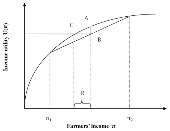
Figure 2.
The utility function of farmers being risk averse.
From the above analysis, this paper proposes:
Hypothesis 1.
Given that farmers are risk averse to drought, and other conditions remain unchanged, farmers cope with drought by adopting WSTs to reduce risk and ensure income. This means that drought may have a positive influence on farmers when they adopt the WSTs.
2.2. Effectiveness Analysis of WSTs
Many studies have testified that multi-objective utility theory has better accuracy in describing and predicting producer behaviors. Therefore, multi-objective utility theory models of farmers have recently gained attention [40,41,42]. In terms of crop production, the government is inclined to ensure food security from a macro perspective, while farmers are more concerned on how to reduce production risks and increase agricultural income from a micro perspective. In the face of climate changes, such as rising temperature, falling precipitation, and increasing drought, adopting WSTs can reduce the production risks and, thus, ensure crop yield and stabilize crop income, maximizing expected utility. Therefore, in the selection decision behavior of WSTs, we introduce three objective functions: yield maximization, income maximization, and risk minimization.
We establish a stochastic production function to analyze the marginal contribution of each factor to the average crop yield and yield risk. Two independent equations, and , represent average crop yield (the expectation of yield) and crop yield variation (the variance of yield), respectively. According to the generalized production function proposed by Just and Pope [43], the specific functional form is as follows:
A represents the behavior of adapting to drought. When A = 1, farmers adopt WSTs as adaptive measures (adopters), and, when A = 0, they do not adopt WSTs (non-adopters). X is the cost vector of production factors, and D is the occurrence of drought disasters. When D = 1, drought has occurred, and it is a drought year; when D = 0, it is a normal year. Both α and β are parameter vectors, and ε is the error term, which is assumed to obey the standard normal distribution ε~N(0,1).
Introducing the Just–Pope production function into the multi-objective utility function of farmers, the following is obtained:
where Py is the crop production cost, Px is the production factors cost, and PA is the cost of adopting WSTs. According to Equation (7), where the behavior of farmers in taking WST measures is discussed, the following research hypotheses can be made based on general economic theory.
Hypothesis 2.
WSTs are risk-reducing inputs, and adopters may reduce the negative impact of drought on the risk of crop production, that is,.
Hypothesis 3.
The average expected yield obtained by farmers adopting WSTs may be higher than that without adopting WSTs, that is,.
Hypothesis 4.
Farmers are in a perfectly competitive market, that is, they are the recipients of market prices (factor cost and agricultural production cost). Under the circumstance that the prices are all exogenously given, the net crop income obtained by farmers adopting WSTs is higher than that obtained without adopting WSTs.
3. Data and Descriptive
3.1. Data Sources
The Huang-Huai-Hai region is one of the most important grain-producing areas in China. This area is dominated by the double-cropping system of winter wheat and summer maize. The outputs of wheat and maize can reach 75% and 35% of the national total, respectively [8]. However, the crop output and farmers’ income in the region are not as promising as they should be due to the severe water shortage all the year round, the low water availability (1/7 of the national per capita), and the frequent extreme weather events such as drought. Therefore, it was of great significance to select the Huang-Huai-Hai region as the study area in this paper. Figure 3 shows the sample distribution across the Huang-Huai-Hai region.
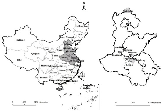
Figure 3.
Location of province and county samples across the Huang-Huai-Hai region.
This study conducted a large-scale questionnaire survey of villages and farmers across five provinces in China. A stratified random sampling method was used. First, several counties were selected in each province. The sampled counties had to meet the following two criteria: First, the county had to have suffered, at least once during 2010–2012, from a most severe or a severe drought, which indicates a drought disaster year. Second, the county had to have experienced at least one year of relatively normal weather during 2010–2012, which indicates a normal year. According to China’s national standard for natural disasters, natural disasters can be classified into four categories according to their severity: most severe, severe, moderate, and small [44]. A year is defined as a disaster year if the local government declares a disaster warning with a most severe or severe level; otherwise, it is a normal year. Next, three townships were randomly selected from each sample county. Townships were selected based on the infrastructure condition of irrigation and drainage, which was divided into three categories: good, medium, and poor. In each county, one township was selected for each category. Then, three villages were randomly selected in each selected township. At last, 10 farmers were randomly selected from each selected village to answer a questionnaire survey. The selected farmers were mainly engaged in crop production, and detailed interviews were carried out on the largest two plots of each farmer. According to the data processing, the total sample included five provinces, Henan, Hebei, Shandong, Anhui, and Jiangsu, 11 counties, 33 towns, 99 villages, 988 farmers, and 1880 plots (Table 1).

Table 1.
The distribution of sample farmers and plots across five provinces.
3.2. Sample Descriptive Analysis
3.2.1. Types of WST Uses
The survey data showed that farmers adopt various types of WSTs. If each WST was analyzed individually, the analysis process would be lengthy, and the results could be similar. Additionally, some WSTs were used at such a low rate that a separate analysis was not necessary. Therefore, this paper categorizes WSTs into three types: traditional WSTs, household-based WSTs, and community-based WSTs [12], based on the distinguishing characteristics of different WSTs, such as cost and service time, and referring to existing literature. Traditional WSTs include border irrigation, furrow irrigation, and land leveling. This type of technology has a long history and has been used since the 1950s. Moreover, traditional WSTs have low fixed costs and are labor intensive. Due to the small amount of arable land per capita in China, farmers can build furrows or level the land in just a few days. Household-based WSTs include seven major types: ground pipes (plastic pipes or water belts, etc.), plastic film mulching, no tillage/reduced tillage, straw mulching/returning to fields, chemicals, intermittent irrigation (alternating dry and wet irrigation), and drought-resistant varieties. These technologies have been used since the 1980s. Similar to traditional technologies, household-based WSTs are characterized by low fixed cost and high divisibility and are usually adopted by individual farmers. Community-based WSTs involve underground pipelines, sprinkler irrigation, drip irrigation, and channel seepage prevention. Compared to the first two types of technologies, the adoption of community-based WSTs was rather late. Due to the high investment cost, community-based WSTs often require collaboration within the community or the group work of farmers, and the divisibility is weak.
As shown in Table 2, in the past three years (2010–2012), the adoption ratio of household-based WSTs was the highest among the three types (77.6%), followed by traditional WSTs (40.9%), and community-based WSTs were the lowest (6.3%). The breadth of usage within the three types of WSTs also varied. Among the traditional WSTs, furrow irrigation technology was the most widely used (40.2%), followed by land leveling (10.1%), while furrow irrigation technology only accounted for 1.4%. Among household-based WSTs, the adoption rate of a ground pipeline was the highest (72.1%), followed by straw mulching/field-returning technology (57.1%), no tillage and less tillage (41.5%), and drought-resistant varieties (12.3%); however, the percentage of farmers using chemicals and intermittent irrigation techniques was very low, below 1.0%. Among community-based WSTs, all types of technologies showed a relatively low adaptation rate. Specifically, the adoption rates of underground pipelines and channels for anti-seepage accounted for about 5.4% and 2.7%, respectively; only 1.0% of the plots adopted sprinkler irrigation technology.
Table 2.
Types of WST and their adoption in the past 3 years (2010–2012).
3.2.2. Drought and WST Uses
Figure 4 presents a descriptive analysis of the adoption rates of the three types of WSTs in a drought year and a normal year. Overall, the proportion of farmers adopting WSTs is 80.4% in drought years and slightly higher than 80.0% in normal years. Among the three types, household-based WSTs are the most widely used (77.5–78.2%), followed by traditional WSTs (40.9–41.1%) and community-based WSTs (only 6.4–6.8%). It seems that there is little difference in the proportion of farmers adopting WSTs between drought and normal years. This is because agriculture is not rainfed in this area. In other words, whether it is drought year or not, farmers have to choose one of the WSTs to irrigate their crops. Here, it is interesting to know whether the occurrence of drought is a key factor affecting the selection of WST types.
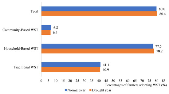
Figure 4.
Percentages of farmers adopting WSTs (%).
Table 3 presents crop yield per hectare and net crop income by the adopted WSTs. The Huang-Huai-Hai region is dominated by the rotation system of wheat and maize, and most farmers only grow these two crops in the year. Therefore, we only focused on farmers who grew wheat and maize, and crop yield and net crop income are also a sum of wheat and maize in this paper. The findings showed that, regardless of WST adoption, the average crop yield and net income per hectare in drought years are lower than those in normal years. For example, the average crop yield per hectare for plots with WSTs is 12,939 kg/ha in normal years and 11,835 kg/ha in drought years, and the average net income is 15,510 yuan/ha in normal years and 12,310 yuan/ha in drought years. Further, the crop yield per hectare and net crop income for the plots with WSTs are higher than for those plots without WSTs. For example, in drought years, for plots with WSTs, the crop yield per hectare and net crop income are 11,835 kg and 12,310 yuan per hectare, respectively, while, for plots without WSTs, the crop yield per hectare and net crop income are 9383 kg and 7260 yuan per hectare, respectively. The difference is about 2500 kg of crop and 5000 yuan per hectare. Further exploration is required to decide whether this gap is mainly caused by WST adoption or the heterogeneity of different plots.
Table 3.
Crop yield and net income by whether WST is adopted and drought year.
4. Model Specification and Test
4.1. The Endogenous Switching Regression
The combination of the decision model and the effect model raises the following problems. First, the decision to adopt WSTs is voluntary, which may lead to the problem of sample selection bias. Second, given that WST adoption is used as a decision variable to analyze its efficiency in relation to crop yield, yield risk, and net income of farmers, endogeneity problems may arise due to the omission of variables. Third, there is significant heterogeneity between adopters and non-adopters in terms of WSTs. Therefore, this paper uses the endogenous switching regression model (ESRM) to analyze the determinants of farmers’ WST adoption and their impact on crop yield, production risk, and the net income of farmers.
Specifically, the ESRM model is divided into two stages. In the first stage, the model uses a Probit regression to analyze and estimate the influencing factors of WST adoption; in the second stage, farmers are divided into two groups according to their different decisions (adopters and non-adopters in terms of WSTs), and the difference in effect between the two groups is estimated [45].
In the first stage, WSTi* is the latent variable of the dummy variable WSTi. The latent variable is specified as:
where farmland plot i is chosen for adaption by the farmer (WSTi = 1) to address drought. Xi is a vector of factors influencing WSTi adoption. Zi represents the instrument variable, and γ is the corresponding estimated parameter. The reason for selecting instrument variables is to ensure the model identifiability. It is required that at least one variable in the selection equation does not appear in the result equation, and this variable must satisfy the conditions that it affects farmers’ adoption decision but does not directly affect crop yield or net income. is a vector of parameters. is an error term where .
In the second stage, the outcome function can be defined as:
where Y1i and Y2i are the mean of crop yield, the risk of crop yield, and net crop income for adopters and non-adopters, respectively. X1i and X2i are a set of explanatory variables for adopters and non-adopters, respectively. β and are the corresponding estimated parameters.
Our analysis relies on a moment-based specification of the stochastic production function [46,47]. This method is widely used in agricultural economics to model the implication of weather risk and risk management [32,48]. This paper employs first-order moment and second-order moment estimation methods to represent the mean of crop yield and the variation of crop yield, respectively. The mean of crop yield is expressed as the expected value of yield, , and the variation of crop yield is expressed as the variance of yield, . Under the condition of production uncertainty, according to the first-order moment estimation method, the overall crop yield function can be defined as: , where indicates the expected value of overall crop yield. is a random error term representing the uncertainty of farmers facing drought, which satisfies . According to the definition of second-order center distance, crop yield variation can be expressed by the variance of crop yield: .
When unobservable factors affect both the choice variable WSTs and the result variable Y of adopters, the correlation coefficient of the error term in the choice equation and the result equation are not zero, that is, . In addition, since the expected values of the error terms and are not 0, direct estimation of the parameters (9) and (10) using OLS suffers from sample selection bias [43].
The three error terms , , and in Equations (8), (9), and (10) are assumed to have a trivariate normal distribution with mean vector zero and covariance matrix:
where , , , , , and . Due to the missing data (the results Y1i and Y2i of farmers in different adoption behaviors cannot be obtained at the same time), this paper introduces the inverse Mills ratio into the result equation to solve this problem [49]. The expected values of the error terms and of the resulting Equations (11) and (12) for the adopter and non-adopter are given as follows:
where the standard normal probability density function is , and is the normal cumulative distribution function. The terms and refer to the inverse Mills ratio evaluated at , respectively, and .
Here, this paper uses the full information maximum likelihood (FIML) method to estimate the ESRM, which advances the two-step least-squares and maximum likelihood methods [50]. Given the assumption of trivariate normal distribution for the error terms, the logarithmic likelihood function can be given as follows:
where , j = 1, 2, with denoting the correlation between the error term of the selection Equation (8) and the error term of Equations (11) and (12), respectively. is the correlation coefficient between and , and is the correlation coefficient between and . The estimated and are bounded between −1 and 1, and the estimated and are always positive. Additionally, full information maximum likelihood estimation for endogenous switching regression model can be achieved through the movestay command of STATA software [50].
4.2. Empirical Model
In order to examine the determinants of farmers adopting WSTs in response to drought, a specific selection model is established as follows:
In order to examine the effect difference of the WST measures, the separate outcome equations for adopters and non-adopters are defined as follows:
where the subscripts of i and h represent farmland plot and farmers, respectively. The subscript of c represents the county, and t represents the year. are the vectors of parameters to be estimated. , , and are the error terms. Table 4 presents the definition and descriptive statistics of variables used in the above equations.
Table 4.
Definitions and descriptive statistics of variables.
WSTiht is the dependent variable, which indicates that the percentage of farmers using WSTs reaches 80%, whether or not the hth household adopts WST measures at t year when the farm is on I plot. Yiht represents crop yield, crop production risk (yield variance), and net crop income, respectively. It can be seen from Table 4 that the average crop yield is 11,809 kg per hectare, the average crop variance is 0.38, and the net crop income for farmers is 12,760 yuan per hectare. Among them, the net income from grain growing is obtained by subtracting the actual input, which includes the cost of production factors such as fertilizers, pesticides, machinery, irrigation water, and labor costs from the total value of crop yield. This paper does not consider domestic labor discount in land costs and labor costs. The instrument variable is represented by the price of agricultural irrigation water Zct, and the average agricultural irrigation water is 1544 yuan per hectare.
Among the explanatory variables, Dct indicates whether a drought disaster t occurred at the county level. Factor input variables include fertilizer Iiht1, pesticide Iiht2, capital input for machinery Iiht3, and labor input Iiht4. Among them, the fertilizer input is the highest, at 4898 yuan per hectare. It is followed by the cost of mechanical operation (2561 yuan per hectare), the input of pesticides (821 yuan per hectare), and the labor input (92 labor days per hectare). Among the characteristic variables of farmers’ families, the average value of household durable goods Hht1 is 9610 yuan; the probability of family members having participated in agricultural production technique training Hht2 in the past three years is 25%; the gender indicator of household heads Hht3 is 0.95, indicating that 95% of household heads are males; the average education level Hht4 of the heads is 6.91 years, which is equivalent to the education level of junior high school; the average number of years of arable land Hht5 is 34.97 years. The characteristic variables of the plot include the arable land area of the plot Fiht1. The statistics showed that the average size of individual plot area is only 0.2 hectares, indicating that the arable land is fragmented and scattered; the land form of arable land Fiht2 is mainly flat land, with only 7% of farmers choosing to grow crops on the mountains. In terms of the property rights of land plot Fiht3, 95% of the land is owned by farmers, and only 5% is taken in loan from others; soil types include sandy soil Fiht41 (27%), loamy soil Fiht42 (35%), and clay soil Fiht43 (38%). In addition, the regional variable P is represented by five provinces, respectively.
4.3. Endogeneity and Instrument Variable Test
When WST adoption is used to explain crop yield or income, there may be endogeneity problems in farmers’ choice. Therefore, this study first needs to test whether the WST variable Siht is an endogenous explanatory variable. According to the Hausman test results, = 9.01 **, this study rejects the null hypothesis H0 that all explanatory variables are exogenous. According to the results of Durbin–Wu–Hausman test, Durbin (score) = 9.058 ***, Wu–Hausman F(1,3738) = 9.027 ***, it is further verified that WST variable WSTiht is an endogenous explanatory variable.
To this end, this study uses the agricultural irrigation water price Zct as an instrument variable of the WST variable WSTiht. First, an increase in water price can motivate or constrain farmers’ water-saving behavior and thus promote WST adoption. Second, considering changes in water prices are government actions, raising the price of irrigation water only affects farmers’ WST adoption, but does not directly affect the crop yields per hectare. Based on the above analysis and referring to the methods provided by Di Falco et al. [51] and Huang et al. [32], this study finds that the examination of the effect on the crop yield of all samples imposed by instrument variables is not enough to explain whether the change in yield is caused by instrument variables or by other water-saving measures. On the contrary, if only non-adopters are analyzed, it turns out that the change of water price has no effect on farmers’ adoption behavior, and does not affect the crop yield.
In Table 5, the Probit model set for the water-saving technology choices presents that the price of irrigation water plays a significant role in promoting the adoption of WSTs by farmers. The mixed-effects OLS model constructed for the crop yield per hectare shows that the price of irrigation water has no significant effect on crop yield. Therefore, it is valid to select the price of agricultural irrigation water as an instrument variable.
Table 5.
Endogenous test on instrument variables.
5. Estimated Results and Analyses
5.1. The Determinants of Adoption Decision
The estimated results for the determinants of farmers’ WST adoption are presented in column 2 of Table 6, Table 7 and Table 8. The instrument variable the price of agricultural irrigation water has a positive impact on WST adoption, indicating that the increase in the price promotes farmers’ WST adoption. The finding is consistent with previous studies on irrigation water price policy [52]. When water price is low, the water-saving enthusiasm of farmers is not reflected and nor is the scarcity of water resources. Raising water prices inevitably leads to increase input costs for farmers, and, thus, rational farmers invest in the more effective WST measures to minimize production costs. Therefore, water price increase can motivate or constrain farmers’ water-saving behavior and promote their WST adoption.
Table 6.
Farmers’ WST adoption decision and its impact on mean crop yield.
Table 7.
Farmers’ WST adoption decision and its impact on variance of crop yield.
One possible reason is that the adoption cost of the traditional WSTs and household-based WSTs is relatively low, and the adoption of WSTs is affected by farmers’ production behaviors and habits; thus, the potential coverage can be relatively wide. Due to the long-term trend of precipitation reduction in the surveyed area, farmers use the household-based WSTs regardless of whether they encounter drought or not. However, once a drought occurs, the adoption of community-based WSTs may be too late due to the high price, large amount of engineering, and long construction time.
In terms of production factor input, Table 6 shows that fertilizer input and mechanical input play a positive role in farmers’ adoption of WSTs. Specifically, when the fertilizer input increases by 10%, the possibility of farmers adopting WST increases by 3.08%, and when the mechanical input increases by 10%, the possibility of farmers adopting WSTs increases by 5.02%. It is apparent that the marginal effect of fertilizer input on the adoption of WSTs is larger than that of mechanical input. The possible explanations are: (i) theoretically, an increase from one factor input can possibly result in a change of factor input combination; (ii) increasing fertilizer input can cause crops to need more irrigation to obtain higher yield, which makes a larger possibility for farmers to adopt new WSTs; (iii) in fact, fertilizer and irrigation (or WSTs) are complementary from the perspective of crop nutrition.
In terms of the characteristic variable of farmers, family wealth has a positive effect on the WST adoption (Hht1 = 0.086, Table 7), indicating that relatively wealthy households are more likely to adopt WSTs to offset the crop loss caused by drought. Family member participation in production technology training and the education level of household heads also have a significant positive impact on the WST adoption. Specifically, when other conditions remain unchanged, if family members have received production technology training, the probability of adopting WST increases by 14.5%. For each additional education year of the household head, the probability of adopting WSTs increases by 2.2% (Table 7, row 17). Consistent with the research findings of scholars such as Zhang et al. [18], Mi et al. [26], and Yuan et al. [20], the present study finds that the higher the education level of farmers, the more willing they are to adopt WSTs. Farmers of higher education level demonstrate stronger ability to accept new technologies, and, thus, it is easier for them to seize opportunities.
Based on the above analysis, it may be concluded that a wide range of factors, including the price of agricultural irrigation water, farmers’ family wealth, production technology training, and education level of family members, significantly affects farm households’ WST adoption. Therefore, the government should speed up its efforts in establishing and implementing a reasonable agricultural water price system, properly raise the water price to strengthen farmers’ water-saving awareness, promote agricultural WSTs, and improve the efficiency of water resources utilization. In addition, the government should strengthen education and training in rural areas and find ways to increase farmers’ income.
5.2. Estimation of Mean Crop Yield Function
Table 6 shows the simultaneous results of the decision equation and the mean crop yield equation used in farmers’ WST adoption. The estimated results for factors affecting the crop yield of adopters and non-adopters are listed in columns 3 and 4, respectively.
First, the adoption of WSTs can reduce crop yield loss caused by drought. For example, for non-adopters, drought has a negative impact on mean crop yield (−0.011), while for adopters, drought has a positive effect on mean crop yield (0.069), which suggests that the adoption of WSTs mitigates the loss of crop production caused by drought.
Second, the input of production factors can significantly affect the mean crop yield per unit area. Fertilizers, pesticides, machinery, and labor all have significantly positive effects on crop yield per unit area; however, their coefficients are all less than 1, indicating that the inputs of all factors are inelastic.
Third, among the household characteristics, the education level of the household heads has a significant role in promoting the mean crop yield per unit area. For example, for non-adaptors, each additional education year of the heads increases the crop yield per unit area by 2.4%.
Fourth, among the plot characteristics, land area has a significantly positive effect on the mean crop yield per unit area. In this regard, the larger the scale of crop growing, the higher the level of crop yield, that is, the scale of land management can guarantee crop yield.
5.3. Estimation of Crop Risk Function
The regression results of the impact of WSTs on variance of crop yield are shown in Table 7. The estimated results for adopters and non-adopters are listed in columns 3 and 4, respectively. From the overall results, the estimated values of the correlation coefficients and of the error terms between the selection equation and the result equation pass the 1% significance level, indicating that there is sample selection bias. In addition, and have the same sign, which means that the WST adoption by crop household is based on hierarchical ranking. The key findings are as follows.
First, the estimated coefficient in the variance function of non-adopters is 0.083, which is higher than that of the adopters (0.001) with the drought. Although the coefficient is not significant, it shows that the adoption of WSTs can reduce crop yield variation to a certain degree.
Second, the production factor input can significantly reduce the risk of crop yield. Table 7 shows that the costs of chemical fertilizers, pesticides, machinery, and labor all have a significantly negative impact on the variance of crop yield.
Third, household characteristics such as family wealth, the education of household heads, and the farming experience also significantly affect the risk of crop yield. For example, for adopters, every 1% increase in the value of household’s durable goods reduces the variance of crop yield by 0.028%. For each additional year of farming experience, the variance of crop yield decreases by 0.1%.
5.4. Estimation of Crop Income Function
Table 8 shows the simultaneous results for farmers’ WST selection equation and net crop income equation. The factors affecting farmers’ adoption of WSTs are consistent with the above results and, thus, are not repeated here. According to the estimation results of the impact on net crop income, the elasticity and sign of factor input have obvious differences in their impact on crop yield. Specifically, fertilizer and pesticide have a significantly positive effect on crop yield, while the effects of fertilizer and pesticide on net crop income are not significant but negative. Possible reasons are the high cost of inputs or the low return from increased production [35]. In detail, the marginal net income cannot offset the marginal input cost. The possible reason is that gain price is relatively low compared to the fertilizer price. Therefore, the government encourages farmers to reduce fertilizer use.
Table 8.
Farmers’ WST adoption decision and its impact on net crop income.
Table 8.
Farmers’ WST adoption decision and its impact on net crop income.
| Variables | WST Adoption Decision | Net Crop Income (log) | |
|---|---|---|---|
| Adopters | Non-Adopters | ||
| If it is drought year Dct | −0.023 | −0.106 *** | −0.057 *** |
| (0.054) | (0.006) | (0.017) | |
| Fertilizer cost log Iiht1 | 0.139 | −0.016 | 0.046 *** |
| (0.093) | (0.017) | (0.017) | |
| Pesticide cost log Iiht2 | 0.000 | −0.005 | −0.002 |
| (0.070) | (0.009) | (0.012) | |
| Machinery cost log Iiht3 | 0.334 *** | 0.036 * | −0.024 |
| (0.079) | (0.022) | (0.015) | |
| Labor cost log Iiht4 | 0.058 | 0.027 ** | −0.018 |
| (0.088) | (0.011) | (0.021) | |
| Durable goods of family log Hht1 | 0.114 ** | 0.011 * | 0.001 |
| (0.054) | (0.007) | (0.022) | |
| If family members have received agricultural production technology training in the past 3 years Hht2 | 0.065 | 0.013 | 0.028 |
| (0.121) | (0.015) | (0.035) | |
| Gender of HH head Hht3 | 0.036 | 0.016 | −0.196 ** |
| (0.214) | (0.032) | (0.092) | |
| Education of HH head Hht4 | 0.034 ** | 0.004 * | 0.020 *** |
| (0.017) | (0.002) | (0.007) | |
| Farming experience of head Hht5 | −0.001 | 0.002 ** | 0.001 |
| (0.005) | (0.001) | (0.002) | |
| Farmland area Fiht1 | −0.025 | 0.135 *** | 0.111 *** |
| (0.295) | (0.033) | (0.042) | |
| Farmland types Fiht2 | 0.999 *** | −0.008 | 0.029 |
| (0.243) | (0.031) | (0.048) | |
| Farmland property Fiht3 | 0.163 | 0.022 | −0.045 |
| (0.207) | (0.023) | (0.040) | |
| If soil is loam or not Fiht42 | 0.068 | 0.053 *** | 0.081 |
| (0.169) | (0.017) | (0.057) | |
| If soil is clay or not Fiht43 | 0.017 | 0.053 *** | 0.073 |
| (0.175) | (0.017) | (0.065) | |
| Price of agricultural irrigation water Zct | 0.495 *** | - | - |
| (0.056) | - | - | |
| Province dummies P | YES | YES | YES |
| Constant | −4.034 *** | 3.120 *** | 2.946 *** |
| (0.695) | (0.266) | (0.369) | |
| - | 0.209 *** | 0.276 ** | |
| - | (0.055) | (0.121) | |
| - | 0.165 | −0.525 | |
| - | (0.125) | (0.515) | |
| Obs. (plots) | 3760 | 3015 | 745 |
Notes: Robust standard errors are in parentheses. *, **, and *** represent significance at the 10%, 5%, and 1% level, respectively.
5.5. Effects of WSTs on Crop Yield, Risk, and Net Income
Table 9 presents the expected results and average treatment effects of WST selection decisions on variances of crop yield and net crop income. Notes (a) and (b) reflect the true expected values of crop yield, yield risk, and net crop income, while notes (c) and (d) reflect the counterfactual results of the three.
Table 9.
Average treatment effects of WST adopters.
The estimation results for ATT show that the adoption of WSTs significantly decreases crop yield loss and net income loss. Specifically, compared with the counterfactual case where farmers do not adopt WSTs, farmers who adopt decrease the loss of mean crop yield and net crop income by 14.92% and 13.45% per hectare, respectively. Furthermore, the adoption of WSTs reduces crop yield variation by 11.61% per hectare. The estimation results for ATU reveal that if non-adopters have the opportunity to adopt WSTs, their crop yield and net crop income decrease the loss of mean crop yield and net crop income by 3.50% and 2.32%, respectively, and crop yield variation can be reduced by 7.23%.
In Table 10, the plots are classified according to the adoption situations of different WST measures and then the treatment effects of traditional WSTs, household-based WSTs, and community-based WSTs are calculated. Compared with the counterfactual results, the crop yield per unit area increases by 10.22% for traditional WST adopters, 14.09% for household-based WST adopters, and 14% for community-based WST adopters. Compared with the counterfactual results, the net crop income increases by 4.59%, 12.18%, and 14.52%, respectively, for the HHs which adopt the traditional WSTs, household-based WSTs, and community-based WSTs. The above results show that no matter what kind of WST farmers adopt, their crop yield and the net crop income are significantly improved. Furthermore, compared with traditional WST adopters, there is a large increase in crop yield and net income for household-based WST adopters and community-based WST adopters.
Table 10.
Average treatment effects of farmers adopting different types of WST.
The mixed-effects model (POOL-OLS) that explains the effects of different WSTs on crop yield and net income also gives similar results (Table 11). The adoption of traditional WSTs has no significant impact on crop yield per unit area, while the adoption of household-based WSTs and community-based WSTs has a significant effect. Specifically, when other conditions remain unchanged, the adoption of household-based WSTs and community-based WSTs can increase the crop yield by 8.5% and 6.6%, respectively. As to the net crop income, the adoption of the traditional WSTs can increase the net crop income by 10.7%, and the adoption of the household-based WSTs and community-based WSTs can greatly increase it, by 16.6% and 14.3%, respectively.
Table 11.
The effect of different WST on crop yield and net crop income per hectare (POOL-OLS).
6. Conclusions and Discussion
This paper constructed a decision-making model and an effect model based on expected utility maximization to study how farm households cope with drought by adopting WSTs. Using the micro field survey data of farm households in five provinces across the Huang-Huai-Hai region, endogenous switching regression was used to identify the influencing factors of farm households’ adoption of WSTs and its impact on crop yield, yield variation, and net crop income. Further, the treatment effects of traditional WSTs, household-based WSTs, and community-based WSTs were analyzed.
6.1. Conclusions
First, the adoption of WSTs significantly reduces crop yield loss caused by drought. In detail, adopting WSTs significantly decreases crop yield loss and net crop income loss by 14.92% and 13.45%, respectively. Meanwhile, adopting WSTs reduces crop yield variation by 11.61% per hectare. Therefore, in the context of the increasing frequency of drought in the Huang-Huai-Hai region, WSTs effectively cope with drought and ensure crop production.
Second, WSTs are different in terms of adoption frequency and drought resistance effects. Traditional WSTs and household-based WSTs are much more frequently adopted than community-based WSTs. This result might be due to the fact that traditional WSTs and household-based WSTs have lower investment costs and are easier to popularize than community-based WSTs. In addition, community-based WSTs may need more group cooperation.
Third, various WSTs can be adopted to suit different household production functions. Compared with traditional WSTs, for example, adopting household-based and community-based WST can be more effective for saving crop yield and net crop income.
Finally, raising the price of irrigation can play a significant role in promoting the adoption of WSTs by farmers. This finding indicates that water price can encourage farm households to improve water use efficiency by adopting WSTs.
6.2. Discussion
In dialogue with the existing literature, we responded to and confirmed the scholarly view that the WSTs can help farmers to effectively cope with drought and save crop production. Therefore, application of WSTs is certainly important for this major, irrigated crop-planting area in China.
First, increasing fertilizer input can increase the possibility of adopting WSTs. This finding is more feasible for yield-induced farmers. Therefore, currently, land circulation and scale management may be one of the priorities for Chinese crop production sector.
Second, agricultural irrigation is closely correlated with land consolidation. The application of WSTs can increase crop production cost, which may make it infeasible for farmers to adopt more advanced WSTs. The preparation of high-standard farmland can be another capital construction project for China’s future agriculture.
Third, institutional reform is also important for the adoption of WSTs by farm households. For example, raising the water price can make farmers more likely to adopt WSTs. Similarly, increasing machinery input can also make farmers likely to adopt WSTs, and, therefore, increasing agricultural machinery subsidies could be another policy option. Therefore, it would be useful for the government to conduct some agricultural institutional reforms.
As usual, this study still has some limitations. Our classification of WSTs was very general and did not consider the types of technologies in detail. For example, the adaptation measures did not take into consideration the adjusting of crop varieties and the use of drought-resistant varieties. In addition, the data need to be updated, and the results should be used with caution.
Author Contributions
Conceptualization, C.S. and H.M.; methodology, C.S.; software, Y.R.; validation, R.L. and L.O.; formal analysis, R.L.; investigation, C.S. and Y.R.; resources, Y.R.; data curation, C.S.; writing—original draft preparation, C.S. and Y.R.; writing—review and editing, L.O. and H.M.; visualization, R.L.; supervision, L.O. and H.M.; project administration, C.S. and H.M.; funding acquisition, C.S. and Y.R. All authors have read and agreed to the published version of the manuscript.
Funding
This research was funded by the National Natural Science Foundation of China (Grant No. 72003057; 72173037), Ministry of Education of Humanities and Social Science Research Project of China (Grant No. 21YJA790039), Henan Province Philosophy and Social Science Planning Project (Grant No. 2021BJJ046; 2022CJJ147), Key Scientific Research Project of Henan Provincial Institutions of Higher Learning (Grant No. 21A790011), Research Project of Henan Social Science Federation (Grant No. SKL-2022-2221).
Data Availability Statement
The data are available on request from the corresponding author.
Conflicts of Interest
There is no conflict of interest.
References
- Rosa, L.; Chiarelli, D.D.; Rulli, M.C.; Dell’Angelo, J.; Odorico, P. Global agricultural economic water scarcity. Sci. Adv. 2020, 6, 6031–6060. [Google Scholar] [CrossRef] [PubMed]
- Intergovernmental Panel on Climate Change (IPCC). Managing the Risks of Extreme Events and Disasters to Advance Climate Change Adaptation. Special Report of the Intergovernmental Panel on Climate Change; Cambridge University Press: Cambridge, UK, 2020. [Google Scholar]
- Fitton, N.; Alexander, P.; Arnell, N.; Bajzelj, B.; Calvin, K.; Doelman, J.; Gerber, J.S.; Havlik, P.; Hasegawa, T.; Herrero, M.; et al. The vulnerabilities of agricultural land and food production to future water scarcity. Glob. Environ. Chang. 2019, 58, 101944. [Google Scholar] [CrossRef]
- Cao, X.; Wu, M.; Guo, X.; Wu, N.; Wang, W. Assessing water scarcity in agricultural production system based on the generalized water resources and water footprint framework. Sci. Total Environ. 2017, 609, 587–597. [Google Scholar]
- Zhou, S.; Herzfeld, T.; Glauben, T.; Zhang, Y.; Hu, B. Factors affecting Chinese farmers’ decisions to adopt a water-saving technology. Can. J. Agric. Econ. 2008, 56, 51–61. [Google Scholar] [CrossRef]
- Wang, S.; Yin, N.; Yang, Z. Factors affecting sustained adoption of irrigation water-saving technologies in groundwater over-exploited areas in the North China Plain. Environ. Dev. Sustain. 2021, 23, 10528–10546. [Google Scholar] [CrossRef]
- Wang, J.; Yang, Y.; Huang, J.; Adhikari, B. Adaptive irrigation measures in response to extreme weather events: Empirical evidence from the North China plain. Reg. Environ. Chang. 2019, 19, 1009–1022. [Google Scholar] [CrossRef]
- National Bureau of Statistics. China Statistics Yearbook; China Statistics Press: Beijing, China, 2020. (In Chinese)
- Ministry of Water Resources of, P.R. China. China Flood and Drought Disaster Prevention Bulletin; China Water Conservancy Press: Beijing, China, 2020. (In Chinese) [Google Scholar]
- Saini, M.; Dutta, V.; Joshi, P.K. Reassessment of drought management policies for India: Learning from Israel, Australia, and China. Environ. Sustain. 2021, 4, 671–689. [Google Scholar] [CrossRef]
- Belder, P.; Bouman, B.; Cabangon, R.; Lu, G.; Quilang, E.; Li, Y.; Spiertz, J.H.J.; Tuong, T.P. Effect of water-saving irrigation on rice yield and water use in typical lowland conditions in Asia. Agric. Water Manag. 2004, 65, 193–210. [Google Scholar] [CrossRef]
- Huang, Q.; Wang, J.; Li, Y. Do water saving technologies save water? Empirical evidence from North China. J. Environ. Econ. Manag. 2017, 82, 1–16. [Google Scholar] [CrossRef]
- Vatta, K.; Sidhu, R.; Lall, U.; Birthal, P.; Taneja, G.; Kaur, B.; Devineni, N.; MacAlister, C. Assessing the economic impact of a low-cost water-saving irrigation technology in Indian Punjab: The tensiometer. Water Int. 2018, 43, 305–321. [Google Scholar] [CrossRef]
- Li, J.; Wang, Y.; Zhang, M.; Liu, Y.; Xu, X.; Lin, G.; Wang, Z.; Yang, Y.; Zhang, Y. Optimized micro-sprinkling irrigation scheduling improves grain yield by increasing the uptake and utilization of water and nitrogen during grain filling in winter wheat. Agric. Water Manag. 2019, 211, 59–69. [Google Scholar] [CrossRef]
- Zhai, L.; Lv, L.; Dong, Z.; Zhang, L.; Zhang, J.; Jia, X.; Zhang, Z. The water-saving potential of using micro-sprinkling irrigation for winter wheat production on the North China Plain. J. Integr. Agric. 2021, 20, 1687–1700. [Google Scholar] [CrossRef]
- Guo, E.; Yang, X.; Li, T.; Zhang, T.; Yang, Y. Does ENSO strongly affect rice yield and water application in Northeast China. Agric. Water Manag. 2021, 245, 106605. [Google Scholar] [CrossRef]
- National Bureau of Statistics. China Statistics Yearbook; China Statistics Press: Beijing, China, 2021. (In Chinese)
- Zhang, B.; Fu, Z.; Wang, J.; Zhang, L. Farmers’ adoption of water-saving irrigation technology alleviates water scarcity in metropolis suburbs: A case study of Beijing, China. Agric. Water Manag. 2019, 212, 349–357. [Google Scholar] [CrossRef]
- Liu, M.; Yang, L.; Bai, Y.; Min, Q. The impacts of farmers’ livelihood endowments on their participation in eco-compensation policies: Globally important agricultural heritage systems case studies from China. Land Use Policy 2018, 77, 231–239. [Google Scholar] [CrossRef]
- Yuan, K.; Yang, Z.; Wang, S. Water scarcity and adoption of water-saving irrigation technologies in groundwater over-exploited areas in the North China Plain. Irrig. Sci. 2021, 39, 397–408. [Google Scholar] [CrossRef]
- Ma, J.; Cui, Y.; Kong, X.; Chen, Z. Water rights system, water drawing permission and farmers’ adoption of water-saving technology: An empirical study on water-saving effects of water rights reforms based on the difference approach. Stat. Res. 2021, 38, 116–130. (In Chinese) [Google Scholar]
- Blanke, A.; Rozelle, S.; Lohmar, B.; Wang, J.; Huang, J. Water saving technology and saving water in China. Agric. Water Manag. 2007, 87, 139–150. [Google Scholar] [CrossRef]
- Zou, X.X.; Li, Y.; Cremades, R.; Gao, Q.Z.; Wan, Y.F.; Qin, X.B. Cost-effectiveness analysis of water-saving irrigation technologies based on climate change response: A case study of China. Agric. Water Manag. 2013, 129, 9–20. [Google Scholar] [CrossRef]
- Alauddin, M.; Sarker, M.R.; Islam, Z.; Tisdell, C. Adoption of alternate wetting and drying (AWD) irrigation as a water-saving technology in Bangladesh: Economic and environmental considerations. Land Use Policy 2020, 91, 104430. [Google Scholar] [CrossRef]
- Jara-Rojas, R.; Bravo-Ureta, B.E.; Díaz, J. Adoption of water conservation practices: A socioeconomic analysis of small-scale farmers in central Chile. Agric. Syst. 2012, 110, 54–62. [Google Scholar] [CrossRef]
- Mi, Q.; Li, X.; Li, X.; Yu, G.; Gao, J. Cotton farmers’ adaptation to arid climates: Waiting times to adopt water-saving technology. Agric. Water Manag. 2021, 244, 106596. [Google Scholar] [CrossRef]
- Person, M.T.; Delea, M.G.; Garn, J.V.; Alexander, K.; Abaire, B.; Freeman, M.C. Assessing the influence of social capital on water point sustainability in rural Ethiopia. J. Water Sanit. Hyg. Dev. 2017, 7, 611–622. [Google Scholar] [CrossRef]
- Sharma, A.; Bharti, A.; Saha, A.; Sharma, J.; Jamwa, S. Influence of various water saving techniques on yield and water productivity of irrigated rice: A review. Int. J. Curr. Microbiol. Appl. Sci. 2021, 10, 1993–2004. [Google Scholar] [CrossRef]
- Chen, Z.; Li, P.; Jiang, S.; Chen, H.; Cao, C. Evaluation of resource and energy utilization, environmental and economic benefits of rice water-saving irrigation technologies in a rice-wheat rotation system. Sci. Total Environ. 2021, 757, 143748. [Google Scholar] [CrossRef]
- Wang, H.; Zhang, Y.; Zhang, Y.; McDaniel, M.; Sun, L.; Su, W.; Fan, X.; Liu, S.; Xiao, X. Water-saving irrigation is a ‘win-win’ management strategy in rice paddies–With both reduced greenhouse gas emissions and enhanced water use efficiency. Agric. Water Manag. 2020, 228, 105889. [Google Scholar] [CrossRef]
- Zhuang, Y.; Zhang, L.; Li, S.; Liu, H.; Zhai, L.; Zhou, F.; Ye, Y.; Ruan, S.; Wen, W. Effects and potential of water-saving irrigation for rice production in China. Agric. Water Manag. 2019, 217, 374–382. [Google Scholar] [CrossRef]
- Huang, J.; Wang, Y.; Wang, J. Farmers’ adaptation to extreme weather events through farm management and its impacts on the mean and risk of rice yield in China. Am. J. Agric. Econ. 2015, 97, 602–617. [Google Scholar] [CrossRef]
- Khanal, U.; Wilson, C.; Lee, B.; Hoang, V. Climate change adaptation strategies and food productivity in Nepal: A counterfactual analysis. Clim. Chang. 2018, 148, 575–590. [Google Scholar] [CrossRef]
- Ojo, T.O.; Baiyegunhi, L.J.S. Determinants of climate change adaptation strategies and its impact on the net farm income of rice farmers in south-west Nigeria. Land Use Policy 2020, 95, 03946. [Google Scholar] [CrossRef]
- Song, C.; Liu, R.; Oxley, L.; Ma, H. The adoption and impact of engineering-type measures to address climate change: Evidence from the major grain-producing areas in China. Aust. J. Agric. Resour. Econ. 2018, 62, 608–635. [Google Scholar] [CrossRef]
- Wang, Y.; Huang, J.; Wang, J.; Findlay, C. Mitigating rice production risks from drought through improving irrigation infrastructure and management in China. Aust. J. Agric. Resour. Econ. 2018, 62, 161–176. [Google Scholar] [CrossRef]
- Zhang, T.; Wang, J.; Teng, Y. Adaptive effectiveness of irrigated area expansion in mitigating the impacts of climate change on crop yields in northern China. Sustainability 2017, 9, 851–864. [Google Scholar] [CrossRef]
- Singh, I.; Squire, L.; Strauss, J. Agricultural Household Models: Extensions, Applications and Policy; Johns Hopkins University Press: Baltimore, MD, USA, 1986. [Google Scholar]
- Hazell, P. Application of risk preference estimates in firm-household and agricultural sector models. Am. J. Agric. Econ. 1982, 64, 384–390. [Google Scholar] [CrossRef]
- Riesgo, L.; Gomez-Limon, J.A. Multi-criteria policy scenario analysis for public regulation of irrigated agriculture. Agric. Syst. 2006, 91, 1–28. [Google Scholar] [CrossRef]
- Wallenius, J.; Dyer, J.S.; Fishburn, P.C.; Steuer, R.E.; Zionts, S.; Deb, K. Multiple criteria decision making, multiattribute utility theory: Recent accomplishments and what lies ahead. Manag. Sci. 2008, 54, 336–1349. [Google Scholar] [CrossRef]
- Liu, Y.; Huang, J. A Multi-objective Decision Model of Farmers’ Crop Production. Econ. Res. J. 2010, 45, 148–157. (In Chinese) [Google Scholar]
- Just, R.E.; Pope, R.D. Production Function Estimation and Related Risk Considerations. Am. J. Agric. Econ. 1979, 61, 276–284. [Google Scholar] [CrossRef]
- China Meteorological Administration (CMA). Trial Procedures for the Early-Warning Signal Issuance of Unexpected Meteorological Disasters; China Meteorological Administration: Beijing, China, 2004. (In Chinese)
- Lee, L.F. Unionism and wage rates: A simultaneous equations model with qualitative and limited dependent variables. Int. Econ. Rev. 1978, 19, 415–433. [Google Scholar] [CrossRef]
- Antle, J.M. Testing the stochastic structure of production: A flexible moment-based approach. J. Bus. Econ. Stat. 1983, 1, 192–201. [Google Scholar]
- Antle, J.M.; Goodger, W.M. Measuring stochastic technology: The case of Tulare milk production. Am. J. Agric. Econ. 1984, 66, 342–350. [Google Scholar] [CrossRef]
- Di Falco, S.; Chavas, J.P. On Crop Biodiversity, risk exposure and Food Security in the Highlands of Ethiopia. Am. J. Agric. Econ. 2009, 91, 599–611. [Google Scholar] [CrossRef]
- Greene, W.H. Econometric Analysis; Prentice Hall: Hoboken, NJ, USA, 2003. [Google Scholar]
- Lokshin, M.; Sajaia, Z. Maximum likelihood estimation of endogenous switching regression models. Stata J. 2004, 4, 282–289. [Google Scholar] [CrossRef]
- Di Falco, S.; Veronesi, M.; Yesuf, M. Does adaptation to climate change provide food security? A micro-perspective from Ethiopia. Am. J. Agric. Econ. 2011, 93, 829–846. [Google Scholar] [CrossRef]
- Xu, L.; Wang, N. Influence of agricultural water price on water saving behavior of farmers with different planting scales. J. Arid Land Resour. Environ. 2021, 35, 81–88. (In Chinese) [Google Scholar]
Publisher’s Note: MDPI stays neutral with regard to jurisdictional claims in published maps and institutional affiliations. |
© 2022 by the authors. Licensee MDPI, Basel, Switzerland. This article is an open access article distributed under the terms and conditions of the Creative Commons Attribution (CC BY) license (https://creativecommons.org/licenses/by/4.0/).