
Land Consumption Mapping with Convolutional Neural Network: Case Study in Italy


Abstract
:1. Introduction
1.1. Background
1.2. Operational Requirements
1.3. Objective
- Testing of the DL in consumed land mapping;
- Automatic production of thematic maps with the aim of improving accuracy and reducing costs and time compared with traditional techniques;
- Demonstration of the strategic importance of artificial intelligence for the future of environmental monitoring, with particular reference to land consumption mapping.
2. Materials and Methods
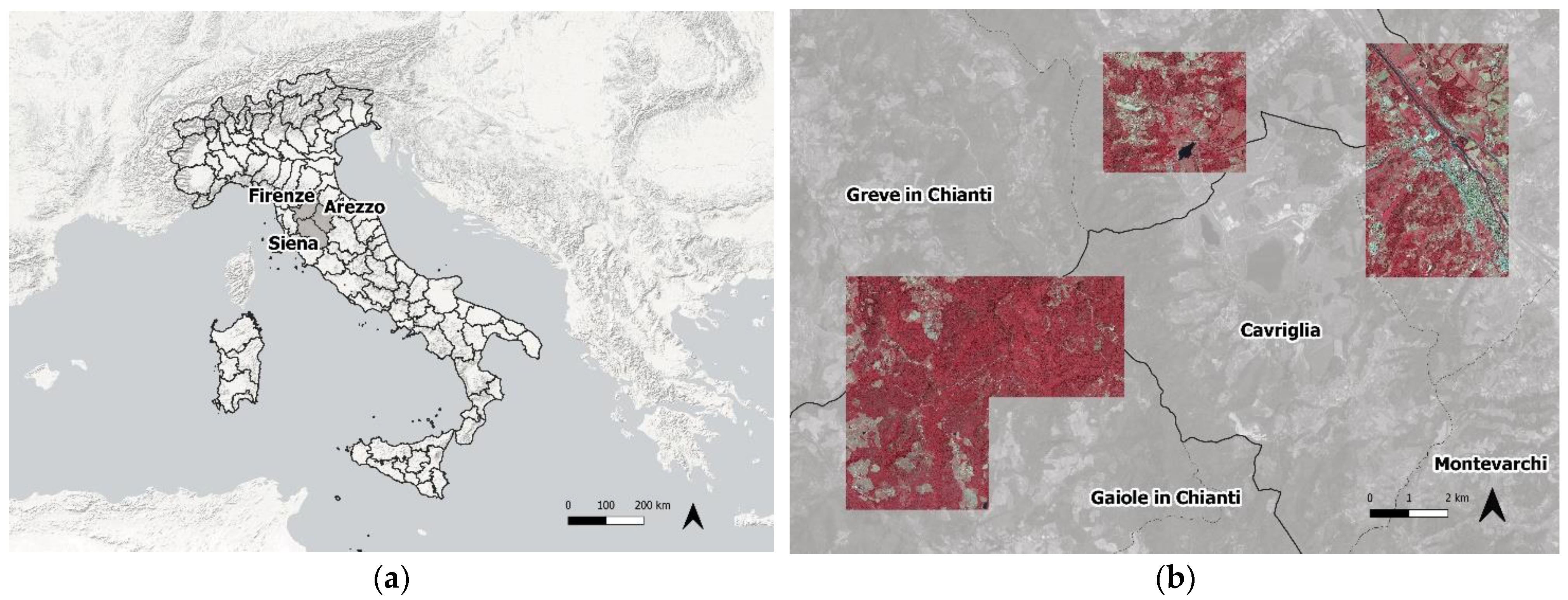
2.1. Study Area
2.2. Overview
- Scenario 1—binary classification distinguishing buildings from the residual areas;
- Scenario 2—binary classification distinguishing consumed land and non-consumed land;
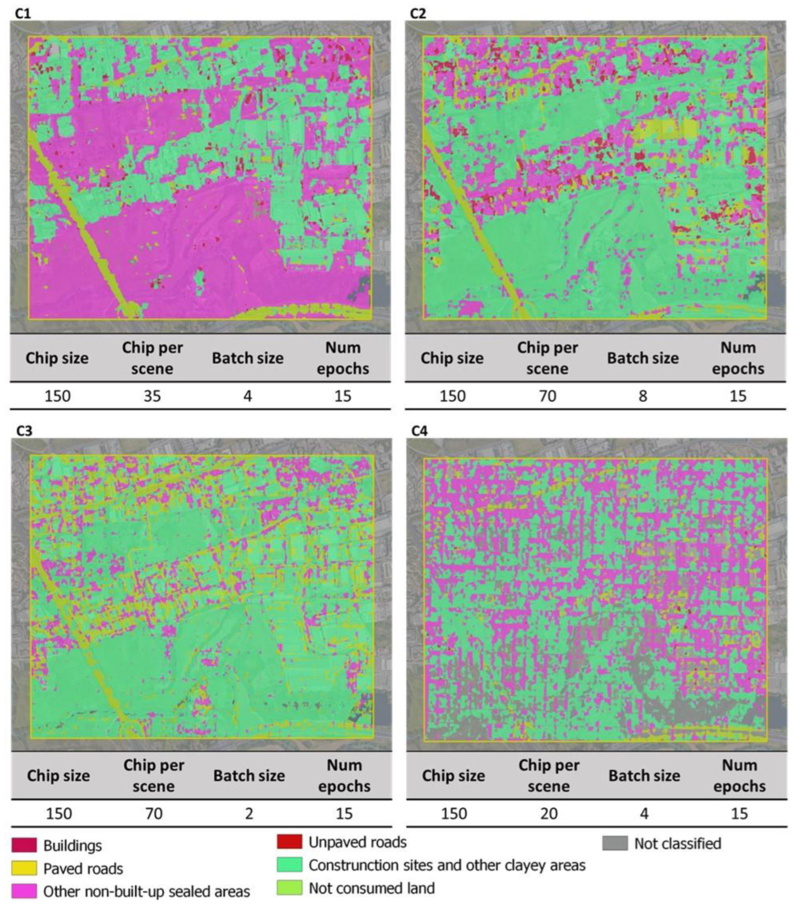
- Scenario 3—identification and distinction of different consumed land classes from natural areas.
2.3. Data Pre-Processing and Modeling
2.3.1. Pre-Processing
- The AGEA orthophotos (in raster format) were reprojected in the UTM WGS84 reference system and resampled to obtain square pixels. The spectral resolution was reduced to 3 bands: the blue region (500–520 nm) was removed since it is the least significant for artificial surfaces classification, although it led to a reduction in the information content. The radiometric resolution was also reduced: the 16 bit orthophotos were converted into 8 bit ones.
- The LCM was reprojected in the UTM WGS84 reference system, subjected to topological verification, and converted to Geojson format. The map has a three-level classification system, which distinguishes different consumed land classes. The data was reclassified to be suitable for the analysis of the three scenarios (Table 1).
2.3.2. Deep Residual Networks
2.3.3. Modeling
2.4. Deployment and Accuracy Assessment
3. Results
3.1. Modeling
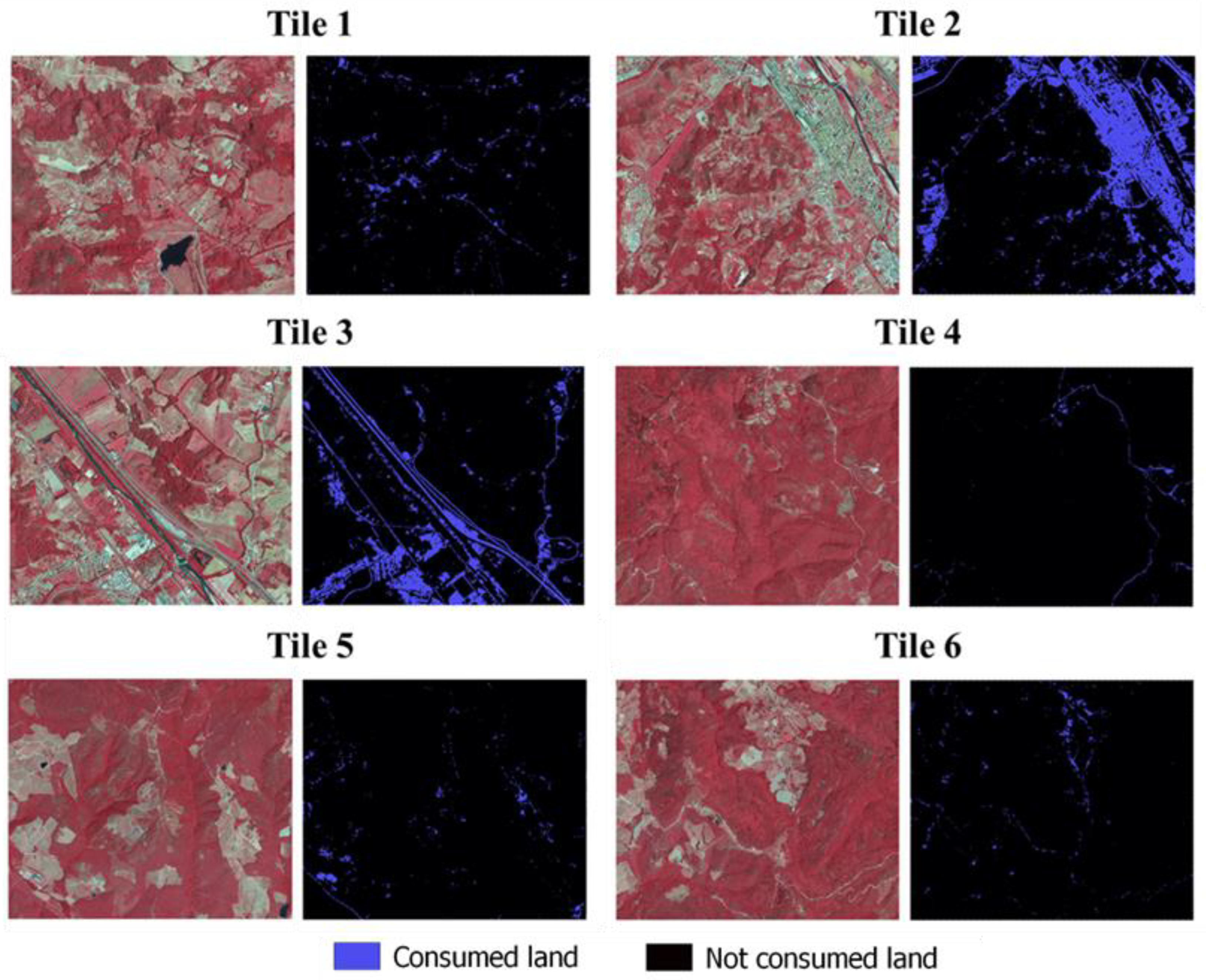
3.2. Deployment
- First, a visual comparison with orthophotos;
- Then, calculating the accuracy with the SCP plug-in by comparing predictions with the binary version of the LCM (1 = consumed land, 0 = non-consumed land) (Table 3).
4. Discussion
5. Conclusions
Author Contributions
Funding
Institutional Review Board Statement
Informed Consent Statement
Data Availability Statement
Conflicts of Interest
References
- De Fioravante, P.; Luti, T.; Cavalli, A.; Giuliani, C.; Dichicco, P.; Marchetti, M.; Chirici, G.; Congedo, L.; Munafò, M. Multispectral Sentinel-2 and Sar Sentinel-1 Integration for Automatic Land Cover Classification. Land 2021, 10, 611. [Google Scholar] [CrossRef]
- Munafò, M. Consumo Di Suolo, Dinamiche Territoriali e Servizi Ecosistemici; Edizione 2021; ISPRA, SNPA: Rome, Italy, 2021; ISBN 9788844810597. [Google Scholar]
- Chirici, G.; Giannetti, F.; Mazza, E.; Francini, S.; Travaglini, D.; Pegna, R.; White, J.C. Monitoring Clearcutting and Subsequent Rapid Recovery in Mediterranean Coppice Forests with Landsat Time Series. Ann. For. Sci. 2020, 77, 1–14. [Google Scholar] [CrossRef]
- Marchetti, M.; Vizzarri, M.; Sallustio, L. Towards Countryside Revival: Reducing Impacts of Urban Expansion on Land Benefits. In Agrourbanism; Springer: Berlin/Heidelberg, Germany, 2019; pp. 207–222. [Google Scholar]
- Costanza, R.; d’Arge, R.; de Groot, R.; Farber, S.; Grasso, M.; Hannon, B.; Limburg, K.; Naeem, S.; O’neill, R.V.; Paruelo, J. The Value of the World’s Ecosystem Services and Natural Capital. Nature 1997, 387, 253–260. [Google Scholar] [CrossRef]
- Strollo, A.; Smiraglia, D.; Bruno, R.; Assennato, F.; Congedo, L.; de Fioravante, P.; Giuliani, C.; Marinosci, I.; Riitano, N.; Munafò, M. Land Consumption in Italy. J. Maps 2020, 16, 113–123. [Google Scholar] [CrossRef]
- Shukla, P.R.; Skeg, J.; Buendia, E.C.; Masson-Delmotte, V.; Pörtner, H.-O.; Roberts, D.C.; Zhai, P.; Slade, R.; Connors, S.; van Diemen, S. Climate Change and Land: An IPCC Special Report on Climate Change, Desertification, Land Degradation, Sustainable Land Management, Food Security, and Greenhouse Gas Fluxes in Terrestrial Ecosystems; Intergovernmental Panel on Climate Change: Geneva, Switzerland, 2019.
- Dewan, A.M.; Yamaguchi, Y. Land Use and Land Cover Change in Greater Dhaka, Bangladesh: Using Remote Sensing to Promote Sustainable Urbanization. Appl. Geogr. 2009, 29, 390–401. [Google Scholar] [CrossRef]
- Lal, R. Restoring Soil Quality to Mitigate Soil Degradation. Sustainability 2015, 7, 5875–5895. [Google Scholar] [CrossRef] [Green Version]
- Oldeman, L.R.; Hakkeling, R.T.A.; Sombroek, W.G. World Map of the Status of Human-Induced Soil Degradation: An Explanatory Note; International Soil Reference and Information Centre: Wageningen, The Netherlands, 1990; ISBN 9066720425. [Google Scholar]
- Cowie, A.L.; Orr, B.J.; Castillo Sanchez, V.M.; Chasek, P.; Crossman, N.D.; Erlewein, A.; Louwagie, G.; Maron, M.; Metternicht, G.I.; Minelli, S.; et al. Land in Balance: The Scientific Conceptual Framework for Land Degradation Neutrality. Environ. Sci. Policy 2018, 79, 25–35. [Google Scholar] [CrossRef]
- Attri, P.; Chaudhry, S.; Sharma, S. Remote Sensing & GIS Based Approaches for LULC Change Detection—A Review. Int. J. Curr. Eng. Technol. 2015, 5, 3126–3137. [Google Scholar]
- Shalaby, A.; Tateishi, R. Remote Sensing and GIS for Mapping and Monitoring Land Cover and Land-Use Changes in the Northwestern Coastal Zone of Egypt. Appl. Geogr. 2007, 27, 28–41. [Google Scholar] [CrossRef]
- Rogan, J.; Chen, D.M. Remote Sensing Technology for Mapping and Monitoring Land-Cover and Land-Use Change. Prog. Plan. 2004, 61, 301–325. [Google Scholar] [CrossRef]
- Winkler, K.; Fuchs, R.; Rounsevell, M.; Herold, M. Global Land Use Changes Are Four Times Greater than Previously Estimated. Nat. Commun. 2021, 12, 2501. [Google Scholar] [CrossRef] [PubMed]
- Solórzano, J.V.; Mas, J.F.; Gao, Y.; Gallardo-Cruz, J.A. Land Use Land Cover Classification with U-Net: Advantages of Combining Sentinel-1 and Sentinel-2 Imagery. Remote Sens. 2021, 13, 3600. [Google Scholar] [CrossRef]
- Luti, T.; de Fioravante, P.; Marinosci, I.; Strollo, A.; Riitano, N.; Falanga, V.; Mariani, L.; Congedo, L.; Munafò, M. Land Consumption Monitoring with Sar Data and Multispectral Indices. Remote Sens. 2021, 13, 1586. [Google Scholar] [CrossRef]
- Munafò, M. Consumo Di Suolo, Dinamiche Territoriali e Servizi Ecosistemici; ISPRA, SNPA: Rome, Italy, 2019. [Google Scholar]
- Gandomi, A.; Haider, M. Beyond the Hype: Big Data Concepts, Methods, and Analytics. Int. J. Inf. Manag. 2015, 35, 137–144. [Google Scholar] [CrossRef] [Green Version]
- Audebert, N.; Saux, B.L.; Lefèvre, S. Semantic Segmentation of Earth Observation Data Using Multimodal and Multi-Scale Deep Networks. In Proceedings of the Asian Conference on Computer Vision, Taipei, Taiwan, 20–24 November 2016; pp. 180–196. [Google Scholar]
- Soille, P.; Burger, A.; de Marchi, D.; Kempeneers, P.; Rodriguez, D.; Syrris, V.; Vasilev, V. A Versatile Data-Intensive Computing Platform for Information Retrieval from Big Geospatial Data. Future Gener. Comput. Syst. 2018, 81, 30–40. [Google Scholar] [CrossRef]
- Gibert, K.; Horsburgh, J.S.; Athanasiadis, I.N.; Holmes, G. Environmental Data Science. Environ. Model. Softw. 2018, 106, 4–12. [Google Scholar] [CrossRef]
- Hoeser, T.; Kuenzer, C. Object Detection and Image Segmentation with Deep Learning on Earth Observation Data: A Review-Part I: Evolution and Recent Trends. Remote Sens. 2020, 12, 1667. [Google Scholar] [CrossRef]
- Barash, Y.; Guralnik, G.; Tau, N.; Soffer, S.; Levy, T.; Shimon, O.; Zimlichman, E.; Konen, E.; Klang, E. Comparison of Deep Learning Models for Natural Language Processing-Based Classification of Non-English Head CT Reports. Neuroradiology 2020, 62, 1247–1256. [Google Scholar] [CrossRef] [PubMed]
- Affonso, C.; Rossi, A.L.D.; Vieira, F.H.A.; de Carvalho, A.C.P.; de Carvalho, L.F. Deep Learning for Biological Image Classification. Expert Syst. Appl. 2017, 85, 114–122. [Google Scholar] [CrossRef] [Green Version]
- Debella-Gilo, M.; Gjertsen, A.K. Mapping Seasonal Agricultural Land Use Types Using Deep Learning on Sentinel-2 Image Time Series. Remote Sens. 2021, 13, 289. [Google Scholar] [CrossRef]
- Makantasis, K.; Karantzalos, K.; Doulamis, A.; Doulamis, N. Deep Supervised Learning for Hyperspectral Data Classification through Convolutional Neural Networks. In Proceedings of the International Geoscience and Remote Sensing Symposium (IGARSS), Milan, Italy, 26–31 July 2015; Volume 2015, pp. 4959–4962. [Google Scholar]
- Zhang, X.; Han, L.; Han, L.; Zhu, L. How Well Do Deep Learning-Based Methods for Land Cover Classification and Object Detection Perform on High Resolution Remote Sensing Imagery? Remote Sens. 2020, 12, 417. [Google Scholar] [CrossRef]
- Li, Y.; Zhang, H.; Xue, X.; Jiang, Y.; Shen, Q. Deep Learning for Remote Sensing Image Classification: A Survey. Wiley Interdiscip. Rev. Data Min. Knowl. Discov. 2018, 8, e1264. [Google Scholar] [CrossRef] [Green Version]
- LeCun, Y.; Bottou, L.; Bengio, Y.; Haffner, P. Gradient-Based Learning Applied to Document Recognition. Proc. IEEE 1998, 86, 2278–2324. [Google Scholar] [CrossRef] [Green Version]
- Raschka, S.; Patterson, J.; Nolet, C. Machine Learning in Python: Main Developments and Technology Trends in Data Science, Machine Learning, and Artificial Intelligence. Information 2020, 11, 193. [Google Scholar] [CrossRef] [Green Version]
- Jamali, A.; Mahdianpari, M.; Brisco, B.; Granger, J.; Mohammadimanesh, F.; Salehi, B. Comparing Solo versus Ensemble Convolutional Neural Networks for Wetland Classification Using Multi-Spectral Satellite Imagery. Remote Sens. 2021, 13, 2046. [Google Scholar] [CrossRef]
- DeLancey, E.R.; Simms, J.F.; Mahdianpari, M.; Brisco, B.; Mahoney, C.; Kariyeva, J. Comparing Deep Learning and Shallow Learning for Large-Scalewetland Classification in Alberta, Canada. Remote Sens. 2020, 12, 2. [Google Scholar] [CrossRef] [Green Version]
- Arndt, J.; Lunga, D. Large-Scale Classification of Urban Structural Units from Remote Sensing Imagery. IEEE J. Sel. Top Appl. Earth Obs. Remote Sens. 2021, 14, 2634–2648. [Google Scholar] [CrossRef]
- Reda, K.; Kedzierski, M. Detection, Classification and Boundary Regularization of Buildings in Satellite Imagery Using Faster Edge Region Convolutional Neural Networks. Remote Sens. 2020, 12, 2240. [Google Scholar] [CrossRef]
- Liu, C.; Zeng, D.; Wu, H.; Wang, Y.; Jia, S.; Xin, L. Urban Land Cover Classification of High-Resolution Aerial Imagery Using a Relation-Enhanced Multiscale Convolutional Network. Remote Sens. 2020, 12, 311. [Google Scholar] [CrossRef] [Green Version]
- El Mendili, L.; Puissant, A.; Chougrad, M.; Sebari, I. Towards a Multi-Temporal Deep Learning Approach for Mapping Urban Fabric Using Sentinel 2 Images. Remote Sens. 2020, 12, 423. [Google Scholar] [CrossRef] [Green Version]
- Schmitt, M.; Wu, Y.L. Remote Sensing Image Classification with the SEN12MS Dataset. In Proceedings of the ISPRS Annals of the Photogrammetry, Remote Sensing and Spatial Information Sciences, Göttingen, Germany, 17 June 2021; Volume 5, pp. 101–106. [Google Scholar]
- Kumar, V.; Singh, R.S.; Dua, Y. Morphologically Dilated Convolutional Neural Network for Hyperspectral Image Classification. Signal Process. Image Commun. 2022, 101, 116549. [Google Scholar] [CrossRef]
- Saralioglu, E.; Gungor, O. Semantic Segmentation of Land Cover from High Resolution Multispectral Satellite Images by Spectral-Spatial Convolutional Neural Network. Geocarto Int. 2022, 37, 657–677. [Google Scholar] [CrossRef]
- Scherer, D.; Müller, A.; Behnke, S. Evaluation of Pooling Operations in Convolutional Architectures for Object Recognition. In Proceedings of the International Conference on Artificial Neural Networks, Thessaloniki, Greece, 15–18 September 2010; pp. 92–101. [Google Scholar]
- Marchetti, M.; Bertani, R.; Corona, P.; Valentini, R. Cambiamenti Di Copertura Forestale e Dell’uso Del Suolo Nell’inventario Dell’uso Delle Terre in Italia. For. J. Silvic. For. Ecol. 2012, 9, 170. [Google Scholar]
- Martinez-Plumed, F.; Contreras-Ochando, L.; Ferri, C.; Hernandez-Orallo, J.; Kull, M.; Lachiche, N.; Ramirez-Quintana, M.J.; Flach, P. CRISP-DM Twenty Years Later: From Data Mining Processes to Data Science Trajectories. IEEE Trans. Knowl. Data Eng. 2021, 33, 3048–3061. [Google Scholar] [CrossRef] [Green Version]
- Wirth, R.; Hipp, J. CRISP-DM: Towards a Standard Process Model for Data Mining. In Proceedings of the 4th International Conference on the Practical Applications of Knowledge Discovery and Data Mining, Manchester, UK, 11–13 April 2000; Volume 1, pp. 29–40. [Google Scholar]
- Congedo, L. Semi-Automatic Classification Plugin: A Python Tool for the Download and Processing of Remote Sensing Images in QGIS. J. Open Source Softw. 2021, 6, 3172. [Google Scholar] [CrossRef]
- Wang, S.; Chen, W.; Xie, S.M.; Azzari, G.; Lobell, D.B. Weakly Supervised Deep Learning for Segmentation of Remote Sensing Imagery. Remote Sens. 2020, 12, 207. [Google Scholar] [CrossRef] [Green Version]
- Cai, H.; Chen, T.; Niu, R.; Plaza, A. Landslide Detection Using Densely Connected Convolutional Networks and Environmental Conditions. IEEE J. Sel. Top. Appl. Earth Obs. Remote Sens. 2021, 14, 5235–5247. [Google Scholar] [CrossRef]
- Dong, Y.; Li, F.; Hong, W.; Zhou, X.; Ren, H. Land Cover Semantic Segmentation of Port Area with High Resolution SAR Images Based on SegNet. In Proceedings of the 2021 SAR in Big Data Era, BIGSARDATA 2021—Proceedings, Nanjing, China, 22–24 September 2021. [Google Scholar]
- Tong, X.Y.; Xia, G.S.; Lu, Q.; Shen, H.; Li, S.; You, S.; Zhang, L. Land-Cover Classification with High-Resolution Remote Sensing Images Using Transferable Deep Models. Remote Sens. Environ. 2020, 237, 111322. [Google Scholar] [CrossRef] [Green Version]
- Qiu, C.; Mou, L.; Schmitt, M.; Zhu, X.X. Local Climate Zone-Based Urban Land Cover Classification from Multi-Seasonal Sentinel-2 Images with a Recurrent Residual Network. ISPRS J. Photogramm. Remote Sens. 2019, 154, 151–162. [Google Scholar] [CrossRef]
- He, K.; Zhang, X.; Ren, S.; Sun, J. Deep Residual Learning for Image Recognition. arXiv 2015, arXiv:1512.03385. [Google Scholar]
- Tao, C.S.; Chen, S.W.; Xiao, S.P. Comparison Study of Multitemporal PolSAR Classification Using Convolutional Neural Networks. In Proceedings of the International Geoscience and Remote Sensing Symposium (IGARSS), Waikoloa, HI, USA, 26 September–2 October 2020; pp. 204–207. [Google Scholar]
- Lobry, S.; Marcos, D.; Murray, J.; Tuia, D. RSVQA: Visual Question Answering for Remote Sensing Data. IEEE Trans. Geosci. Remote Sens. 2020, 58, 8555–8566. [Google Scholar] [CrossRef]
- Munafò, M. Consumo Di Suolo, Dinamiche Territoriali e Servizi Ecosistemici; Edizione 2022; ISPRA, SNPA: Rome, Italy, 2022; ISBN 9788844811242. [Google Scholar]
- Gao, H.; Guo, J.; Guo, P.; Chen, X. Classification of Very-high-spatial-resolution Aerial Images Based on Multiscale Features with Limited Semantic Information. Remote Sens. 2021, 13, 364. [Google Scholar] [CrossRef]
- Luo, X.; Tong, X.; Hu, Z.; Wu, G. Improving Urban Land Cover/Use Mapping by Integrating a Hybrid Convolutional Neural Network and an Automatic Training Sample Expanding Strategy. Remote Sens. 2020, 12, 2292. [Google Scholar] [CrossRef]
- Li, C.; Hang, R.; Rasti, B. EMFNet: Enhanced Multisource Fusion Network for Land Cover Classification. IEEE J. Sel. Top. Appl. Earth Obs. Remote Sens. 2021, 14, 4381–4389. [Google Scholar] [CrossRef]
- Pande, S.; Banerjee, B. Adaptive Hybrid Attention Network for Hyperspectral Image Classification. Pattern Recognit. Lett. 2021, 144, 6–12. [Google Scholar] [CrossRef]
- Avolio, C.; Tricomi, A.; Mammone, C.; Zavagli, M.; Costantini, M. A Deep Learning Architecture for Heterogeneous and Irregularly Sampled Remote Sensing Time Series. In Proceedings of the IGARSS 2019—2019 IEEE International Geoscience and Remote Sensing Symposium, Yokohama, Japan, 28 July–2 August 2019; pp. 9807–9810. [Google Scholar]
- Qian, M.; Sun, S.; Li, X. Multimodal Data and Multiscale Kernel-Based Multistream Cnn for Fine Classification of a Complex Surface-Mined Area. Remote Sens. 2021, 13, 5052. [Google Scholar] [CrossRef]
- European Commission. Directorate-General for the Environment. In FUTURE BRIEF: No Net Land Take by 2050? Directorate-General for Agriculture and Rural Development: Brussels, Belgium, 2016; ISBN 9789279457395. [Google Scholar]


| Class Name | LCM Code | Reclassification Code | ||
|---|---|---|---|---|
| Scenario 1 | Scenario 2 | Scenario 3 | ||
| Buildings | 111 | 1 | 1 | 1 |
| Paved roads | 112 | 0 | 1 | 2 |
| Other non-built-up sealed areas | 116 | 0 | 1 | 3 |
| Unpaved roads | 121 | 0 | 1 | 4 |
| Construction sites and other clayey areas | 122 | 0 | 1 | 5 |
| Non-consumed land | 2 | 0 | 0 | 0 |
| Artificial waterbodies | 201 | 0 | 0 | 0 |
| Roundabouts and junctions | 202 | 0 | 0 | 0 |
| Unpaved greenhouses | 203 | 0 | 0 | 0 |
| Accuracy | Experiment ID | |||||||
|---|---|---|---|---|---|---|---|---|
| B1 | B2 | B3 | B4 | |||||
| Class 0 | Class 1 | Class 0 | Class 1 | Class 0 | Class 1 | Class 0 | Class 1 | |
| Precision | 0.931 | 0.890 | 0.926 | 0.863 | 0.876 | 0.852 | 0.881 | 0.936 |
| Recall | 0.897 | 0.825 | 0.872 | 0.822 | 0.869 | 0.763 | 0.944 | 0.759 |
| F1-score | 0.914 | 0.856 | 0.898 | 0.842 | 0.873 | 0.805 | 0.912 | 0.838 |
| Tile 1 Kappa = 0.32 | |||||
| Land Consumption Map | |||||
| DL classification | 1 | 0 | Tot. surface | Commission error | |
| 1 | 11 | 8 | 19 | 41.55 | |
| 0 | 36 | 1075 | 1111 | 3.27 | |
| Tot. surface | 48 | 1083 | 1131 | - | |
| Omission error | 76.34 | 0.74 | - | 96.07 | |
| Tile 2 Kappa = 0.73 | |||||
| Land Consumption Map | |||||
| DL classification | 1 | 0 | Tot. surface | Commission error | |
| 1 | 200 | 32 | 232 | 13.70 | |
| 2 | 75 | 824 | 899 | 8.35 | |
| Tot. surface | 275 | 856 | 1131 | - | |
| Omission error | 27.30 | 3.71 | - | 90.56 | |
| Tile 3 Kappa = 0.61 | |||||
| Land Consumption Map | |||||
| DL classification | 1 | 0 | Tot. surface | Commission error | |
| 1 | 95 | 37 | 133 | 28.13 | |
| 0 | 61 | 941 | 1002 | 6.09 | |
| Tot. surface | 156 | 978 | 1134 | - | |
| Omission error | 39.01 | 3.82 | - | 91.33 | |
| Tile 4 Kappa = 0.38 | |||||
| Land Consumption Map | |||||
| DL classification | 1 | 0 | Tot. surface | Commission error | |
| 1 | 4 | 2 | 7 | 34.49 | |
| 0 | 11 | 1120 | 1131 | 0.95 | |
| Tot. surface | 15 | 1123 | 1138 | - | |
| Omission error | 71.12 | 0.20 | - | 98.86 | |
| Tile 5 Kappa = 0.37 | |||||
| Land Consumption Map | |||||
| DL classification | 1 | 0 | Tot. surface | Commission error | |
| 1 | 6 | 6 | 13 | 51.03 | |
| 0 | 14 | 1168 | 1183 | 1.21 | |
| Tot. surface | 21 | 1175 | 1195 | - | |
| Omission error | 69.74 | 0.55 | - | 98.26 | |
| Tile 6 Kappa = 0.29 | |||||
| Land Consumption Map | |||||
| DL classification | 1 | 0 | Tot. surface | Commission error | |
| 1 | 6 | 3 | 10 | 35.65 | |
| 0 | 25 | 1100 | 1125 | 2.25 | |
| Tot. surface | 32 | 1103 | 1135 | - | |
| Omission error | 80.32 | 0.31 | - | 97.46 | |
Publisher’s Note: MDPI stays neutral with regard to jurisdictional claims in published maps and institutional affiliations. |
© 2022 by the authors. Licensee MDPI, Basel, Switzerland. This article is an open access article distributed under the terms and conditions of the Creative Commons Attribution (CC BY) license (https://creativecommons.org/licenses/by/4.0/).
Share and Cite
Cecili, G.; De Fioravante, P.; Congedo, L.; Marchetti, M.; Munafò, M. Land Consumption Mapping with Convolutional Neural Network: Case Study in Italy. Land 2022, 11, 1919. https://doi.org/10.3390/land11111919
Cecili G, De Fioravante P, Congedo L, Marchetti M, Munafò M. Land Consumption Mapping with Convolutional Neural Network: Case Study in Italy. Land. 2022; 11(11):1919. https://doi.org/10.3390/land11111919
Chicago/Turabian StyleCecili, Giulia, Paolo De Fioravante, Luca Congedo, Marco Marchetti, and Michele Munafò. 2022. "Land Consumption Mapping with Convolutional Neural Network: Case Study in Italy" Land 11, no. 11: 1919. https://doi.org/10.3390/land11111919
APA StyleCecili, G., De Fioravante, P., Congedo, L., Marchetti, M., & Munafò, M. (2022). Land Consumption Mapping with Convolutional Neural Network: Case Study in Italy. Land, 11(11), 1919. https://doi.org/10.3390/land11111919