Spatiotemporal Analysis and War Impact Assessment of Agricultural Land in Ukraine Using RS and GIS Technology

Abstract

Military conflicts are one of the inevitable factors that can cause countries to suffer from food insecurity due to reduced agricultural productivity, increased food prices, and the deterioration of agricultural land and infrastructure. Farmland may become fallowed and abandoned as a result of reduced investment in agricultural management caused by military conflicts. To rapidly assess the impact of conflicts on agricultural land and food security, the utilization of effective and feasible methods for the regular monitoring agricultural management status is necessary. To achieve this goal, we developed a framework for analyzing the spatiotemporal distribution of agricultural land and assessing the impact of the Ukraine–Russia war on agricultural management in Ukraine using remote sensing (RS) and geographic information system (GIS) technology. The random forest (RF) classifier, gap filling and Savitzky–Golay filtering (GF-SG) method, fallow-land algorithm based on neighborhood and temporal anomalies (FANTA) algorithm, and kernel density method were jointly used to classify and reveal the spatiotemporal distribution of fallowed and abandoned croplands from 2018 to 2022 based on Landsat time series data on the Google Earth Engine (GEE) platform. The results demonstrated that fallowed and abandoned croplands could be successfully and effectively identified through these proven methods. Hotspots of fallowed croplands frequently occurred in eastern Ukraine, and long-term consecutive fallow agricultural management caused cropland abandonment. Moreover, hotspots of war-driven fallowed croplands were found in western Kherson and the center of Luhansk, where the war has been escalated for a long time. This reveals that the war has had a significant negative impact on agricultural management and development. These results highlight the potential of developing an accessible methodological framework for conducting regular assessments to monitor the impact of military conflicts on food security and agricultural management.

1. Introduction

Food security is closely linked to national economic development, social stability, and human survival [1,2]. The World Food Summit defines food security as a state where all people, at all times, have physical and economic access to sufficient, safe, and nutritious food that meets their dietary needs and food preferences for an active and healthy life [3,4]. However, several factors unsteadily affect national food security. For example, climate change (i.e., global warming and disastrous weather) and frequent human activities (i.e., urban construction and industrial development) enhance natural environment stress and cause the irregular and unhealthy growth of crops, which could lead to an increased risk of agricultural production and reduce the prospective return of agriculture [5,6,7,8]. Sociopolitical factors, including agricultural policy, financial assistance, and technological support, are directly related to the trend of national agricultural development and affect national food security [9,10]. Moreover, armed conflicts are one of the inevitable factors that can cause countries to suffer from food crises. The present, ongoing Ukraine–Russia war started on 24 February 2022.

Ukraine is one of the world’s major agricultural exporters; it is rich in black soil resources and has a strong ability to produce grain and oil such as wheat, barley, sunflower, and maize. North Africa, the Middle East, and many European countries heavily depend on agricultural products exported from Ukraine [11,12,13,14]. However, as the war intensified, national food security and the environment faced a serious threat under the background of the global COVID-19 pandemic. The war zones in Ukraine cover many cultivatable areas. The land in the risk zones has been damaged due to military operations, and may no longer be suitable for cultivating crops until the ecological environment and agricultural production have been reconstructed and resumed [15,16]. Moreover, hindered transportation, rising food prices, and economic sanctions against Russia have aggravated the food crisis in Ukraine and other countries [17,18,19]. Therefore, due to the serious negative influence of agricultural productivity decline and food insecurity, it is necessary to understand the impact of the ongoing war on agricultural land use and obtain timely and accurate spatial distribution information of land use.

Crop cultivation reduction and cropland abandonment are potential outcomes of armed conflicts wherein production from cultivatable lands ceases due to the danger of attacks. However, cropland abandonment is difficult to map because of the lack of reliable information, which usually relies on field surveys implemented by special organizations such as the Food and Agriculture Organization of the United Nations (FAO) and Eurostat (Land Use and Coverage Area frame Survey, LUCAS) [19,20,21,22,23]. Compared with field surveys, which are time-consuming and have a limited ability to capture the spatial and temporal patterns of cropland changes, remote sensing is a promising technology that can rapidly, dynamically, effectively, and cost-efficiently monitor agricultural land use for large-scale applications and long-term trends [24,25,26,27,28]. Moreover, abandoned croplands are often defined as croplands that have not been cultivated for at least two–five years; in this situation, the comprehensive consideration of cropland management patterns over a long period is required [29]. Long time series of fallowed and active croplands could be an indication of land management intensity, which can be used to define abandoned croplands. Fallowed croplands can be defined as land without management for at least one to three years, which makes common classification models difficult to use due to its complex land status; for example, fallowed land may remain free of vegetation within a short time, and it may also regrow grass in a longer time [19,22,30]. The fallow-land algorithm based on neighborhood and temporal anomalies (FANTA) method was proposed to classify fallowed land without upfront training data in large-scale extents [31]. This method analyzes relative temporal and spatial greenness patterns to extract fallowed land information based on statistical indicators derived from long-term Normalized Difference Vegetation Index (NDVI) time series data. Without the need for field data for training, FANTA has the advantage of effectively monitoring the agricultural management status in regions where it is difficult to conduct fieldwork and obtain sufficient fundamental geographic data [32].

Temporally continuous NDVI time series data are essential for performing the FANTA method, which can reveal long-term vegetation dynamics within the cropland extent. Although the high temporal resolution data acquired via MODIS (Moderate Resolution Imaging Spectroradiometer) and AVHRR (Advanced Very High-Resolution Radiometer) are commonly used to calculate NDVI time series, coarse resolution data are unsuitable for fine classification [33,34,35]. Landsat datasets have great advantages for application, owing to their sufficient historical images with 30 m medium spatial resolution. However, high-quality Landsat NDVI time series data are difficult to obtain and are limited by cloud contamination and the satellite 16-day revisit cycle [36,37,38,39]. Therefore, two major methods for reconstructing continuous 30 m Landsat NDVI time series data are proposed: a temporal interpolation algorithm based on single Landsat data and spatiotemporal fusion technology by blending MODIS data with Landsat data [40,41,42,43]. The gap filling and Savitzky–Golay filtering (GF-SG) method is a newly developed NDVI time series reconstruction algorithm that generates synthesized high-quality Landsat NDVI time series data using MODIS NDVI time series to fill missing values within Landsat data. Subsequently, a weighted Savitzky–Golay filter was applied to remove the residual noise in the synthesized time series. The GF-SG method, proven to perform better, can be simply implemented on the Google Earth Engine (GEE) platform with a free and available GEE code [36].

In addition to the extraction algorithm of fallowed cropland, accurate and efficient land cover classification techniques are fundamental and essential for obtaining the spatial distribution and extent of the land cover of interest (i.e., cropland). Machine learning algorithms have become promising classification methods owing to their superior generalization capability and robustness. Several machine learning algorithms, such as support vector machines (SVMs), back-propagation neural networks (BP), decision trees (DTs), and random forest (RF), are widely used for land cover classification [44,45]. Random forest, as a tree-based ensemble method, has shown prominent performance among these methods and has a strong capacity for data mining from high-dimensional feature variables [46,47].

Remote sensing (RS) methods are commonly applied to rapidly extract and update ground surface information and geographic information systems (GIS) can provide flexible geographic spatial analysis tools to detect and display spatial hotspots and disperse objects of interest (i.e., active, fallowed, and abandoned cropland) based on their neighborhood [48,49]. In addition, the combination of RS and GIS technology has been widely used in environment-related research, such as land use change, spatial planning, and environmental and socioeconomic risk issues [50,51,52]. Therefore, in this study, the use of RS and GIS is beneficial for discovering the potential impact of military conflicts, which play a significant role in spatiotemporal change assessment and decision support in agricultural activities.

This study developed a feasible and comprehensive framework for analyzing the spatiotemporal distribution of agricultural land and assessing the impact of the Ukraine–Russia war on agricultural management in Ukraine using RS and GIS technology. Several proven and promising methods have been used to extract land cover information from 2018 to 2022 using RS imagery on the GEE platform. Moreover, the spatial distribution pattern changes in agricultural land use (i.e., active, fallowed, and abandoned cropland) dynamics and the empirical assessment of the war impact on agricultural management status and food security were performed by means of GIS technology. This study provides an accessible methodological framework for conducting regular assessments to monitor the impact of the war on food security and agricultural management. It can be used to estimate the damage during the ongoing war, and is regarded as a mechanism of support for scientific decisions related to restoration planning.

2. Materials and Methods

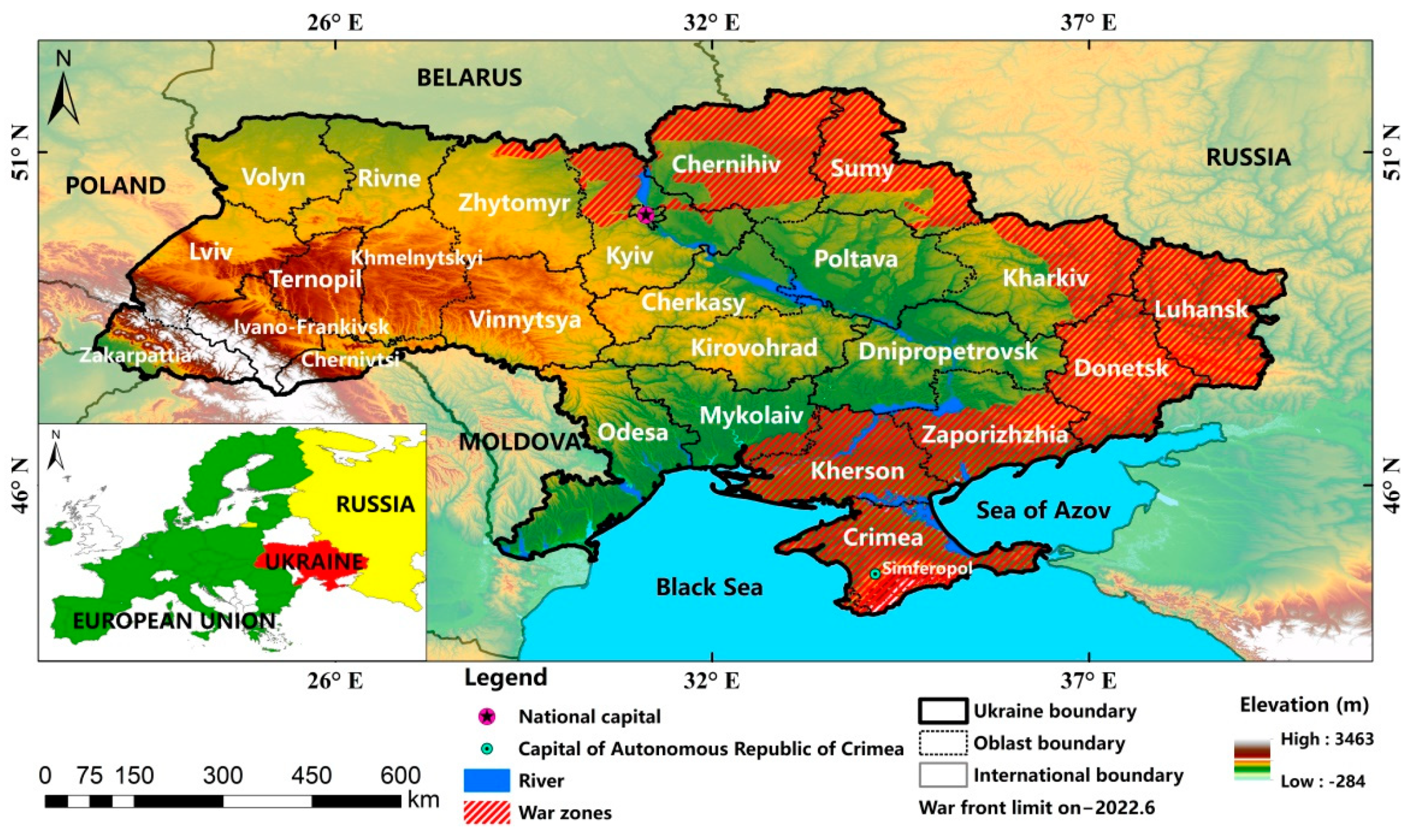
2.1. Study Area

Ukraine is a country in Eastern Europe (longitude: 31°9′56″ E; latitude: 48°22′46″ N) that covers approximately 603,500 km² and has a population of approximately 43 million people. It is divided into 24 oblasts (Cherkasy, Chernihiv, Chernivtsi, Crimea, Dnipropetrovsk, Donetsk, Ivano-Frankivsk, Kharkiv, Kherson, Khmelnytskyi, Kyiv, Kirovohrad, Luhansk, Lviv, Mykolaiv, Odesa, Poltava, Rivne, Sumy, Ternopil, Vinnytsia, Volyn, Zakarpattia, Zaporizhzhia and Zhytomyr) and one autonomous republic (Crimea) (Figure 1) [53]. Ukraine has an average elevation of about 178 m. This region has a typical humid continental climate, with an annual average precipitation of 565 mm and an annual average temperature of 7.1 °C [54]. Ukraine, as an agrarian country, is one of the largest grain exporters in the world, and its major land cover type is cropland, covering nearly half of the country’s area. Wheat, corn, soybeans, sunflower, barley, and rapeseed are the main agricultural products [55]. Ukraine regained its independence in 1991, with the dissolution of the Soviet Union. The agricultural land management pattern has shifted from collectivized towards market-oriented economies [9,10]. Large areas of agricultural cropland have been fallowed or abandoned without management because of the lack of financial support, and weeds may regrow on the cropland [23]. In addition to the problems of historical and political volatility, the ongoing Ukraine–Russia war has created the risk of food insecurity. The country’s vast agricultural areas are subjected to military occupation, which is not conducive to sowing campaigns. The war zones are shown in Figure 1, and are partitioned according to international military reports and cartographic materials up to June 2022. The affected farming area is approximately 38% of the total cropland area of Ukraine, comprising 232,300 km², which is taken into consideration in the buffer zone of the frontline territory.

2.2. Remote Sensing Satellite Imagery

Surface reflectance (SR) images from the Landsat 8 Operational Land Imager (OLI) (Collection 2, level-2) were collected from the GEE cloud computing platform from 2018 to 2022. Landsat 8 SR products have been atmospherically corrected using the Land Surface Reflectance Code (LaSRC). Clouds, cloud shadows, snow, and ice pixels were masked based on the accompanying quality assessment band. The surface reflectance values from Landsat collection 2 were calculated by multiplying the original pixel value by a scale factor of 0.0000275, and then adding an offset of −0.2 per pixel. To obtain clear and cloudless images that cover the entire study area, we filtered out Landsat images acquired from April to October 2018 to 2021, and March to June 2022.

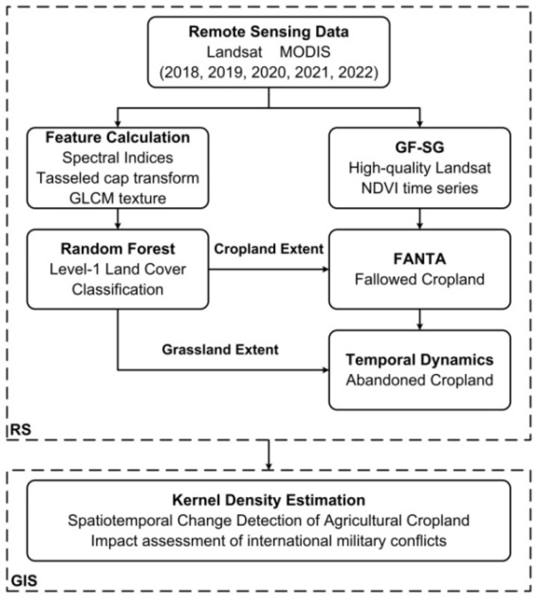
2.3. Methodological Framework

The methodology was carried out in two phases (Figure 2). First, level-1 land cover (cropland, forest, grassland, bare ground, built-up area, water, and wetland) was classified using an RF classifier with several feature variables derived from Landsat images, such as spectral indices, tasseled cap transform variables, and gray-level co-occurrence matrix texture (GLCM) variables. Five level-1 land cover classification maps were generated for the years 2018–2022. Within the cropland extent, the FANTA method was applied to map annual fallowed cropland using a high-quality NDVI time series with a 30 m spatial resolution produced by the GF-SG method by integrating Landsat and MODIS images. The abandoned cropland was extracted using two consecutive years of fallowed cropland maps. In the first phase, we used several RS algorithms to extract information on objects of interest (land cover types, fallowed cropland, and abandoned cropland) on the GEE platform. Second, we analyzed the spatial and temporal changes in agricultural croplands and assessed the impact of the ongoing Ukraine–Russia war on agricultural management practices and food security. In the second phase, we introduced the kernel density spatial analysis technology of GIS to more clearly reveal the spatial distribution pattern.

2.4. Level-1 Land Cover Classification

2.4.1. Training and Testing Sample Generation

To efficiently obtain accurate and sufficient training samples, we integrated manually labeled samples and samples automatically derived from a global land cover product. Liu et al. proposed a novel global 30 m land cover dataset that provided fine and accurate classification maps once every 5 years from 1985 to 2020 (GLC_FCS30-1985_2020) [56]. The global land cover classification product is produced by applying an RF classifier based on time series Landsat surface reflectance data, Sentinel-1 SAR data, DEM data, a global thematic auxiliary dataset, and a prior knowledge dataset on the GEE platform [56,57,58]. We adapted the fine classification system of the GLC_FCS30-1985_2020 product to be consistent with the level-1 land cover types of Ukraine owing to the actual geographical characteristics (

Table 1. Number of samples and description of class system for initial land cover classification in Ukraine.

No.	Code	Class	Training Samples			Testing Samples
			P	M2018	M2021
1	C1	Bare ground	1975	834	867	169
2	C2	Built-up area	1994	1609	1611	279
3	C3	Cropland	5002	1791	1796	322
4	C4	Forest	4975	1756	1763	116
5	C5	Grassland	2134	1106	922	271
6	C6	Wetland	1507	1376	1389	193
7	C7	Water	1811	639	634	225
Total			19,398	9111	8982	1575

P represents the training samples derived from land cover classification product data; M represents the training samples generated by manually labeling.

).

We extracted the stable pixels for which the land cover classes remained unchanged from all the GLC_FCS30-1985_2020 classification maps by using the overlay spatial analysis method in ArcGIS 10.2 software (ESRI Inc., Redlands, CA, USA). Subsequently, many points were automatically generated using stratified random sampling from the stable areas. Considering the influence of the classification errors of the product, we checked the automatically derived points and removed the observably incorrect points according to Google Earth and Landsat images. A total of 19,398 points were selected from the classification product as the training samples for classification in each year. Considering the labor cost, operational efficiency, and dynamic spatial distribution of land cover across several years, we manually labeled a total of 9111 and 8982 points from the Landsat images in 2018 and 2019, respectively, and labeled points of other years could be updated based on the two-year sample sets.

A total of 1575 points within the testing dataset used to assess the classification accuracy were manually labeled from the high-resolution images available on Google Earth. Moreover, to ensure the reliability of the testing data for assessing the historical classification results, the global ESRI land cover classification product with a 10 m spatial resolution for each year from 2017 to 2021 released by the Environmental Systems Research Institute was used as a reference to correct the testing points.

2.4.2. Random Forest Classification

The random forest classifier is an ensemble learning algorithm that integrates many classification and regression tree (CART) classifiers by using a bagging strategy. The bootstrap sampling technology is used to generate sample subsets for training each CART. During the construction of a CART, each node is split using the feature variables based on the threshold yielded from the smallest Gini coefficient [59,60]. The RF method has been widely used and proved to perform better with high-dimensional data and provide higher accuracy in classification tasks [61,62]. Furthermore, application programming interfaces (APIs) for the RF classifier have been provided to make requests to the GEE servers, allowing for the rapid completion of large-scale land cover mapping on the GEE platform. The number of decision trees (N_tree) and the number of variables per split (M_try) are important hyper-parameters of the RF classifier that can affect computational efficiency and classification accuracy. In this study, N_tree was set to 100 and the value of M_try was the square root value of the total number of input features.

We applied the RF method with several feature variables to classify level-1 land covers. The variables included surface reflectance variables derived from Landsat images (blue, green, red, near infrared, and two shortwave infrared bands); Normalized Difference Vegetation Index (NDVI), Modified Normalized Difference Water Index (MNDWI), Normalized Difference Built-up Index (NDBI), and Bare Soil Index (BSI); brightness, greenness, and wetness from a tasseled cap transform (

Table 2. Calculation equations of normalized difference indices and component variables from tasseled cap transform method.

Abbreviation	Formula
NDVI	(NIR − Red)/(NIR + Red)
MNDWI	(Green − SWIR1)/(Green + SWIR1)
NDBI	(SWIR1 − NIR)/(SWIR1 + NIR)
BSI	((SWIR2 + Red) − (NIR + Blue))/((SWIR2 + Red) + (NIR + Blue))
Brightness	0.3037 × Blue + 0.2793 × Green + 0.4743 × Red + 0.5585 × NIR × +0.5082 × SWIR1 + 0.1863 × SWIR2
Greenness	−0.2848 × Blue − 0.2435 × Green − 0.5436 × Red + 0.7243 × NIR × +0.0840 × SWIR1 − 0.1800 × SWIR2
Wetness	0.1509 × Blue + 0.1973 × Green − 0.3279 × Red + 0.3406 × NIR × −0.7112 × SWIR1 − 0.4572 × SWIR2

); and texture variables (contrast, correlation, inverse difference moment, sum average, and entropy) calculated from the gray-level co-occurrence matrix method (GLCM) using the near-infrared band that can reflect vegetation information [63,64,65].

Because of the pixel-based classification, the results may contain many scattered pixels representing misclassified pixels that directly decrease the classification accuracy and impact the continuity of spatial patterns for land cover types in the classification maps. Therefore, a post-classification process was conducted to reduce the salt-and-pepper noise in ENVI 5.1 software (Exelis Visual Information Solutions, Inc., Boulder, CO, USA). Noise pixels were removed using majority analysis, which groups the scattered pixels into the majority class within a 5 × 5 kernel size.

2.4.3. Accuracy Assessment

The confusion matrix is one of the most common methods applied to assess classification accuracy. Several evaluation indicators derived from the confusion matrix can be used to comprehensively assess the classification results, including the overall accuracy (OA), kappa coefficient (Kappa), user’s accuracy (UA), and producer’s accuracy (PA). The OA represents the total percentage correctly classified. The kappa coefficient reflects the agreement between the classification results and the actual reference data. The UA describes the percentage of correctly classified results of the classification results per class. The PA describes the percentage of correctly classified results of the actual reference sites per class [66]. The equations for calculating each indicator are as follows:

$$\mathrm{OA}={\displaystyle {\sum }_{i=1}^n{m}_{ii}}/N$$

(1)

$$\mathrm{UA}=m_{ii}/m_{i+}$$

(2)

$$\mathrm{PA}=m_{ii}/m_{+i}$$

(3)

$$\mathrm{Kappa}=\left(N{\displaystyle {\sum }_{i=1}^n{m}_{ij}}-{\displaystyle {\sum }_{i=1}^n{m}_{i+}{m}_{+i}}\right)/\left(N^2-{\displaystyle {\sum }_{i=1}^n{m}_{i+}{m}_{+i}}\right)$$

(4)

where N is the total number of testing samples; m_ii is the correctly classified pixel of class i; m_i+ is the total pixel number of class i in the data to be verified; m_+i is the total pixel number of type i in the reference data; and n is the class number.

2.5. Fallowed Cropland Classification

2.5.1. NDVI Time Series Reconstruction Method

The Landsat NDVI time series data with 30 m spatial resolution effectively reflected the vegetation phenological stages and could be used to classify croplands under different management practices [67,68]. However, due to frequent cloud contamination, unscanned gaps, and limitations of satellite 16-day revisit cycles, temporally continuous Landsat NDVI time series were difficult to obtain.

A novel reconstruction method called gap filling and Savitzky–Golay filtering (GF-SG) was recently proposed by Chen, and was used to produce Landsat NDVI time series data in this study. The GF-SG method first fills the missing values of the original Landsat NDVI time series data by using MODIS NDVI time series data to generate a cloud-free Landsat NDVI time series. The coarse spatial resolution of MODIS images is resampled using the bicubic interpolation method, which is in accordance with the spatial resolution of the Landsat images. The temporal shape curve for each Landsat image pixel is determined by searching and matching operations in the resampled MODIS image around the pixel location. The synthesized Landsat-MODIS NDVI time-series data are preliminarily generated. Second, a weighted Savitzky–Golay filter method is designed to remove residual noise and smooth the synthesized NDVI time series. Finally, cloud-free and temporally continuous Landsat NDVI time series data with 30 m spatial resolution and an 8-day period are produced [36].

Additionally, we selected the MOD09Q1 product from the GEE platform to generate MODIS time series data. MOD09Q1, corrected for atmospheric conditions, provides surface spectral reflectance of red and near-infrared at 250 m resolution. For each pixel, a value was selected from all acquisitions within the 8-day composite period. Moreover, the GF-SG method can be implemented simply using an open-source GEE code on the GEE platform. Finally, we calculated 46 NDVI images for each year from 2018 to 2021 and 28 NDVI images for January–July 2022.

2.5.2. FANTA Algorithm

The fallow-land algorithm based on neighborhood and temporal anomalies (FANTA) method is used to identify active and fallow land by using NDVI time series data, which compares the current greenness of a cropland pixel to its historical greenness and its neighborhood greenness [31,32]. Temporal anomalies (${T\_NDVI}_{max}^m$ and ${T\_NDVI}_{range}^m$) are calculated using a z-score transformation as follows:

$$T\_NDV{I}_{max}^m=\left(NDV{I}_{max}^m-NDV{I}_{max\_mean}^m\right)/NDV{I}_{max\_stdv}^m$$

(5)

$$T\_NDV{I}_{range}^m=\left(NDV{I}_{range}^m-NDV{I}_{range\_mean}^m\right)/NDV{I}_{range\_stdv}^m$$

(6)

where m is the month in the year of interest; ${NDVI}_{max}^m$ is the monthly NDVI maximum value; ${NDVI}_{range}^m$ is the monthly NDVI range value that is the difference between the maximum and minimum NDVI values. The mean, standard deviation and median values of monthly ${NDVI}_{max}^m$ and ${NDVI}_{range}^m$ are also calculated. In particular, the monthly ${NDVI}_{max}^m$ and ${NDVI}_{range}^m$ values used for calculating mean and standard deviation are greater than or equal to the median NDVI observed with the pixels between 2018 and 2022.

Spatial anomalies are calculated using z-score transformation based on the monthly NDVI maximum and monthly NDVI ranges, similar to the temporal anomalies. However, the extraction method of the median values (${S\_NDVI}_{max\_stdv}^m$ and ${S\_NDVI}_{ramge\_stdv}^m$) is different, and was calculated based on all annual pixels within a neighborhood zone. In this study, the administrative regions are used as spatial neighbor regions instead of climate divisions from the primal method because of the aim of identifying the war-driven agricultural management changes in our study.

The FANTA method uses monthly NDVI temporal and spatial anomalies to identify the fallowed cropland based on four logical statements (Equations (7)–(10)). If any two of the four logical statements were true, the pixel was classified as fallowed cropland for a given month.

Statement 1 (Equation (7)) and Statement 2 (Equation(8)) illustrate the consistently low NDVI maximum and range values of fallowed cropland, respectively, during the growing season based on temporal greenness anomalies.

$$T\_NDV{I}_{max}^{m_i}<-3(i=5,6,7) \mathrm{OR} T\_NDV{I}_{max}^{m_j}<-3(j=4,5,6)$$

(7)

$$T\_NDV{I}_{range}^{m_i}<-3(i=5,6,7) \mathrm{OR} T\_NDV{I}_{range}^{m_j}<-3(j=4,5,6)$$

(8)

where m is the month in the year of interest; ${T\_NDVI}_{max}^m$ and ${T\_NDVI}_{range}^m$ are the temporal anomalies based on the NDVI maximum and range values, respectively; i represents the main growing season in May, June, and July; and j represents the early growing season in April, May, and June.

Statement 3 (Equation (9)) and Statement 4 (Equation (10)) illustrate the consistently low NDVI maximum and range values of fallowed cropland within a neighborhood, respectively, during the main growing season based on spatial greenness anomalies.

$$\mathrm{MAX}(NDV{I}_{max}^{m_i})<0.8\mathrm{MAX}(S\_NDV{I}_{max\_stdv}^{m_i})(i=4,5,6,7)$$

(9)

$$\mathrm{MAX}(NDV{I}_{range}^{m_i})<0.8\mathrm{MAX}(S\_NDV{I}_{range\_stdv}^{m_i})(i=4,5,6,7)$$

(10)

where ${S\_NDVI}_{max\_stdv}^m$ and ${S\_NDVI}_{ramge\_stdv}^m$ are the median values of ${NDVI}_{max}^m$ and ${NDVI}_{range}^m$ that are calculated based on all annual pixels within a neighborhood zone, respectively; i represents the main growing season in April, May, June, and July.

2.6. Cropland Spatial Distribution Analysis

To reveal the spatial distribution pattern of active, fallowed, and abandoned croplands more clearly and visually, a spatial geographical analysis algorithm called kernel density estimation was applied. This method calculates the density of point features in a neighborhood around those features, and produces a continuous density surface map to show the density of objects of interest. This method is beneficial for detecting and displaying spatial hotspots and the dispersion of cropland for effectively and directly understanding spatial and temporal pattern characteristics [69,70]. In this study, the kernel density method was carried out using spatial analysis tools in ArcGIS 10.2 software. First, the raster data obtained from several fallowed and abandoned cropland classification maps were converted to polygon vector data. Then, the center points of the polygon features were extracted to execute the kernel density method. Finally, kernel density maps were obtained to assess agricultural management in the case of the ongoing Ukraine–Russia war.

3. Results

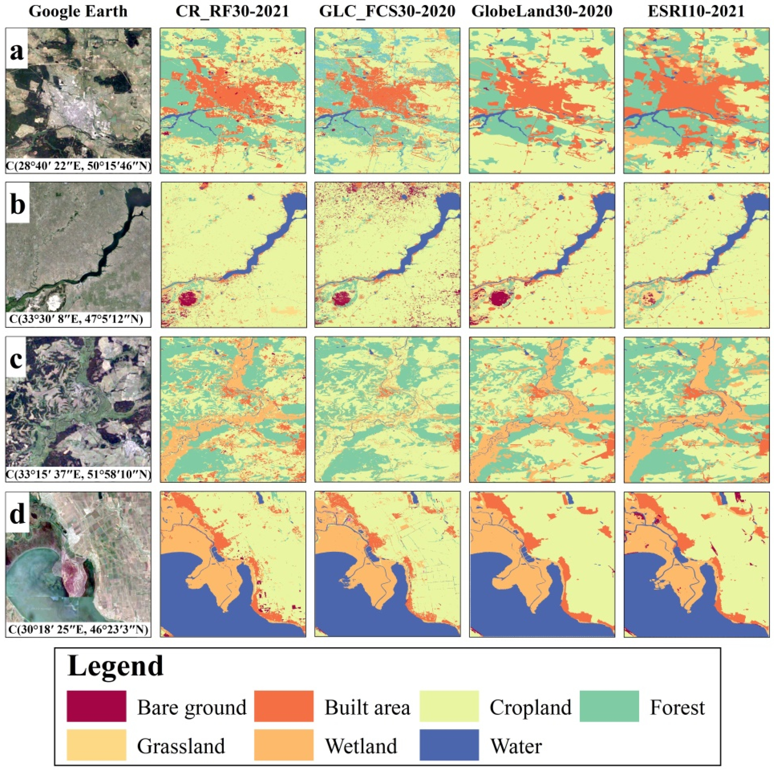
3.1. Level-1 Land Cover Classification

The RF method was applied to classify level-1 land cover types within 18 variables for each year from 2018 to 2022. The overall accuracy, kappa coefficient, producer’s accuracy, and user’s accuracy are shown in

Table 3. Accuracy evaluation results based on testing samples.

Year		C1	C2	C3	C4	C5	C6	C7	OA(%)	Kappa
2018	PA(%)	97.63	94.62	88.20	98.28	44.65	65.80	98.22	82.29	0.7904
	UA(%)	94.83	91.03	70.12	75.00	79.08	70.56	100.00
2019	PA(%)	88.76	91.40	87.58	98.28	53.14	60.10	99.56	81.59	0.7817
	UA(%)	97.40	89.47	67.95	79.17	78.26	68.64	100.00
2020	PA(%)	84.02	95.70	86.02	98.28	47.97	58.03	97.78	80.13	0.7646
	UA(%)	96.60	87.25	68.23	70.81	80.25	65.12	99.55
2021	PA(%)	85.80	95.70	90.99	95.69	55.72	77.20	98.22	84.89	0.8208
	UA(%)	96.03	89.90	71.99	86.05	90.42	74.13	99.10
2022	PA(%)	81.66	96.42	92.55	94.83	57.35	66.84	98.22	83.82	0.8081
	UA(%)	96.50	96.42	69.46	69.62	88.14	79.14	97.36

. The overall accuracy and kappa coefficient of annual land cover classification are similar, with values greater than 80% and 0.79, respectively. The RF method yielded the highest producer’s accuracy and user’s accuracy for bare ground, built-up areas, and water, approximately above 90% for each year. Forests had the highest producer’s accuracy with above 95%, whereas the user’s accuracy value was lower, ranging from 69.62 to 86.05%. RF also produced good results for the cropland used to extract the agricultural extent. The producer’s accuracy of cropland ranged from 86.02 to 92.55%, and the user’s accuracy of cropland ranged from 67.95 to 71.99%. In contrast, grasslands and wetland had lower accuracies among all classes. The producer’s and user’s accuracies of grassland were about 80% and 50%, respectively, and the classification accuracy of wetland was approximately 70%.

Figure 3 shows the visual spatial patterns of all classes based on Google Earth images, RF classification results (CR_RF30-2021), and three different land cover products. The products included GLC_FCS with 30 m spatial resolution in 2020 (GLC_FCS30-2020), GlobeLand with 30 m spatial resolution in 2020 (GlobeLand30-2020), and ESRI land cover data with 10 m spatial resolution in 2021 (ESRI10-2021). The results revealed that CR_RF30-2021 achieved desirable visual results, as demonstrated in the second column of Figure 3, which were able to better distinguish different classes within the neighborhood. The class boundaries were smooth and clear. The spatial continuity was less influenced by the scattered pixels (salt-and-pepper noise). Compared with the GLC_FCS30-2020 and GlobeLand30-2020 products, CR_RF30-2021 showed better visual classification results for bare ground, grassland, and wetland (see Figure 3b,c). Although cropland, as the most focused class, was partially misclassified as grassland and wetland, the classification results were satisfactory and can be sufficient to illustrate the actual spatial pattern compared with the high-spatial-resolution maps.

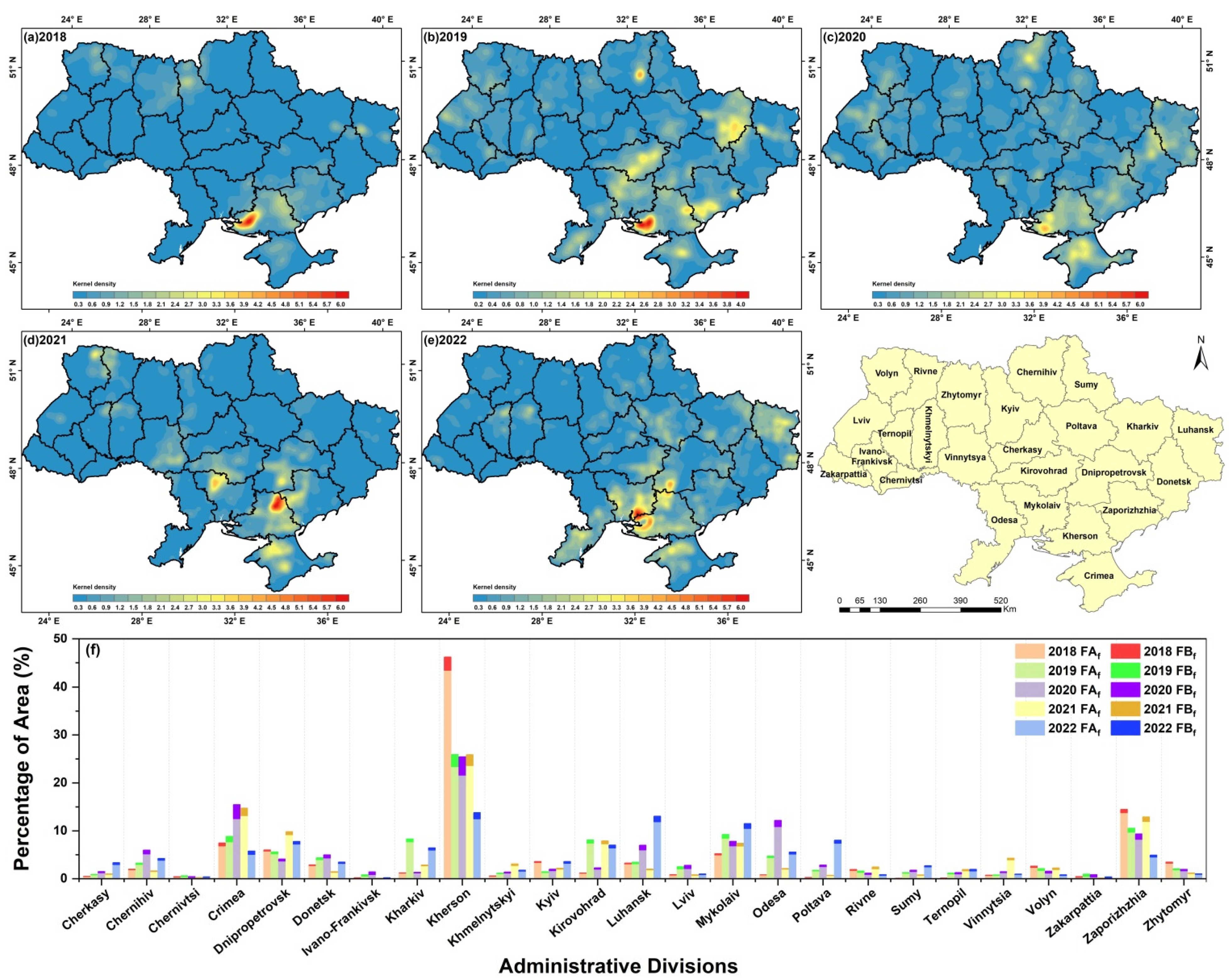
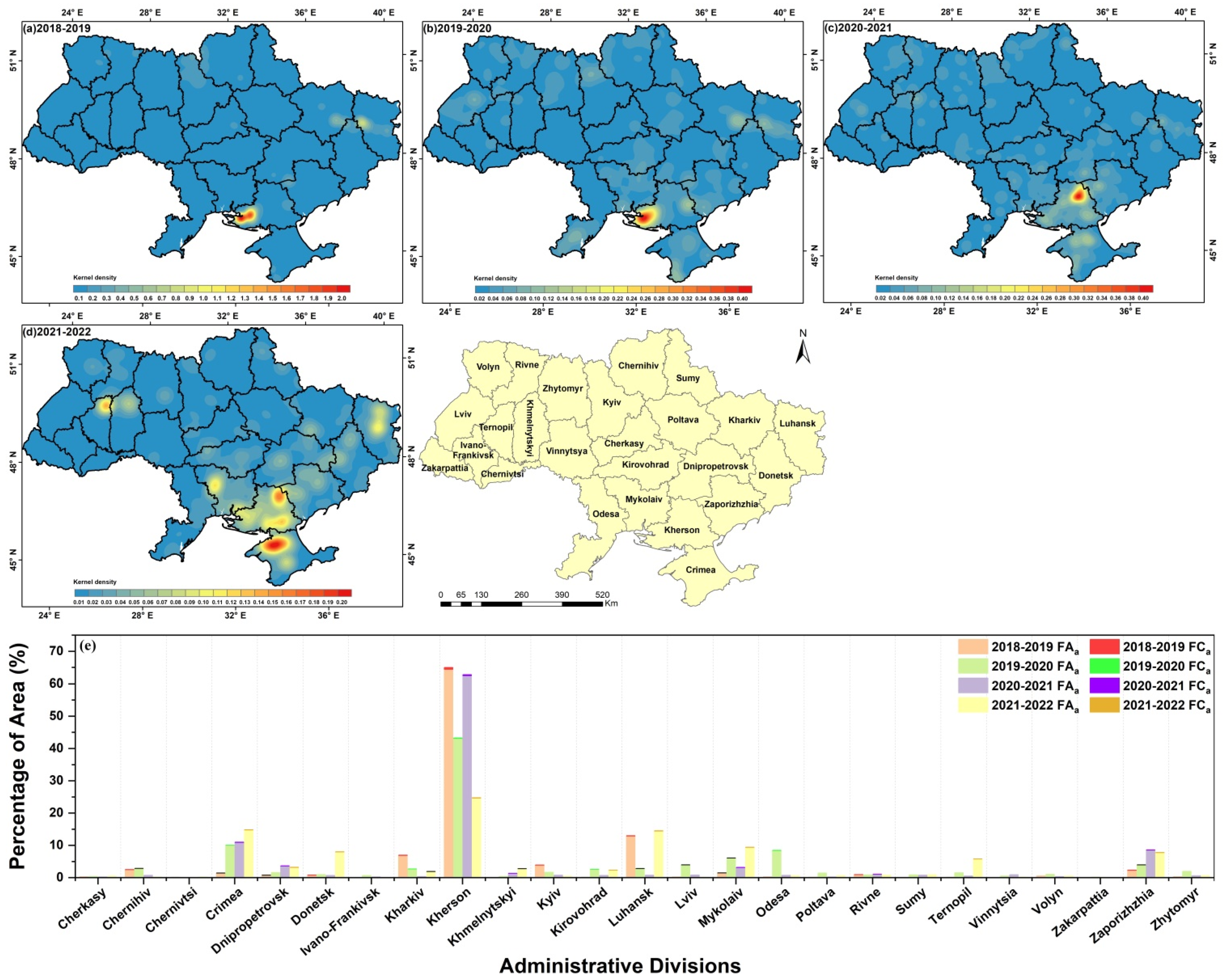
3.2. Spatial and Temporal Analysis of Fallowed and Abandoned Cropland

Fallowed cropland, defined as farmland without cultivation and management for one year, was extracted from the FANTA method. To monitor the abandoned cropland, we used fallowed cropland time series classification results to map the abandoned cropland in which the cultivatable land was not cultivated for at least two consecutive years.

Figure 4 shows that the fallowed cropland was widespread in many administrative regions, and the distribution pattern varied during the five years. The percentage of fallowed croplands fluctuated between years. The fallowed cropland was mainly concentrated in eastern Ukraine, and the highest density frequently occurred in Kherson, which accounted for 12.49–43.43% of the total fallowed cropland area of Ukraine from 2018 to 2022. Other eastern regions, such as Zaporizhzhia, Crimea, Luhansk, Kirovohrad, Dnipropetrovsk, and Mykolaiv had larger areas of fallowed croplands with an area percentage of more than 6% of total fallowed cropland for at least two years. In western Ukraine, the spatial distribution pattern of fallowed cropland was dispersed with a smaller area percentage of less than 4%. Some western regions, such as Zhytomyr, Volyn, Rivne, Lviv, and Khmehnytskyi, accounted for more than 1% of the total fallowed cropland area. The fallowed cropland area percentage of total cropland area in each administrative region was 0.01–3.84%.

Figure 5 shows that a certain area of fallowed cropland without management changed to abandoned croplands and occurred in several administrative regions with different area percentages. The hotspots frequently occurred in western Kherson, with the area percentage of total abandoned cropland varying from 24.62 to 64.39%, and also continually arose in the center of Luhansk, with the area percentage varying from 0.75 to 14.42%. Moreover, the abandoned cropland was distributed more widely in eastern Ukraine from 2021 to 2022; besides Kherson and Luhansk, some administrative regions, such as Crimea, Donetsk, Mykolaiv, and Zaporizhzhia, also had large areas of abandoned cropland, with an area percentage of more than 7% of total abandoned cropland. Abandoned cropland is also widely distributed in some regions in the northwest of Ukraine, such as Volyn, Rivne, Zhytomyr, and Kyiv, during different periods.

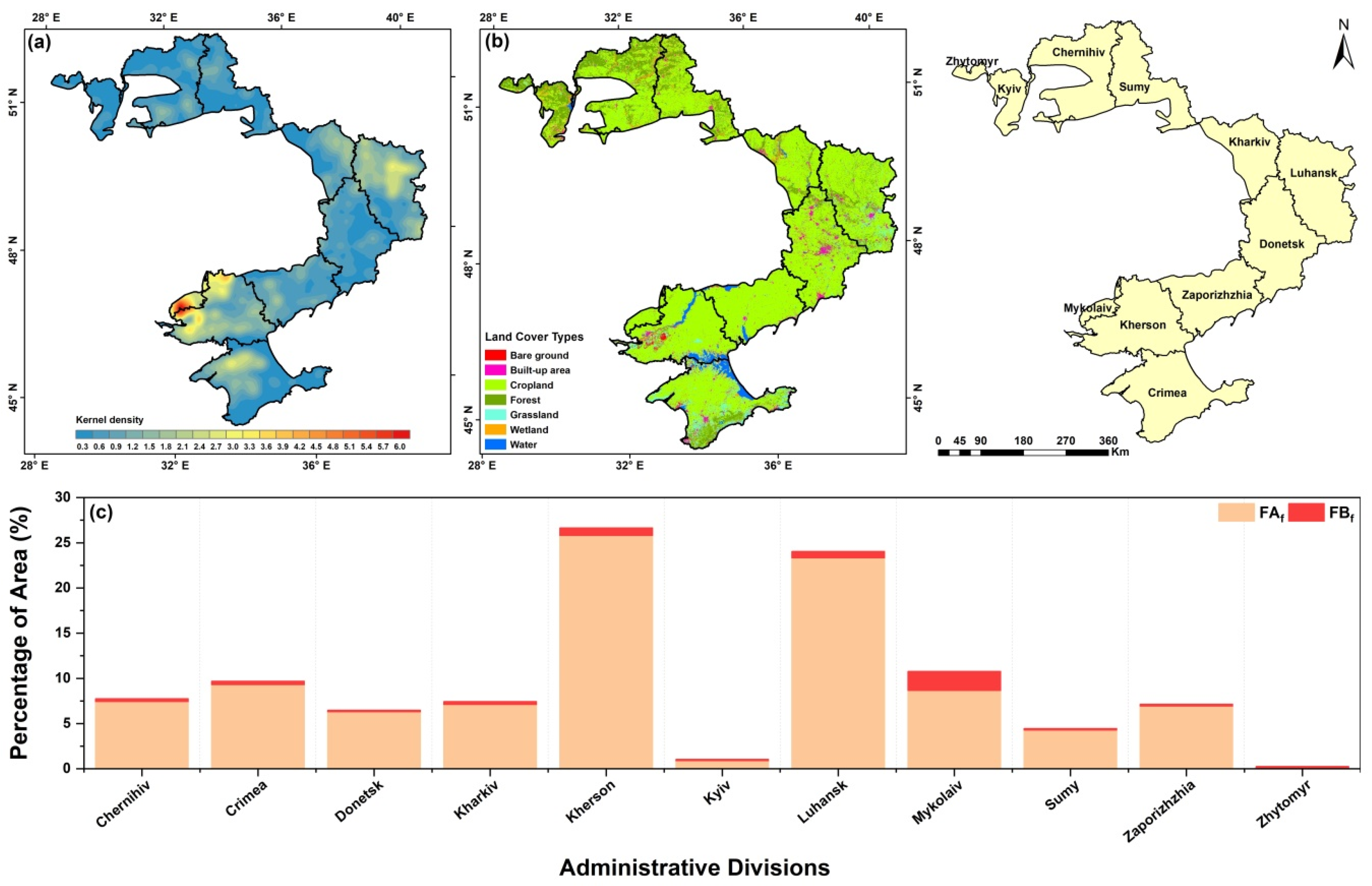
3.3. Influence of the War on Agricultural Cropland

As for the influence analysis of the war on agricultural development and management, farmland that was regularly cultivated for at least three years during 2018–2021 and only fallowed in 2022 was defined as cropland that could be severely impacted by the Ukraine–Russia war. Administrative regions that suffered from the war mainly included Chernihiv, Crimea, Donetsk, Kharkiv, Kherson, Kyiv, Luhansk, Mykolaiv, Sumy, Zaporizhzhia, and Zhytomyr, which had large areas of cropland (Figure 6b). From the kernel density map, within the confines of war zones, the agricultural management of cropland was influenced to various extents, with fallowed cropland distributed widely in all administrative regions. Western Kherson, the center of Luhansk and northern Crimea had high kernel density values, with largest area percentages of 25.35%, 22.91%, and 9.13% of the total fallowed cropland, respectively. Other administrative divisions, such as Mykolaiv, Chernihiv, Kharkiv, Zaporizhzhia, and Donetsk, had an area percentage of the total fallowed cropland with the value of approximately 6%. The fallowed cropland area percentage of total cropland area in each administrative region was 0.17–2.14%.

4. Discussion

4.1. Mapping and Analysis Approaches

To accurately and rapidly extract fallowed and abandoned land and effectively assess the influence of the war on agricultural cropland management practices in Ukraine, we applied a series of proven remote sensing and GIS techniques, including the RF classifier, GF-SG method, FANTA algorithm, and kernel density estimation; these remote sensing methods can be implemented on the GEE platform. The reasonable results adequately demonstrate the accessibility of these methods for monitoring large-scale cultivated land management patterns.

For the RF method to classify level-1 land cover types, several variables were used to provide abundant information, which helped identify the spectral, geometric, interior structure, and spatial neighborhood characteristics of different surface ground objects on Landsat 8 RS imagery. The RF classifier with these variables produced satisfactory classification accuracy for cropland, which played an important role in developing a cultivated mask layer for the following tasks. In the annual classification maps, cropland was partially misclassified as grassland and wetland owing to the spectral similarity of herbaceous vegetation and the spatially blurred boundary of adjacent classes.

The FANTA algorithm mainly depends on NDVI time series data to identify fallow land. The most prominent advantage of the FANTA algorithm is that it requires no field data for training and instead relies adequately on temporal and spatial NDVI anomalous values [31]. Using this method to map fallowed croplands is not subject to geographical conditions, climate conditions, or time cost; it may help factually reflect the historical greenness dynamics of vegetation growth and rapidly obtain estimate results to monitor the agricultural cultivated management status. The GF-SG method significantly reduced the influence of cloud contamination on Landsat images and improved the temporal resolution, resulting in high-quality Landsat NDVI time series data with 30 m spatial resolution and 8-day temporal resolution based on MODIS data [36].

Kernel density estimation is a suitable spatial analysis technology for detecting hotspots and dispersion patterns in fallowed and abandoned croplands. It can intuitively and visually reveal the areas that frequently occur as hotspots of fallowed and abandoned croplands, which should be considered for reinforcing agricultural management and increasing agricultural production [71]. The hotspots of fallowed and abandoned cropland sequentially occurring in war zones can be used as an indicator for assessing the risk of food crisis caused by the war.

A joint utilization of the RF classifier, GF-SG method, FANTA algorithm, and kernel density estimation proved beneficial for quickly monitoring and assessing agricultural cropland status in large-scale regions where it was difficult to conduct fieldwork. The practical international situation of the ongoing war in Ukraine is complicated and volatile, which increased the risk of collecting field data, and we had minimal detailed prior knowledge of Ukrainian agricultural management. The methods and implementation procedures proposed in this study can be used for the rapid and effective assessment of the impact of war on agricultural management.

4.2. Assessment of Agricultural Cropland Management Practices

The annual kernel density maps of fallowed cropland illustrated that fallow cropland management was common in Ukraine. The spatial distribution pattern of fallowed croplands was widespread and varied between years. Hotspots of fallowed cropland frequently occurred in eastern Ukraine, such as Kherson, Crimea, Luhansk, and Zakarpattia, and long-term consecutive fallow agricultural management caused cropland abandonment. Moreover, Volyn, Rivne, Zhytomyr, Kyiv, and Chernihiv, which were located in northwest Ukraine, also had widely distributed abandoned croplands.

Owing to a more direct evaluation of the influence of the war in Ukraine, we further extracted the cropland that was regularly cultivated for at least three years from 2018 to 2021 but just fallowed in 2022. The results revealed that the hotspots of cropland that were impacted by the war were found in western Kherson, the center of Luhansk, and northern Crimea. Kherson and Luhansk are the major war zones where Russian forces controlled or operated attacks without control from February to July 2022. The Autonomous Republic of Crimea is the only region within Ukraine with its own constitution. It came to be controlled by Russia on 16 March 2014, and had a sovereignty dispute between Russia and Ukraine [72]. Northern Crimea was close to the war zones of Russian control. Other oblasts, such as Zaporizhzhia, Donetsk, and Kharkiv in eastern Ukraine, and Chernihiv, Sumy, Kyiv, and Zhytormyr in northern Ukraine, had large areas of fallowed cropland, which also suffered from the Ukraine–Russia war and Ukrainian partisan warfare, which have directly affected the agricultural and economic activities of Ukraine [73].

It has been reported by FAO that these war-impacted oblasts have suffered from the highest levels of food insecurity, especially Kherson, Luhansk, Kharkiv, Chernihiv, and Sumy. The war has severely disrupted economic activities, which has caused a loss of income and increased food prices. Due to migration movement and agricultural infrastructure damaged by the ongoing war, agricultural productivity has significantly reduced and a large area of cultivatable land has become fallowed cropland without agricultural management [74]. With intensifying wars, pollutants from ordnance material explosions can seriously destroy soil, water, and the atmospheric environment, which directly influences the growth of crops and food production.

As Ukraine is one of the world’s top agricultural producers and exporters, the war could jeopardize the food security of many countries, especially those that are highly dependent on Ukraine and Russia for food and fertilizer imports [75]. Moreover, according to the historical fallowed and abandoned cropland maps, the spatial distribution of agricultural croplands without management is widespread in many oblasts and varies during different periods based on various factors such as soil quality, topography, population, climate, and agricultural and economic policies [76]. It is necessary to monitor agricultural resources and management regularly to reduce the risk of a food crisis.

5. Uncertainty and Limitations

Our study has demonstrated that the proposed methodological framework for analyzing the spatiotemporal distribution of agricultural land and assessing the impact of war on agricultural management is effective and feasible. The evaluated results can be used to support scientific assessments and decisions for food security and agricultural livelihoods. Nevertheless, some uncertain and limiting factors may impact the results, and several avenues for further improvement of these methods are possible.

First, we emphatically assessed agricultural cropland management practices from 2018 to 2022, in which the time span was comparatively shorter for cropland abandonment mapping. The extension of the evaluated period and longer-term NDVI time series data may provide more sufficient and accurate historical greenness information for cultivated land. The FANTA method can improve the identification precision of fallowed croplands. Second, owing to the limitations of geographical conditions, the lack of field data creates uncertainty in the evaluation accuracy. Actual field data on agricultural management and auxiliary data, such as soil maps, agricultural parcel abandonment rate maps and historical agricultural statistical data, can help to reduce misinterpretations of cropland management maps. Moreover, the FANTA method depends mainly on long-term statistical NDVI values with empirical parameters. Auxiliary data can be used to correct the empirical parameters to reveal the actual ground conditions more accurately. Third, the quality of Landsat imagery plays an important role in the extraction of information. Although NDVI interpolation methods effectively reduce the impact of cloud contamination, they may not completely eliminate noise. The use of multisensory data may provide additional information to ensure data accuracy. We will continue to conduct this research. If we have the opportunity to request a future partnership with Ukrainian universities in connection with the agricultural sector, we may be able to obtain accurate materials from local farmers or experts and make the results as accurate as possible.

6. Conclusions

This study proposes a feasible framework for monitoring the spatiotemporal distribution of agricultural land and assessing the impact of war on agricultural management in Ukraine using RS and GIS technology. RF, GF-SG, and FANTA algorithms were used to classify fallowed croplands based on Landsat time series data on the GEE platform. Abandoned croplands were extracted based on the change detection. The kernel density method can help clearly reveal the spatial distribution of fallowed and abandoned croplands. The successful utilization of these methods has proven beneficial for the simple and quick monitoring of the spatiotemporal characteristics of agricultural cropland status in large-scale regions where it is difficult to conduct fieldwork. The results reveal the serious negative influence of war on agricultural management and development, which can directly increase the risk of international food insecurity. This study provides an insightful way to utilize scientific technology to regularly monitor the impact of war on food security and agricultural livelihoods. It can be easily expanded to other places dealing with similar issues which could be of concern to the whole world, e.g., wars, territorial conflicts based on irredentism, or more general global changes impacting agricultural developments and their regulation factors in the future.

References

1. Becker-Reshef, I.; Justice, C.; Barker, B.; Humber, M.; Rembold, F.; Bonifacio, R.; Zappacosta, M.; Budde, M.; Magadzire, T.; Shitote, C.; et al. Strengthening agricultural decisions in countries at risk of food insecurity: The GEOGLAM Crop Monitor for Early Warning. Remote Sens. Environ. 2020, 237, 111553. [Google Scholar] [CrossRef]
2. Sweeney, S.; Ruseva, T.; Estes, L.; Evans, T. Mapping Cropland in Smallholder-Dominated Savannas: Integrating Remote Sensing Techniques and Probabilistic Modeling. Remote Sens. 2015, 7, 15295–15317. [Google Scholar] [CrossRef] [Green Version]
3. Wanyama, D.; Mighty, M.; Sim, S.; Koti, F. A spatial assessment of land suitability for maize farming in Kenya. Geocarto Int. 2019, 36, 1378–1395. [Google Scholar] [CrossRef]
4. Pinstrup-Andersen, P. Food security: Definition and measurement. Food Sec. 2009, 1, 5–7. [Google Scholar] [CrossRef]
5. Olsen, V.M.; Fensholt, R.; Olofsson, P.; Bonifacio, R.; Butsic, C.; Druce, D.; Ray, D.; Prishchepov, A.V. The impact of conflict-driven cropland abandonment on food insecurity in South Sudan revealed using satellite remote sensing. Nat. Food 2021, 2, 990–996. [Google Scholar] [CrossRef]
6. Hendrix, C.; Brinkman, H. Food Insecurity and Conflict Dynamics: Causal Linkages and Complex Feedbacks. Stability 2019, 2, 1–18. [Google Scholar] [CrossRef]
7. Wheeler, T.; Von Braun, J. Climate Change Impacts on Global Food Security. Science 2013, 341, 508–513. [Google Scholar] [CrossRef]
8. Schmidhuber, J.; Tubiello, F.N. Global food security under climate change. Proc. Natl. Acad. Sci. USA 2007, 104, 19703–19708. [Google Scholar] [CrossRef] [Green Version]
9. Baumann, M.; Kuemmerle, T.; Elbakidze, M.; Ozdogan, M.; Radelof, V.C.; Keuler, N.S.; Prishchepov, A.V.; Kruhlov, I.; Hostert, P. Patterns and drivers of post-socialist farmland abandonment in Western Ukraine. Land Use Policy 2011, 28, 552–562. [Google Scholar] [CrossRef]
10. Kuemmerle, T.; Olosson, P.; Chaskovskyy, O.; Baumann, M.; Ostapowicz, K.; Woodcock, C.E.; Houghton, R.A.; Hostert, P.; Keeton, W.S.; Radeloff, V.C. Post-Soviet farmland abandonment, forest recovery, and carbon sequestration in western Ukraine. Glob. Change Biol. 2011, 17, 1335–1349. [Google Scholar] [CrossRef]
11. Moklyachuk, L.; Furdychko, O.; Pinchuk, V.; Mokliachuk, O.; Draga, M. Nitrogen balance of crop production in Ukraine. J. Environ. Manag. 2019, 246, 860–867. [Google Scholar] [CrossRef]
12. Gallego, F.J.; Kussul, N.; Skakun, S.; Kravchenko, O.; Shelestov, A.; Kussul, O. Efficiency assessment of using satellite data for crop area estimation in Ukraine. Int. J. Appl. Earth Obs. Geoinf. 2014, 29, 22–30. [Google Scholar] [CrossRef]
13. Liu, X.B.; Burras, C.L.; Kravchenko, Y.S.; Duran, A.; Huffman, T.; Morras, H.; Studdert, G.; Zhang, X.Y.; Cruse, R.M.; Yuan, X.H. Overview of Mollisols in the world: Distribution, land use and management. Can. J. Soil Sci. 2012, 92, 383–402. [Google Scholar] [CrossRef]
14. Kussul, N.; Lemoine, G.; Gallego, F.J.; Skakun, S.V.; Lavreniuk, M.; Shelestov, A.Y. Parcel-Based Crop Classification in Ukraine Using Landsat-8 Data and Sentinel-1A Data. IEEE J. Sel. Top. Appl. Earth Obs. Remote Sens. 2016, 9, 2500–2508. [Google Scholar] [CrossRef]
15. Alcantara, C.; Kuemmerle, T.; Baumann, M.; Bragina, E.V.; Griffiths, P.; Hostert, P.; Knorn, J.; Müller, D.; Prishchepov, A.V.; Schierhorn, F.; et al. Mapping the extent of abandoned farmland in Central and Eastern Europe using MODIS time series satellite data. Environ. Res. Lett. 2013, 8, 035035. [Google Scholar] [CrossRef]
16. Eklund, L.; Degerald, M.; Brandt, M.; Prishchepov, A.V.; Pilesjö, P. How conflict affects land use: Agricultural activity in areas seized by the Islamic State. Environ. Res. Lett. 2017, 12, 054004. [Google Scholar] [CrossRef] [Green Version]
17. Witmer, F.D.W. Detecting war-induced abandoned agricultural land in northeast Bosnia using multispectral, multitemporal Landsat TM imagery. Int. J. Remote Sens. 2008, 29, 3805–3831. [Google Scholar] [CrossRef]
18. He, Y.; Butsic, V.; Buchner, J.; Kuemmerle, T.; Prishchepov, A.V.; Baumann, M.; Bragina, E.V.; Sayadyan, H.; Radeloff, V.C. Agricultural abandonment and re-cultivation during and after the Chechen Wars in the northern Caucasus. Glob. Environ. Chang. 2019, 55, 149–159. [Google Scholar] [CrossRef] [Green Version]
19. He, Y.; Brandão, A.J.; Buchner, J.; Helmers, D.; Iuliano, B.G.; Kimambo, N.E.; Lewińska, K.E.; Razenkova, E.; Rizayeva, A.; Rogova, N.; et al. Monitoring cropland abandonment with Landsat time series. Remote Sens. Environ. 2020, 246, 11873. [Google Scholar] [CrossRef]
20. Skakun, S.V.; Justice, C.O.; Kussul, N.; Shelestov, A.; Lavreniuk, M. Satellite Data Reveal Cropland Losses in South-Eastern Ukraine Under Military Conflict. Front. Earth Sci. 2019, 7, 305. [Google Scholar] [CrossRef] [Green Version]
21. Estel, S.; Kuemmerle, T.; Alcántara, C.; Levers, C.; Prishchepov, A.; Hostert, P. Mapping farmland abandonment and recultivation across Europe using MODIS NDVI time series. Remote Sens. Environ. 2015, 163, 312–325. [Google Scholar] [CrossRef]
22. Alcantara, C.; Kuemmerle, T.; Prishchepov, A.V.; Radeloff, V.C. Mapping abandoned agriculture with multi-temporal MODIS satellite data. Remote Sens. Environ. 2012, 124, 334–347. [Google Scholar] [CrossRef]
23. Schierhorn, F.; Müller, D.; Beringer, T.; Prishchepov, A.V.; Kuemmerle, T.; Balmann, A. Post-Soviet cropland abandonment and carbon sequestration in European Russia, Ukraine, and Belarus. Glob. Biogeochem. Cycles 2013, 27, 1175–1185. [Google Scholar] [CrossRef]
24. Stefanski, J.; Kuemmerle, T.; Chaskovskyy, O.; Griffiths, P.; Havryluk, V.; Knorn, J.; Korol, N.; Sieber, A.; Waske, B. Mapping Land Management Regimes in Western Ukraine Using Optical and SAR Data. Remote Sens. 2014, 6, 5279–5305. [Google Scholar] [CrossRef] [Green Version]
25. Skriver, H.; Mattia, F.; Satalino, G.; Balenzano, A.; Pauwels, V.; Verhoest, N.; Davidson, M. Crop classification using short-revisit multitemporal SAR data. IEEE J. Sel. Top. Appl. Earth Obs. Remote Sens. 2011, 4, 423–431. [Google Scholar] [CrossRef]
26. Skakun, S.; Kussul, N.; Shelestov, A.Y.; Lavreniuk, M.; Kussul, O. Efficiency Assessment of Multitemporal C-Band Radarsat-2 Intensity and Landsat-8 Surface Reflectance Satellite Imagery for Crop Classification in Ukraine. IEEE J. Sel. Top. Appl. Earth Obs. Remote Sens. 2016, 9, 3712–3719. [Google Scholar] [CrossRef]
27. Atzberger, C. Advances in remote sensing of agriculture: Context description, existing operational monitoring systems and major information needs. Remote Sens. 2013, 5, 949–981. [Google Scholar] [CrossRef] [Green Version]
28. Sieber, A.; Kuemmerle, T.; Prishchepov, A.V.; Wendland, K.J.; Baumann, M.; Radeloff, V.C.; Baskin, L.M.; Hostert, P. Landsat-based mapping of post-Soviet land-use change to assess the effectiveness of the Oksky and Mordovsky protected areas in European Russia. Remote Sens. Environ. 2013, 133, 38–51. [Google Scholar] [CrossRef]
29. Elbersen, B.S.; Beaufoy, G.; Jones, G.; Noij, I.G.A.M.; van Doorn, A.M.; Breman, B.C.; Hazeu, G.W. Aspects of Data on Diverse Relationships between Agriculture and the Environment; Alterra: Wageningen, The Netherlands, 2014; pp. 102–116. [Google Scholar]
30. Stefanski, J.; Chaskovskyy, O.; Waske, B. Mapping and monitoring of land use changes in post-Soviet western Ukraine using remote sensing data. Appl. Geogr. 2014, 55, 155–164. [Google Scholar] [CrossRef]
31. Wallace, C.S.A.; Thenkabail, P.; Rodriguez, J.R.; Brown, M.K. Fallow-land Algorithm based on Neighborhood and Temporal Anomalies (FANTA) to map planted versus fallowed croplands using MODIS data to assist in drought studies leading to water and food security assessments. GISci. Remote Sens. 2017, 54, 258–282. [Google Scholar] [CrossRef]
32. Norton, C.L.; Dannenberg, M.L.; Yan, D.; Wallace, C.S.A.; Rodriguez, J.R.; Munson, S.M.; Leeuwen, W.J.D.; Smith, W.K. Climate and Socioeconomic Factors Drive Irrigated Agriculture Dynamics in the Lower Colorado River Basin. Remote Sens. 2021, 13, 1659. [Google Scholar] [CrossRef]
33. Cao, R.; Shen, M.; Zhou, J.; Chen, J. Modeling vegetation green-up dates across the Tibetan Plateau by including both seasonal and daily temperature and precipitation. Agric. For. Meteorol. 2018, 249, 176–186. [Google Scholar] [CrossRef]
34. Gao, F.; Anderson, M.C.; Zhang, X.; Yang, Z.; Alfieri, J.G.; Kustas, W.P.; Mueller, R.; Johnson, D.M.; Prueger, J.H. Toward mapping crop progress at field scales through fusion of Landsat and MODIS imagery. Remote Sens. Environ. 2017, 188, 9–25. [Google Scholar] [CrossRef] [Green Version]
35. Heck, E.; de Beurs, K.M.; Owsley, B.C.; Henebry, G.M. Evaluation of the MODIS collections 5 and 6 for change analysis of vegetation and land surface temperature dynamics in North and South America. ISPRS J. Photogramm. Remote Sens. 2019, 156, 121–134. [Google Scholar] [CrossRef]
36. Chen, Y.; Cao, R.; Chen, J.; Liu, L.; Matsushita, B. A practical approach to reconstruct high-quality Landsat NDVI time-series data by gap filling and the Savitzky–Golay filter. ISPRS J. Photogramm. Remote Sens. 2021, 180, 174–190. [Google Scholar] [CrossRef]
37. Cao, R.; Chen, Y.; Chen, J.; Zhu, X.; Shen, M. Thick cloud removal in Landsat images based on autoregression of Landsat time-series data. Remote Sens. Environ. 2020, 249, 112001. [Google Scholar] [CrossRef]
38. Ju, J.; Roy, D.P. The availability of cloud-free Landsat ETM+ data over the conterminous United States and globally. Remote Sens. Environ. 2008, 112, 1196–1211. [Google Scholar] [CrossRef]
39. Zhu, Z.; Woodcock, C.E. Object-based cloud and cloud shadow detection in Landsat imagery. Remote Sens. Environ. 2012, 118, 83–94. [Google Scholar] [CrossRef]
40. Brooks, E.B.; Thomas, V.A.; Wynne, R.H.; Coulston, J.W. Fitting the multitemporal curve: A Fourier series approach to the missing data problem in remote sensing analysis. IEEE Trans. Geosci. Remote Sens. 2012, 50, 3340–3353. [Google Scholar] [CrossRef] [Green Version]
41. Hwang, T.; Song, C.; Bolstad, P.V.; Band, L.E. Downscaling real-time vegetation dynamics by fusing multi-temporal MODIS and Landsat NDVI in topographically complex terrain. Remote Sens. Environ. 2011, 115, 2499–2512. [Google Scholar] [CrossRef]
42. Yan, L.; Roy, D.P. Large-area gap filling of Landsat reflectance time series by spectral-angle-mapper based spatio-temporal similarity (SAMSTS). Remote Sens. 2018, 10, 609. [Google Scholar] [CrossRef] [Green Version]
43. Zhu, X.; Helmer, E.H.; Gao, F.; Liu, D.; Chen, J.; Lefsky, M.A. A flexible spatiotemporal method for fusing satellite images with different resolution. Remote Sens. Environ. 2016, 172, 165–177. [Google Scholar] [CrossRef]
44. Thanh Noi, P.; Kappas, M. Comparison of random forest, k-nearest neighbor, and support vector machine classifiers for land cover classification using Sentinel-2 imagery. Sensors 2017, 18, 18. [Google Scholar] [CrossRef] [Green Version]
45. Talukdar, S.; Singha, P.; Mahato, S.; Pal, S.; Liou, Y.A.; Rahman, A. Land-use land-cover classification by machine learning classifiers for satellite observations—A review. Remote Sens. 2020, 12, 1135. [Google Scholar] [CrossRef] [Green Version]
46. Phan, T.N.; Kuch, V.; Lehnert, L.W. Land Cover Classification using Google Earth Engine and Random Forest Classifier—The Role of Image Composition. Remote Sens. 2020, 12, 2411. [Google Scholar] [CrossRef]
47. Ghorbanian, A.; Kakooei, M.; Amani, M.; Mahdavi, S.; Mohammadzadeh, A.; Hasanlou, M. Improved land cover map of Iran using Sentinel imagery within Google Earth Engine and a novel automatic workflow for land cover classification using migrated training samples. ISPRS J. Photogramm. Remote Sens. 2020, 167, 276–288. [Google Scholar] [CrossRef]
48. Orimoloye, I.R.; Ololade, O.O. Spatial evaluation of land-use dynamics in gold mining area using remote sensing and GIS technology. Int. J. Environ. Sci. Technol. 2020, 17, 4465–4480. [Google Scholar] [CrossRef]
49. Yasir, M.; Sheng, H.; Fan, H.; Nazir, S.; Niang, A.J.; Salauddin, M.; Khan, S. Automatic coastline extraction and changes analysis using remote sensing and GIS technology. IEEE Access 2020, 8, 180156–180170. [Google Scholar] [CrossRef]
50. Wu, Q.; Li, H.Q.; Wang, R.S.; Paulussen, J.; He, Y.; Wang, M.; Wang, B.H.; Wang, Z. Monitoring and predicting land use change in Beijing using remote sensing and GIS. Landsc. Urban Plan. 2006, 78, 322–333. [Google Scholar] [CrossRef]
51. Musole, M.S.B.; Ololade, O.O.; Sokolic, F. Characterisation of invasive plant proliferation within remnant riparian green corridors in Lusaka District of Zambia using Sentinel-2 imagery. Remote Sens. Appl. 2019, 15, 100245. [Google Scholar] [CrossRef]
52. Busayo, E.T.; Kalumba, A.M.; Orimoloye, I.R. Spatial planning and climate change adaptation assessment: Perspectives from Mdantsane Township dwellers in South Africa. Habitat Int. 2019, 90, 101978. [Google Scholar] [CrossRef]
53. Lavreniuk, M.; Kussul, N.; Skakun, S.; Shelestov, A.; Yailymov, B. Regional retrospective high resolution land cover for Ukraine: Methodology and results. In Proceedings of the 2015 IEEE International Geoscience and Remote Sensing Symposium (IGARSS), Milan, Italy, 26–31 July 2015; pp. 3965–3968. [Google Scholar]
54. Kussul, N.; Lavreniuk, M.; Shelestov, A.; Skakun, S. Crop inventory at regional scale in Ukraine: Developing in season and end of season crop maps with multi-temporal optical and SAR satellite imagery. Eur. J. Remote Sens. 2018, 51, 627–636. [Google Scholar] [CrossRef] [Green Version]
55. Kussul, N.; Skakun, S.; Shelestov, A.; Lavreniuk, M.; Yailymov, B.; Kussul, O. Regional scale crop mapping using multi-temporal satellite imagery. In Proceedings of the 2015 36th International Symposium on Remote Sensing of Environment, Berlin, Germany, 11–15 May 2015; pp. 11–15. [Google Scholar]
56. Zhang, X.; Liu, L.; Chen, X.; Gao, Y.; Xie, S.; Mi, J. GLC_FCS30: Global land-cover product with fine classification system at 30 m using time-series Landsat imagery. Earth Syst. Sci. Data 2021, 12, 2753–2776. [Google Scholar] [CrossRef]
57. Zhang, X.; Liu, L.; Wu, C.; Chen, X.; Gao, Y.; Xie, S.; Zhang, B. Development of a global 30 m impervious surface map using multisource and multitemporal remote sensing datasets with the Google Earth Engine platform. Earth Syst. Sci. Data 2020, 12, 1625–1648. [Google Scholar] [CrossRef]
58. Gao, Y.; Liu, L.; Zhang, X.; Chen, X.; Mi, J.; Xie, S. Consistency analysis and accuracy assessment of three global 30-m land-cover products over the European Union using the LUCAS dataset. Remote Sens. 2020, 12, 3479. [Google Scholar] [CrossRef]
59. Breiman, L. Random forests. Mach. Learn. 2001, 45, 5–32. [Google Scholar] [CrossRef] [Green Version]
60. Breiman, L.; Friedman, J.H.; Olshen, R.A.; Stone, C.J. Classification and Regression Trees (CART). Biometrics 1984, 40, 358. [Google Scholar] [CrossRef] [Green Version]
61. Wu, Q.; Zhong, R.; Zhao, W.; Song, K.; Du, L. Land-cover classification using GF-2 images and airborne lidar data based on Random Forest. Int. J. Remote Sens. 2019, 40, 2410–2426. [Google Scholar] [CrossRef]
62. Hayes, M.M.; Miller, S.N.; Murphy, M.A. High-resolution landcover classification using Random Forest. Remote Sens. Lett. 2014, 5, 112–121. [Google Scholar] [CrossRef]
63. Crist, E.P. A TM tasseled cap equivalent transformation for reflectance factor data. Remote Sens. Environ. 1985, 17, 301–306. [Google Scholar] [CrossRef]
64. Haralick, R.M.; Shanmugam, K.; Dinstein, I.H. Textural features for image classification. IEEE Trans. Syst. Man Cybern. 1973, 11, 610–621. [Google Scholar] [CrossRef] [Green Version]
65. Shijin Kumar, P.S.; Dharun, V.S. Extraction of texture features using GLCM and shape features using connected regions. Int. J. Eng. Technol. 2016, 8, 2926–2930. [Google Scholar] [CrossRef] [Green Version]
66. Rossiter, D.G. Technical Note: Statistical Methods for Accuracy Assessment of Classified Thematic Maps. Department of Earth Systems Analysis; International Institute for Geo-Information Science & Earth Observation (ITC): Enschede, The Netherlands, 2004. [Google Scholar]
67. Zhang, X.Y.; Liu, L.L.; Liu, Y.; Jayavelu, S.; Wang, J.M.; Moon, M.; Henebry, G.M.; Friedl, M.A.; Schaaf, C.B. Generation and evaluation of the VIIRS land surface phenology product. Remote Sens Environ. 2018, 216, 212–229. [Google Scholar] [CrossRef]
68. Pengra, B.; Long, J.; Dahal, D.; Stehman, S.V.; Loveland, T.R. A global reference database from very high resolution commercial satellite data and methodology for application to Landsat derived 30m continuous field tree cover data. Remote Sens Environ. 2015, 165, 234–248. [Google Scholar] [CrossRef]
69. Yang, J.; Zhu, J.; Sun, Y.; Zhao, J. Delimitating urban commercial central districts by combining kernel density estimation and road intersections: A case study in Nanjing city, China. ISPRS Int. J. Geo-Inf. 2019, 8, 93. [Google Scholar] [CrossRef] [Green Version]
70. Thanh Toan, D.T.; Hu, W.; Quang Thai, P.; Ngoc Hoat, L.; Wright, P.; Martens, P. Hot spot detection and spatio-temporal dispersion of dengue fever in Hanoi, Vietnam. Global Health Action 2013, 6, 18632. [Google Scholar] [CrossRef] [PubMed] [Green Version]
71. Mala, S.; Jat, M.K. Geographic information system based spatio-temporal dengue fever cluster analysis and mapping. Egypt. J. Remote Sens. Space Sci. 2019, 22, 297–304. [Google Scholar] [CrossRef]
72. Bebier, A. Crimea and the Russian-Ukrainian conflict. Romanian J. Eur. Aff. 2015, 15, 35–54. [Google Scholar]
73. Big-Alabo, T.; MacAlex-Achinulo, E.C. Russia-Ukraine Crisis and Regional Security. Int. J. Political Sci. 2022, 8, 21–35. [Google Scholar] [CrossRef]
74. FAO. Ukraine: Note on the Impact of the War on Food Security in Ukraine; FAO: Rome, Italy, 2022; Volume 22, pp. 1–9. [Google Scholar] [CrossRef]
75. Information Note: The Importance of Ukraine and the Russian Federation for Global Agricultural Markets and the Risks Associated with the Current Conflict. Available online: https://www.fao.org/3/cb9236en/cb9236en.pdf (accessed on 25 March 2022).
76. Smaliychuk, A.; Müller, D.; Prishchepov, A.V.; Levers, C.; Kruhlov, I.; Kuemmerle, T. Recultivation of abandoned agricultural lands in Ukraine: Patterns and drivers. Global Environ. Change 2016, 38, 70–81. [Google Scholar] [CrossRef]
Figure 1. Study region map of Ukraine with respect to war zones and elevation.
Land 11 01810 g001
Figure 2. Flowchart of mapping agricultural land, analyzing the spatiotemporal change of agricultural cropland and assessing the war impact.
Land 11 01810 g002
Figure 3. Four representative subsets (ad) for comparing the RF classification results with three land cover products and Google Earth images. The first column shows the Google Earth image, the second column shows the RF classification results named CR_RF30-2021, the following columns illustrate the classification products named GLC_FCS30-2020, GlobeLand30-2020, and ESRI10-2021. C (longitude, latitude) represents the central geographic coordinate of the enlarged pictures.
Land 11 01810 g003
Figure 4. (ae) illustrate the annual kernel density maps of fallowed cropland from 2018 to 2022; (f) illustrates the statistical graph of area percentage of fallowed cropland. FAf represents the area of fallowed cropland in each administrative region as a percentage of the total fallowed cropland area in Ukraine. FBf represents the area of fallowed cropland as a percentage of the cropland area in each administrative region.
Land 11 01810 g004
Figure 5. (ad) illustrate the kernel density maps of abandoned cropland for each consecutive two-year period from 2018 to 2022; (e) illustrates the statistical graph of area percentage of abandoned cropland. FAa represents the area of abandoned cropland in each administrative region as a percentage of the total abandoned cropland area in Ukraine. FCa represents the area of abandoned cropland as a percentage of the total fallowed cropland area in each administrative region.
Land 11 01810 g005
Figure 6. (a) illustrates the kernel density map of fallowed cropland in war zones; (b) illustrates the level-1 land cover classification map of the war zones; (c) illustrates the statistical graph of area percentage of fallowed cropland. FAf represents the area of fallowed cropland in each administrative region as a percentage of the total fallowed cropland area in war zones. FBf represents the area of fallowed cropland as a percentage of the cropland area in each administrative region.
Land 11 01810 g006