Development and Assessment of GIS-Based Landslide Susceptibility Mapping Models Using ANN, Fuzzy-AHP, and MCDA in Darjeeling Himalayas, West Bengal, India

Abstract

Landslides, a natural hazard, can endanger human lives and gravely affect the environment. A landslide susceptibility map is required for managing, planning, and mitigating landslides to reduce damage. Various approaches are used to map landslide susceptibility, with varying degrees of efficacy depending on the methodology utilized in the research. An analytical hierarchy process (AHP), a fuzzy-AHP, and an artificial neural network (ANN) are utilized in the current study to construct maps of landslide susceptibility for a part of Darjeeling and Kurseong in West Bengal, India. On a landslide inventory map, 114 landslide sites were randomly split into training and testing with a 70:30 ratio. Slope, aspect, profile curvature, drainage density, lineament density, geomorphology, soil texture, land use and land cover, lithology, and rainfall were used as model inputs. The area under the curve (AUC) was used to examine the models. When tested for validation, the ANN prediction model performed best, with an AUC of 88.1%. AUC values for fuzzy-AHP and AHP are 86.1% and 85.4%, respectively. According to the statistics, the northeast and eastern portions of the study area are the most vulnerable. This map might help development in the area by preventing human and economic losses.

1. Introduction

A common natural disaster that specifically affects steep areas and damages both the environment and human life is the landslide [1,2,3]. In addition to being a significant factor in landscape change, landslides are a cascading geohazard that can considerably impact people’s lives and habitations everywhere [4]. Landslide is the term that defines the downfall of soil or rock [5]. Landslides’ socioeconomic effects have recently worsened due to unplanned development projects, climate change, and worldwide economic growth [6,7,8]. A global report says that more than 3876 landslides happened from 1995 to 2014, by which nearly 163,658 human losses and 11,689 injuries were recorded [9]. Another record says about 55,000 lives were lost worldwide due to landslides between the years from 2004 to 2016 [10]. Due to their devastating nature and socioeconomic effects, risks related to landslides and associated phenomena have been well investigated. Susceptibility maps are the key component of hazardous damage assessment and mitigation plans in regions at high risk of landslides [8,11,12]. At the regional or watershed scale, these methods are often used in landslide assessments and mitigation. It is beneficial to identify and designate landslide-prone places using geographic information system (GIS) technologies for the purpose of constructing a geographic database of landslide inventory. The landslide conditioning factor (LCF), or geographic attributes of landslide areas that may influence potential slope stability, can be assembled into a database using GIS data sources (e.g., slope, aspect, soil texture, drainage density, rainfall, lithological type and geomorphology, etc.). In an effort to predict the risk of landslides in the future, the LCF data may be used to anticipate the behaviors of additional slopes in the study location.

Decision-makers and local authorities utilize landslide susceptibility mapping (LSM) to segment the topographical region into zones with varying degrees of susceptibility. The management and reduction of risks related to present and potential future landslides depend on this procedure, often known as “landslide risk zoning”. Using a GIS application can improve spatial data handling and provide you with more processing power [13]. Consequently, numerous quantitative methodologies and applications have been developed for LSM. Statistical models, heuristic-based models, physically based models, and, nowadays, machine learning (ML) modeling are the four main types of LSM approaches [14,15,16,17]. It has been established that each of these distinct approaches has advantages and restrictions of its own. Statistical models are suited to large areas with geotechnical parameters, but physically based models are ideal for small-scale areas with proper data availability for mapping and analysis. These models, widely used to forecast imminent slope failure, rely on a complete understanding of the landslide system obtained from surrounding surface and subsurface inspections and tracking systems. [18]. Physically based models, on the other hand, need a lot of precise data to produce accurate results for extensive study (i.e., basin-scale up to county level), which comes at a high expense both financially and computationally. Therefore, broad area risk zonation exercises cannot yet be conducted using physical-based models; as a result, during the past 40 years, the subject of LSM has been dominated by statistical and knowledge-based models, both of which are influenced by a lack of data on the terrain and environmental variables [6]. In opinion-driven models (e.g., the analytical hierarchy process (AHP)), the landslide conditioning elements are ranked and/or weighted depending on expert judgment and expertise after the model has been constructed with limited information. Since it might be challenging to evaluate or quantify a result objectively, this approach may be problematic. A variety of quantitative models have been devised and successfully utilized for modeling landslides in order to better understand landslide patterns and triggering processes. The developments in GIS over the past ten years have benefitted statistical models the most [11]. The advancement in our understanding of landslide susceptibility since the inception of statistical predictive modeling has been startlingly quick. Throughout the preceding two decades, a range of landslide susceptibility models from various statistical approaches was utilized in the ML context to create exact risk zonation maps. Many authors have used these methods for landslide mappings, such as in the identification of forested landslides with DTM derivatives using data segmentation and support vector machine (SVM) [19]; in the automatic detection of landslides with convolutional neural networks (CNN) and the identification of texture changes after and before a landslide using optical images [20]; and in the evaluation of the performance of SVM, random forest (RF), ANN, and CNN [16,21,22]. The benefit of ANN is its capacity to identify patterns with high variability through the use of hidden layers. Additionally, ANN’s excellent prediction rate and generalizability allow it to surpass established techniques such as SVM [23].

The project aims to create an ANN model for LSM and continually evaluate how well it performs against more traditional methods, such as AHP and fuzzy-AHP, to categorize subjects into various susceptibility groups. To assess the models, the receiver operating characteristic (ROC) is used. We think that local government decision-makers and site planners may use the results of our analysis to lower the danger of landslides in the region.

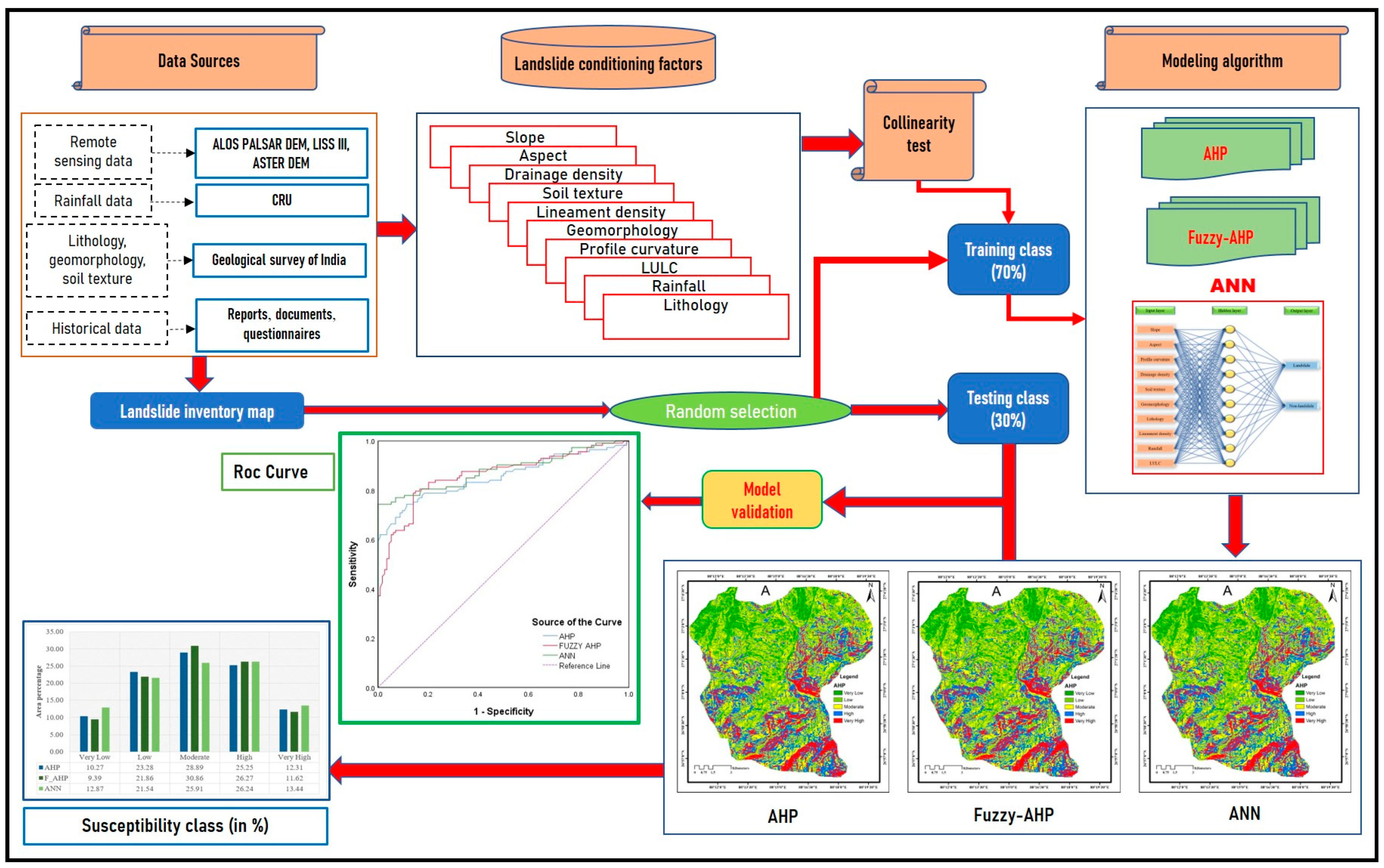
2. Materials and Methods

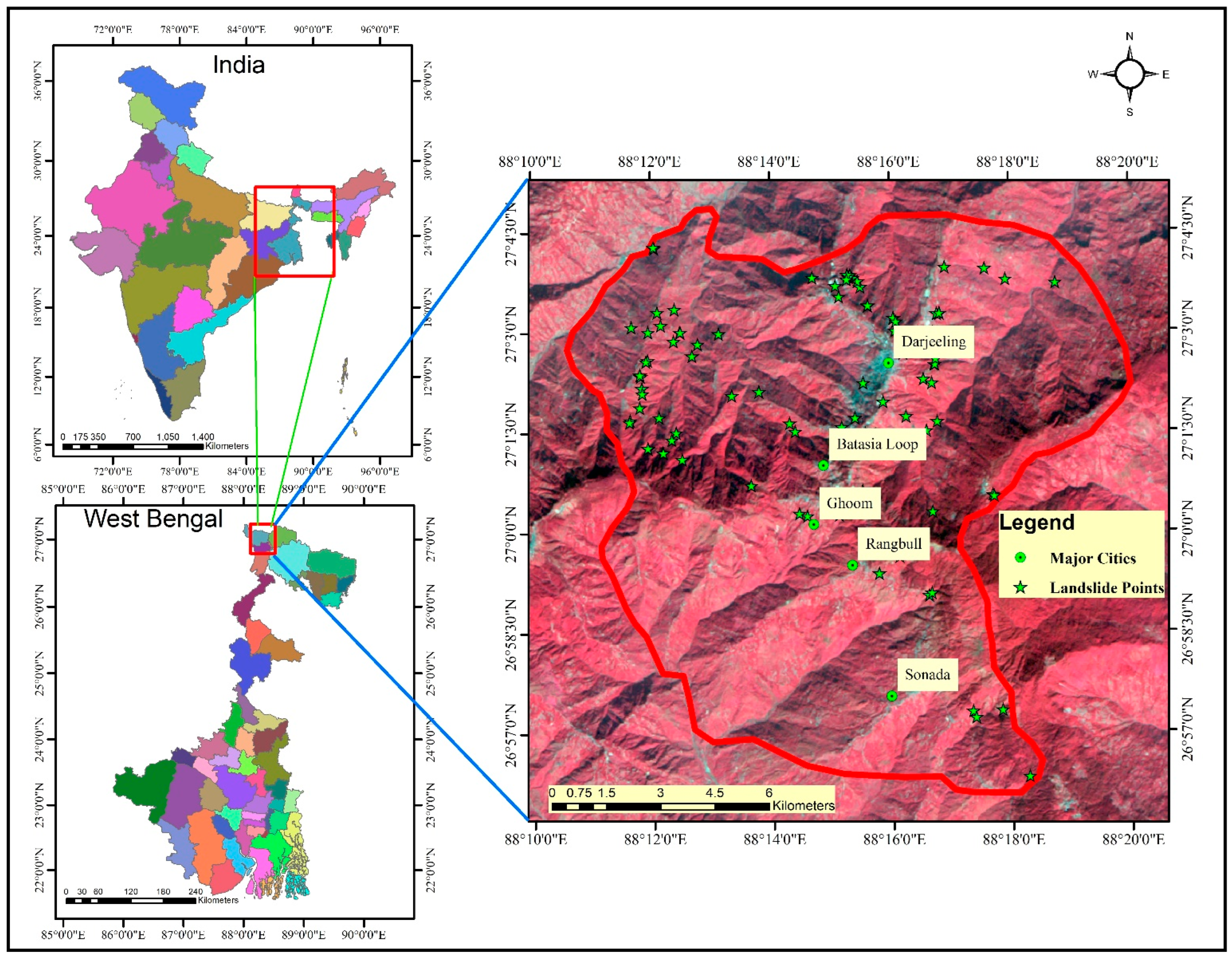
2.1. Study Area

The Eastern Himalayan region, specifically the district of Darjeeling and Kurseong, is where our study area is located in India (Figure 1). The research area is located between longitudes 88°2′51″ E and 88°5′42.6″ E and latitudes 26°15′33″ N to 27°1′22″ N. In this region, both plain and mountainous topographies have their features. The total area covered in the study area is 165.92 sq.km. The region’s altitude is between 15 and 2584 m above mean sea level [24]. The Lesser and Sub-Himalayan belts include the Darjeeling Himalayas. The stratigraphic superposition of the tectonic units in the region is reversed. Numerous rock groups have received local recognition [25]. Different geomorphological structures, such as steep slopes and dissected hills with valleys, are present in this region. Due to the mountainous terrain, Darjeeling’s average yearly temperature is almost 14.9 °C; however, during the winter, it drops to almost 1 °C. The current record-low temperature is −5 °C. Every year, from the middle of April to the end of August, there is huge rainfall because of the region’s low-temperature climate. In the study area, the average rainfall is 2074.08 mm. The important cities in this region include Kurseong, Darjeeling, Ghum, and Sonada. The most land-intensive characteristic is the tea plantation and horticulture. Darjeeling is well-known for its tea, mountains, and tourism. Every year, 50,000 tourists worldwide and nearly 500,000 visitors from India visit Darjeeling, Kurseong, and its surroundings. Nearly 12,000 people per square km make up the population. The graphical representation of overall methodology is in Figure 2.

2.2. Data Sources

In this study, various data sources were used to generate different kinds of data (

Table 1. Different data sources.

Sl. No	Input Data	Spatial Resolution	Resultant Maps
1	ALOS PALSAR DEM	12.5 m	Slope, aspect, profile curvature, drainage density, lineament density
2	Cartosat-2 series (MX)	1.6 m	Land use and land cover
4	CRU data	Numerical	Rainfall
5	Geomorphology, lithology	--	Geomorphology, lithology
6	Soil	--	Soil texture

). These data come from historical records (data reports from the Geological Survey of India) and field research. High-resolution satellite imagery, such as Cartosat-2D (multi-spectral) with a spatial resolution of about 1.6 m, Advanced Land Observing Satellite-1 (ALOS) Phased Array type L-band Synthetic Aperture Radar (PALSAR) digital elevation model (DEM) with 12.5 m spatial resolution, and Advanced Spaceborne Thermal Emission and Reflection Radiometer (ASTER) DEM data of 30 m resolution. Rainfall data were collected from the Current Research Unit (CRU). Soil data collected from International Satellite Land Surface Climatology Project (ISLSCP) (http://www.gewex.org/is-lscp.html (accessed on 31 May 2022)) Initiative II Data Collection, and geomorphology and lithology data were gathered from the BHUKOSH website (https://www.bhukosh.gsi.gov.in (accessed on 31 May 2022)) for the Government of India.

2.3. Landslide Inventory Map

When creating the landslide susceptibility maps, it is crucial to accurately pinpoint the landslide’s position and extent. An essential component and core piece of information for any landslide zoning, including susceptibility, risk, and hazard zonings, is the landslide inventory. It relates to the location, type, amount, travel distance, the intensity of activity, and date of an area’s land sliding [26]. There are numerous ways to recognize landslides. Aerial photographs, satellite views, a literature review for the information on previous landslides, and field observations are among them [16]. Field data, visual interpretation of aerial photos, and satellite imagery were used to create the landslide inventory map [17]. The Geological Survey of India published detailed landslide inventory data for India. The inventory map of the study area was resampled and incorporated in the study from the published data of the geological Survey of India. The published data has been used in this study to identify 114 landslides (Figure 3a). The bulk of landslides that have been reported in this area have happened on cliffs, banks, and highways. Cliffside landslides are frequently caused by erosion, steep slope topography, and loss of vegetation.

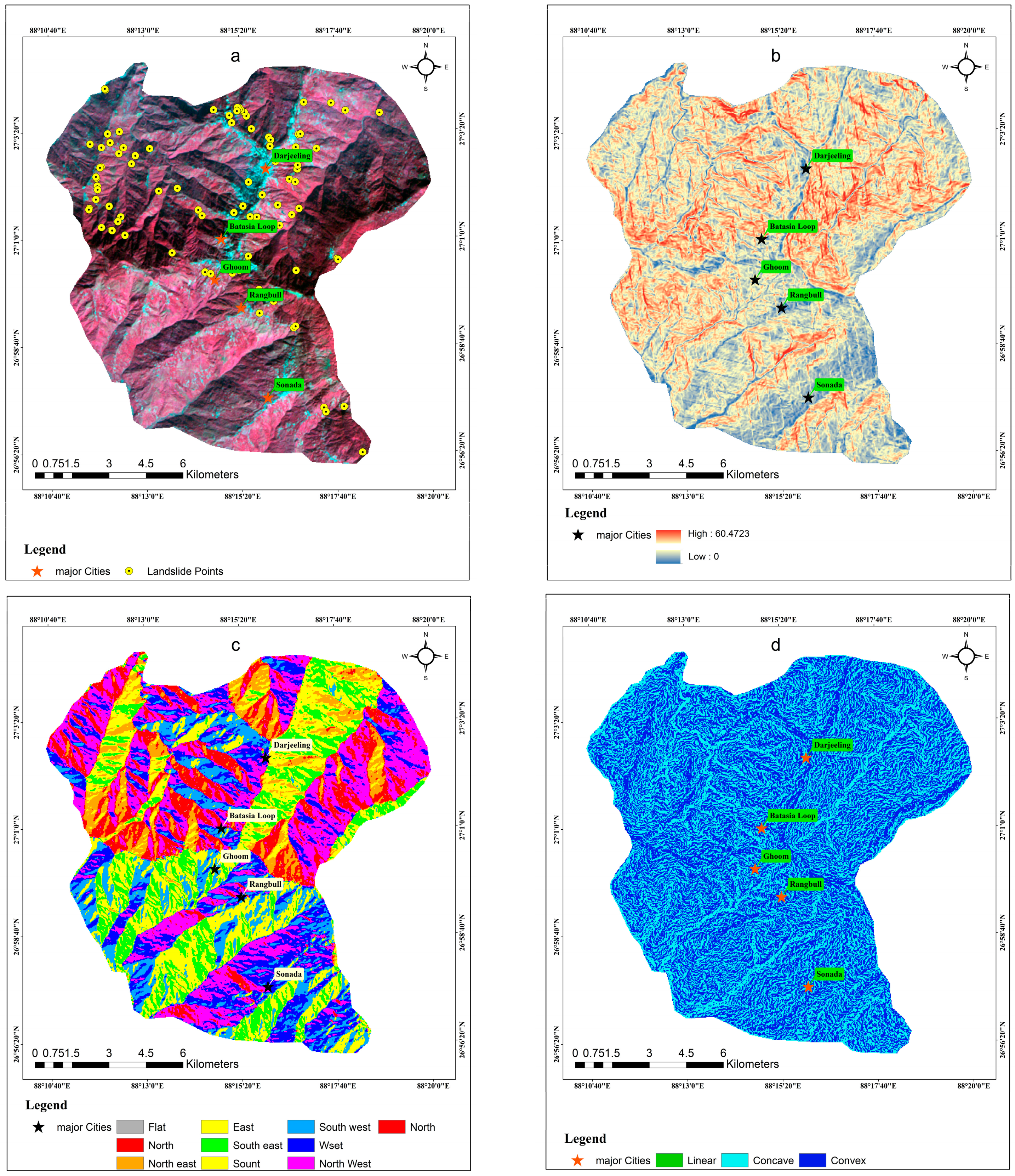
2.4. Landslide Conditioning Factors

2.4.1. Slope

The slope is a crucial factor in the examination of any area’s potential for a landslides. Hilly terrain and steep slopes characterize the study region. That explains why the basin has a lot of slopes throughout. The slope was classified into five classes in the study area: very high, high, moderate, low, and very low slope. There are very few areas in the study area with very low slopes (<15°) (Figure 3b). Low slope class is between the slope angle range of 15° to 25°. High and very high slopes were defined as from 35° to 45° and greater than 45°, respectively. Landslides frequently occur where the degree of slope is high; hence, high and very high slope places are more likely to experience landslides. Conversely, locations with a moderate to low slope are more or less stable when it comes to landslide incidence [27].

2.4.2. Aspect

An essential factor in determining landslide vulnerability is the slope direction aspect. With a latitude range of 26°15′33″ N to 27°01′22″ N, the research region is located in the northern hemisphere, where rainfall and sunshine intensity are quite high for slopes that point south, east, or west, respectively [28]. The slope orientation toward the south is encountering the most inputs among them. Because slope direction towards the north receives the least impetus in terms of the specified criteria, its susceptibility is the lowest, while slope direction towards the south is the highest [29]. The rest of them are only mildly impacted. A significant portion of the research area is located on the slope facing east and south. The lowest portion of this basin is covered by a slope angle facing west, while a slope facing north covers a moderate to low slope area (Figure 3c).

2.4.3. Profile Curvature

Profile curvature is an important topographic feature for landslides (Figure 3d) [30,31]. The moistness holding capacity of soil is determined by its concavity (negative curvature) or convexity (positive curvature). The curvature value represents the topography’s morphology. A positive curvature value at the pixel denotes an upwards convex surface, a negative curvature value denotes an upwardly concave surface, and a value of 0 denotes a flat surface. Positive curvature values correspond to convex slopes, while negative curvature values correspond to concave slopes [32]. Drainage density, slope saturation, and slope instability are all introduced by a slope segment with a higher positive or negative curvature value. A concave slope collects extra water and completely drenches the soil, which weakens the cohesiveness of the soil [33]. On the other hand, a convex slope is more vulnerable to numerous cycles of contraction and expansion, which leads to rock breakdown and dissolution. Water can percolate through loosening or decomposed materials on a convex slope, causing pore water pressure to rise and slope instability.

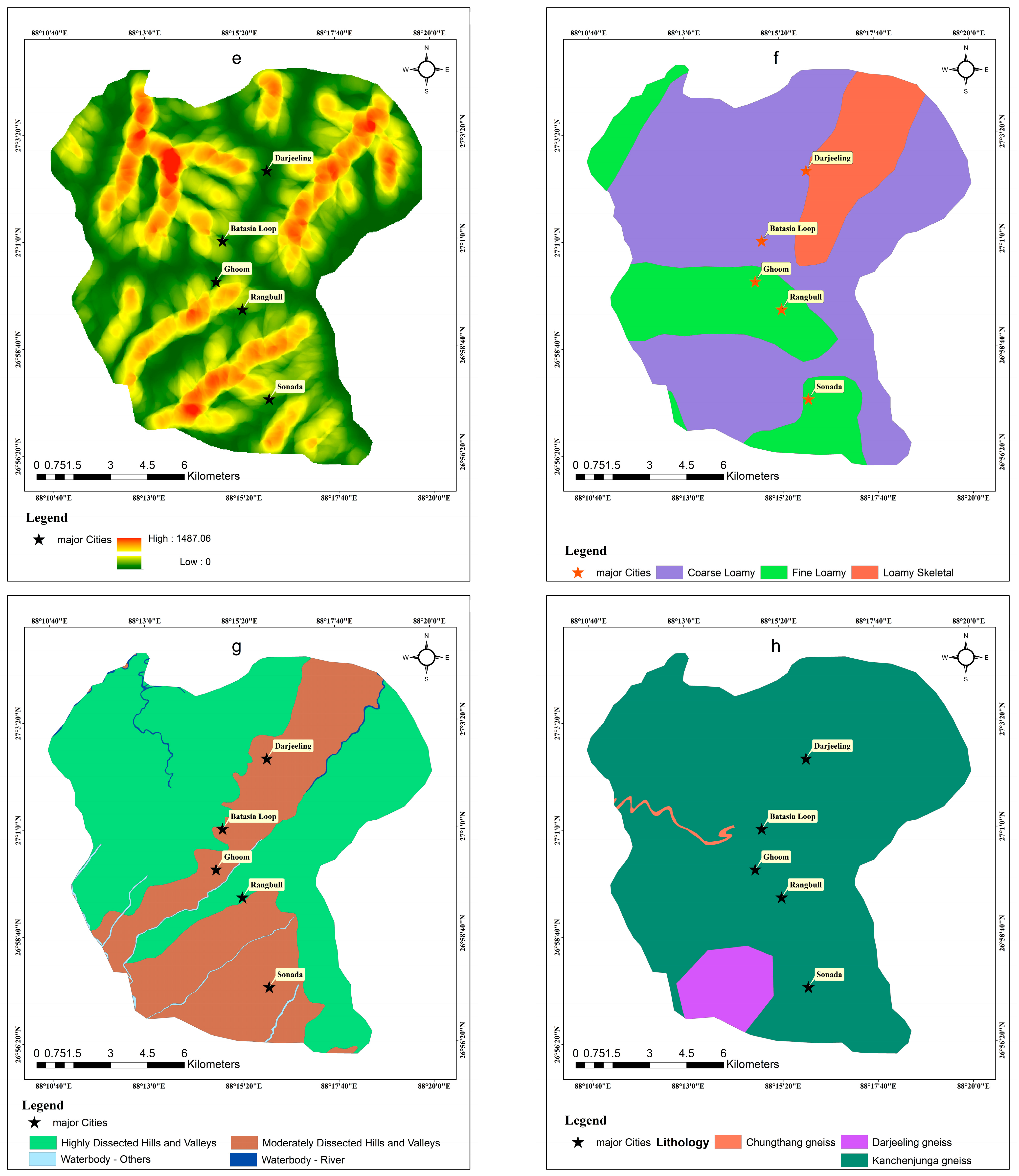
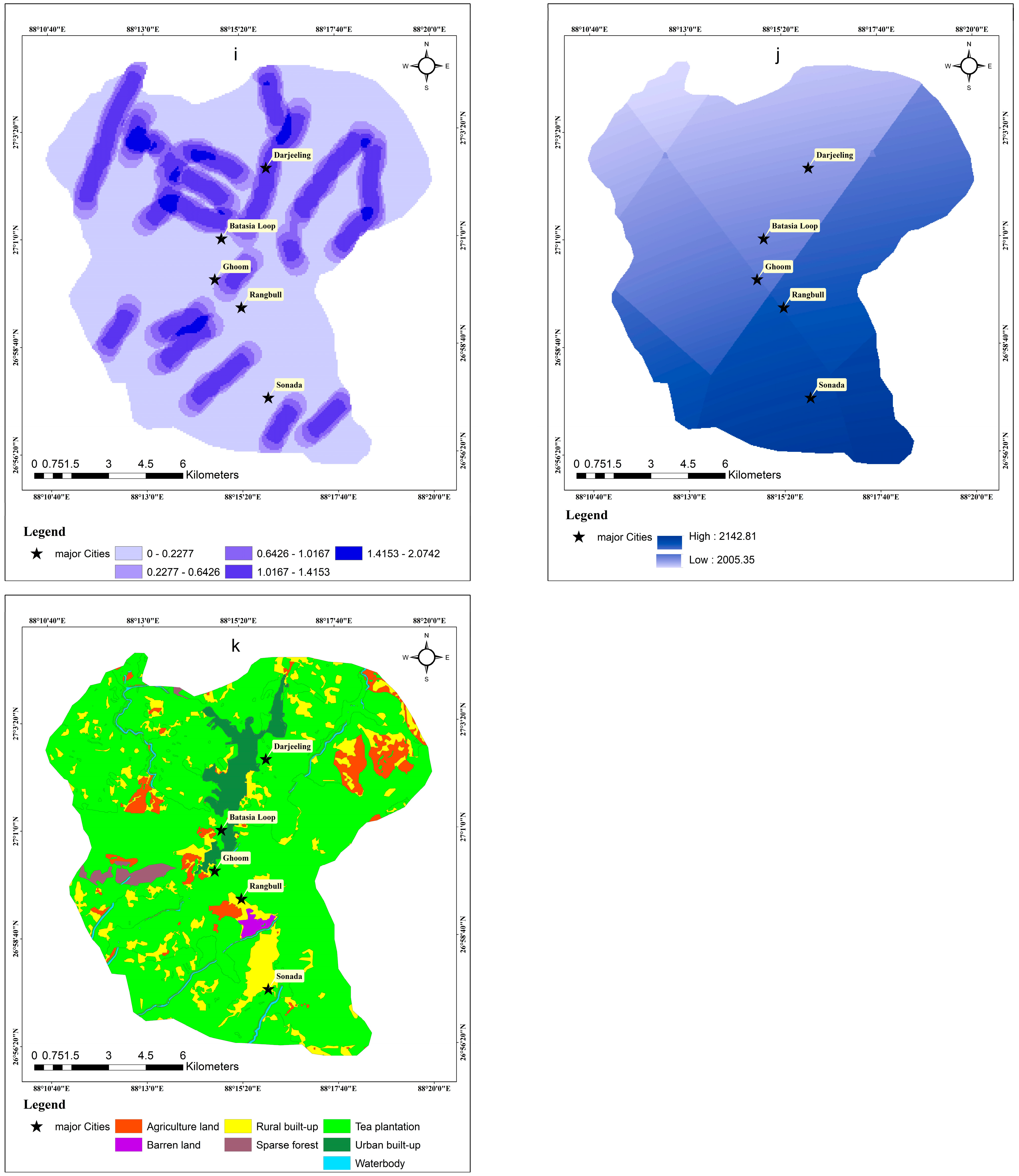
2.4.4. Drainage Density

The length of streams per unit area in a drainage basin is what Mandal and Mondal (2019) refer to as drainage density (Figure 3e) [34]. Due to soaking up the water, the material comes close to the slope base; hence, degradation of slope stability happens [35]. The amount of drainage density determines how much landslides affect streams. The following Equation (1) was used to determine the drainage density:

$$\mathrm{Drainage}\mathrm{density}=\frac{\mathrm{Len}}{\mathrm{S}}$$

(1)

where Len is the overall measurement of the drainage system and S is the size of the drainage basin. Drainage density maps were created using the Euclidean distance approach, and in a GIS context, they were divided into five categories: 0–150 m, 150–250 m, 250–350 m, 350–450 m, and >450 m.

2.4.5. Soil Texture

The International Satellite Land Surface Climatology Project (ISLSCP) Initiative II Data Collection (http://www.gewex.org/is-lscp.html (accessed on 31 May 2022)) is a second non-satellite database that offers gridded data for 18 chosen soil parameters. The Oak Ridge National Laboratory Distributed Active Archive Center (http://daac.ornl.gov/ (accessed on 31 May 2022)) provides these data sets with a quarter-degree resolution. The soil texture (Figure 3f) is a crucial factor in this investigation. Coarse loamy soil, loamy skeletal, and fine loams are three different textural groups.

2.4.6. Geomorphology

Geomorphology is a significant component in landslide susceptibility assessment. The Government of India collected geomorphological maps from the website called BHUKOSH (https://www.bhukosh.gsi.gov.in (accessed on 31 May 2022)). A significant percentage of the area’s structural origin is linked to the region’s extensively dissected hills and valleys. It can be identified by its steep slope, the existence of an escarpment, and a noticeable cliff [36]. The lower portion of the study area contains a structural origin of moderately dissected hills and valleys, which is a different type of geomorphology (Figure 3g). Valleys with steep to moderate slopes and valleys with moderate to steep slopes set this region apart. Waterbodies (river) and waterbodies (others) cover the remaining area.

2.4.7. Lithology

The composition and structure of various lithologies are responsible for the rock’s strength [16]. Stronger rocks are less susceptible to landslides than weaker rocks because they provide more resistance to driving forces. The opposite is also true. The co-registered geological map of the Sikkim-Darjeeling area’s polygons were digitally converted into a vector layer to create the lithology data layer. After field verification, necessary adjustments have also been included in this vector layer. Later, a 30 m spatial resolution rasterization of this lithology data layer was performed (Figure 3h). This data layer contains three lithological types: Darjeeling gneiss, Chungthang gneiss, and Kanchenjunga gneiss.

2.4.8. Lineament Density

Lineaments are structural characteristics that identify unstable zones or planes, fractures, and faults along which landslides are more likely to occur. It has typically been shown that lineaments, which alter both the surface material structures and the terrain’s permeability, which contributes to slope instability, enhance the likelihood of landslides occurring at sites nearby [37]. ALOS PALSAR DEM pictures have been used to interpret lineaments. Tonal contrast, structural alignments, rectilinear tendencies of morphological features, and linear stream courses that are remarkable for abrupt changes in course were used to interpret the lineaments. Although massive lineaments have been found, the research region has not been reported to contain any significant thrusts or faults. The lineament data layer was created by rasterizing the interpreted lineaments after they had been digitally captured on-screen. The lineament density map (Figure 3i) was created using the lineament data layer as a reference and divided into five groups using the natural break algorithm.

2.4.9. Rainfall

One of the main initiating factors for landslide occurrences in the study area is rainfall (Figure 3j). Rainfall results in unexpected floods and small landslides [38]. Due to severe rainfall, water infiltrates quickly and increases saturation level. It is an external temporal triggering element, and too much of it can produce downhill slides by making the slope heavier by raising the pressure of the pore water [16]. The Thiessen Polygon method created a rainfall distribution map from Climate Research Unit (CRU) datasets. It was then classified into five categories using the natural breaks algorithm, which resulted in the following range: 2005.35–2032.85 mm, 2032.85–2060.34 mm, 2060.34–2087.83 mm, 2087.83–2115.32 mm, and 2115.32–2142.81 mm, as this method minimizes the variance of data range within a class and maximizes the difference between classes.

2.4.10. Land Use and Land Cover

Land use and land cover (LULC) is an indirect measure of slope strength because it controls the rate of weathering and erosion. It is one of the primary factors influencing the occurrence of landslides in hilly areas. The LULC map (Figure 3k) was created in this study using the CARTOSAT-2 series (MX) image. The interpreted LULC was digitized and then rasterized on a 30 m × 30 m pixel size. The LULC map is divided into various classes, such as agriculture land, barren land, rural area, urban area, sparse forest, tea plantation, and waterbody. The majority of the basin is covered in forest; agricultural land and developed areas with good road connectivity can be found in the southern part of the area. Human interference is prevalent in the southern region but less so in the northern region due to inaccessibility.

2.5. Models Used for Landslide Susceptibility Mapping

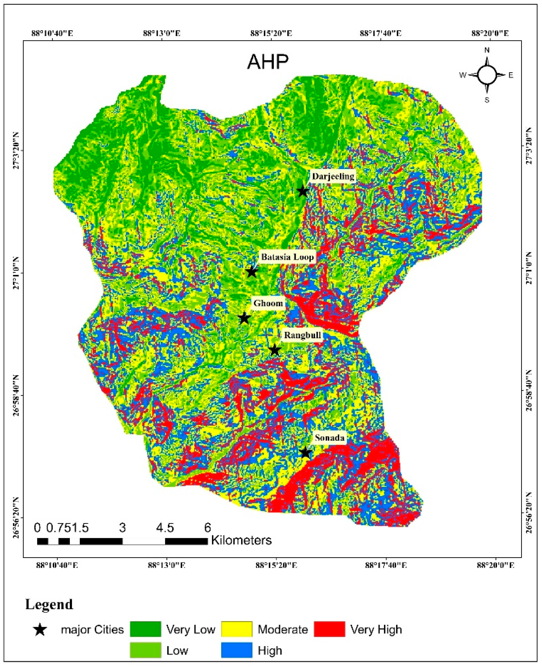
2.5.1. Analytical Hierarchy Process (AHP)

An organized way for analyzing and evaluating complicated decisions based on mathematics is the multi-criteria decision analysis (MCDA) method, sometimes known as the AHP. To create the susceptibility map, the elements impacting susceptibility must be incorporated. Based on their significance, the layers have been given different weights. The pairwise comparison method is utilized in AHP for decision-making frameworks that consider numerous factors. The AHP approach is used to conduct both qualitative (subjective) and quantitative (objective) decision-making analyses [39]. The comparison matrix is made up of an equal number of rows and columns, with the diagonal of the matrix having the value 1 and one side of it housing the scores. To create a pairwise confusion matrix, each layer’s performance should be compared with that of other layers. The rating value falls between 1 and 9. The relevance of the two elements is represented by each pairwise comparison matrix value. It was considered that if attribute A is ranked at 9 and is more significant than attribute B, then B must be rated at 1 and is less significant than A. λ_max equals the products between each component of the priority vector and the column totals, where λ_max is the major eigenvalue and n is the number of elements.

To validate a pairwise comparison matrix, consistency index (CI) and consistency ratio (CR) calculations are required [40,41,42]. We need to know the value of the proposed random consistency index (RI) (

Table 2. The random consistency index value for AHP [42].

NO.	1	2	3	4	5	6	7	8	9	10
RI	0	0	0.58	0.90	1.12	1.24	1.32	1.42	1.45	1.49

) in order to calculate the CR [43]. We can accept the pairwise comparison matrix if the value of CR is less than 0.10. CI and CR are computed using the following formula [42]:

$$\mathrm{CI}=\frac{{\mathsf{\lambda }}_{\max }-\mathrm{n}}{n-1}$$

(2)

$$\mathrm{CR}=\frac{\mathrm{CI}}{\mathrm{Random}\mathrm{Consistency}\mathrm{Index}\left(\mathrm{RI}\right)}$$

(3)

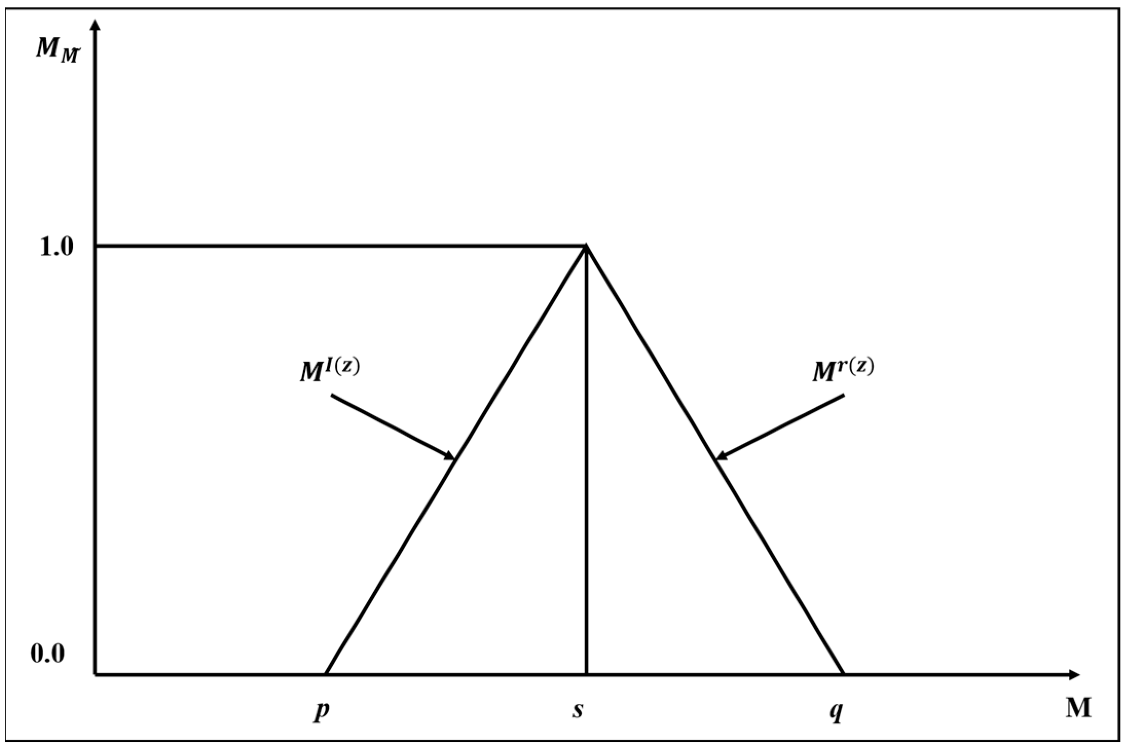
2.5.2. Fuzzy-Based Analytical Hierarchy Process (Fuzzy-AHP)

The fuzzy set theory modeling approach was first developed by Zadeh (1965) [44]. It replicates complicated systems that are challenging to understand in terms of specific numbers. Information that is ambiguous, imprecise, and hazy can be input using fuzzy logic [45]. The spatial item on a map is typically implemented as a fuzzy membership function in decision-making. The degree of the membership function is demonstrated by fuzzy set theory, which allows the possibility of objects belonging as a membership value that varies between 0 and 1 [46]. A triangular fuzzy member (TFM) M͂ is illustrated in Figure 4.

When written as (p/s, s/q) or (p, s, q), a triangular fuzzy number (TFN) denotes the smallest, most likely, and most significant values, respectively. The TFN with sequential representation on the left and right side can be referred to as, in terms of its membership function:

$$\mu \left(y/\tilde{\mathrm{M}}\right)=\left\{\begin{array}{cc}0,& y<p,\\ \left(y-p\right)/\left(s-p\right),& p\le y\le s\\ \left(q-y\right)/\left(q-s\right),& s\le y\le q\\ 0,& y>q\end{array}\right\}$$

(4)

As seen below, a fuzzy number has a left and right representation for each degree of membership [47].

$$\tilde{M}=\left(M^{l\left(z\right)},M^{r\left(z\right)}\right)=\left(p+s-p\right)z,q+\left(s-q\right)z)$$

(5)

where the terms l(y) denote the left side of fuzzy members, and l(r) represents the right side of a fuzzy number.

In order to effectively describe ambiguous data, fuzzy membership functions (FMFs) and fuzzy set theory are essential. Additionally, it permits the application of mathematical and programming operations in the fuzzy domain. A class of objects known as a fuzzy set is one in which each item is assigned a membership grade between 0 and 1, and vice versa, using a membership function [44]. Because of fuzzy sets theory, partial membership of an investigated site for more than one susceptibility class is theoretically feasible in the context of landslide susceptibility mapping. This analysis of the geographical diversity and its pattern, which resulted in the creation of continuous class boundaries for each hazard zone, was undertaken using FMFs. The form of each applied FMF determines when the transition between 0 and 1 occurs.

Since the traditional AHP cannot fully describe the decision-making process based on quantitative preference articulation, a fuzzy extension of AHP (known as fuzzy-AHP) was created to tackle the fuzzy hierarchical challenges. The fuzzy-AHP approach was used for fuzzy-weight hierarchical analysis in the current study by allocating fuzzy numbers for pairwise comparisons. The following steps were performed to establish evaluation criteria using fuzzy-AHP weights [48]:

Step I: Using each of the components/criteria in the hierarchy system’s dimensions, pairwise comparison matrices were created. In order to determine which of the two aspects or criteria was more crucial in each situation, the following linguistic phrases were applied to the pairwise comparisons:

$$\tilde{A}=\left[\begin{array}{cccc}\tilde{1}& {\tilde{a}}_{12}& \cdots & {\tilde{a}}_{1n}\\ {\tilde{a}}_{21}& \tilde{1}& \dots & {\tilde{a}}_{2n}\\ ⋮& ⋮& \ddots & ⋮\\ {\tilde{a}}_{n1}& {\tilde{a}}_{n2}& \cdots & \tilde{1}\end{array}\right]=\left[\begin{array}{cccc}\tilde{1}& {\tilde{a}}_{12}& \cdots & {\tilde{a}}_{1n}\\ \raisebox{1ex}{$1$}\!\left/ \!\raisebox{-1ex}{${\tilde{a}}_{21}$}\right.& \tilde{1}& \dots & {\tilde{a}}_{2n}\\ ⋮& ⋮& \ddots & ⋮\\ \raisebox{1ex}{$1$}\!\left/ \!\raisebox{-1ex}{${\tilde{a}}_{n1}$}\right.& \raisebox{1ex}{$1$}\!\left/ \!\raisebox{-1ex}{${\tilde{a}}_{n2}$}\right.& \cdots & \tilde{1}\end{array}\right]$$

(6)

where ã_ij is, when $\tilde{1}$ be (1,1,1), if i = j; if $\tilde{1},\tilde{2},\tilde{3},\tilde{4},\tilde{5},\tilde{6},\tilde{7},\tilde{8},\tilde{9}$ measure that is when i is relatively important to j and if j is relatively important to i then $\tilde{1}-1,\tilde{2}-1,\tilde{3}-1,\tilde{4}-1,\tilde{5}-1,\tilde{6}-1,\tilde{7}-1,\tilde{8}-1,\tilde{9}-1$ is measured (

Table 3. AHP to fuzzy-AHP weight conversion table.

Scale Weight	Triangular Fuzzy Scale	Scale Weight	Triangular Fuzzy Scale
1	(1,1,1)	1/1	(1/1, 1/1, 1/1)
2	(1,2,3)	1/2	(1/3, 1/2,1/1)
3	(2,3,4)	1/3	(1/4,1/3,1/2)
4	(3,4,5)	1/4	(1/5,1/4,1/3)
5	(4,5,6)	1/5	(1/6,1/5,1/4)
6	(5,6,7)	1/6	(1/7,1/6,1/5)
7	(6,7,8)	1/7	(1/8,1/7,1/6)
8	(7,8,9)	1/8	(1/9,1/8,1/7)
9	(9,9,9)	1/9	(1/9, 1/9, 1/9)

).

Step II: Using Buckley’s (1985) fuzzy geometric mean and fuzzy weights for each criterion, define them as follows using the geometric mean technique [49]:

$${\tilde{r}}_i={\left({\tilde{a}}_{i1}\otimes {\tilde{a}}_{i2}\otimes \dots \otimes {\tilde{a}}_{in}\right)}^{\raisebox{1ex}{$1$}\!\left/ \!\raisebox{-1ex}{$n$}\right.}$$

Then,

$${\tilde{w}}_i={\tilde{r}}_i\otimes {\left({\tilde{r}}_i\otimes \dots \otimes {\tilde{r}}_i\right)}^{-1}$$

(7)

where ã_in is the fuzzy comparison value between criteria i and criterion n, ${\tilde{r}}_i$ is the geometric mean of this fuzzy comparison value, and ${\tilde{w}}_i$ i is the fuzzy weight of the ith criterion, which a TFN can represent, with $\tilde{w}$ = (p_wi, s_wi, q_wi). Here, p_wi, s_wi, and q_wi denote the lower, middle, and upper values, respectively, of the fuzzy weight of the ith criterion.

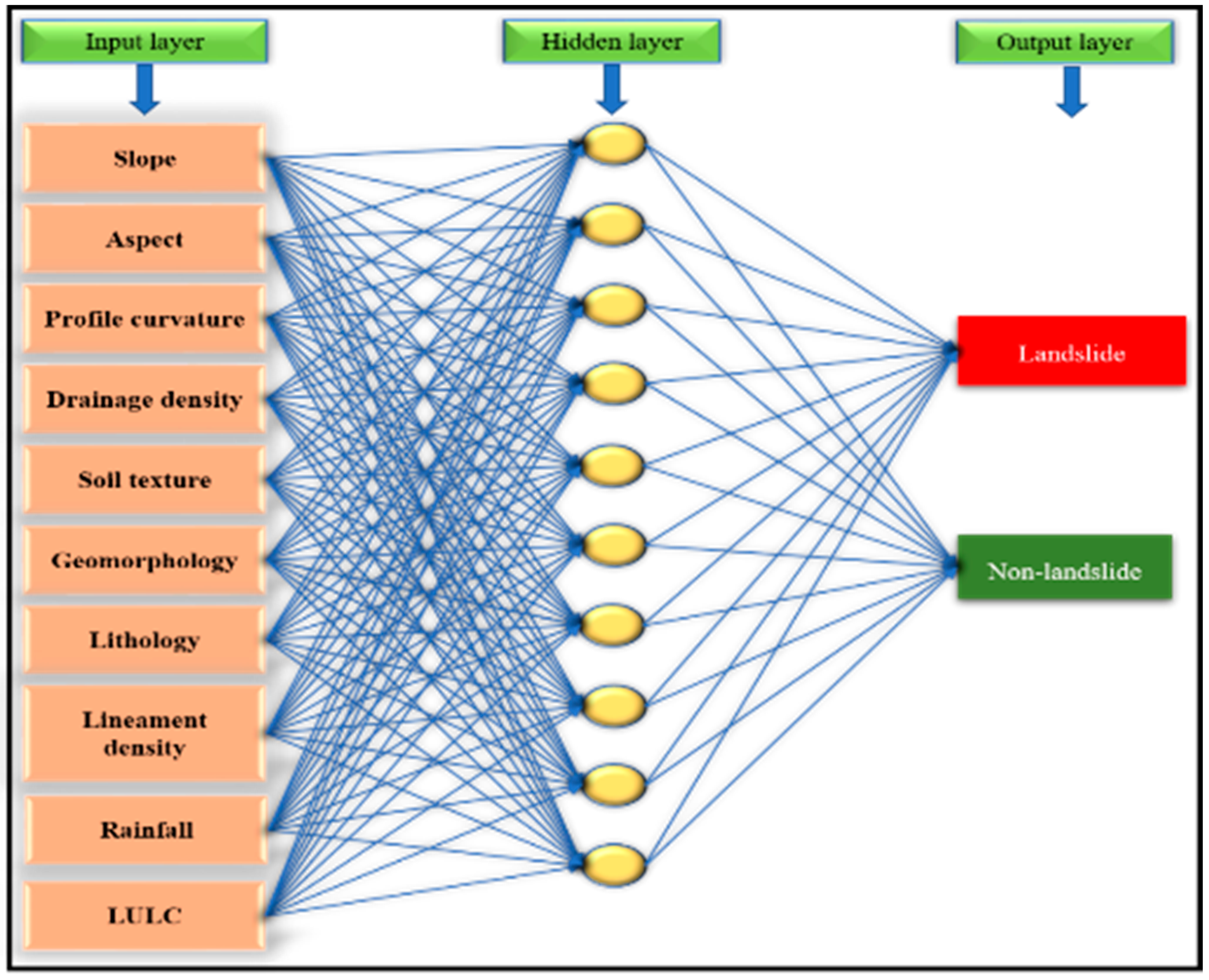
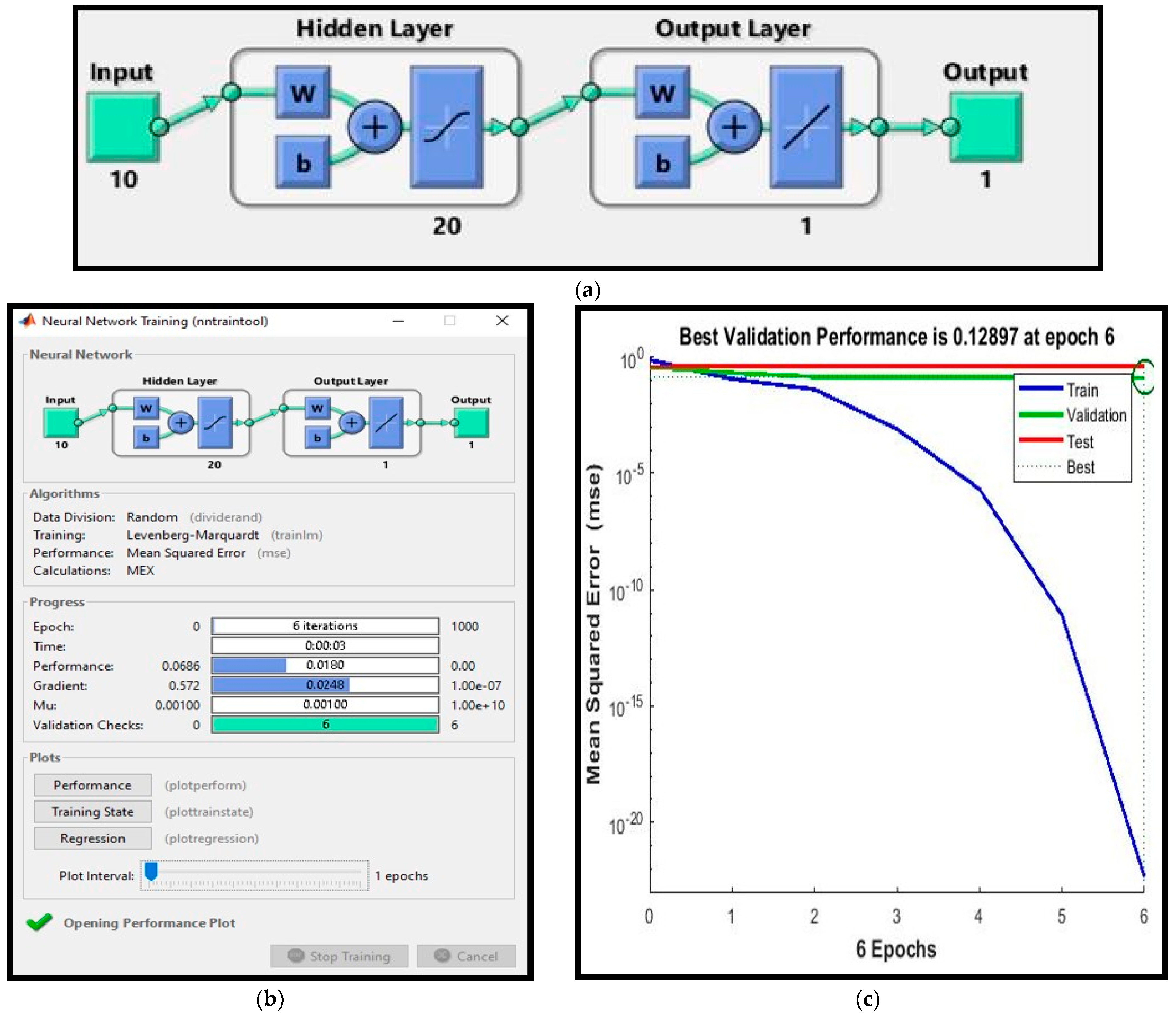
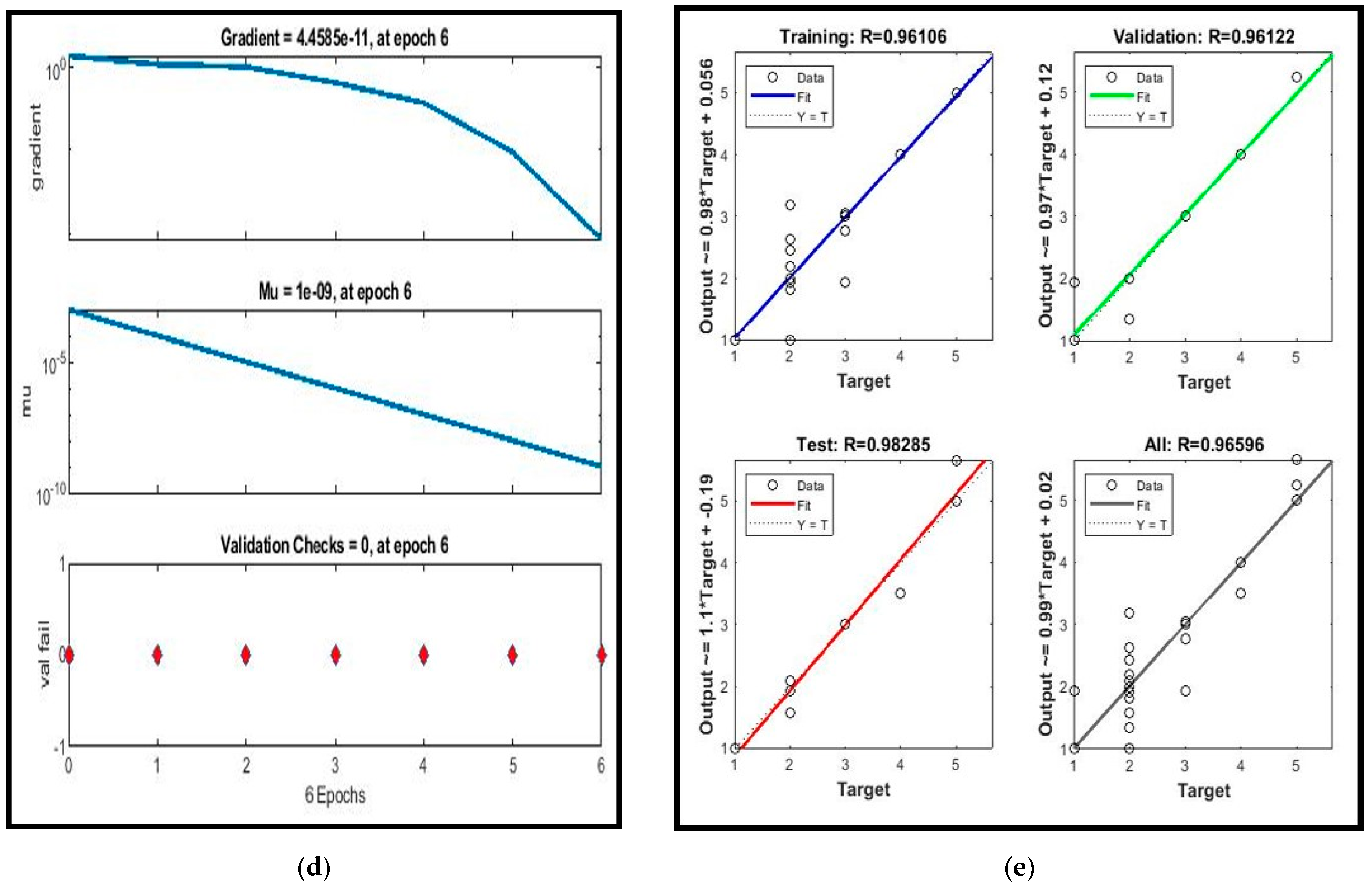
2.5.3. Artificial Neural Network (ANN)

As a general nonlinear function approximation algorithm, artificial neural networks (ANNs) are used in machine learning (ML) to generate new knowledge by evaluating and interpreting data relationships [50]. It is an advanced network of neurons that analyses data based on connecting weight and outputs of the results to the layer below [51]. The process of continuously modifying the network parameters is the ANN model’s learning process. All the layers are positioned adjacent to one another and connected by the defined weight traveling from layer to layer. Next, the weights for each of the next layers will be established [51]. Additionally, even when the interactions between the input parts are hazy or hard to express physically, the ANN model may nevertheless forecast using the input data [34]. As a result, the ANN model is a useful tool in the context of landslides and is frequently used to map landslide risk.

The input layer, hidden layer, and output layer are the three parts of an ANN. The landslide conditioning factors chosen for the model development are considered when building the input layers. Each landslide conditioning element connecting the input layer to the hidden layers has its own neuron. Unnoticed classifier elements responsible for processing and changing data from input to output are known as hidden layers. Multiple neurons contributed to the complexity of the input neurons from hidden levels. A landslide or non-landslide area was classified in this study using the output layer’s single neuron that correlated to the final output. Figure 5 depicts the model structure. Back-propagation algorithms, which are often employed by landslide researchers [52], were applied in this study. A back-propagation approach is utilized to calculate the weights used in the network by calculating a gradient [25].

Based on the significance of landslide conditioning factors, a map of landslide susceptibility was created. The weighted value for each landslide conditioning element was calculated after a successful network training. The normalized ranges between 0 and 1 were used to determine each and every one of the weighted landslide conditioning factors. Five susceptibility levels are now shown on the map: very low susceptibility, low susceptibility, moderate susceptibility, high susceptibility, and very high susceptibility. The classification approach is the natural break strategy [53,54].

2.5.4. Parameter Effectiveness of the Model

The degree of multicollinearity is measured using the variance inflation factor (VIF) in least squares regression analysis. The exponent represents the increase in coefficient estimated via multicollinearity [55]. The amount of multicollinearity may be estimated from the size of the VIF. According to an experimental rule, multicollinearity is high if the VIF value is more than 5. The tolerance margin of error is the second method for examining multicollinearity (T). A relatively general type of multiple correlation coefficient is tolerance [56]. A variable with zero margins of error is fully multicollinear since it is entirely foreseeable from other independent variables. It is evident that a variable is totally uncorrelated with the other independent variables if its tolerance value equals 1 [57]. The study was found to be multicollinear using the criteria VIF and T. Tolerance and VIF were computed using the following formulas:

$$\mathrm{Tolerance}=1-{\mathrm{R}}_{\mathrm{j}}{}^2$$

(8)

$$\mathrm{VIF}=\frac{1}{\mathrm{Tolerance}}$$

(9)

Here, R_j² is the correlation coefficient (R-squared) of the model to the descriptive variable j.

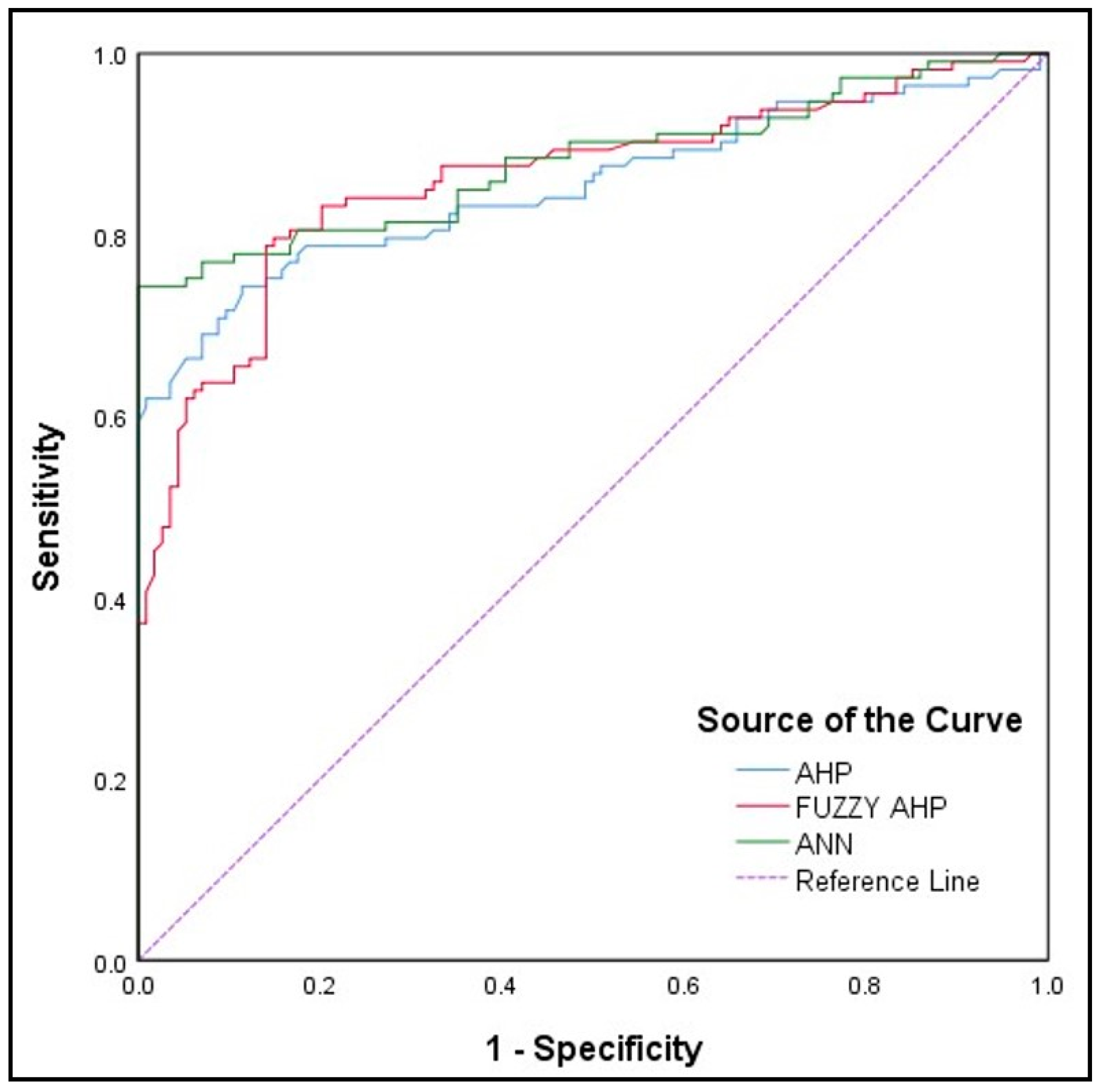
2.5.5. Performance Evaluation of the Model

The effectiveness of landslide susceptibility models can be assessed using a variety of statistical metrics. Several validation model evaluation methodologies, such as sensitivity, receiver operating characteristics (ROC), specificity, area under curve (AUC), and accuracy, were used in this work to validate the performance of the prediction model. The effectiveness of landslide prediction has recently been extensively assessed using the ROC curves method [58,59]. The inputs used to plot the ROC curve were true positive, which stands for a properly anticipated landslide on the X-axis, and false positive, which stands for an incorrectly predicted landslide on the Y-axis. AUC, a statistical evaluation of the inclusive effectiveness of the models, was employed for quantitative comparison. AUC and prediction model accuracy are graded as weak when the value is between 0.5–0.6, moderate when the value is between 0.6–0.7, good when it is between 0.7–0.8, and outstanding when it has a quantitative value between 0.8 to 0.9 [60]. As a result, AUC values can be used as a benchmark when evaluating the precision of a prediction model.

The definition of a detection method’s sensitivity is the percentage of landslide sites that are correctly categorized as landslide occurrence, while the definition of specificity is the percentage of non-landslide locations that are reliably labeled as non-landslide occurrence [61,62]. Additionally, accuracy evaluates the percentage of correctly identified non-landslide and landslide locations. These statistical measures were computed in this investigation using Equations (10)–(12) [63] as follows:

$$\mathrm{Specificity}=\frac{\mathrm{TN}}{\mathrm{TN}+\mathrm{FP}}$$

(10)

$$\mathrm{Sensitivity}=\frac{\mathrm{TP}}{\mathrm{TP}+\mathrm{FN}}$$

(11)

$$\mathrm{Accuracy}=\frac{\mathrm{TP}+\mathrm{TN}}{\mathrm{TP}+\mathrm{TN}+\mathrm{FP}+\mathrm{FN}}$$

(12)

where the number of points correctly labeled as landslides is known as true positive (TP), the number of points correctly classified as non-landslide points is known as true negative (TN). The amount of landslide points that were mistakenly identified as non-landslide or landslide sites are referred to as false positive (FP) and false negative (FN).

3. Results

3.1. Multicollinearity Test and Correlation Results

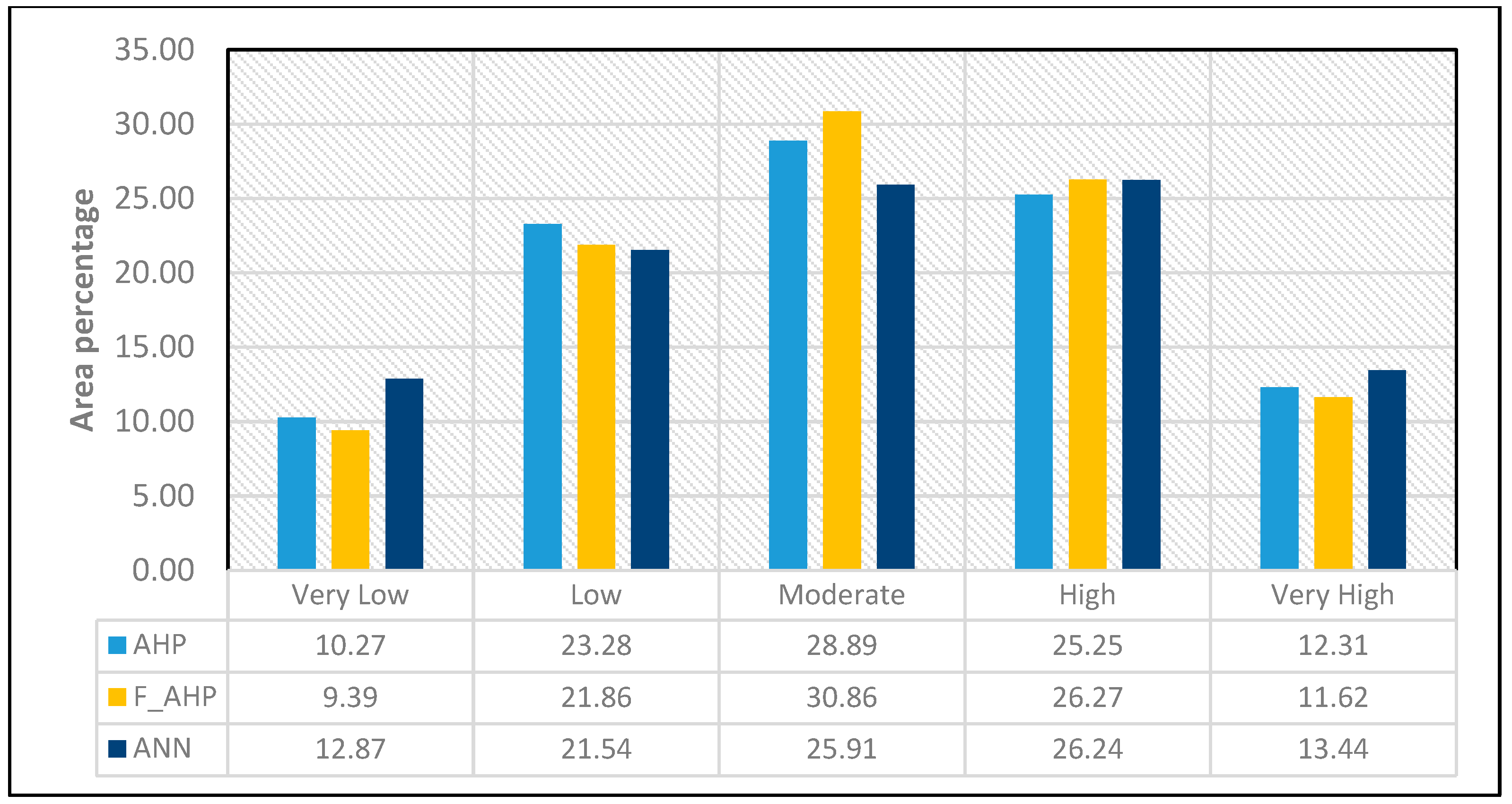
When choosing the conditioning factors based on the non-independence of the factors, the underlying assumption can be examined to see if it is appropriate using a multicollinearity analysis. To identify and measure multicollinearity among the ten landslide conditioning factors, VIF and T were put into use. Only minor multicollinearity among the chosen independent variables is shown by tolerance values of less than 0.2, while multicollinearity is strongly suggested by tolerance values of less than 0.1 [64]. According to the findings, the highest VIF value was 1.342, and the lowest tolerance value was 1.043. The critical thresholds for the multicollinearity assessment among the ten conditioning factors were met because all of the VIF values fell below the theoretical critical value (5 or 10). Each and every tolerance value exceeded the theoretical threshold level (0.1 and 0.2). The minimum and maximum tolerance values were 0.745 and 0.959, respectively, whereas the highest and lowest VIF values, which correspond to aspect and profile curvature, were 1.342 and 1.043. As a result, there is no multicollinearity between any of the chosen conditioning components (

Table 4. The multicollinearity analysis for landslide conditioning factors.

Sl. No	Class	Tolerance	VIF
1	Soil texture	0.857	1.167
2	Slope	0.874	1.144
3	Rainfall	0.797	1.255
4	Profile Curvature	0.959	1.043
5	Land use and land cover	0.843	1.186
6	Lithology	0.944	1.060
7	Lineament Density	0.869	1.151
8	Geomorphology	0.816	1.225
9	Drainage Density	0.922	1.085
10	Aspect	0.745	1.342

).

3.2. Model Results

In the present work, three different models were applied to generate a landslide susceptibility map.

3.2.1. Assessment Using AHP Model

Each causative factor was given a weight before the weighted linear combination sum technique was used to build a landslide susceptibility map [65]. The landslide susceptibility map for the research region (Figure 6) indicated a tolerable CR of 0.0963 (less than 0.1), with slope, rainfall, profile curvature, LULC, and soil as key factors. To rank each class, the frequency ratio value between pixels damaged by the landslide and unaffected pixels was employed. Based on the ranking values, class weights for each class of landslide causative factors were determined using AHP.

The LSM was created using the model AHP and the raster calculator in the GIS environment (Equation (13)).

$$LS{M}_{AHP}={{\displaystyle \sum }}_{i=1}^n{w}_i\ast l_i$$

(13)

where each contributing factor for landslides is represented by a weight (w_i) and l_i is the individual component (

Table 5. AHP pairwise comparison matrix of landslide conditioning factors and corresponding weights, where i = lithology; ii = aspect; iii = geomorphology; iv = drainage density; v = lineament density; vi = soil type; vii = land use and land cover; viii = profile curvature; ix = rainfall; x = slope.

	i	ii	iii	iv	v	vi	vii	viii	ix	x	Weight
i	1	1/2	1/3	1/5	1/5	1/7	1/7	1/8	1/8	1/9	0.0151
ii	2	1	1/2	1/3	1/4	1/5	1/5	1/7	1/7	1/9	0.0205
iii	3	2	1	1/2	1/2	1/3	1/3	1/5	1/5	1/7	0.0300
iv	5	3	2	1	1/2	1/3	1/4	1/4	1/5	1/7	0.0430
v	5	4	2	2	1	1/2	1/3	1/5	1/6	1/7	0.05160
vi	7	5	3	3	2	1	1/2	1/3	1/4	1/5	0.0789
vii	7	5	3	4	3	2	1	1/3	1/4	1/5	0.0949
viii	8	7	5	4	5	3	3	1	1/3	1/5	0.1431
ix	8	7	7	5	6	3	4	3	1	1/5	0.1994
x	9	9	9	7	7	5	5	5	3	1	0.3230

). The natural breaks classifier technique was then used to divide the produced map’s pixel values into five groups. Five categories were used to categorize the landslide susceptibility map: very low, low, moderate, high, and very high, representing 10.27%, 23.28%, 28.89%, 25.25%, and 12.31%. Landslides with moderate to very high susceptibility covered 66.46% of the total area.

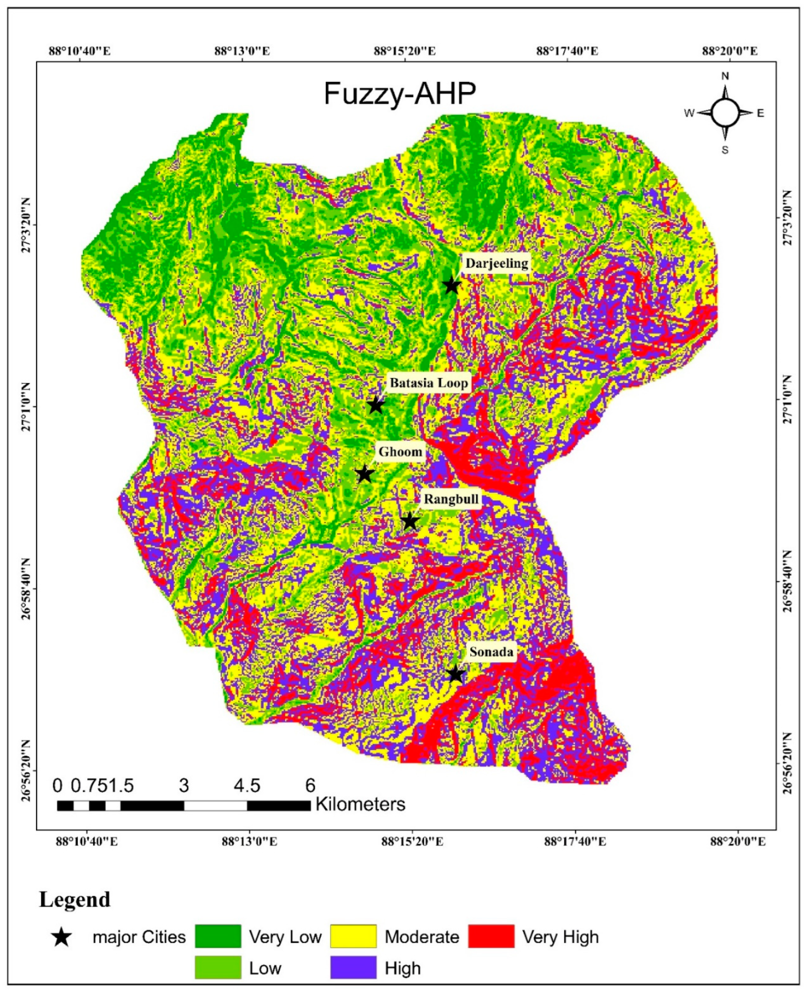
3.2.2. Assessment Using Fuzzy-AHP Model

In order to identify landslide susceptibility zones, the current study uses fuzzy set theory with AHP as a multi-criteria decision strategy. An effective and dependable method for zoning landslide susceptibility may be offered by integrating fuzzy set theory with AHP. AHP is a single procedure that assists in deciding the relative importance of numerous elements based on the advice and understanding of experts. For the current investigation, weights were allocated to the landslide determining factors (Table 5) using the AHP approach. Then, using the linear membership function, a fuzzy map of the chosen parameters for mapping landslide susceptibility was produced (MF). When creating a single layer of landslide susceptibility using the raster calculator tool of the spatial analyst in a GIS context, the weights of the parameters were determined via the fuzzy geometric mean approach (Equation (14)) (

Table 6. Fuzzy-AHP pairwise comparison matrix of landslide conditioning factors and corresponding weights, where i = lithology; ii = aspect; iii = geomorphology; iv = drainage density; v = lineament density; vi = soil type; vii = land use and land cover; viii = profile curvature; ix = rainfall; x = slope.

	i	ii	iii	iv	v	vi	vii	viii	ix	x	Weight
i	1,1,1	1/3,1/2,1/1	1/4,1/3,1/2	1/6,1/5,1/4	1/6,1/5,1/4	1/8,1/7,1/6	1/8,1/7,1/6	1/9,1/8,1/7	1/9,1/8,1/7	1/9,1/9,1/9	0.0146
ii	1,2,3	1,1,1	1/3,1/2,1/1	1/4,1/3,1/2	1/5,1/4,1/3	1/6,1/5,1/4	1/6,1/5,1/4	1/8,1/7,1/6	1/8,1/7,1/6	1/9,1/9,1/9	0.0209
iii	2,3,4	1,2,3	1,1,1	1/3,1/2,1/1	1/3,1/2,1/1	1/4,1/3,1/2	1/4,1/3,1/2	1/4,1/3,1/2	1/8,1/7,1/6	1/9,1/9,1/9	0.0327
iv	4,5,6	2,3,4	1,2,3	1,1,1	1/3,1/2,1/1	1/4,1/3,1/2	1/5,1/4,1/3	1/5,1/4,1/3	1/6,1/5,1/4	1/8,1/6,1/7	0.0427
v	4,5,6	3,4,5	1,2,3	1,2,3	1,1,1	1/3,1/2,1/1	1/4,1/3,1/2	1/6,1/5,1/4	1/7,1/6,1/5	1/8,1/6,1/7	0.0516
vi	6,7,8	4,5,6	2,3,4	2,3,4	1,2,3	1,1,1	1/3,1/2,1/1	1/4,1/3,1/2	1/4,1/3,1/2	1/6,1/5,1/4	0.0833
vii	6,7,8	4,5,6	2,3,4	3,4,5	2,3,4	1,2,3	1,1,1	1/4,1/3,1/2	1/6,1/5,1/4	1/6,1/5,1/4	0.0947
viii	7,8,9	6,7,8	4,5,6	3,4,5	4,5,6	2,3,4	2,3,4	1,1,1	1/4,1/3,1/2	1/4,1/3,1/2	0.1616
ix	7,8,9	6,7,8	6,7,8	4,5,6	5,6,7	2,3,4	3,4,5	2,3,4	1,1,1	1/4,1/3,1/2	0.2200
x	9,9,9	9,9,9	9,9,9	6,7,8	6,7,8	4,5,6	4,5,6	4,5,6	2,3,4	1,1,1	0.3344

).

$$LS{M}_{AHP}={{\displaystyle \sum }}_{i=1}^n{w}_i\ast l_i$$

(14)

where l_i is the individual factor, and w_i represents the weight for each landslide conditioning factor.

Five classes of landslide susceptibility, covering 9.39 percent, 21.86 percent, 30.86 percent, 26.27 percent, and 11.62 percent of the region, are represented in the landslide susceptibility map (Figure 7). According to the findings, 68.74 percent of the entire region falls inside the moderate to very high zone.

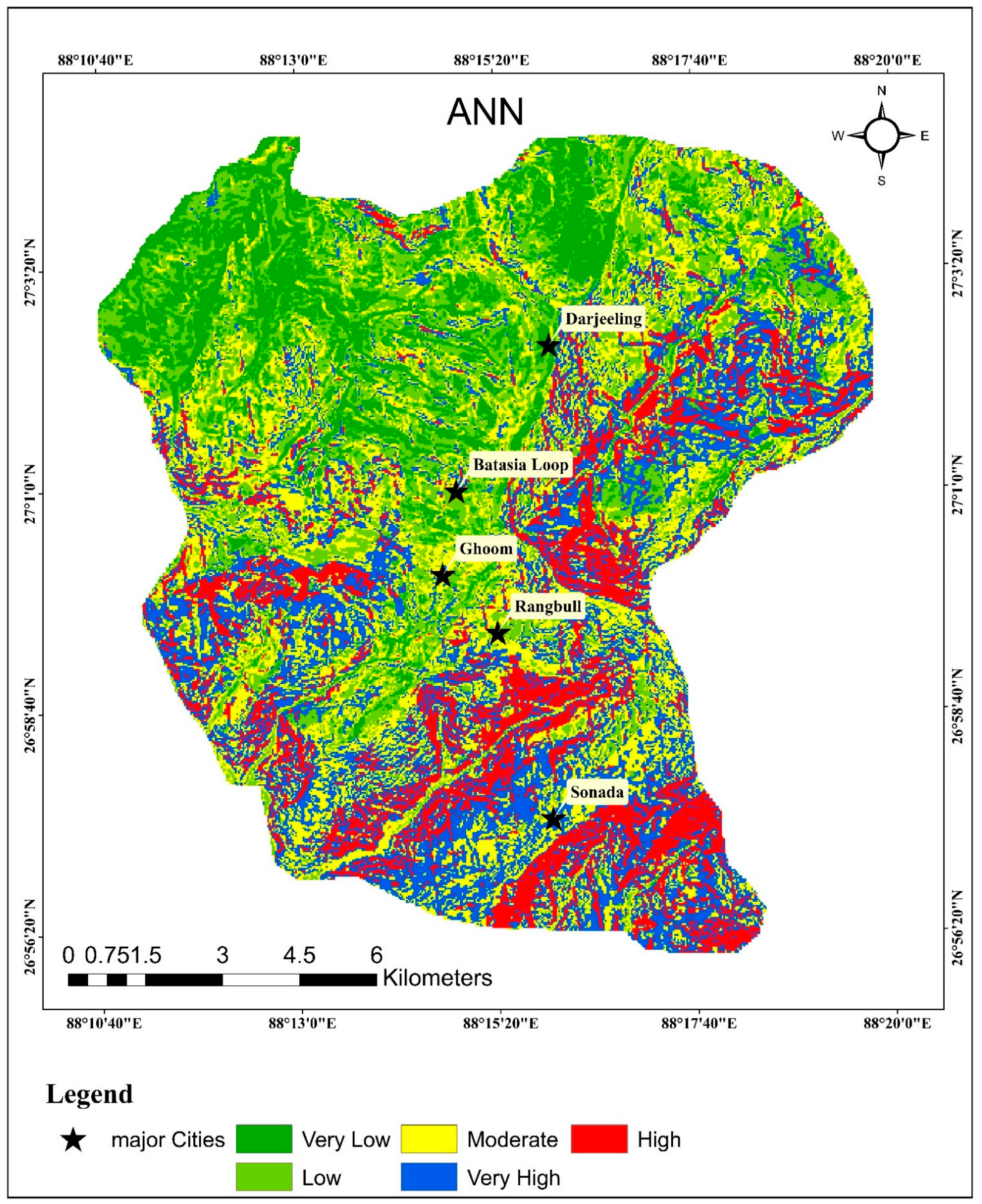
3.2.3. Assessment Using ANN Model

The MATLAB NN-toolbox was used to create a predictive evaluation model. The availability of more robust modeling and faster convergence algorithms simplifies neural net implementation. The training, target, and testing datasets were imported as matrices into the workspace. The dataset was split into two parts: 70% training data and 30% testing data. The landslide triggering factors and their parameters were included in the training samples. The corresponding landslide susceptibility class values from the study area were included in the target samples. The testing dataset was created from a subset of the study area in order to test the trained model’s performance. The appropriate model architecture was created by selecting various model parameters such as the type of network used, training function, loss parameter, number of hidden layers, and activation functions. One input layer, one hidden layer with 20 units, and one output layer comprise the ANN architecture. TRAINLM is a training algorithm for a feed-forward backpropagation neural network with a log sigmoid activation function. Figure 8a depicts the architecture of the best fit model.

The network parameters window displays the model’s training process (Figure 8b). The performance plot depicts the best performance during training by plotting the training, validation, test, and best performance curves in an epoch vs. MSE plot (Figure 8c). The sixth epoch has the best performance, with an MSE of 7.33 m. The training state with gradient and validation checks is plotted against the number of epochs (Figure 8d). A regression plot of training vs. output is also available to examine data distribution (Figure 8e). All the models were performed in Intel(R) Xeon(R) CPU E3-1245 v3 @ 3.40 GHz 3.40 GHz processor, 12 GB RAM for smooth performance.

After successfully training the model, the testing dataset was simulated. The fused output LSM layer was prepared in the GIS environment (Figure 9).

The landslide susceptibility map (Figure 9) is divided into five categories: very low, low, moderate, high, and very high landslide susceptibility zones, which cover 12.87%, 21.54%, 25.91%, 26.24%, and 13.44% area. The results show that 65.60% of the total area falls into the moderate to the very high zone.

3.3. Model Validation

The AHP, fuzzy-AHP, and ANN models’ ability to predict outcomes was evaluated using the ROC-AUC approach. The prediction curve was built using a validation dataset [66,67,68]. To validate the models in the current work, 30% of the total landslide areas (testing datasets) were employed (Figure 10). According to our findings, the performance of the neural network-based ML model ANN (AUC = 88.1%) outperforms that of the traditional statistical model AHP (AUC = 85.4%) and the fuzzy statistical method F-AHP (AUC = 86.1%). In order to give context to the evaluation values, we divided the AUC values into different groups. An acceptable model is one with an AUC between 0.75 and 0.8, a fair susceptibility model is one with an AUC between 0.8 and 0.9, and an extraordinary model is one with an AUC exceeding 0.9. Our results demonstrate that the three models we utilized had AUC values between 85% and 89%, indicating strong models for both susceptibility and functionality [13]. The outcomes of ROC analysis demonstrate that ANN performs well. In light of this, machine learning techniques based on neural networks are significantly more helpful than conventional techniques and fuzzy methods in analyzing the susceptibility of landslides.

4. Discussion

Because they are more susceptible to natural hazards, planning and development in hilly and mountainous locations must be undertaken with the utmost care. The risk of landslides is one of these. Landslides are likely to happen under the same circumstances as they did in the recent past [69]. In these places, landslide susceptibility assessments are essential because they give planners and decision-makers a first line of defense [70]. Making an accurate LSM that can be used to pinpoint regions at risk for landslides is quite challenging [71]. As a result, several strategies are being created on a regular basis all around the world to address these accuracy and dependability issues [72]. New methods have been developed as a result of the unrelenting study of LSMs. In order to create an accurate model of landslide susceptibility, our work uses MCDA, fuzzy-based MCDA, and ML-based algorithms.

Several LCF interact with triggering variables and contribute to the beginning of landslides. In order to create a precise landslide susceptibility model, it is imperative to choose suitable LCFs. As a consequence, models with high predictive ability and minimal noise are created. There are several LCFs, and they differ according to the local peculiarities. These geological, climatic, and geomorphological elements that control landslides are connected to these landslide indicators. The convex slope dominates the area’s margin, the straight slope dominates the middle portion, and the concave slope dominates the lower portion. Based on the diversity of indicators and the features of the area, there are no guidelines for choosing LCFs [73]. To choose the most suitable and stressful variables, much work has been put in. One of these initiatives is the multicollinearity test, which looks for connections between LCFs that could influence the correctness of the model as a whole. In the current study, ten LCFs were selected as independent criteria to evaluate the Hali catchment’s vulnerability to landslides. The multicollinearity of the LCFs was evaluated using the VIF. Our results demonstrate that the variables we selected do not exhibit multicollinearity. Therefore, all variables were incorporated into the models.

One of the trustworthy methods for mapping landslide susceptibility zones is the fuzzy-based AHP and ML-based approach (ANN), according to the study’s findings, which summarizes the weighted overlay analysis method utilizing MCDA (the AHP and eigenvector approaches). Ten (10) thematic layers, including slope, aspect, rainfall, lineament density, drainage density, lithology, geomorphology, soil texture, land use, and land cover, were utilized to categorize the research region into distinct landslide vulnerability zones. The landslide susceptibility map shown in Figure 6, Figure 7, and Figure 9 was produced statistically and was interpreted using the landslide susceptibility index (LSI) value. The minimum and highest LSI values for AHP were 1.63 and 7.13, respectively, with a mean value of LSI 4.35 and a standard deviation (Sd) of 0.70. (Figure 11a). The minimum and maximum values for fuzzy-AHP were 1.95 and 7.63, respectively, with a mean value of 4.99 and a Sd of 0.72. (Figure 11b). The LSI values for ANN were 3.14, 1.02, 0.17, and 6.13, respectively, for the mean, standard deviation, minimum, and maximum (Figure 11c). The landslide susceptibility index was divided into several zones according to the histogram profile. The frequency of distributed data is indicated by the histogram profile, which shows statistical information about the LSI pixel (cell) value. The natural break classification system was used for zonation mapping because the histogram demonstrated that the spread values were irregularly distributed [74]. The outcome was the identification and mapping of five classes of landslide susceptibility zones: very low susceptibility, low susceptibility, moderate susceptibility, high susceptibility, and very high susceptibility (Figure 6, Figure 7, and Figure 9). For AHP, fuzzy-AHP, and ANN, the analysis area % of the extremely high susceptibility zone is 12.31, 11.62, and 13.44, respectively (Figure 12). Fuzzy-AHP and ANN fall into the moderate to extremely high zone, respectively, according to the susceptibility area percentage of AHP, with 66.46 percent, 68.74 percent, and 65.60 percent of the region falling under this category. Therefore, we may presume that the research region as a whole is in the moderate zone.

Additionally, three susceptibility maps based on the known landslide dataset were utilized to assess the dependability of the results using the area under the curve (AUC) of the receiver operating characteristics (ROC). A map of landslide inventory was produced from published data of the Geological Survey of India. Here, 114 landslides were recorded; 79 (70 percent) were utilized as training data and 35 (30 percent) as testing data. The maps created by the ANN model appear to be more accurate than the maps created by the Fuzzy-AHP and AHP models, as shown by the AUC values of 88.1 percent, 86.1 percent, and 85.4 percent for ANN, fuzzy-AHP, and AHP, respectively. Time is a significant component in hazard studies; therefore, this discovery is helpful in an emergency. One may understand the conclusion that the models’ accuracy is equivalent. Because they can provide perfect and stable landslide susceptibility maps for risk mitigation and management planning, we advocate employing ANN, fuzzy-AHP, and AHP models in landslide investigations. A regional landslide susceptibility map may be created using the ANN model, which is also adequate and shows promise.

5. Conclusions

Landslides are one of the deadliest natural dangers in hilly terrain. The highly deformed mountainous terrain is under danger from landslides as a result of both humanmade activity and natural events (such as climate change and earthquakes) (human intervention). The northern Himalayan areas of West Bengal are becoming an unending nightmare for residents due to these dangers. To preserve lives and property, an interim and enduring solution to reducing the danger of landslides in this area is needed. We must locate and map the most susceptible places in order to assist future infrastructure and urban development plans. LSM might therefore be a crucial approach for evaluating risk management in challenging terrain. The use of MCDA models for landslide susceptibility assessments has yielded incredibly efficient and precise results for many years. In recent years, sophisticated methods known as machine learning (ML) methods have been created. This work’s main objective is to assess the effectiveness of MCDA models AHP, fuzzy-AHP, and ML methodology (ANN-) and identify the most precise and useful method for identifying landslide-prone locations in the research area. Our results (based on LSM and AUC) demonstrate the effectiveness of both conventional machine learning and deep learning techniques. The main MCDA algorithms SVM (fuzzy-AHP = 86.1 percent and AHP = 85.4 percent) were found to be inferior to the machine learning algorithm-based ANN (AUC = 88.1 percent), which performed better in terms of accuracy and predictive power. Additionally, it was shown that ANN findings were more discriminative. Overall, the landslide-prone regions and the optimal planning and development zones in the mountainous region of Darjeeling and Kurseong district, West Bengal, India, were well identified by this study. Finally, the land use planners, decision-makers, and other governmental and non-governmental organizations may use all of the LSMs created in this study as effective tools to maximize infrastructure development, resource management, and human activity in the study region.

References

1. Petley, D. Global patterns of loss of life from landslides. Geology 2012, 40, 927–930. [Google Scholar] [CrossRef]
2. Kjekstad, O.; Highland, L. Economic and social impacts of landslides. In Landslides—Disaster Risk Reduction; Springer: Berlin/Heidelberg, Germany, 2009; pp. 573–587. [Google Scholar]
3. Skilodimou, H.D.; Bathrellos, G.D.; Koskeridou, E.; Soukis, K.; Rozos, D. Physical and anthropogenic factors related to landslide activity in the Northern Peloponnese, Greece. Land 2018, 7, 85. [Google Scholar] [CrossRef] [Green Version]
4. Fan, X.; Scaringi, G.; Korup, O.; West, A.J.; van Westen, C.J.; Tanyas, H.; Hovius, N.; Hales, T.C.; Jibson, R.W.; Allstadt, K.E.; et al. Earthquake-induced chains of geologic hazards: Patterns, mechanisms, and impacts. Rev. Geophys. 2019, 57, 421–503. [Google Scholar] [CrossRef] [Green Version]
5. Dang, V.-H.; Hoang, N.-D.; Nguyen, L.-M.-D.; Bui, D.T.; Samui, P. A novel GIS-based random forest machine algorithm for the spatial prediction of shallow landslide susceptibility. Forests 2020, 11, 118. [Google Scholar] [CrossRef] [Green Version]
6. Guzzetti, F.; Mondini, A.C.; Cardinali, M.; Fiorucci, F.; Santangelo, M.; Chang, K.-T. Landslide inventory maps: New tools for an old problem. Earth-Sci. Rev. 2012, 112, 42–66. [Google Scholar] [CrossRef] [Green Version]
7. Guzzetti, F.; Carrara, A.; Cardinali, M.; Reichenbach, P. Landslide hazard evaluation: A review of current techniques and their application in a multi-scale study, Central Italy. Geomorphology 1999, 31, 181–216. [Google Scholar] [CrossRef]
8. Li, C.; Fu, Z.; Wang, Y.; Tang, H.; Yan, J.; Gong, W.; Yao, W.; Criss, R.E. Susceptibility of reservoir-induced landslides and strategies for increasing the slope stability in the Three Gorges Reservoir Area: Zigui Basin as an example. Eng. Geol. 2019, 261, 105279. [Google Scholar] [CrossRef]
9. Haque, U.; Da Silva, P.F.; Devoli, G.; Pilz, J.; Zhao, B.; Khaloua, A.; Wilopo, W.; Andersen, P.; Lu, P.; Lee, J.; et al. The human cost of global warming: Deadly landslides and their triggers (1995–2014). Sci. Total Environ. 2019, 682, 673–684. [Google Scholar] [CrossRef]
10. Froude, M.J.; Petley, D.N. Global fatal landslide occurrence from 2004 to 2016. Nat. Hazards Earth Syst. Sci. 2018, 18, 2161–2181. [Google Scholar] [CrossRef] [Green Version]
11. Dou, J.; Yunus, A.P.; Tien Bui, D.; Sahana, M.; Chen, C.-W.; Zhu, Z.; Wang, W.; Pham, B.T. Evaluating GIS-based multiple statistical models and data mining for earthquake and rainfall-induced landslide susceptibility using the LiDAR DEM. Remote Sens. 2019, 11, 638. [Google Scholar] [CrossRef]
12. Van Westen, C.J.; Castellanos, E.; Kuriakose, S.L. Spatial data for landslide susceptibility, hazard, and vulnerability assessment: An overview. Eng. Geol. 2008, 102, 112–131. [Google Scholar] [CrossRef]
13. Merghadi, A.; Yunus, A.P.; Dou, J.; Whiteley, J.; ThaiPham, B.; Bui, D.T.; Avtar, R.; Abderrahmane, B. Machine learning methods for landslide susceptibility studies: A comparative overview of algorithm performance. Earth-Sci. Rev. 2020, 207, 103225. [Google Scholar] [CrossRef]
14. Chang, K.-T.; Merghadi, A.; Yunus, A.P.; Pham, B.T.; Dou, J. Evaluating scale effects of topographic variables in landslide susceptibility models using GIS-based machine learning techniques. Sci. Rep. 2019, 9, 12296. [Google Scholar] [CrossRef] [PubMed] [Green Version]
15. Pham, B.T.; Jaafari, A.; Prakash, I.; Bui, D.T. A novel hybrid intelligent model of support vector machines and the MultiBoost ensemble for landslide susceptibility modeling. Bull. Eng. Geol. Environ. 2019, 78, 2865–2886. [Google Scholar] [CrossRef]
16. Selamat, S.N.; Majid, N.A.; Taha, M.R.; Osman, A. Landslide Susceptibility Model Using Artificial Neural Network (ANN) Approach in Langat River Basin, Selangor, Malaysia. Land 2022, 11, 833. [Google Scholar] [CrossRef]
17. Carabella, C.; Cinosi, J.; Piattelli, V.; Burrato, P.; Miccadei, E. Earthquake-induced landslides susceptibility evaluation: A case study from the Abruzzo region (Central Italy). Catena 2022, 208, 105729. [Google Scholar] [CrossRef]
18. Whiteley, J.S.; Chambers, J.E.; Uhlemann, S.; Wilkinson, P.B.; Kendall, J.M. Geophysical monitoring of moisture-induced landslides: A review. Rev. Geophys. 2019, 57, 106–145. [Google Scholar] [CrossRef] [Green Version]
19. Van Den Eeckhaut, M.; Kerle, N.; Poesen, J.; Hervás, J. Object-oriented identification of forested landslides with derivatives of single pulse LiDAR data. Geomorphology 2012, 173, 30–42. [Google Scholar] [CrossRef]
20. Ding, A.; Zhang, Q.; Zhou, X.; Dai, B. Automatic recognition of landslide based on CNN and texture change detection. In Proceedings of the 2016 31st Youth Academic Annual Conference of Chinese Association of Automation (YAC), Wuhan, China, 11–13 November 2016; pp. 444–448. [Google Scholar]
21. Yu, H.; Ma, Y.; Wang, L.; Zhai, Y.; Wang, X. A landslide intelligent detection method based on CNN and RSG\_R. In Proceedings of the 2017 IEEE International Conference on Mechatronics and Automation (ICMA), Takamatsu, Japan, 6–9 August 2017; pp. 40–44. [Google Scholar]
22. Saha, S.; Sarkar, R.; Roy, J.; Hembram, T.K.; Acharya, S.; Thapa, G.; Drukpa, D. Measuring landslide vulnerability status of Chukha, Bhutan using deep learning algorithms. Sci. Rep. 2021, 11, 16374. [Google Scholar] [CrossRef]
23. Kumar, D.; Thakur, M.; Dubey, C.S.; Shukla, D.P. Landslide susceptibility mapping & prediction using support vector machine for Mandakini River Basin, Garhwal Himalaya, India. Geomorphology 2017, 295, 115–125. [Google Scholar]
24. Roy, J.; Saha, S. Landslide susceptibility mapping using knowledge driven statistical models in Darjeeling District, West Bengal, India. Geoenvironmental Disasters 2019, 6, 1–18. [Google Scholar] [CrossRef]
25. Kanungo, D.P.; Arora, M.K.; Sarkar, S.; Gupta, R.P. A comparative study of conventional, ANN black box, fuzzy and combined neural and fuzzy weighting procedures for landslide susceptibility zonation in Darjeeling Himalayas. Eng. Geol. 2006, 85, 347–366. [Google Scholar] [CrossRef]
26. Fell, R.; Corominas, J.; Bonnard, C.; Cascini, L.; Leroi, E.; Savage, W.Z. Guidelines for landslide susceptibility, hazard and risk zoning for land-use planning. Eng. Geol. 2008, 102, 99–111. [Google Scholar] [CrossRef] [Green Version]
27. Tanyaş, H.; van Westen, C.J.; Allstadt, K.E.; Jibson, R.W. Factors controlling landslide frequency–area distributions. Earth Surf. Processes Landf. 2019, 44, 900–917. [Google Scholar] [CrossRef] [Green Version]
28. Achour, Y.; Boumezbeur, A.; Hadji, R.; Chouabbi, A.; Cavaleiro, V.; Bendaoud, E.A. Landslide susceptibility mapping using analytic hierarchy process and information value methods along a highway road section in Constantine, Algeria. Arab. J. Geosci. 2017, 10, 194. [Google Scholar] [CrossRef]
29. Mallick, J.; Singh, R.K.; AlAwadh, M.A.; Islam, S.; Khan, R.A.; Qureshi, M.N. GIS-based landslide susceptibility evaluation using fuzzy-AHP multi-criteria decision-making techniques in the Abha Watershed, Saudi Arabia. Environ. Earth Sci. 2018, 77, 276. [Google Scholar] [CrossRef]
30. Lee, S.; Sambath, T. Landslide susceptibility mapping in the Damrei Romel area, Cambodia using frequency ratio and logistic regression models. Environ. Geol. 2006, 50, 847–855. [Google Scholar] [CrossRef]
31. Greco, R.; Sorriso-Valvo, M.; Catalano, E. Logistic regression analysis in the evaluation of mass movements susceptibility: The Aspromonte case study, Calabria, Italy. Eng. Geol. 2007, 89, 47–66. [Google Scholar] [CrossRef]
32. Kanwal, S.; Atif, S.; Shafiq, M. GIS based landslide susceptibility mapping of northern areas of Pakistan, a case study of Shigar and Shyok Basins. Geomat. Nat. Hazards Risk 2017, 8, 348–366. [Google Scholar] [CrossRef] [Green Version]
33. Arabameri, A.; Pradhan, B.; Rezaei, K.; Lee, S.; Sohrabi, M. An ensemble model for landslide susceptibility mapping in a forested area. Geocarto Int. 2019, 35, 1680–1705. [Google Scholar] [CrossRef]
34. Mandal, S.; Mondal, S. Machine Learning Models and Spatial Distribution of Landslide Susceptibility. In Geoinformatics and Modelling of Landslide Susceptibility and Risk; Springer: Berlin/Heidelberg, Germany, 2019; pp. 165–175. [Google Scholar]
35. Chawla, S.; Chawla, A.; Pasupuleti, S. A Feasible Approach for Landslide Susceptibility Map Using GIS. Geotech. Spec. Publ. 2017, 2017, 101–110. [Google Scholar] [CrossRef]
36. Mandal, B.; Mandal, S. Analytical hierarchy process (AHP) based landslide susceptibility mapping of Lish river basin of eastern Darjeeling Himalaya, India. Adv. Space Res. 2018, 62, 3114–3132. [Google Scholar] [CrossRef]
37. Basu, T.; Pal, S. RS-GIS based morphometrical and geological multi-criteria approach to the landslide susceptibility mapping in Gish River Basin, West Bengal, India. Adv. Space Res. 2019, 63, 1253–1269. [Google Scholar] [CrossRef]
38. Arabameri, A.; Cerda, A.; Tiefenbacher, J.P. Spatial pattern analysis and prediction of gully erosion using novel hybrid model of entropy-weight of evidence. Water 2019, 11, 1129. [Google Scholar] [CrossRef] [Green Version]
39. Bera, A.; Mukhopadhyay, B.P.; Das, D. Landslide hazard zonation mapping using multi-criteria analysis with the help of GIS techniques: A case study from Eastern Himalayas, Namchi, South Sikkim. Nat. Hazards 2019, 96, 935–959. [Google Scholar] [CrossRef]
40. Chen, Y.; Khan, S.; Paydar, Z. To retire or expand? A fuzzy GIS-based spatial multi-criteria evaluation framework for irrigated agriculture. Irrig. Drain. 2010, 59, 174–188. [Google Scholar] [CrossRef]
41. Feizizadeh, B.; Blaschke, T. GIS-multicriteria decision analysis for landslide susceptibility mapping: Comparing three methods for the Urmia lake basin, Iran. Nat. Hazards 2013, 65, 2105–2128. [Google Scholar] [CrossRef]
42. Kolat, C.; Ulusay, R.; Suzen, M.L. Development of geotechnical microzonation model for Yenisehir (Bursa, Turkey) located at a seismically active region. Eng. Geol. 2012, 127, 36–53. [Google Scholar] [CrossRef]
43. Saaty, T.L. Decision making with the analytic hierarchy process. Int. J. Serv. Sci. 2008, 1, 83–98. [Google Scholar]
44. Zadeh, L.A. Fuzzy sets. In Fuzzy Sets, Fuzzy Logic, and Fuzzy Systems: Selected Papers by Lotfi a Zadeh; World Scientific: Singapore, 1996; pp. 394–432. [Google Scholar]
45. Balezentiene, L.; Streimikiene, D.; Balezentis, T. Fuzzy decision support methodology for sustainable energy crop selection. Renew. Sustain. Energy Rev. 2013, 17, 83–93. [Google Scholar] [CrossRef]
46. Zadeh, L.A. Studies in Fuzziness and Soft Computing: Foreword; Springer: Berlin/Heidelberg, Germany, 2010; T. 261; ISBN 9783642166280. [Google Scholar]
47. Kahraman, C.; Cebeci, U.; Ulukan, Z. Multi-criteria supplier selection using fuzzy AHP. Logist. Inf. Manag. 2003, 16, 382–394. [Google Scholar] [CrossRef]
48. Chen, V.Y.C.; Lien, H.-P.; Liu, C.-H.; Liou, J.J.H.; Tzeng, G.-H.; Yang, L.-S. Fuzzy MCDM approach for selecting the best environment-watershed plan. Appl. Soft Comput. 2011, 11, 265–275. [Google Scholar] [CrossRef]
49. Buckley, J.J. Fuzzy hierarchical analysis. Fuzzy Sets Syst. 1985, 17, 233–247. [Google Scholar] [CrossRef]
50. Can, R.; Kocaman, S.; Gokceoglu, C. A convolutional neural network architecture for auto-detection of landslide photographs to assess citizen science and volunteered geographic information data quality. ISPRS Int. J. Geo-Inf. 2019, 8, 300. [Google Scholar] [CrossRef] [Green Version]
51. Li, B.; Wang, N.; Chen, J. GIS-based landslide susceptibility mapping using information, frequency ratio, and artificial neural network methods in Qinghai Province, Northwestern China. Adv. Civ. Eng. 2021, 2021, 1–14. [Google Scholar] [CrossRef]
52. Oh, H.-J.; Lee, S. Shallow landslide susceptibility modeling using the data mining models artificial neural network and boosted tree. Appl. Sci. 2017, 7, 1000. [Google Scholar] [CrossRef] [Green Version]
53. Al-Najjar, H.A.H.; Pradhan, B. Spatial landslide susceptibility assessment using machine learning techniques assisted by additional data created with generative adversarial networks. Geosci. Front. 2021, 12, 625–637. [Google Scholar] [CrossRef]
54. Chen, W.; Chen, Y.; Tsangaratos, P.; Ilia, I.; Wang, X. Combining evolutionary algorithms and machine learning models in landslide susceptibility assessments. Remote Sens. 2020, 12, 3854. [Google Scholar] [CrossRef]
55. Arabameri, A.; Pradhan, B.; Rezaei, K. Gully erosion zonation mapping using integrated geographically weighted regression with certainty factor and random forest models in GIS. J. Environ. Manag. 2019, 232, 928–942. [Google Scholar] [CrossRef]
56. Arabameri, A.; Pourghasemi, H.R.; Yamani, M. Applying different scenarios for landslide spatial modeling using computational intelligence methods. Environ. Earth Sci. 2017, 76, 832. [Google Scholar] [CrossRef]
57. Chen, W.; Lei, X.; Chakrabortty, R.; Chandra Pal, S.; Sahana, M.; Janizadeh, S. Evaluation of different boosting ensemble machine learning models and novel deep learning and boosting framework for head-cut gully erosion susceptibility. J. Environ. Manag. 2021, 284, 112015. [Google Scholar] [CrossRef] [PubMed]
58. Zhao, P.; Masoumi, Z.; Kalantari, M.; Aflaki, M.; Mansourian, A. A GIS-Based Landslide Susceptibility Mapping and Variable Importance Analysis Using Artificial Intelligent Training-Based Methods. Remote Sens. 2022, 14, 211. [Google Scholar] [CrossRef]
59. Sengupta, A.; Nath, S.K. GIS-Based Landslide Susceptibility Mapping in Eastern Boundary Zone of Northeast India in Compliance with Indo-Burmese Subduction Tectonics. In Geospatial Technology for Environmental Hazards; Springer: Berlin/Heidelberg, Germany, 2022; pp. 19–37. [Google Scholar]
60. Tien Bui, D.; Tuan, T.A.; Klempe, H.; Pradhan, B.; Revhaug, I. Spatial prediction models for shallow landslide hazards: A comparative assessment of the efficacy of support vector machines, artificial neural networks, kernel logistic regression, and logistic model tree. Landslides 2016, 13, 361–378. [Google Scholar] [CrossRef]
61. Nhu, V.-H.; Mohammadi, A.; Shahabi, H.; Ahmad, B.B.; Al-Ansari, N.; Shirzadi, A.; Clague, J.J.; Jaafari, A.; Chen, W.; Nguyen, H. Landslide susceptibility mapping using machine learning algorithms and remote sensing data in a tropical environment. Int. J. Environ. Res. Public Health 2020, 17, 4933. [Google Scholar] [CrossRef] [PubMed]
62. Mokhtari, M.; Abedian, S. Spatial prediction of landslide susceptibility in Taleghan basin, Iran. Stoch. Environ. Res. Risk Assess. 2019, 33, 1297–1325. [Google Scholar] [CrossRef]
63. Gautam, P.; Kubota, T.; Sapkota, L.M.; Shinohara, Y. Landslide susceptibility mapping with GIS in high mountain area of Nepal: A comparison of four methods. Environ. Earth Sci. 2021, 80, 1–18. [Google Scholar] [CrossRef]
64. Sujatha, E.R.; Sridhar, V. Landslide susceptibility analysis: A logistic regression model case study in Coonoor, India. Hydrology 2021, 8, 41. [Google Scholar] [CrossRef]
65. Arabameri, A.; Pradhan, B.; Rezaei, K.; Conoscenti, C. Gully erosion susceptibility mapping using GIS-based multi-criteria decision analysis techniques. Catena 2019, 180, 282–297. [Google Scholar] [CrossRef]
66. Nam, K.; Wang, F. An extreme rainfall-induced landslide susceptibility assessment using autoencoder combined with random forest in Shimane Prefecture, Japan. Geoenvironmental Disasters 2020, 7, 6. [Google Scholar] [CrossRef] [Green Version]
67. Azarafza, M.; Azarafza, M.; Akgün, H.; Atkinson, P.M.; Derakhshani, R. Deep learning-based landslide susceptibility mapping. Sci. Rep. 2021, 11, 24112. [Google Scholar] [CrossRef]
68. Xing, Y.; Yue, J.; Guo, Z.; Chen, Y.; Hu, J.; Travé, A. Large-scale landslide susceptibility mapping using an integrated machine learning model: A case study in the Lvliang Mountains of China. Front. Earth Sci. 2021, 622. [Google Scholar] [CrossRef]
69. van Westen, C.J.; van Asch, T.W.J.; Soeters, R. Landslide hazard and risk zonation-Why is it still so difficult? Bull. Eng. Geol. Environ. 2006, 65, 167–184. [Google Scholar] [CrossRef]
70. Roccati, A.; Paliaga, G.; Luino, F.; Faccini, F.; Turconi, L. GIS-based landslide susceptibility mapping for land use planning and risk assessment. Land 2021, 10, 162. [Google Scholar] [CrossRef]
71. Mandal, K.; Saha, S.; Mandal, S. Applying deep learning and benchmark machine learning algorithms for landslide susceptibility modelling in Rorachu river basin of Sikkim Himalaya, India. Geosci. Front. 2021, 12, 101203. [Google Scholar] [CrossRef]
72. Prakash, N.; Manconi, A.; Loew, S. A new strategy to map landslides with a generalized convolutional neural network. Sci. Rep. 2021, 11, 9722. [Google Scholar] [CrossRef]
73. Park, S.; Kim, J. Landslide susceptibility mapping based on random forest and boosted regression tree models, and a comparison of their performance. Appl. Sci. 2019, 9, 942. [Google Scholar] [CrossRef] [Green Version]
74. Constantin, M.; Bednarik, M.; Jurchescu, M.C.; Vlaicu, M. Landslide susceptibility assessment using the bivariate statistical analysis and the index of entropy in the Sibiciu Basin (Romania). Environ. Earth Sci. 2011, 63, 397–406. [Google Scholar] [CrossRef]
Figure 1. Location of the study area.
Land 11 01711 g001
Figure 2. Graphical representation of overall methodology.
Land 11 01711 g002
Figure 3. Landslide conditioning factors including landslide inventory: (a) landslide inventory; (b) slope; (c) aspect; (d) profile curvature; (e) drainage density; (f) soil texture; (g) geomorphology; (h) lithology; (i) lineament density; (j) rainfall; (k) LULC.
Land 11 01711 g003aLand 11 01711 g003bLand 11 01711 g003c
Figure 4. Triangular fuzzy member (TFM) M ˜ .
Land 11 01711 g004
Figure 5. The basic structure of ANN.
Land 11 01711 g005
Figure 6. Landslide susceptibility map using AHP.
Land 11 01711 g006
Figure 7. Landslide susceptibility map using fuzzy-AHP.
Land 11 01711 g007
Figure 8. ANN model for LSM: (a) mole architecture; (b) model’s define parameters; (c) model performance (training); (d) model training state; (e) regression plot (training, test, validation, and overall).
Land 11 01711 g008aLand 11 01711 g008b
Figure 9. Landslide susceptibility map using ANN model.
Land 11 01711 g009
Figure 10. Overall accuracy curves for AHP, fuzzy-AHP, and ANN models.
Land 11 01711 g010
Figure 11. Histogram analysis of LSM model: (a) AHP; (b) fuzzy-AHP; (c) ANN.
Land 11 01711 g011
Figure 12. Graph showing distribution of area percentage of different classes.
Land 11 01711 g012