1. Introduction
Economic spatial structure has always been a hot research topic. The classic location theory of von Thünen and Weber, the growth pole theory, the trickle-down theory, the spatial interaction theory, and the “core–periphery” theory proposed by the middle of the 20th century all explore the spatial structure from the perspective of inter-regional interaction [
1,
2,
3]. With the continuous development of science and technology, people’s understanding of the existing space and distance has been continuously developed and improved. Time distance and cost distance have gradually replaced traditional space distance [
4]. The development of transportation technology will shorten the travel time between cities, lead to changes in the relative location structure between cities [
5,
6,
7,
8], and then have an impact on the economic spatial restructuring [
9,
10,
11]. As a major innovation in the history of railway transportation, the rapid development of high-speed railway (HSR) is bound to affect human spatial behavior patterns, change the pattern of traditional economic relations between regions, and reshape the regional economic spatial pattern, which makes it the most important mode of travel between regions [
12,
13,
14]. As such, the railway transport network structure composed of the conventional railway (CR) and HSR can provide a new and important way to understand the economic spatial structure of a country.
China is a populous country with a vast territory, and railway is the main mode of intercity travel. The construction of China’s railway system initially lagged behind those of developed western countries. At the founding of the People’s Republic of China in 1949, the operating mileage of the country’s railway was only 21,800 km, and by the 1990s the average speed of China’s trains was less than 60 km/h [
15]. The railway system subsequently underwent six major stages of increases in the speed of trains. On 1 August 2008, as the Beijing Olympics were about to be held, the Beijing–Tianjin intercity railway, with a design speed of 350 km/h, began operation. This marked China’s entry into the era of HSR. Since then, the construction of HSR has progressed impressively, and CR network and HSR network coexist and operate simultaneously. In 2019, China’s railway passenger turnover was 1470.66 billion person-km [
16].
In this paper, we analyzed the characteristics of China’s railway transport network, and based on this, we further identified the economic spatial structure through a new computational algorithm. It advances the existing literature on railway networks in at least three aspects: (i) analyzing the national railway transport structure to explore China’s economic spatial transformation; (ii) identifying the urban hierarchy and economic regionalization using the proposed hierarchical analysis algorithm based on the railway transport network; (iii) based on the identified economic regionalization, exploring the city rank-size distribution and the law of the primate city in a developing country with large territory. The rest of the paper is structured as follows:
Section 2 summarizes the literature concerning the HSR and economic spatial structure;
Section 3 presents the data and the methods used; in
Section 4, we discuss the characteristics of China’s railway transport network;
Section 5 analyzes the economic spatial structure based on railway transport network;
Section 6 and
Section 7 conclude and discuss this study.
2. Literature Review
In 1986, Friedmann pointed out the importance of urban hierarchical network structure research from the perspective of urban agglomerations in the world city theory. He believed that cities are arranged “into a hierarchy of spatial connections, roughly in line with their economic strength” [
14]. Krugman, Scott, and Masahisa then introduced econometric methods to study economic spatial structure. In recent years a great deal of research methods for the economic spatial structure have emerged, such as coefficient of variation, Theil index, ellipse standard deviation, and kernel density analysis [
17,
18,
19], GWR model [
20], system dynamics (SD), cellular automata (CA), pressure–state–response model (PSR), expansion index model (AGI), and other methods [
21]. These studies tried to sum up the characteristics, connotations, and evolution of the economic spatial structure by calculating the indices for each city [
22,
23,
24]. The frequently used data are fixed economic indicators, such as per capita GDP, fixed asset investment, and residents’ income. However, the economic spatial structure includes not only the development level of each city but also the connections between them. To date, few studies have combined data of traditional statics regarding urban development level with data of dynamic transportation connections. Studying the economic spatial structure through the combination of these kinds of data can lead to results that are much closer to reality, which is of academic significance.
With the rapid development and rising role of railway transport, there has been a considerable amount of research into railway transport. These studies fall into three classifications: (i) those focusing on the structure of the railway transport network [
25,
26]; this type of research aims to analyze how the characteristics of the railway network change during its upgrade, and the frequently used indices includes the alpha index, gamma index, beta index, and the diameter of the network; (ii) studies focusing on how railway upgrading impacts the accessibility or connectivity of cities or regions; HSR can improve accessibility to the areas along the line, but its degree of influence varies with the location, scale, and basis of development of a given region or city [
27,
28,
29]; (iii) the third line of research focuses on how HSR impacts regional economic development [
30,
31]; however, there is still no consensus. Among those studies, some hold that HSR promotes an increase in population, employment, gross domestic product (GDP) and local budgets [
32,
33,
34] and has a positive effect on the coordinated development of the regional economy [
35,
36,
37], but some hold the opposite or neutral view [
38,
39,
40]. The impact of HSR on the economic disparity is also controversial.
Although there have been some studies on the spatial effects of railway transport, there is still little attention paid to the economic spatial structure which underlines and is reflected by railway network structure. The existing literature shows the consensus that transport is closely related to regional economic development, and more-developed regions normally have more train services. However, little attention has been paid to the overall economic regionalization all over the country as reflected by the deployment of train services, i.e., the railway transport structure, and even less attention has been paid to the difference between the sub-networks of traditional CR and HSR, which has considerable implications for regional economic spatial transformation.
3. Data and Methods
3.1. Data
The data for this study were collected in three parts. (1) The national railway passenger train schedules in April 2017, including those for railway lines and stations, were obtained [
41], covering 5483 trains, 2826 stations, and 5,435,594 km of railway tracks. A city with multiple stations is considered one node in the city network. (2) The 1:4 million Database of the National Fundamental Geographic Information System of China was obtained from the Thematic Database for the Human–Earth System of the Chinese Academy of Sciences. (3) Socioeconomic data were obtained from the provincial statistical yearbooks of 2018, the China City Statistical Yearbook 2018, and the prefecture Statistical Communiqué of National Economic and Social Development 2017.
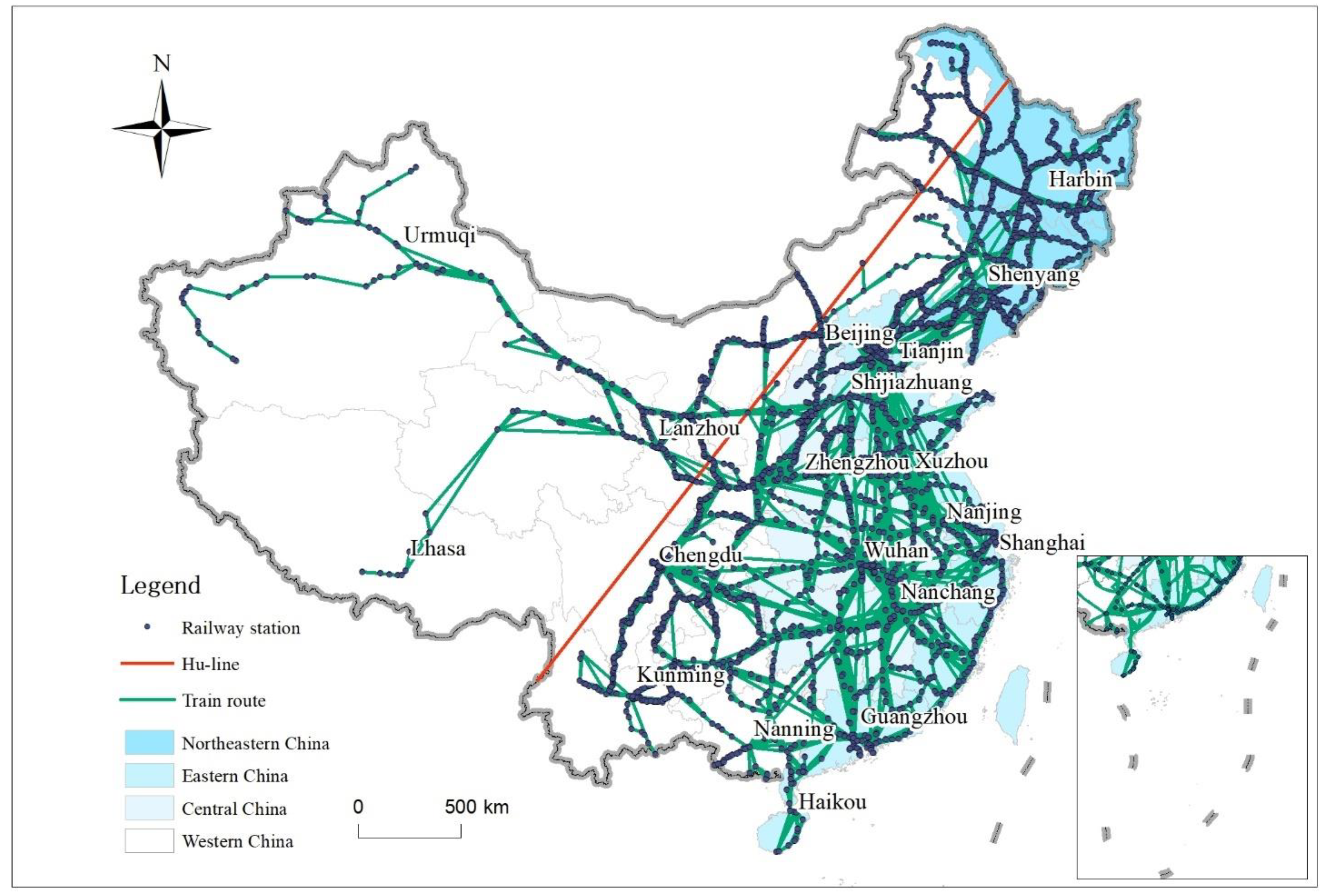
China has 337 prefecture-level cities and municipalities, and we examined 318 of these where train stations were located (some county-level cities were merged). The spatial distributions of China’s railway stations and train tracks are shown in
Figure 1. There are 2433 and 393 train stations on the east and west sides of the Hu line, respectively, accounting for 86% and 14% of the total number of stations, respectively. Of these there are 498 and 22 HSR stations, respectively, accounting for 96% and 4% of the total, respectively.
Table 1 gives the distribution of stations in four major regions of China. The number of train stations in the east, middle, west, and northeast accounted for 20.6%, 17.6%, 37.5%, and 24.3%, respectively, of the total number of stations, and the number of HSR stations accounted for 42.7%, 29.4%, 21.4%, and 6.5%, respectively. The ratio of HSR stations in the eastern region was much higher than that of traditional train stations, which indicates that the upgrading of trains in China is focused on the eastern coastal areas.
3.2. Nodal Centrality Measures
We denote by the graph G = (V, E) the railway transport network of China, where V = {vi, i = 1, 2, …, n} is the set of cities with stations and E = {ei, i = 1, 2, …, n} is the set of track sections between two adjacent cities. If a train is operating between cities with one or more intermediate stations, then these cities are considered adjacent to each other and there is an edge between them. The network can be characterized as an unweighted n × n matrix A with elements aij; if cities i and j are adjacent, then aij = 1, otherwise aij = 0.
There is a wealth of literature on evaluating network connectivity [
6,
43,
44,
45]. Borgattie reviewed network analysis in the social sciences and summarized its difference between social and physical sciences [
46]. The paper begins with indices due to Freeman [
47,
48], i.e., degree centrality (
DC), closeness centrality (
CC), and betweenness centrality (BC), which are widely used to measure the connectivity among network nodes. These centralities provide the basis for further analysis.
(1) The
DC of a node is the number of edges that it shares with other nodes, and it symbolizes the importance of that node to the network. The
DC of node
i reflects its accessibility in the network and is defined as
where
aij = 1 when there is an edge between nodes
i and
j, otherwise
aij = 0.
(2) The
CC of a node is the inverse of the average shortest distance between it and each of the other nodes in a given network [
49]. The
CC measures the extent to which a node is close to all other nodes, and it reflects its accessibility in a given network. The shorter the distance between the node and neighboring nodes, the higher its
CC, and the more convenient it is to reach the other nodes. The
CC of node
i is written as
where
is the length of the edge connecting nodes
i and
j.
(3) The
BC of a node measures the extent to which it lies between other nodes in a network [
50]. A node tends to be more powerful if it is along the shortest paths connecting many node pairs because it may then be in a position to broker or mediate connections between these pairs. The betweenness of a node is defined as the ratio of all shortest paths passing through it, and reflects its transitivity. The
BC of node
i is written as
where
quantifies the number of times that node
i is an intermediary node along the shortest path between nodes
j and
k, and
denotes the sum of all shortest paths between nodes
j and
k.
3.3. Computer Algorithm for Establishing Urban Hierarchy
According to central place theory, regional spatial interactions have a hierarchical structure, i.e., larger cities have larger radiation area which covers those of smaller cities, thus forming a hierarchical regional spatial structure. Therefore a tree structure is used to characterize the urban hierarchy, and a hierarchical analysis algorithm was developed to identify the urban hierarchy based on city attractiveness and the strength of intercity connections. The DC characterizes the attractiveness of a node city. A city with higher attractiveness usually has larger population, so city population was combined with DC to evaluate city attractiveness more reasonably. City attractiveness is the weighted sum of DC and population.
The logic of the algorithm is that if city A is in the hinterland of city B, then city B has higher attractiveness than city A, and among all the cities that have higher attractiveness than city A, city B has the highest connection with city A. City B is set as the father node of city A in the urban hierarchy. The algorithm circulates to find the father nodes of all the cities (except for the root) to build the hierarchy, i.e., a tree. A flowchart of the algorithm is shown in
Figure 2.
4. Characteristics of China’s Railway Transport Network
4.1. Centralities of Node Cities in Overall Railway Transport Network
4.1.1. Spatial Pattern of Centralities of Node Cities
The patterns of spatial distribution of the three centrality indicators are shown in
Figure 3. Cities located in the east and center were more connected than those in the west. Moreover, cities with high DC and CC were mostly located along the trunk HSR lines in the eastern and central regions, this being defined as the “corridor effect” (see
Figure 3). Cities with higher DC were concentrated along the Beijing–Shanghai line, the Beijing–Guangzhou line in the north–south direction, and the Shanghai–Kunming, Shanghai–Chengdu, and Shanghai–Xuzhou–Xi’an–Urumqi lines in the east–west direction. The spatial distribution of BC was different. Cities with high BC were mainly provincial capitals or those located along the Beijing–Shanghai line, indicating that train transfer mainly occurred at provincial capitals and municipalities to form a hub-and-spoke structure, with provincial capitals and municipalities as the main nodes.
4.1.2. Statistical Characteristics of Centralities of Node Cities
The city centrality values of the indicators of degree, closeness, and betweenness were fitted to the model
(
Table 2), where
y is the centrality,
x is the rank of the centrality indicators, and
q is the empirical coefficient (slope) that partially captures the rules of distribution of city centrality. The higher the value of
q, the fewer cities there are at the highest level of the network in terms of city centrality. Each centrality decreased exponentially, and the DC distribution of cities decreased the most slowly (
q was −0.0011), indicating that changes in the accessibility of each city were relatively gentle. Moreover, the fitted curve for BC was the steepest (
q was −0.023), and that for CC was in the middle (
q was −0.002). The drastic change in BC indicates that a few hub cities undertake most of the transfer function.
4.1.3. Accessibilities of Megacities
Three megacities, i.e., Beijing, Shanghai, and Guangzhou, are leading China’s economic development.
Table 3 lists the number of cities that could be reached directly from these megacities, the number of departing trains, and the number of departing high-speed trains in these three megacities. The number of cities that could be reached directly from Beijing was higher than those that could be reached from Shanghai and Guangzhou, accounting for 37% of the total. In terms of the number of departing trains, Beijing was slightly above Shanghai, and Guangzhou had the fewest of the three. However, the number of HSRs originating from Shanghai exceeded that from Beijing. Widespread HSR construction is relatively recent, so the deployment of trains in service in the renewal process indicates the shift in China’s economic center of gravity to the southeast (further analysis is provided below).
4.2. Intercity Connectivity Based on Overall Railway Transport Network
Figure 4 shows the intercity connection network, where the width of the lines denotes the intercity relational strength, which was divided into four levels using the natural breakpoint method. The first level of connections was mainly among Beijing, Shanghai, Guangzhou, Nanjing, and other metropolises, which formed the backbone of the railway transport network, with Shanghai and Beijing at its heart, while such sub-centers as Zhengzhou, Chongqing, and Xi’an formed the second level, with such important lines as the Zhengzhou–Xi’an–Lanzhou and Chengdu–Chongqing ones in western China. Other provincial capitals were connected by the third level of network. The top tier of the railway transport network was distributed to the east of the Hu line. At the second level, only cities—Lanzhou, Turpan, and Urumqi—were located to the west of the Hu line. This shows that although the network had expanded, most of the demand had increased east of the line. Among the 5483 trains in service, 4625 ran only east of the Hu line (84.4%), 241 trains ran only to its west (4.4%), and 617 trains ran across the Hu line (11.3%), which shows that the interactions among western cities and between western and eastern cities were very weak.
To further analyze the connection between specific cities, a directed intercity network was established to calculate the shortest distance between each city pair (the number of edges along the shortest path).
Figure 5a shows the shortest distance between pairs of the top 20 cities in terms of DC (normally developed cities). Most such cities were connected by direct trains. Transfers were required for only a few city pairs, which indicates that it is very convenient to travel between these cities.
Figure 5a also shows a certain symmetry, indicating that the incoming and outgoing rail journeys between cities were fairly even.
Figure 5b shows the shortest distances between pairs of the bottom 20 cities in terms of DC (normally developing cities). It is clear that commuters between cities in this group usually needed to transfer more than twice to reach their destinations. In addition, compared with developed cities, symmetric transport was absent between developing cities.
Further analysis of the connections between developed and developing cities shows that the average distance between the bottom and top 20 cities in terms of DC was 2.2, i.e., most of the bottom 20 cities could make it to the top 20 cities with one transfer. This indicates that the transport between developing and developed cities was more convenient than that between developing cities. This phenomenon shows that the developing cities were mainly connected to developed cities and formed their hinterland, but the connection between developing cities was weak and lacked a systematic and symmetrical transport development plan.
4.3. Distribution Characteristics of Train Service in Terms of Population
In
Figure 6, the size of a node denotes the total number of stopover trains of the corresponding city. As can be seen, the most trains were in service in Beijing, followed by Shanghai, Nanjing, Wuhan, Guangzhou, and Wuxi, all of which are cities in the eastern region except for Wuhan. However, this was not the case for the distribution of the train service intensity, which shows the number of trains in service in the context of the local population. The train service intensity of city
i, i.e.,
, is calculated as
where
Pi and
Ti are the population and number of all the trains in service in city
i, respectively, and
TtlPop and
TtlTrain are the total national population and total number of national trains in service, respectively.
The cities shown in
Figure 6 are classified into three groups: (i) cities with a train service proportion greater than the population proportion, (ii) those with a train service proportion less than the population proportion, and (iii) those with no train service. Some of the cities with a high train service intensity were developed cities (such as Beijing, Shanghai, and Guangzhou) and transport hubs (e.g., Wuhan, Zhengzhou, and Xi’an); the others were those along the railway lines that connect developed cities, e.g., the Beijing–Shanghai and Shanghai–Urumqi lines. Cities without train services were mainly located on the Tibet Plateau, which is mountainous and scarcely populated. From
Figure 4, most of the trains in service were concentrated in the central and eastern regions, but considering population distribution, China’s train services were evenly distributed across regions.
5. Economic Spatial Structure Based on Railway Transport Network
5.1. Migration of China’s Economic Center of Gravity
China is now upgrading its railway transport by constructing HSR, so CR and HSR coexist currently. The railway department in China has been unclear about the basis for its deployment of trains, but the most likely scenario is that it would consider the local population and economic development [
15]. Therefore, any change in city accessibility or connectivity while upgrading the train service from CR to HSR implies economic spatial transformation.
Table 4 gives the rankings of provincial capitals and cities at or above sub-provincial administrative level (excluding cities without HSR stations) in terms of DC in different sub-networks, i.e., CR and HSR. Beijing was ranked the highest in terms of DC in both CR and HSR, which indicates that Beijing had the highest connectivity all the time during railway upgrading. The rankings of cities in northeast China dropped significantly from CR to HSR (yellow signs). Shenyang, the capital of the Liaoning Province in northeast China, ranked fifth in terms of CR connectivity, while its ranking dropped significantly in terms of HSR connectivity. Two other provincial capitals in the region, i.e., Harbin and Changchun, exhibited similar situations. The degrees of change in some western cities are marked with green in
Table 4. The rankings of these cities in terms of HSR were on a downward trend compared with CR. Cities with a significant increase in rankings were mainly located in southern China or coastal areas, e.g., Nanjing, Ningbo, and Shenzhen.
We conclude here that the importance of cities in northern and western China exhibited a downward trend from CR to HSR, which indicates that China’s economic center of gravity is shifting to coastal areas while also moving south. This change is not obvious in the overall railway transport network.
5.2. Economic Regionalization in China
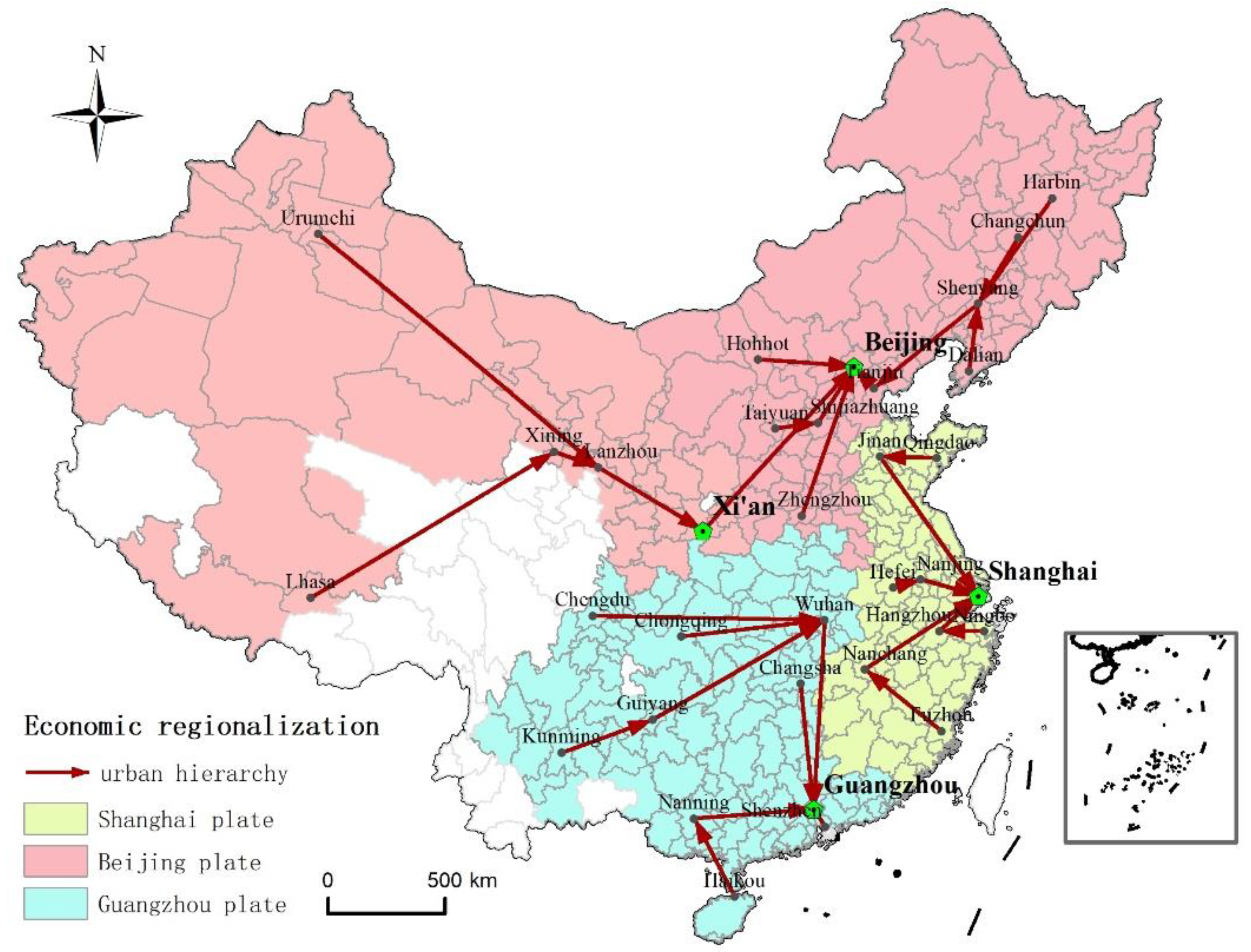
The following assumptions were made in the present study: (i) the more train service between a city pair, the more connection between them; (ii) the higher the attractiveness of a city, the higher its level in the urban hierarchy. The developed algorithm (see
Section 3.3 for details) was then used to generate the urban hierarchy based on the overall railway transport network. For clarity, only the hierarchy of cities of provincial capitals and cities at or above sub-provincial administrative level is shown in
Figure 7; see the
Appendix A for the detailed hierarchy.
Provincial capitals and cities at or above sub-provincial administrative level are normally economically developed cities. Each of them had its own hinterland (son nodes), which adjoined each other to form the service areas of the root megacities, i.e., Beijing, Shanghai, and Guangzhou. Each megacity together with its service areas forms the new economic geography of three economic plates (
Figure 7). Beijing’s service area was mainly from north China and northeast China where the economy is now relatively backward, that of Shanghai was mainly in east China, and that of Guangzhou was mainly in south and southwest China.
Next, the city rank-size distribution by economic plate was calculated. The rank-size distribution and city primacy index are two important means of measuring urban systems. The rank-size distribution describes the relationship between the size of a city and its ranking. In 1936, Singer proposed the rank-size distribution based on Auerbach and Lotka’s research [
51,
52], i.e.,
Pi =
P1/(
Riq), where
Pi is the population of city
I in the country,
P1 is the population of the largest city,
Ri is the rank of city
i in terms of population, and
q is an empirical coefficient; the higher the value of
q, the greater the difference in the size of urban population, whereas the lower the value of
q, the more balanced the sizes of the cities. The case of
q = 1 corresponds to Zipf’s law [
53,
54]. We take the logarithm of both sides to obtain
However, previous studies have shown that the rank-size distribution of cities in China is difficult to explain [
55], given that it does not correspond to any known rule of rank-size distribution. China is a vast country with great differences in development and marketization, thus forming different economic plates, so we hypothesize that in each economic plate, cities should be more in line with the rule of rank-size distribution represented by Equation (5). Accordingly, we further analyzed the city rank-size distribution by economic plate as identified in
Section 4.1. Using the permanent resident population of each city in 2017 as the city size, we performed a regression analysis of the rankings of each economic plate, and the results are given in
Table 5.
The adjusted R2 by economic plate was significantly higher than that at the national level, which means that the law of rank-size distribution became more significant in each economic plate. This confirmed the previous hypothesis, i.e., cities in each economic plate are more in line with the rule of rank-size distribution represented by Equation (5). This in turn confirmed that the economic spatial structure identified above is reasonable, and new economic plates have formed in China.
The Beijing plate had the highest values of the coefficient q, followed by the Shanghai and Guangzhou plates. This indicates that the Beijing plate had the largest regional disparity. In terms of overall economic development, the Beijing plate was lower than the Shanghai and Guangzhou plates, so we conclude that regions that are more economically developed become more balanced internally.
The primacy indices (The city primacy index is the ratio of the population size of a country’s largest city to that of its second-largest city; if this value is 2, then the largest city is twice the size of the second-largest city. The city primary index of a country is usually closer to 2, which is called the law of the primate city.) of the Beijing, Shanghai, and Guangzhou plates were calculated to be 1.4, 2.2, and 1.9, respectively. Thus, the two more-developed regions, i.e., the Shanghai and Guangzhou plates, were more in accord with the law of the primate city. Combined with the fact that the city primacy index was proposed in the context of small research areas [
56,
57], mostly featuring developed countries, it can be concluded that in a developing country with a vast territory such as China, the law of the primate city is not prominent in the entire region.
6. Conclusions
This study systematically explored China’s railway structure by different networks, i.e., the CR and HSR networks and the overall network, and examined the national economic spatial structure and its evolution process at the prefecture city levels (including municipalities) based on the railway structure. The main findings of this study are as follows.
First, a few hub cities undertook most of the transfer function in China; backward cities not only had fewer train services but lacked symmetrical traffic plans, and they had stronger connections with developed cities than among themselves, thereby forming a hub-and-spoke structure; From the changes in rankings of cities by train type, we conclude that the importance of cities in northern and western China exhibited a downward trend from CR to HSR, which indicates that China’s economic center of gravity is shifting to coastal areas while also moving south.
Second, the national urban hierarchy was established through the proposed hierarchical analysis algorithm, and based on the urban hierarchy study identified the economic spatial structure of three plates based, i.e., economic plates of Beijing, Shanghai, and Guangzhou. The Beijing plate was mainly from north China and northeast China where the economy is now relatively backward; that of Shanghai was mainly in east China, and that of Guangzhou was mainly in south and southwest China.
Third, the law of rank-size distribution became more significant in each economic plate. This showed that the law of the primate city is not prominent in a developing country with a large territory such as China.
7. Discussion
The HSR construction brings new vitality and new opportunities to regional economic development. This study shows that China’s economic center of gravity is moving to the southeast coast, and the links between backward cities have not been significantly strengthened. There is no balance between fairness and efficiency. Therefore, in the future, underdeveloped areas in the northwest of China should accelerate their integration into the national rapid transit network. Against to the background of China’s “One Belt, One Road” and Western Development Strategy, to moderately promote the construction of HSR in underdeveloped areas is important for realizing the cooperation between China’s hinterland and coastal area.
This paper identified the economic spatial structure of three plates, which helped reveal the macroeconomic regionalization of China and provide valuable reference for further research into China’s economic spatial transformation. The economic spatial structure identified also provides a scientific basis for regional economic restructuring and regional coordinated development decision-making. However, we do not claim that regionalization identified is an accurate economic zoning. First, a few regions with no train service were excluded. Second, the identified economic plates cross provincial administrative boundaries, thereby causing considerable management difficulties. Third, more factors—e.g., economic connection, road transport, airlines—should be considered to identify economic zones. Nevertheless, the results are somewhat reasonable given that economic spatial pattern is an important consideration of transport deployment.
This paper finds that the law of the primate city is more significant in each economic plate than in the whole country. It provides a reasonable explanation for the divergent opinions on the characteristics of the city rank-size distribution in China. However, further empirical research is needed to prove this conclusion based on more countries or regions as cases.
A few aspects of this study remain to be improved. First, examination of regional characteristics in this study was limited to the train network. Other factors such as aviation and road transport, population migration, and intercity trade also shape the economic spatial structure, so these factors should also be considered in future work to improve the research. Second, this research concluded that China’s economic center of gravity is shifting southeast but did not reveal the underlying mechanism. Third, the fact that city rank-size distribution by economic plate is more in line with the law of the primate city raises another question worth considering, i.e., how many megacities are most suitable in China and how to distribute them?
Author Contributions
This study was conducted under cooperation between F.N. and F.W. Conceptualization, F.N. and F.W.; methodology, F.N.; software, F.N.; validation, F.W.; formal analysis, F.N.; investigation, F.W.; data curation, F.W.; writing—original draft preparation, F.N.; writing—review and editing, F.W.; visualization, F.W.; supervision, F.W.; funding acquisition, F.N. and F.W. All authors have read and agreed to the published version of the manuscript.
Funding
This research was funded by the Strategic Priority Research Program of Chinese Academy of Sciences, grant number XDA19040401; the National Natural Science Foundation of China, grant number 42071153 and 41801149; Young Talents of Science and Technology in Universities of Inner Mongolia, grant number NJTY-20-B09.
Data Availability Statement
Publicly available datasets were analyzed in this study. A part of the data can be found here: [
https://www.12306.cn/index/], accessed in April 2017.
Conflicts of Interest
The authors declare no conflict of interest.
Appendix A
Figure A1.
Urban Hierarchy.
Figure A1.
Urban Hierarchy.
References
- Von Thünen, J.H. Der Isolierte Staat in Beziehung auf Landwirtschaft und Nationalökonomie, 2nd ed.; Jena, G., Ed.; Fischer: Stuttgart, Germany, 1910. [Google Scholar]
- Webber, A. Umber den Standort der Industruction. Theory of the Location of Industries; University of Chicago Press: Chicago, IL, USA, 1909. [Google Scholar]
- Friedman, J.R. Regional Development Policy—A Case Study of Venezuela; The MIT Press: Cambridge, MA, USA, 1966. [Google Scholar]
- Banister, D.; Berechman, J. Transport Investment and Economic Development; Routledge: London, UK, 2000. [Google Scholar]
- Albalate, D.; Bel, G. High-speed rail: Lessons for policy makers from experiences abroad. Public Adm. Rev. 2012, 72, 336–349. [Google Scholar] [CrossRef]
- Sasaki, K.; Ohashi, T.; Ando, A. High-speed rail transit impact on regional systems: Does the Shinkansen contribute to dispersion? Ann. Reg. Sci. 1997, 31, 77–98. [Google Scholar] [CrossRef]
- Jiao, J.; Wang, J.; Zhang, F.; Jin, F.; Liu, W. Roles of accessibility, connectivity and spatial interdependence in realizing the economic impact of high-speed rail: Evidence from China. Transp. Policy 2020, 91, 1–15. [Google Scholar] [CrossRef]
- Liang, Y.; Zhou, K.; Li, X.; Zhou, Z.; Sun, W.; Zeng, J. Effectiveness of high-speed railway on regional economic growth for less developed areas. J. Transp. Geogr. 2020, 82, 102621. [Google Scholar] [CrossRef]
- Kansky, K.J. Structure of Transportation Networks: Relations between Network Geometry and Regional Characteristics; University of Chicago: Chicago, IL, USA, 1963. [Google Scholar]
- Vickerman, R. Can high-speed rail have a transformative effect on the economy? Transp. Policy 2018, 62, 31–37. [Google Scholar]
- Zhou, Y.; Kundu, T.; Goh, M.; Sheu, J.B. Multimodal transportation network centrality analysis for Belt and Road Initiative. Transp. Res. Part E Logist. Transp. Rev. 2021, 149, 102292. [Google Scholar] [CrossRef]
- Debrezion, G.; Pels, E.; Rietveld, P. Modelling the joint access mode and railway station choice. Transp. Res. Part E Logist. Transp. Rev. 2009, 45, 270–283. [Google Scholar] [CrossRef]
- Wu, K.; Fang, C.; Zhao, M.; Chen, C. The intercity space of flow influenced by high-speed A case study for the rail transit passenger behavior between Beijing and Tianjin. Acta Geogr. Sin. 2013, 68, 159–174. (In Chinese) [Google Scholar]
- Román, C.; Martín, J.C. Integration of HSR and air transport: Understanding passengers’ preferences. Transp. Res. Part E Logist. Transp. Rev. 2014, 71, 129–141. [Google Scholar] [CrossRef]
- Zheng, S.Q.; Kahn, M.E. China’s bullet trains mitigate the cost of mega city growth. Proc. Natl. Acad. Sci. USA 2013, 110, E1248–E1253. [Google Scholar] [CrossRef]
- National Bureau of Statistics. Statistical Bulletin of the People’s Republic of China on the 2019 National Economic and Social Development. 2020. Available online: http://www.stats.gov.cn/tjsj/zxfb/202002/t20200228_1728913.html (accessed on 1 September 2019).
- Proost, S.; Thisse, J.F. What can be learned from spatial economics? J. Econ. Lit. 2019, 57, 575–643. [Google Scholar] [CrossRef]
- Dingel, J.I.; Miscio, A.; Davis, D.R. Cities, lights, and skills in developing economies. J. Urban Econ. 2021, 125, 103174. [Google Scholar] [CrossRef]
- Chen, H.; Zhang, Y. Economic development disparities and spatial pattern evolution in coastal area of Jiangsu Province. Sci. Geogr. Sin. 2016, 36, 283–288. (In Chinese) [Google Scholar]
- Xu, W.; Huang, Y. The correlation between HSR construction and economic development—Empirical study of Chinese cities. Transp. Res. Part A Policy Pract. 2019, 126, 24–36. [Google Scholar]
- Monzón, A.; López, E.; Ortega, E. Has HSR improved territorial cohesion in Spain? An accessibility analysis of the first 25 years: 1990–2015. Eur. Plan. Stud. 2019, 27, 513–532. [Google Scholar] [CrossRef]
- Wang, F.; Guo, M.; Guo, X.; Niu, F. Research on the Hierarchical Spatial Structure of the Urban Agglomeration of the Yellow River Ji-Shaped Bend. Complexity 2021, 2021, 2293524. [Google Scholar] [CrossRef]
- Lee, S.; Dunn, R.; Young, R. Impact of urbanization on coastal wetland structure and function. Austral Ecol. 2006, 31, 149–163. [Google Scholar] [CrossRef]
- Gaitani, N.; Santamouris, M.; Cartalis, C. Microclimatic analysis as a prerequisite for sustainable urbanisation: Application for an urban regeneration project for a medium size city in the greater urban agglomeration of Athens, Greece. Sustain. Cities Soc. 2014, 13, 230–236. [Google Scholar] [CrossRef]
- Wang, J.; Mo, H.; Wang, F. Evolution of air transport network of China 1930–2012. J. Transp. Geogr. 2014, 40, 145–158. [Google Scholar] [CrossRef]
- Jiao, J.; Wang, J.; Jin, F. Impacts of high-speed rail lines on the city network in China. J. Transp. Geogr. 2017, 60, 257–266. [Google Scholar] [CrossRef]
- Cao, J.; Liu, X.C.; Wang, Y.; Li, Q. Accessibility impacts of China’s high-speed rail network. J. Transp. Geogr. 2013, 28, 12–21. [Google Scholar] [CrossRef]
- Zhong, Y.; Huang, J.; Wen, Y. Impact of high-speed railway on spatial pattern of Chinese cities’ accessibility. Sci. Geogr. Sin. 2015, 35, 387–395. (In Chinese) [Google Scholar]
- Jiang, B.; Chu, N.; Li, X.; Chen, Y.; Shen, B.; Xue, R.; Li, Z. Accessibility of high-speed railway and land value: Literature review and prospect. Econ. Geogr. 2019, 39, 9–13. (In Chinese) [Google Scholar]
- Li, Y.; Chen, Z.; Wang, P. Impact of high-speed rail on urban economic efficiency in China. Transp. Policy. 2020, 97, 220–231. [Google Scholar] [CrossRef]
- Marie, D. High-Speed Rail and Local Economic Development: An Analysis Based on Innovations, Local and National Spaces and Local Actors’ Strategies. General Information. ERSA 50th Conference Jønkøping (Sweden). 2021. Available online: https://www.researchgate.net/publication/254457084 (accessed on 1 January 2021).
- Kim, K.S. High-speed rail developments and spatial restructuring: A case study of the Capital region in South Korea. Cities 2000, 17, 251–262. [Google Scholar] [CrossRef]
- Sun, F.; Mansury, Y.S. Economic impact of high-speed rail on household income in China. Transp. Res. Rec. J. Transp. Res. Board. 2016, 2581, 71–78. [Google Scholar] [CrossRef]
- Hernández, A.; Jimenez, J. Does high-speed rail generate spillovers on local budgets? Transp. Policy 2014, 35, 211–219. [Google Scholar] [CrossRef]
- Chen, Z.; Haynes, K.E. Impact of high-speed rail on regional economic disparity in China. J. Transp. Geogr. 2017, 65, 80–91. [Google Scholar] [CrossRef]
- Liu, L.; Zhang, M. The Impacts of High-Speed Rail on Regional Accessibility and Spatial Development—Updated Evidence from China’s Mid-Yangtze River City-Cluster Region. Sustainability 2021, 13, 4227. [Google Scholar] [CrossRef]
- Niu, F.; Xin, Z.; Sun, D. Urban land use effects of high-speed railway network in China: A spatial spillover perspective. Land Use Policy 2021, 105, 105417. [Google Scholar] [CrossRef]
- Givoni, M. Development and impact of the modern high-speed train: A review. Transp. Rev. 2006, 26, 593–611. [Google Scholar] [CrossRef]
- Liu, S.; Wan, Y.; Zhang, A. Does China’s High-Speed Rail Development Lead to Regional Disparities? A Network Perspective. Transp. Res. Part A Policy Pract. 2020, 138, 299–321. [Google Scholar] [CrossRef]
- Lin, Y. Travel costs and urban specialization patterns: Evidence from China’s high speed railway system. J. Urban Econ. 2017, 98, 98–123. [Google Scholar] [CrossRef]
- China Academy of Railway Sciences Corporation Limited. 12306 China Railway. Available online: https://www.12306.cn/index/ (accessed on 1 September 2019).
- Hu, H. The distribution of population in China, with statistics and maps. Acta Geogr. Sin. 1935, 2, 33–74. [Google Scholar]
- Haggett, P.; Chorley, R.J. Network Analysis in Geography; Edward Arnold Ltd.: London, UK, 1969. [Google Scholar]
- Taaffe, E.J.; Gauthier, H.L.; O’Kelly, M.E. (Eds.) Geography of Transportation, 2nd ed.; Prentice Hall Inc.: Hoboken, NJ, USA, 1996. [Google Scholar]
- Black, W.R. Transportation: A Geographical Analysis; Guilford Press: New York, NY, USA, 2003. [Google Scholar]
- Borgattie, S.P.; Mehra, A.; Brass, D.J.; Labianca, G. Network analysis in the social sciences. Science 2009, 323, 892–895. [Google Scholar] [CrossRef] [PubMed]
- Freeman, L.C. A set of measuring centrality based on betweenness. Sociometry 1977, 40, 35–41. [Google Scholar] [CrossRef]
- Freeman, L.C. Centrality in social networks conceptual clarification. Soc. Netw. 1978, 1, 215–239. [Google Scholar] [CrossRef]
- Sabidussi, G. The centrality index of a graph. Psychometrika 1966, 31, 581–603. [Google Scholar] [CrossRef] [PubMed]
- Anthonisse, J.M. The rush in a directed graph. Stichting mathematisch centrum. Math. Besliskd. 1971, 2, 1–10. [Google Scholar]
- Auerbach, F. Das Gesetz der Bevolkerungskoncentration. Petermanns Geogr. Mitt. 1913, 49, 73–76. [Google Scholar]
- Lotka, A.J. Elements of Physical Biology. Am. Math. Mon. 1925, 33, 426–428. [Google Scholar]
- Zipf, G.K. Selected studies of the principle of relative frequency in language. Language 1933, 9, 89–92. [Google Scholar]
- Soo, K.T. Zipf’s law for cities: A cross country investigation. Reg. Sci. Urban Econ. 2005, 35, 239–263. [Google Scholar] [CrossRef]
- Li, M.; Zhang, Z. ZhongGuoChengShiXiTongWeiXuGuiMoFengBuYanJiu. China Mark. 2014, 36, 12–31. (In Chinese) [Google Scholar]
- Jefferson, M. Why Geography? The law of the primate city. Geogr. Rev. 1989, 79, 226–232. [Google Scholar] [CrossRef]
- Peris, A.; Merjers, E.; van Ham, M. Information diffusion between Dutch cities: Revisiting Zipf and Pred using a computational social science approach. Comput. Environ. Urban Syst. 2021, 85, 101565. [Google Scholar] [CrossRef]
| Publisher’s Note: MDPI stays neutral with regard to jurisdictional claims in published maps and institutional affiliations. |
© 2022 by the authors. Licensee MDPI, Basel, Switzerland. This article is an open access article distributed under the terms and conditions of the Creative Commons Attribution (CC BY) license (https://creativecommons.org/licenses/by/4.0/).


