Article

Tourism Effect on the Spatiotemporal Pattern of Land Surface Temperature (LST): Babolsar and Fereydonkenar Cities (Cases Study in Iran)

by
Taher Safarrad
1,
Mostafa Ghadami
1,2,*,
Andreas Dittmann
2 and
Mousa Pazhuhan (Panahandeh Khah)
3
1
Geography and Urban Planning Department, University of Mazandaran, Babolsar P.O. Box 47415-416, Iran
2
Geography Department, Justus Liebig University Giessen, 35390 Giessen, Germany
3
Independent Researcher, Tehran 1418733516, Iran
*
Author to whom correspondence should be addressed.
Land 2021, 10(9), 945; https://doi.org/10.3390/land10090945
Submission received: 19 July 2021 / Revised: 6 September 2021 / Accepted: 6 September 2021 / Published: 8 September 2021
(This article belongs to the Section Land–Climate Interactions)

Abstract

:
The purpose of this study is to investigate the effect of tourism on Land Surface Temperature (LST), an issue which has rarely been considered in the tourism development literature. In this research, remote sensing techniques have been used to analyze the changes in the LST and spectral indices including the Normalized Difference Vegetation Index (NDVI), Modified Normalized Difference Water Index (MNDWI) and Enhanced Built-Up and Bareness Index (EBBI). The data used were based on Landsat Collection 1 Surface Reflectance (SR) images taken in June and August. They were analyzed over 32 years in the years 1987, 1993, 1999, 2009, 2014 and 2019. The study area included the cities of Babolsar and Fereydonkenar and their suburbs in Mazandaran Province in the north of Iran and south of the Caspian Sea. First the tourism zones were separated from other land use zones and then the changes in land use and LST in each of the zones were studied for each year based on the trend of 32-year change. The results of Pearson correlation in the whole area for each main land use zone showed that there was a significant inverse relationship between the LST and the NDVI and MNDWI indices. This relationship was direct and significant for the EBBI index. Moreover, the results of one-way analysis of variance (ANOVA) and Tukey test showed that the LST changes in the tourism zones during the study period were significantly different from the other zones, so that the tourism zones always experienced lower LST. The findings also showed that, in the tourism zones, the values of the NDVI and MNDWI indices showed an increasing trend compared to the urban zone. Therefore, increasing the values of these indices due to the development of green space and its regular irrigation in tourism zones has led to a significant decrease in the LST. The applied results of this research in the urban planning and tourism literature indicate that any model of physical development such as urban development does not necessarily lead to an increase in the LST, and this is entirely dependent on the physical design strategies.

1. Introduction

Climate change implication has been one of the primary research topics in the field of tourism that has attracted many researchers in recent years. The focus of such studies is on climate change’s significant role in the tourism sector [1,2,3,4,5]. This is important because climate change vulnerabilities have negative consequences for the future of tourism, especially in areas such as Africa, the Middle East, South Asia, and the small island developing states [6]. In this regard, the dominance of studies on the effects of climate change in tourism has led to the neglect of the other side of this relationship, namely the effects of tourism on climatic parameters. Tourism has significant influence on climate parameters [7,8,9]. It is, mainly through transportation, a major contributor to greenhouse gas emissions, for example [10]. However, the other side of this relationship-which is focused on in this research—are changes in LST due to tourism.
Tourism spatial development creates and extends new a built environment consisting of hotels, restaurants, shopping centers, entertainment spaces, roads and second homes. Indeed, tourism-induced construction similar to the urbanization process causes extended changes in land use, land cover and physical morphology of destinations. In turn, spatial and physical changes in destinations lead to changes in climatic parameters, such as LST, due to Albedo changes in the local environment. In this regard, the role of tourism in increasing the LST and the formation or frequency of Heat Islands (HI), as a complex environmental issue, can be one of the interesting interdisciplinary research topics that have been neglected to some extent in the tourism literature.
Increasing LST is a risk arising from uncontrolled growth of the built-up environment [11,12,13,14,15], which severely affects the quality of human life [16,17,18,19,20,21,22], and is linked to many adverse environmental conditions. This escalates heat waves and storms, exacerbates air and water pollution, heightens cooling energy demands, and ultimately raises the threat of heat-related illness [23,24,25]. In contrast, the effects of high LST have benefits for tourism, including lower demand for environmental heating, improved outdoor comfort, and longer growing seasons for plants in cold climates [26].
It has been confirmed that, compared to the effects of global warming, Heat Islands and LST affected by built-up environments have more serious and profound effects at local scales [27,28,29]. Even if the global climate does not warm up, urban environments are currently facing the problem of rising temperatures [30,31,32,33,34,35,36].
LST and its relationship to the built-up environment have become a major concern in environmental studies [23,29,37,38,39,40]. Previous studies have indicated that built-up environment factors such as population density, building coverage ratio, floor area ratio, and anthropogenic heat significantly exacerbate Surface Urban Heat Islands (SUHI) and LST [40,41,42,43,44,45,46,47,48,49,50,51,52,53,54,55,56,57,58]. The characteristics of man-made surfaces differ from natural surfaces in the absorption of short- and long-wave radiation, evaporation and release of heat [23,59,60,61,62]. Dark and impermeable surfaces with low vegetation cover have high heat capacity and thermal conductivity rates [28,63,64,65]. These surfaces affect turbulent transport radioactive heat exchange and hydrological processes [66]. This effect not only causes less incoming solar radiant energy to be reflected, but also less energy is converted to latent heat associated with evaporation and transpiration [67]. Man-made materials, especially dark impermeable surfaces, absorb short-wave radiation and store heat during the day, and then slowly release long-wave radiation during the night, causing the lower atmosphere to heat up [66,68].
This is especially important in tourism destinations with high rates of spatial and land use changes. The reason is that the strong “lock-in” effects on the spatial changes are almost impossible to significantly modify the physical structure of the destinations, and in the worst case, the its modification requires huge costs and is largely irreversible [69,70].
To investigate the effects of tourism spatial changes on LST, the present study is conducted in one of the popular tourism destinations in Iran, Babolsar, Fereydonkenar and their hinterland in Mazandaran Province. Mazandaran province in the southern region of the Caspian Sea in Iran is among the most popular domestic tourism destinations, hosting more than thirty million domestic tourists yearly and accommodating thousands of second homes [71]. The rate of second homes to native homes has reached more than 50% in some areas of the province [71,72]. During the last 40 years, this region, and especially the study area, have experienced vast and unprecedented spatial changes due to the development of tourism, both in the form of second homes and overnight tourism. In addition, this province in general and the case study in particular are not only counted among the top popular domestic tourism destinations in Iran, but also function as an agricultural hub at the national level [71,72]. This point makes it crucial that the pattern and environmental impacts of the spatial development of tourism in the area are investigated.
Accordingly, the present study pursues two main goals: first, to open a new discourse focusing on the effects of tourism on climatic parameters, especially LST, which has been neglected so far in tourism literature; second, to provide scientific evidence from a developing country from which there is little information regarding tourism effects on climate parameters. This article consists of several sections: the introduction section describes LST and its relationship to built-up environments, and is focused on filling a research gap in tourism literature. In the research method section, data collection and analysis techniques are described. In the results and discussion section, the spatiotemporal changes of LST in the study area and its relationship with tourism spatial changes are reviewed and analyzed. Finally, the results are summarized and synthesized in the conclusion section.

2. Materials and Methods
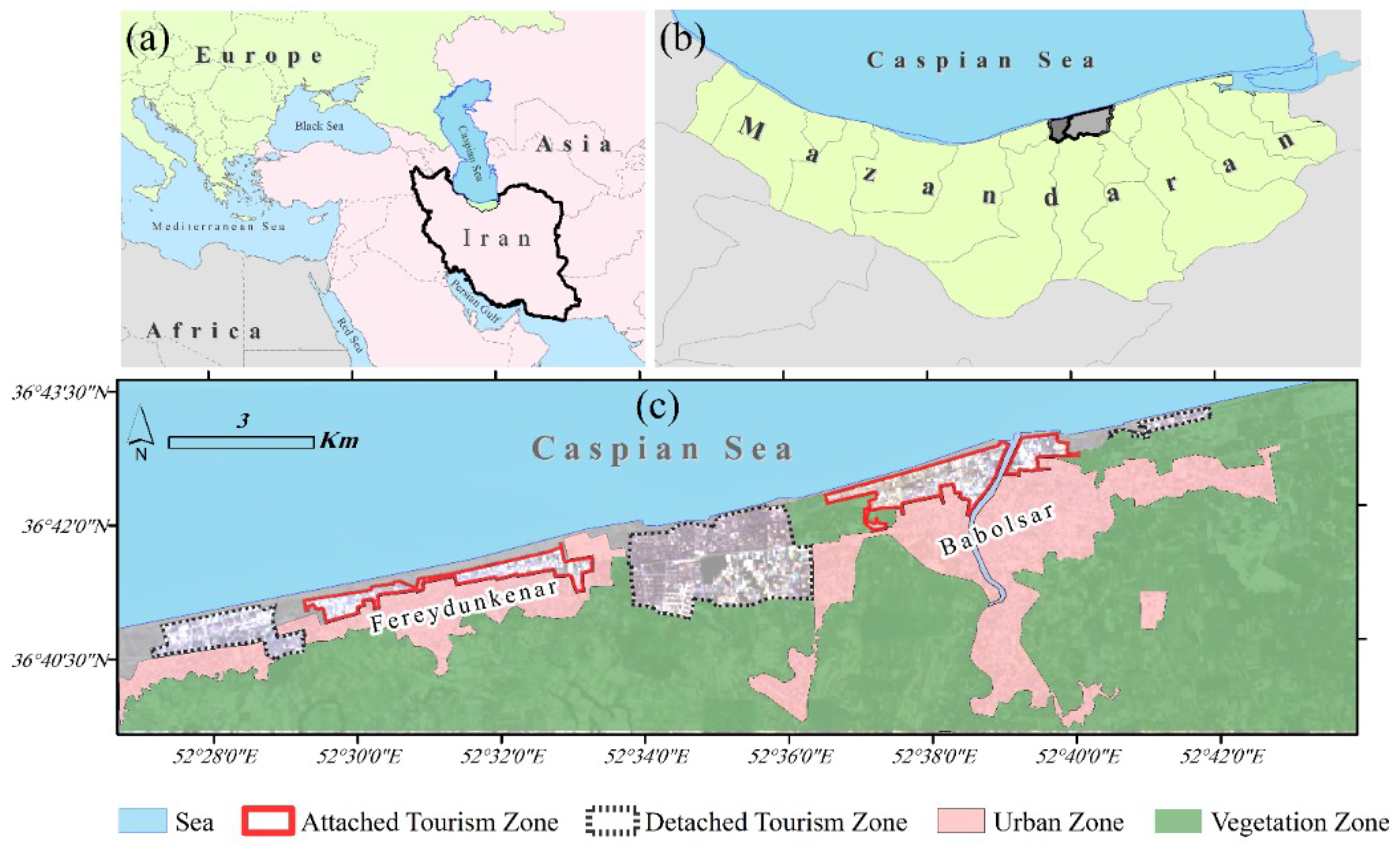
2.1. Study Area

The study area (Figure 1), the coastal cities of Babolsar, Fereydonkenar and their hinterlands, are located in Mazandaran Province, in the North of Iran and South of the Caspian Sea. These cities, with a population of about 100,000 people [73], have been one of the most popular domestic tourism destination in Iran for the past 50 years due to their proximity to the Caspian Sea, their well-developed tourism services and their hospitable communities. According to the results of a survey in Mazandaran Province, Babolsar is the second most attractive destination for domestic tourism after Ramsar [74,75]. As coastal cities with agricultural hinterlands, they have experienced increasing demand for tourism over recent decades. According to survey estimates, the area was the destination for nearly six million domestic tourists in 2017 [74]. The most important attractions in this area according to the survey are the sea, the climate and the variety and abundance of shopping centers. Using important climatic parameters such as temperature, relative humidity, wind, radiation and bio-climatic indicators presented by Baker et al., the climatic features of Babolsar and Fereydoonkenar show that, from May to November, Babolsar has optimal natural conditions for tourist activities in open space in terms of thermal comfort. Although in the two months of July and August due to the relative increase of temperature and high relative humidity, a sultry state prevails in these cities, the wind blowing, especially in the coastal area, make this situation tolerable and even optimal [76].
The growing trend of tourism in the study area over the past ten years has been such that the area has changed from a mostly agricultural area to a multi-functional area focusing on tourism and university education services [74].
The growth of tourism in the area in the two main forms of overnight stay and second homes has led to significant spatial changes. Tourism-induced spatial changes are mainly caused by the change of the coastal areas and bare land into second homes, shopping malls, hotels, restaurants, entertainment centers, urban public spaces and development of infrastructure such as roads, water and electricity [74].
Before addressing the effects of tourism in the study area, it is important to describe the main types of tourism development. As mentioned earlier, Babolsar and Fereydonkenar have two main types of tourism, overnight tourists and second home tourists. The main services to the overnight tourists have been developed in the coastal zone of the area, including hotels, inns, restaurants, shopping and entertainment centers. However, second home tourists are divided into two different categories, detached second homes, and attached second homes. The detached second homes have been developed mainly in the western wards of Babolsar, detached from the main urban area; their main feature is low density as well as vast yards and green space. In contrast, the attached second homes with higher density have been developed in the northern area and are attached to the urban zone.

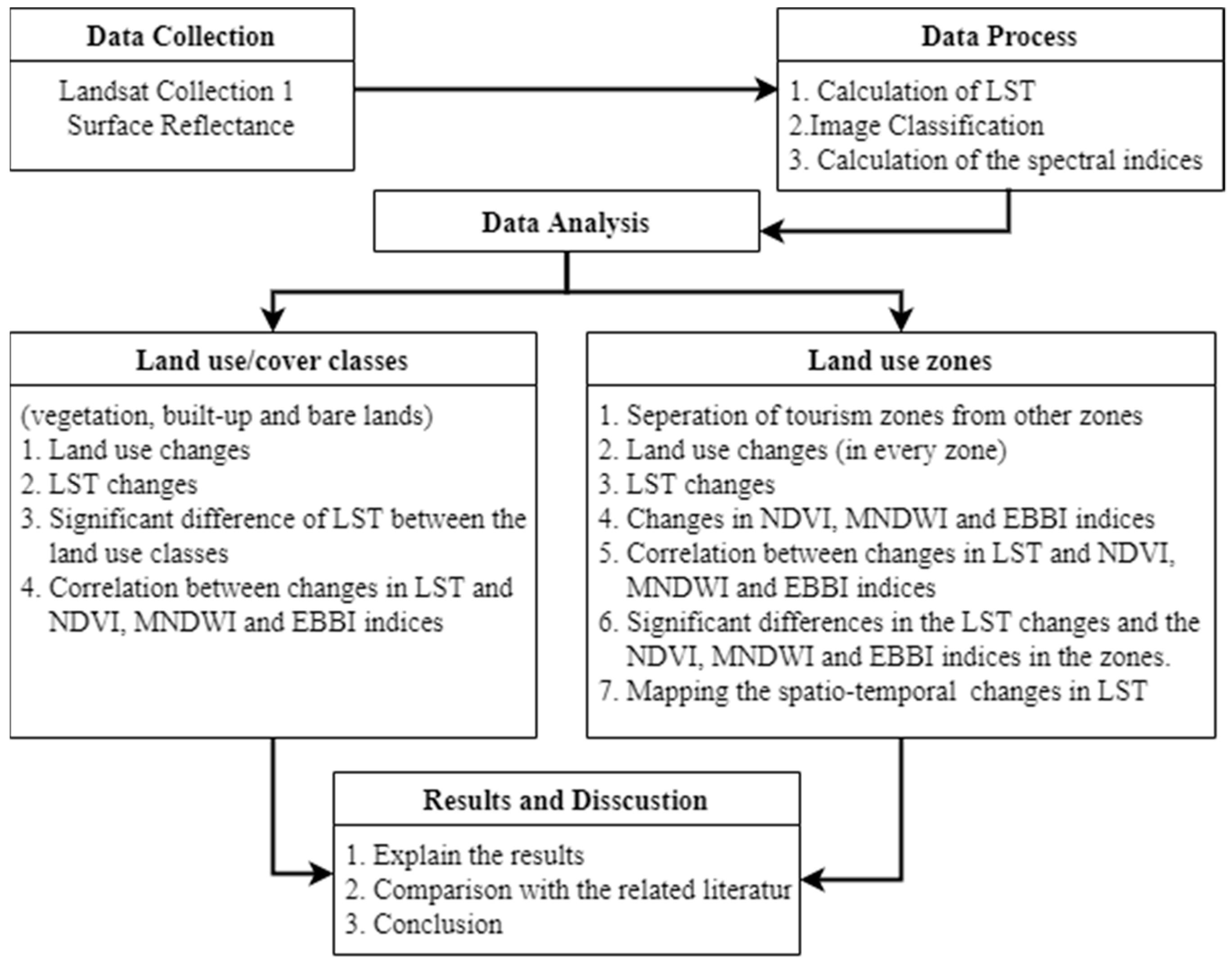
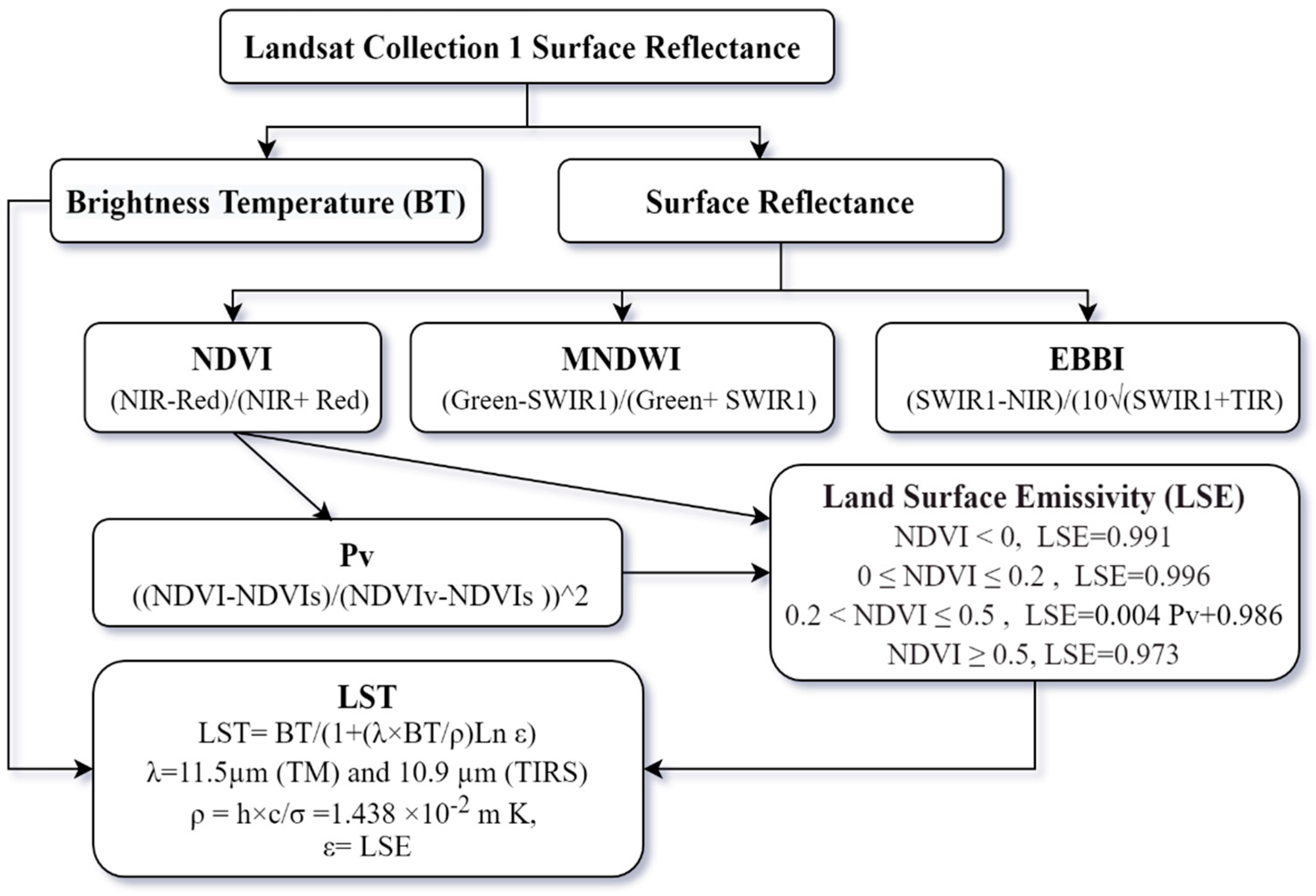
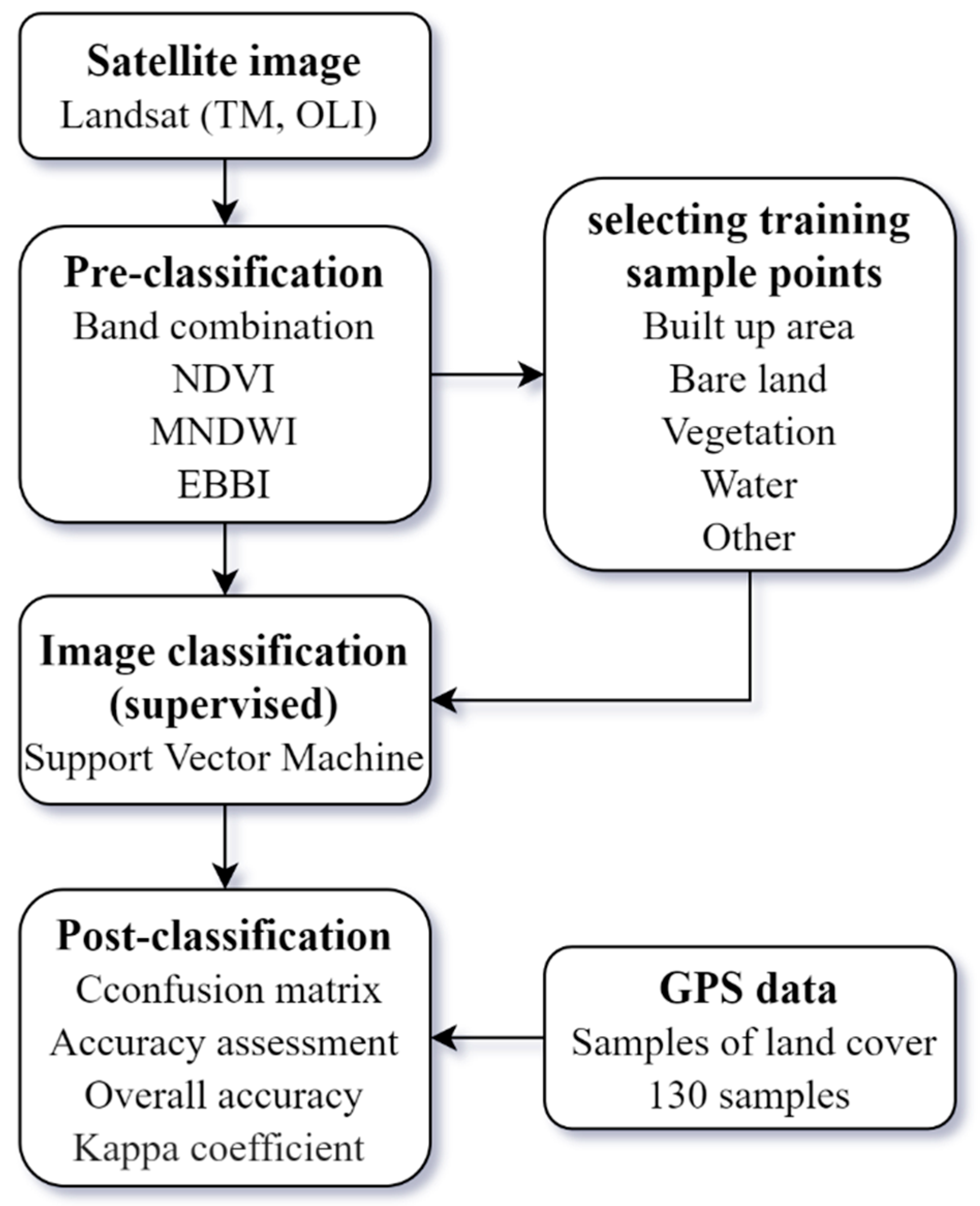
2.2. Data and Methods

In this research, the relationship between the spatial changes in tourism and changes in LST has been investigated using remote sensing techniques (Figure 2). It should be noted that all the analyses related to the land use/cover and LST changes were done during 32 years and in 6 periods, i.e., in the years 1987, 1993, 1999, 2009, 2014 and 2019 (Table 1).
To classify the images and calculate the main spectral indices and LST (Figure 3), the data were obtained from Landsat Collection 1 SR images taken in June and August (Table 1). SR improves comparison between multiple images taken from the same area by considering atmospheric effects such as aerosol scattering and thin clouds. This can significantly contribute to the detection and characterization of the land surface change [77,78]. In addition, the images have been selected carefully to observe two important points: (1) images with the least cloudiness and (2) images belonging to summer, because in this season the study area has the least cloudiness and the vegetation of the region is in its optimal condition in terms of components affecting growth (temperature and humidity). According to the physical characteristics of the area, all the land uses/cover was classified into three main categories: vegetation, built-up and bare lands.
Based on the reflectance characteristics and the NDVI, MNDWI, EBBI as well as the LST indices, the satellite images of the study area were finally classified (Figure 4). In this regard, first, the educational points with suitable distribution were selected for three main land use/cover classes (built-up, bare land, vegetation). For this purpose, as shown in Table 2, the MNDWI, NDVI and EBBI spectral indices were used to identify the training points of water bodies, vegetation, built-up and bare lands, respectively [78,79,80]. Then, the satellite images were classified using a supervised classification method and Support Vector Machine (SVM) Algorithm. The results of the classifications were evaluated using 130 well-distributed land sampling points based on the images belonging to the year 2019 (Figure 3). In this regard, the overall accuracy and kappa coefficient were obtained and the results confirmed the acceptable accuracy of the method used (overall accuracy = 96.07 and kappa coefficient = 0.93).
After identifying and classifying the various classes of land use/cover, the LST characteristics and its changes were studied separately for each land use class over the six time periods. Then, in order to investigate the probability of a significant difference between the 32-year averages of the LST of the three land use classes, vegetation, built-up and bare lands, one way ANOVA and Tukey technique were used. Moreover, to examine the relationship between the LST and the corresponding values of the NDVI, MNDWI and EBBI indices in each cell, Pearson correlation method was used for each year. In other words, the relationship between the type of land use/cover and the LST was investigated for each cell.
In order to investigate the relationship between the spatial changes in tourism and changes in the LST, first based on the 2019 images, the area of land uses related to the tourism sector, including second villa homes, second apartment homes and tourism services, were separated from the other land uses, especially urban spaces. Due to the relatively similar physical characteristics of the tourism and urban space, in order to separate these two zones two fieldwork steps were taken.
In the first step, eight real estate dealers and investment consultants with more than 10 years of experience in the area were selected using the snowball sampling technique and they were interviewed through open interview questions. The interviewees were asked to separate tourism spaces from the urban space according to their experience and in accordance with the map (Scale = 1:10,000). In order to verify the opinion of the real estate consultants, they were also asked about the address of the streets separating the tourism blocks. As mentioned, the development pattern of second homes in the study area includes second villa homes detached from the urban area and second apartment homes attached to the urban area. Thus, during the interview process, the two spaces were separated from each other. The experience and high mastery of real estate consultants, who even participated in many tourism projects in the region, provided the research team with accurate information on identifying areas for tourism development and their historical trends.
After receiving the views of the real estate consultants and confirmatory opinions from the last interviewed consultants, in order to control and verify the interviewees’ ideas, the plotted areas were re-examined by the research team. In the study area, it was relatively easy to distinguish second homes from native urban wards since the first preference of tourists is not to interfere with the native urban wards. Therefore, tourism spaces are separated from the native spaces using the streets as borders and sometimes fencing. On the other hand, the architecture of tourism spaces with the characteristic of more durable materials, modern design, use of new technology in construction and greater area, can be distinguished from the main urban wards. At the same time, in the case of blocks in which there was some interference between the urban and tourism spaces, if more than 70% of the land use in the block was dedicated to tourism activities or second homes, then that block would be included in the tourism zone. It is noteworthy that only a few blocks had this condition. However, due to the considerable physical distance from the main urban area, fencing and even the presence of security at the entrances, the identification of the detached tourism zone was made with great care, relying on the opinion of real estate consultants and field examinations. At the end of this stage, a vector border layer was created for all land uses in the form of four main zones: the urban zone, vegetation zone, detached second home zone (detached from urban area) and attached second home zone (attached to urban zone). This vector layer was used to analyze all pixels along with the LST values and land use characteristics in the next steps.
The area of different land use/cover classes (vegetation, built-up and bare lands) and LST were re-calculated separately for each of the four main zones (urban zone, vegetation zone, detached second home zone and attached second home zone). These calculations were repeated for all six time periods to obtain land use/cover changes in each zone over time. Thus, for each image pixel, the values related to the land use class, zone name, values of each of the NDVI, MNDWI and EBBI indices and finally the LST were recorded. Since Landsat images were presented in 30-m pixels (thermal images were also resized with 30-m pixels), the study area included 207,870 pixels. The values of each pixel were recorded in a table for statistical analysis. Thus, it was possible to run statistical analyses on the LST value and its relationship with the spectral indices at the level of each pixel, separately for the four main zones.
In order to calculate the rate of land use change from 1987–2019 for each zone, the following formula was used:
  Change   Rate = ( Class   Area 2019 Class   Area 1987 ) Class   Area 1987
where Change Rate indicates the rate of change; Class Area2019 indicates the area of land use class in 2019 at the related zone; Class Area1987 indicates the area of land use class in 1987 at the related zone.
The linear trend (α) formula presented below was also used to calculate the annual rate of change of the NDVI, MNDWI, EBBI and LST time series for each pixel.
y = αx + β
α = n x y ( x y ) n x 2 ( x ) 2
where α is the slope of the line, β is a constant, n is the number of years, y indicates the numerical value of the indices and the LST and x indicates the years studied.
After calculating the annual rate of change of the NDVI, MNDWI, EBBI and LST at the level of each cell separately for the four main zones, Pearson correlation coefficient was used to investigate the relationship between the LST changes and changes in the spectral indices. The purpose of this stage was to investigate in more detail the effect of spatial changes in tourism on changes in the LST. To further clarify this issue, one-way ANOVA and Tukey technique were used to investigate the significant differences in the LST changes and the NDVI, MNDWI and EBBI indices in the four main zones. The results of this section helped the researchers to investigate the effect of the spatial changes in the attached and detached tourism zones on changes in the spectral indices and the LST, and compare the results with the effect of the spatial changes in the urban zone and vegetation zone.
In addition to statistical analysis, according to the relationship between the mean and standard deviation of the annual change rate, the spatial and temporal patterns of the LST changes in the study area were divided into three categories: usual temperature changes, unusually high or low temperature changes, very unusually high or low temperature changes. In this regard, the values between X ± σ were considered as usual changes, values greater than X + σ and smaller than X + 2σ were considered as unusually high changes and values greater than X + 2σ were considered as very unusually high changes. On the other hand, values smaller than X − σ and greater than X − 2σ were considered as unusually low changes and values smaller than X − 2σ were considered as very unusually low changes.

3. Results

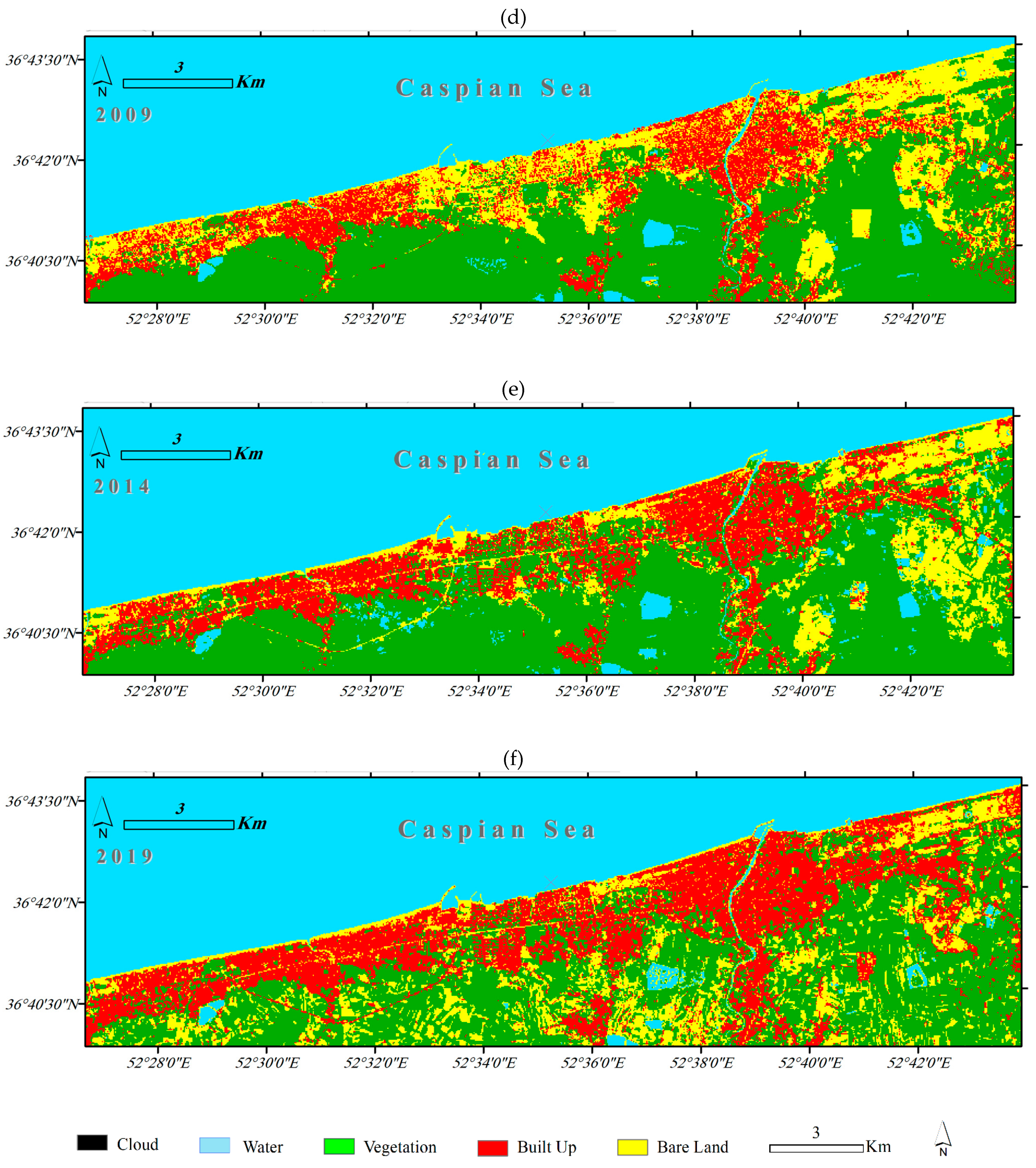
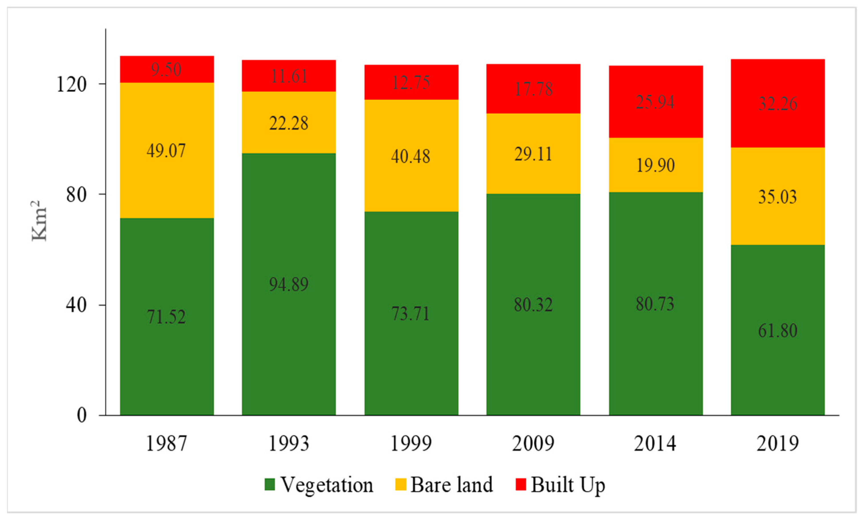
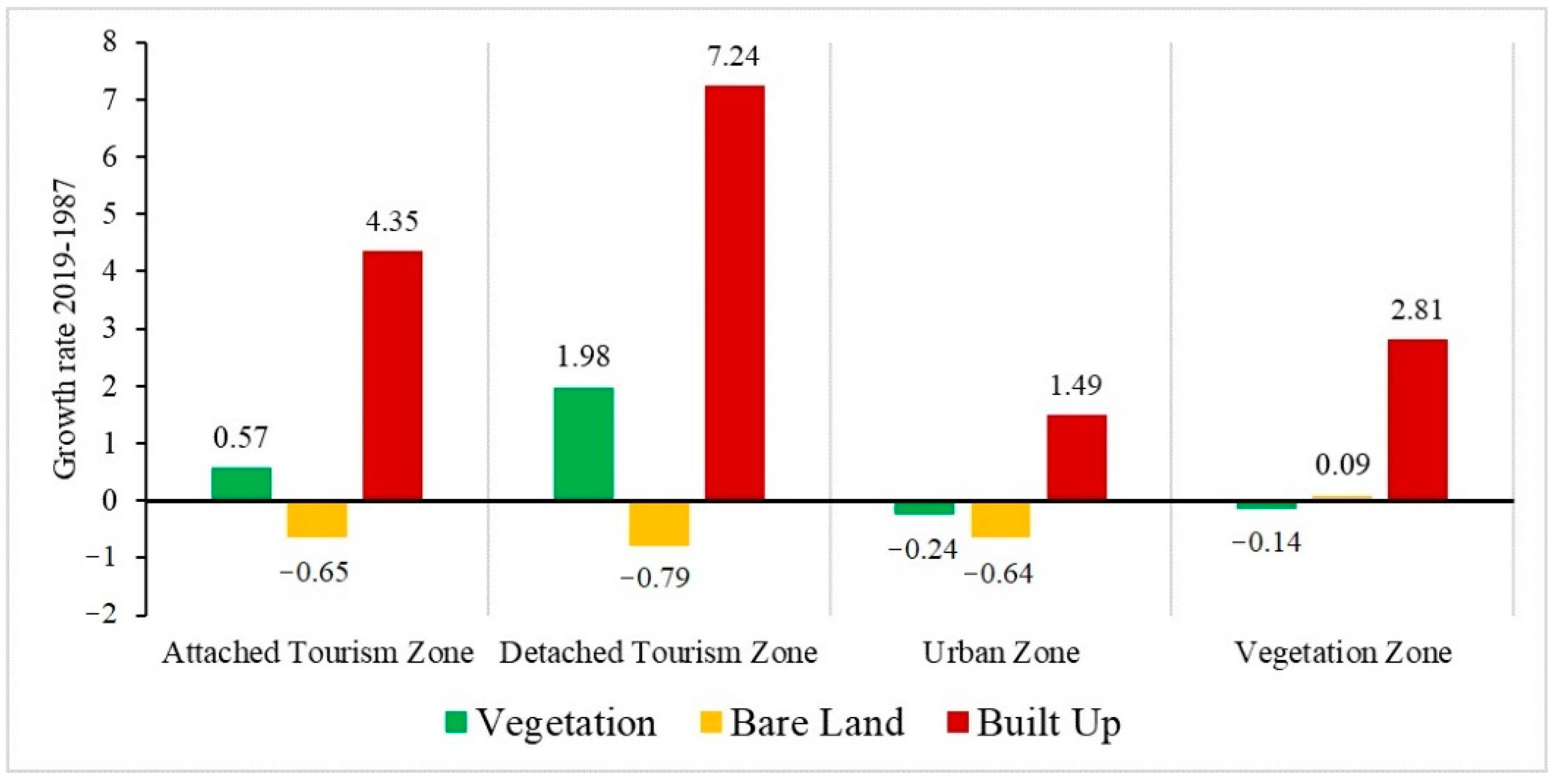
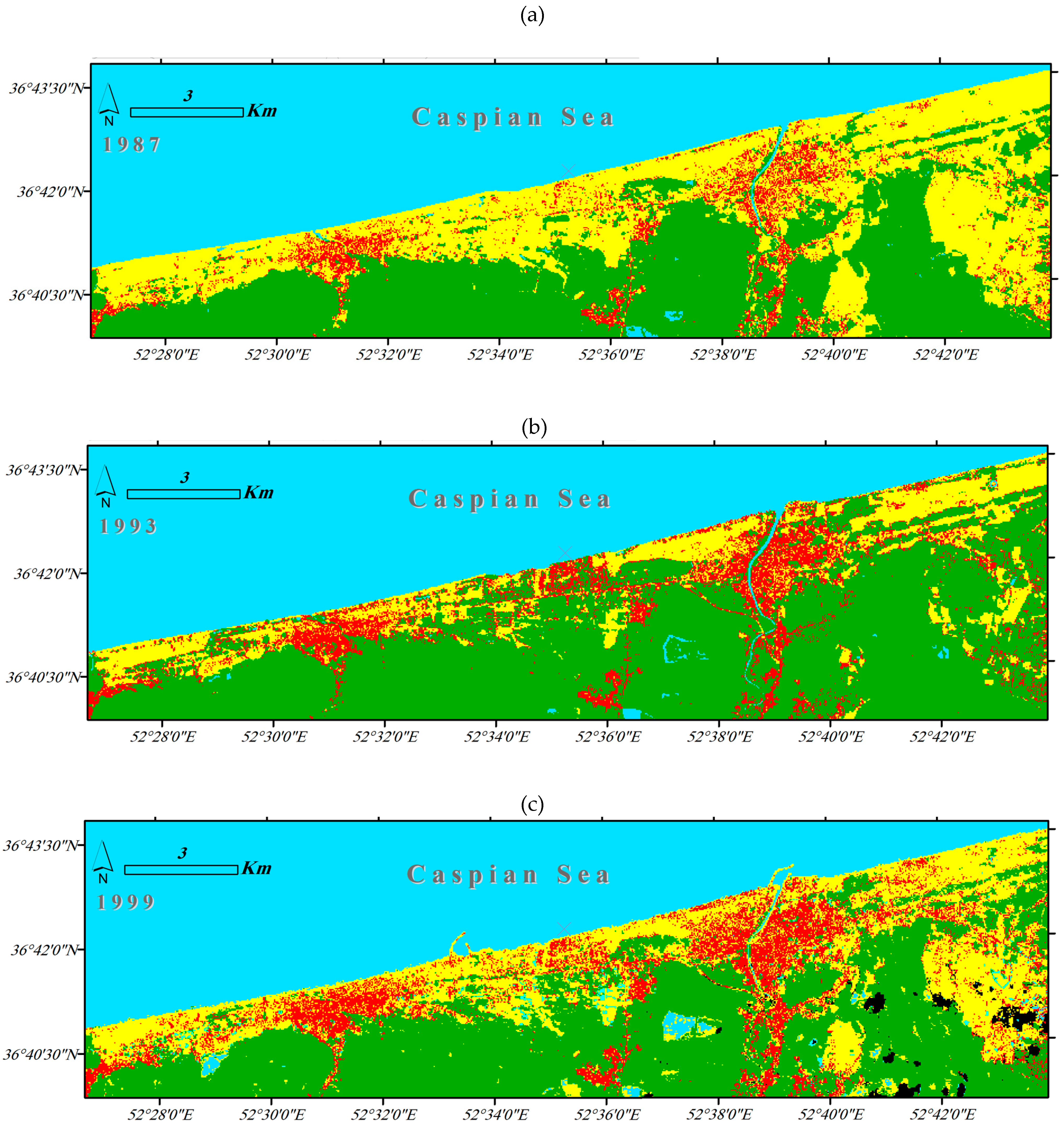
3.1. Land Use Changes in the Study Area

In this study, in order to investigate the possible impact of tourism on changes in the LST, first land use changes in the area were analyzed over a period of 32 years (in six time periods) from 1987 to 2019. In this regard, first the land use/cover changes in the area were analyzed in three classes, i.e., built-up, bare lands and vegetation, and then, by separating the area of tourism spaces from other land uses, the effect of the spatial changes in tourism on land use changes and changes in the LST were examined.After the easing of economic and security unrest caused by the Iran–Iraq war, from 1987 onwards the entry of domestic tourists, both as overnight and second-home tourists, gradually increased in study area [74]. In the development process of tourism spaces, proximity to the coastal area and relative distance from native settlements have been the criteria for investors of second homes and tourism services [74]. On the other hand, due to the relative salinity (unsuitable for agriculture), first bare lands with a suitable location were transformed into projects for the construction of second home complexes and tourism services. Between 1987 and 2019, the area of bare land decreased from 49 to 35 km2 with a negative annual change rate of 2.53 km2. Vegetation coverage also decreased with a negative annual change rate of 2.41 km2, while the area of built-up land use increased with an annual change rate of 4.62 km2 from 9.5 to 32.26 km2. This shows that the area of built-up land use has increased by about 340% from 1987 to 2019 (Figure 5 and Figure 6).

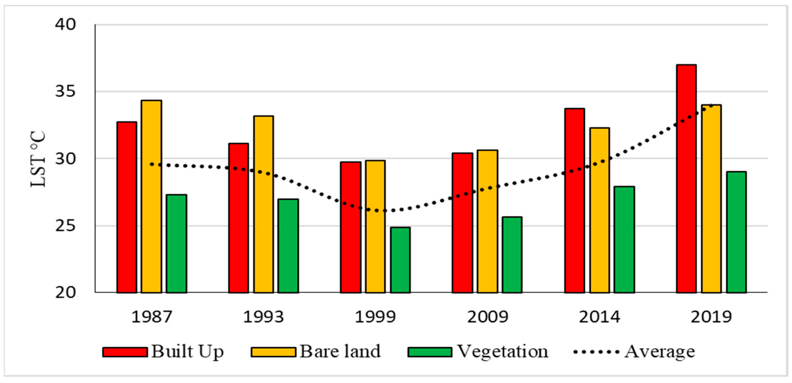
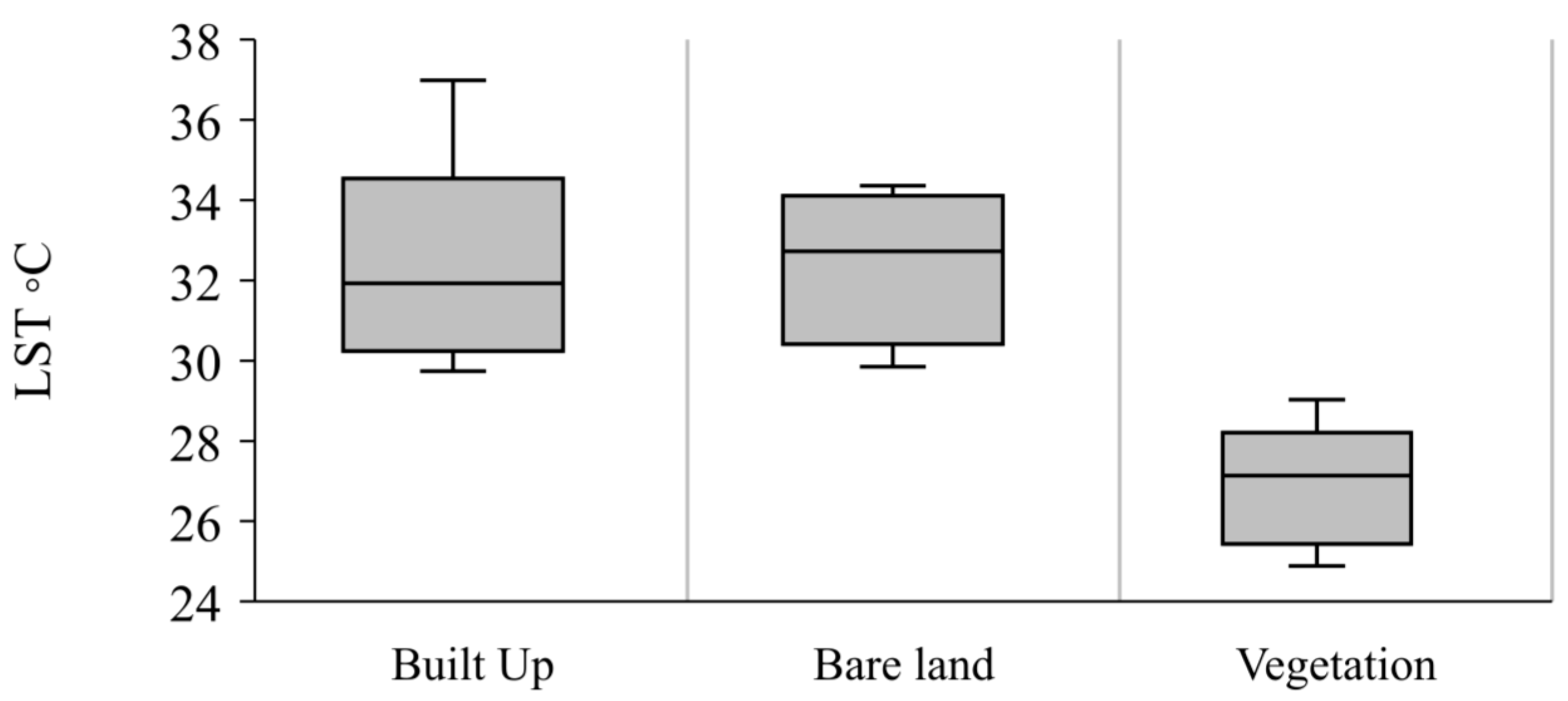
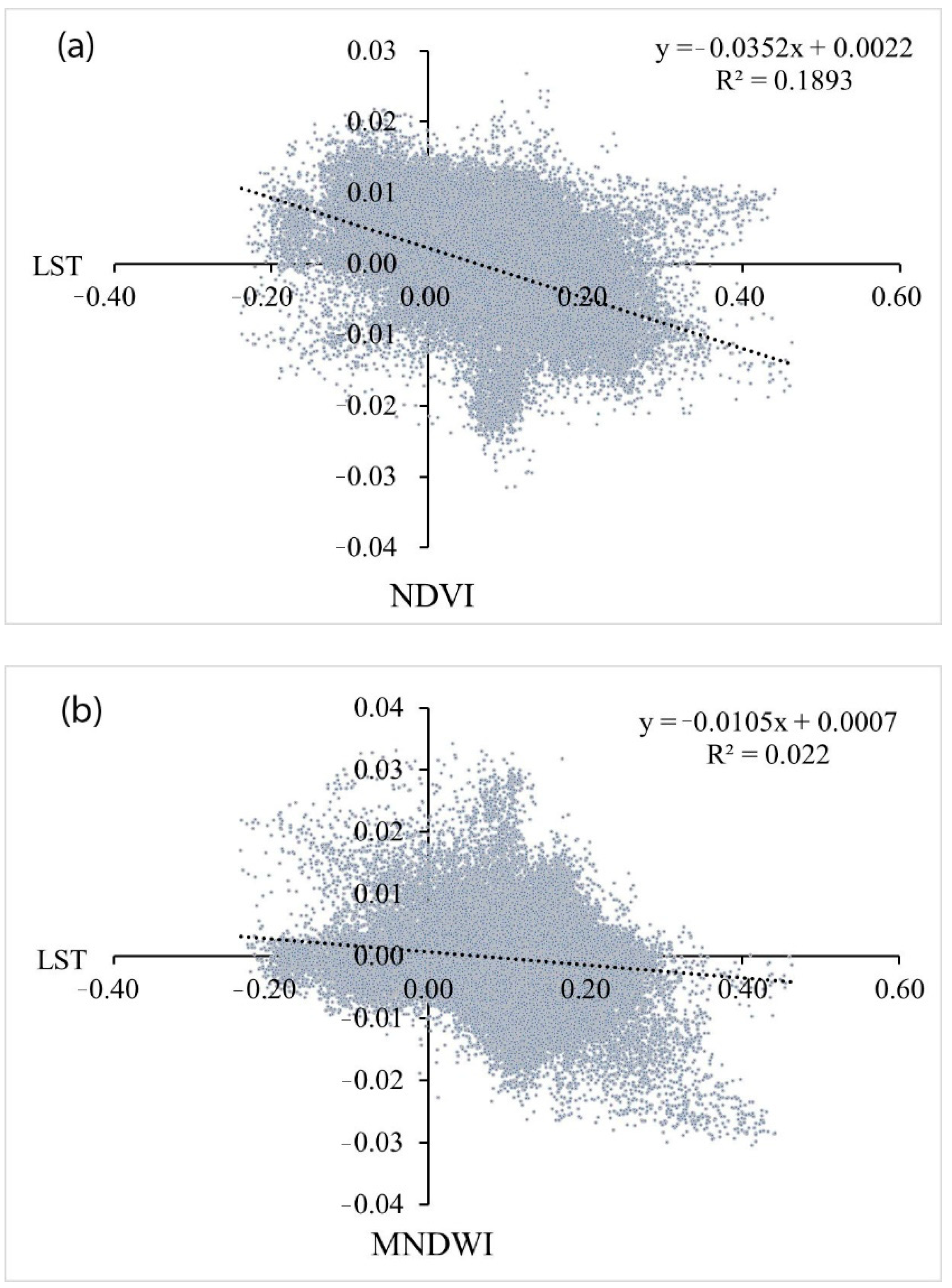
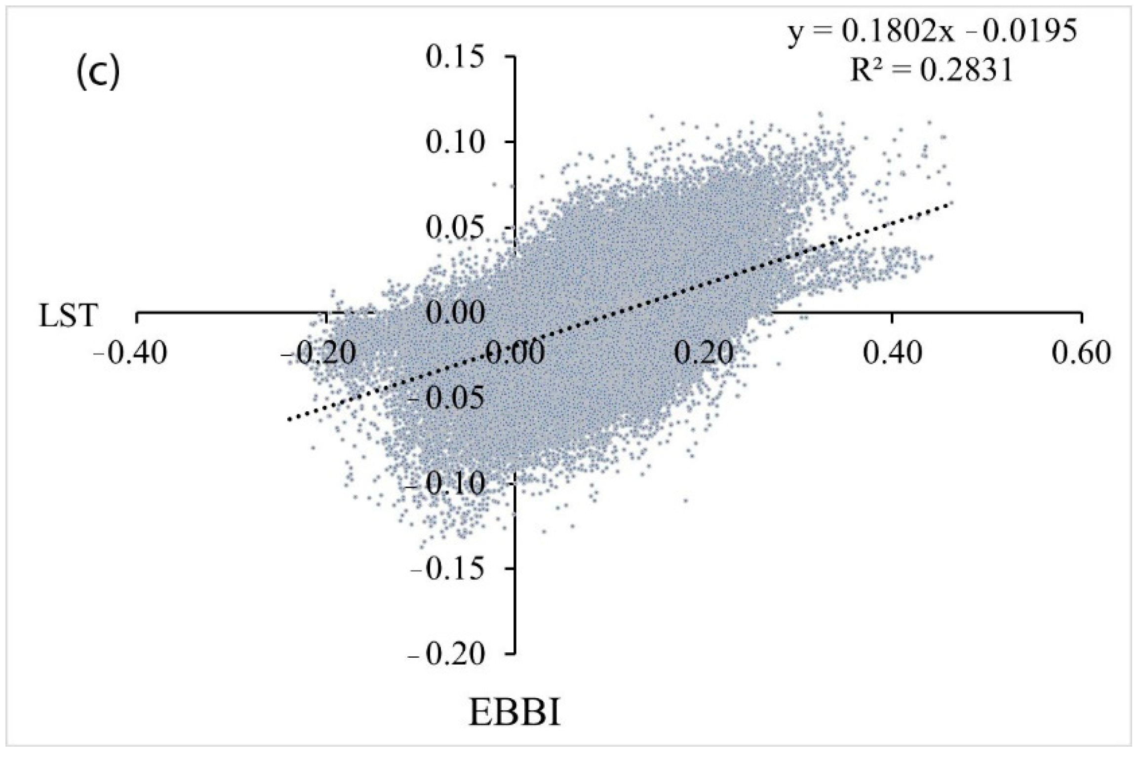
3.2. The Impact of Land Use Changes on LST Changes

At this stage of the research, to investigate the relationship between the land use/cover and the LST, the LST changes associated with each of the land use classes (built-up, bare land and vegetation) were examined for six time periods from 1987 to 2019 (32 years). For this purpose, first the six-period average of the LST was calculated separately for each pixel and then the results were compared based on the three main land use classes. The results show that, in general, the average LST of all land use classes displayed a decreasing trend from 1987 to 1999. However, from 1999 to 2019, they increased. In the meantime, due to shading and evapotranspiration processes, the vegetation class has been cooler in all the years under study with a difference of 5 °C between the built-up and bare lands (Figure 7 and Figure 8).
The results of ANOVA test showed that there was a statistically significant difference between the mean of the LST of the studied land use classes (1987–2019) (F = 14.033, p < 0.0001). In a more detailed investigation, the results of the Tukey HSD test also showed that the LST values in the vegetation class significantly differed (difference ≃ 5.5 °C) from the LST in the bare lands and built-up area during the six periods studied (p = 0.001). However, this difference was insignificant between the bare lands and the built-up area (p = 0.998) (Table 3 and Table 4). In this regard, the highest values of the LST were observed in the bare lands in 1987 and 1999, while in 2014 and 2019 the built-up lands had the highest LST values (Figure 7). The bare lands became warmer in 1987 and 1999 due to their sand cover, which had to support construction in the following years, with the development of tourism, especially in the coastal lands. At the same time, a large part of the bare lands identified in the images of 2014 and 2019 were related to farmlands. The crops were harvested earlier than planned due to the earlier start of the hot season.
As described in the research method section, in the next stage the correlation between the LST values and the corresponding values of the NDVI, MNDWI and EBBI indices were calculated at the pixel level (Table 5). The results of this stage showed that, in all the six time periods studied, there was a direct and significant correlation between the LST and EBBI index, indicating that the LST increases with increases in built-up and bare land areas. Due to the decrease of bare land area during the studied periods, it can be found that the positive correlation between the LST and EBBI is mainly due to the built-up area expansion. In contrast, the results showed that there is a significant inverse relationship between the LST and the NDVI and MNDWI indices, which indicate the vegetation and water bodies, respectively.
This study shows that the correlation between the LST and NDVI changed from −0.4 in 1999 to −0.79 in 1987. The correlation values of these two variables during the six time periods studied show a significant inverse correlation. In contrast, the correlation between the LST and EBBI was significant and direct, so that in all the six time periods studied, the correlation between these two variables was at least from 0.69 to 0.88.

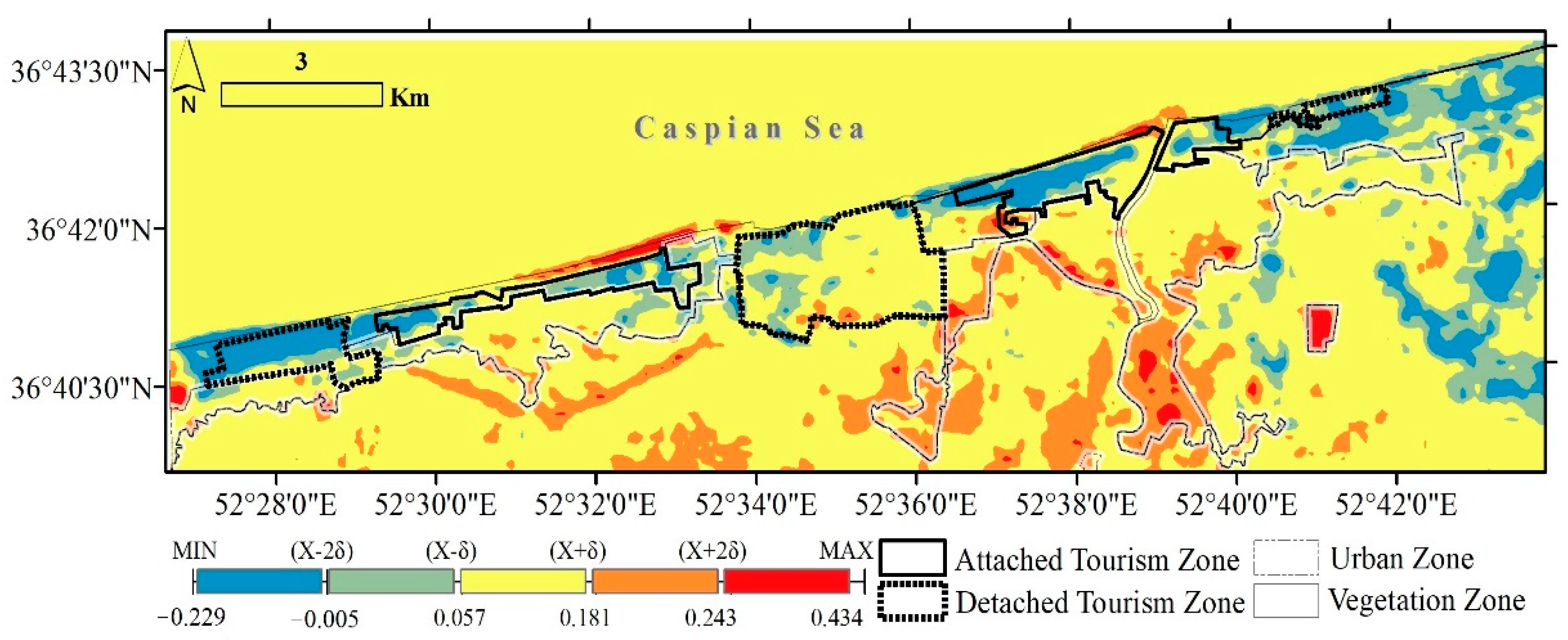
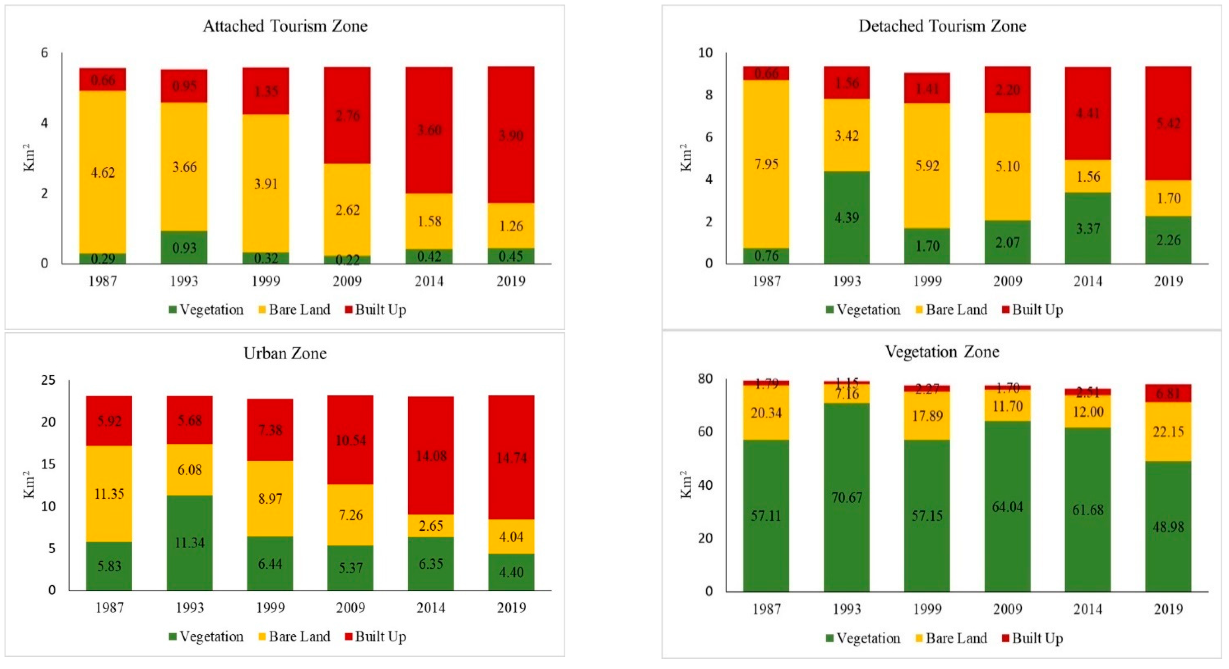
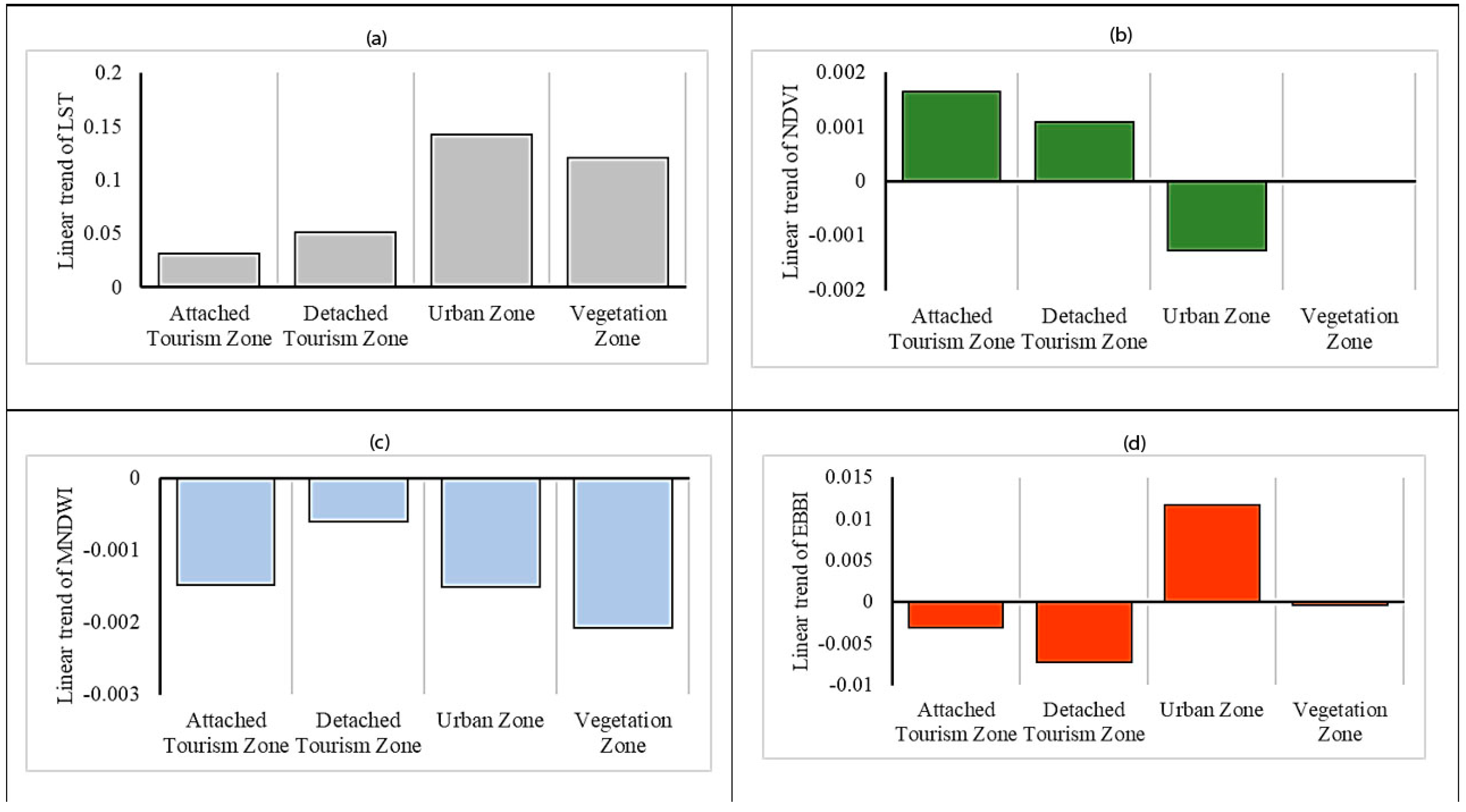
3.3. The Impact of Tourism Spatial Changes on LST

To investigate the effects of spatial development in tourism on the LST, the whole study area was divided into four zones including the urban zone, vegetation zone, the second home zone detached from the urban zone (with all surrounding tourism services), and the second home zone attached to the urban zone based on the images of 2019 (research method section). By separating the tourism areas, it was possible to study the impact of tourism on the spatial changes of the region and finally on the changes of the LST. Findings show that the built-up area in the two tourism zones increased from 1.32 km2 to 9.32 km2 from 1987 to 2019. Compared to the total built-up area in the region in these two years, tourism zones made up 14.57% and 30.18%, respectively. On the other hand, the built-up area in the urban zone increased from 5.92 to 14.74 km2 from 1987 to 2019 which made up 65.59% and 47.74% of the total built-up area in the region, respectively. In other words, the built-up area in the two tourism zones increased by 708.1% from 1987 to 2019, while this increase was 248.8% in the urban zone. Therefore, the expansion of the built-up area in the tourism zones was more than 2.5 times as much as in the urban zone. This indicates the role of tourism in the occurrence of significant spatial changes in the study area (Table 6).
In addition, the 32-year changes in the three classes of land use/cover, built-up, bare land and vegetation, in each of the four zones revealed more detailed information about the spatial changes within each zone (Figure 9 and Figure 10). Findings show that the area of bare land in the attached tourism zone, with an annual change rate of −0.65, decreased from 4.62 km2 in 1987 to 1.26 km, while in the detached tourism zone the annual change rate was −0.79. In contrast, the area of vegetation coverage in the two tourism zones increased. The vegetation area in the detached tourism zone increased by an annual growth rate of 1.98, from 0.76 km2 in 1987 to 2.26 km2 (Figure 9).
In this stage of the research, in order to distinguish the effects of tourism on LST from other land uses, paired comparisons were made between the main zones. In this regard, first the correlation between the annual change rate of the LST and the annual change rate of the NDVI, MNDWI and EBBI indices was calculated in the studied zones during the six time periods (from 1987 to 2019) (Table 7). The results of the Pearson correlation test show that there was a significant direct relationship between the trend of changes in the LST and the trend of changes in the EBBI index. However, this relationship was inverse in the trend of changes in the NDVI and MNDWI indices. This shows that the rising trend of the LST is directly related to the expansion of built-up and bare lands. In contrast, in areas with increasing vegetation and water body, the LST tended to decrease over the 32-year period (Table 7 and Figure 11).
In the next step, using an ANOVA statistical test, the trend of changes in the LST and NDVI, MNDWI and EBBI indices were compared statistically between the main zones in the area. The results showed that the 32-year trend in changes in the LST was significantly different in all four main zones, with 95% confidence. This result is also true for the trend of changes in the spectral indices (Table 8 and Figure 12).
The results show that the trend in annual changes in the LST is increasing in the whole study area, but its values show a significant difference between the main zones, so that the increasing trend of the LST in the urban and vegetation zones was higher than that of the tourism zones. This indicates that the nature of spatial development of tourism, although seemingly similar to the nature of urban development, has an inverse effect on the LST in the tourism zones. It is noteworthy that the record of higher LST in the vegetation zone, which mainly includes farmlands, is due to the bareness of these lands after harvest at the time of study. Therefore, the result of the analysis of the above statistical test on the difference in the LST of the vegetation zone and tourism zones is invalid.
At the beginning of the research, with the aim of investigating the effect of tourism on the LST in more detail, two separate tourism zones were selected, as attached to and detached from the urban area. Thus, if the results are mixed with the urban zone, it is possible to separate these two types of tourism development model. Although the results of the paired comparisons show a significant difference in the changes in the LST and the spectral indices between the two tourism zones, a comparison of the results of the Tukey test makes it clear that both tourism zones have a different effect from that of the urban zone on changes in the LST. By examining the impact of tourism on the spectral indices (Table 9), the reason for this difference becomes clear.
According to what has been said, tourism has moderated the LST in tourism zones both through the development of sandy bare lands and the development of green spaces (increase of the NDVI index). In contrast, in the urban zone, the NDVI index with a negative change rate and the EBBI index with a higher positive change rate show a significant difference to the tourism zone. In contrast to tourism development, the urban development model had a higher EBBI rate on the one hand, and on the other hand the development of the urban zone on the agricultural lands and the neglect of green space development has caused a continuous decrease in the NDVI index. Therefore, during the study period, the LST of the urban zone has always been higher than that of the tourism zones.
In the following, in addition to the above-mentioned statistical tests, first, the annual trend of the LST changes in the whole area was calculated (at the pixel level) to depict the spatial pattern of 32-year changes in the LST, and then the distribution pattern of the usual/unusual and very unusual values was shown (research method section). By adapting the boundaries of the four main zones with their trend values, the majority of pixels with very unusually low and unusually low values trend belonged to the tourism zones. This result shows that, during the 32-year period, with the development of tourism spaces on bare lands and the development of green spaces in the tourism areas, the LST experienced a declining trend with a significant difference from the other zones. In contrast, the majority of pixels with a very unusually high value (warmer) were seen in the urban zone (Figure 13).
A more detailed study of the spatiotemporal pattern of the trend in LST changes in the study area shows that the pixels with the usual change value had a LST change between 0.057 to 0.181 °C per year. Peng et al. [85] also reported similar amounts of long-term LST change as usual in a study on Chinese cities.
In the study area, most of the pixels with usual LST changes included parcels with no land use change during the 32-year period, and therefore it can be said that they have become warmer in line with global warming. In contrast, pixels with unusually high and very unusually high (warmer) changes were divided into two groups. The first group included parcels with vegetation cover that went under construction between 1987 and 2019. These areas included parcels integrated in the urban zone or parcels with changed land use as a result of the development of infrastructures, e.g., Fereydonkenar ring road. Other pixels with unusually high LST changes included infrastructure development projects such as ports, piers, and offshore access routes (in the north at the coastal line) that have created new built-up areas inside the sea.
There were two areas with unusually and very unusually low (colder) LST changes. The first area includes bare lands which changed to vegetation coverage during the study period. These areas mainly included agricultural lands located in the east and southeast of Babolsar. The second area was located in the tourism zones (detached and attached zones). The bare lands in these zones were used for tourism-related infrastructure. These constructions included second homes, green space in the tourism zone, shopping and recreation centers. This finding is further evidence for the significant impact of spatial changes in tourism on changes in the LST.

4. Discussion

The main results of this study showed that tourism, especially second homes, over a period of almost 30 years, as a strong driving force, has caused widespread land use change in the study area. As a result, the spatial changes caused by the development of tourism, in subsequent years, have caused significant changes in the LST of the region.
Previous research has repeatedly shown that the amount of outgoing energy (Albedo and Outgoing Longwave radiation (OLR)) is strongly influenced by the physical characteristics of the land surface. Thus, any change in land surface characteristics will lead to changes in the properties of radiation and ultimately changes in temperature [35,36,37,38,39,86,87,88,89,90,91,92,93,94,95,96,97,98,99,100,101,102,103,104,105,106,107,108,109,110]. In this regard, the LST has been considered as an important indicator in environmental studies [93].
In this study, the results of the ANOVA test showed the significant effect of three main land use/land cover classes, including built-up, bare land and vegetation on the LST. Accordingly, due to evapotranspiration and shading processes, vegetation has a significant effect in reducing the LST by 5 °C. The results of the correlation test also confirmed a significant inverse relationship between the LST and NDVI and MNDWI indices. The correlation between the LST and NDVI during the six study periods also showed a strong relationship from −0.4 to −0.79. A review of similar research also shows that, first, the relationship between the LST and NDVI is significant and inverse. The value of this correlation has been reported to be −0.4 and more [100,101,107,110]. In contrast, the correlation between the LST and EBBI was significant and direct, so that in all six time periods studied, the correlation between these two variables was from at least 0.69 to 0.88. Peng et al. [85] have also confirmed such a strong correlation between these two variables in their research.
This result shows that the LST has increased with increases in the area of built-up and bare lands, while increasing the area of vegetation and water bodies has reduced the LST in the study area. These particular results is in line with previous research showing the significant effect of vegetation on the LST [37,100,101,102,103,104,105,106,107,108,109,110]. In this regard, Rahman et al. [97], by modeling the spatial changes in the coastal lands and their effects on the LST characteristics, showed that physical changes due to urban development and built-up lands have a direct and significant effect on the LST, and this could pose a challenge for the residents of the studied areas in the future. The warmer built-up surfaces and the moderating role of vegetation on the LST were also confirmed in this study. Hellings et al. [99] referred to the impact of urban development and built-up space on increasing the LST in European cities, showing that green spaces and vegetation coverage reduce the LST by between 4 to 6 °C compared to built-up spaces and impermeable urban surfaces. The results of the study by Maheng et al. [37] of the city of Colombo in Sri Lanka show that a 30% increase in green space in a built-up urban environment moderates the average air temperature by 0.1 °C. In contrast, changing the use of suburban vegetation to urban spaces will increase the average temperature from 27.73 to 27.75 °C. Although this research has been carried out in different geographical conditions, its results are in line with the results of research from major European cities [99], Sri Lanka [37] and Indonesia [39] with temperate climates, showing a significant effect of vegetation in decreasing the surface temperature in different climates.
In this study, more detailed results were obtained by separating the tourism zone from the urban zone and vegetation. Unlike urban development models, the tourism development model in the study area has occurred in such a way that it did not increase the LST, but moderated it. The results of ANOVA and Tukey tests showed that there is a significant difference between tourism zones and other zones based on the LST, NDVI, MNDWI and EBBI indices, so that during the 32-year period, the tourism zones showed higher values of positive changes in the NDVI and MNDWI indices and lower values of changes in the EBBI index. This means that tourism in the study area has improved and has developed vegetation and water bodies in the tourism zones, but at the same time, the area of vegetation coverage has declined in the region. Therefore, the LST values in tourism zones have always been lower than in the other zones. This finding is fundamentally different from the findings of Chu et al. [94] in Hainan Island, China. By dividing the study area into two main zones, tourism and non-tourism, Chu et al. [94] showed that the development of tourism over a period of 20 years has a direct and significant effect on increasing the LST so that the average difference between the surface temperature of the tourism zone and other areas was more than 1.2 °C per year. The tourism development model in Hainan Island caused extensive destruction of vegetation in the region and replaced it with impermeable surfaces related to tourism structures. In contrast, the development of tourism in the Babolsar area, on the one hand, has occurred through the change in use of bare lands that have been covered with sand. Sandy surfaces, with lower specific heat capacity than built-up surfaces, have a greater effect on increasing the LST. Therefore, the development of bare lands to the built-up tourism spaces has led to a decrease in the LST. On the other hand, the development of tourism spaces in the area has led to the development of green spaces that are irrigated regularly (Figure 9 and Figure 12). One of the most important marketing strategies of tourism investors in the study area is the development of well-designed green spaces within tourism projects. Accordingly, although the goal of investors is mainly advertising and beautification of tourism areas, this measure has affected the microclimate of the tourism zone by reducing the LST. In this regard, Goldblatt et al. [107] conducted a study of microclimate on the campus scale, citing the relationship between the NDVI, NDBI and LST. They found that, in comparison with the physical characteristics of the bare and built-up lands, developed vegetation within a campus has a significant effect on cooling the LST.
The findings of this study showed that tourism with a specific physical development pattern can have a significant effect on changes in the LST. However, it cannot be argued confidently that tourism development reduces the LST because, as Chu et al. [94] in their research on Hainan Island showed, that the effect of tourism on the LST depends on its physical development pattern. In the case investigated in this study (Babolsar and Fereydonkenar), tourism had a significant moderating effect on the LST in the tourism zones through developing green spaces that were constantly irrigated, and constructing on bare lands that were generally covered with sand. Although this study focused on the effects of the physical development of tourism instead of urban development, its results on the correlation between the land cover indices such as NDVI, MNDWI and EBBI with the LST are consistent with previous research [92,93,94,95,96,97,98,99,100,101,102,103,104,105,106,107,108,109,110].
The findings of this study are significant because, at the beginning of the research, there was no similar study in the relevant literature and, so far, only one similar piece of research has been published [94]. This research has tried to deal with the relationship between the physical changes and changes in the LST from another perspective. On the other hand, a large part of the research related to the relationship between land use/cover characteristics and LST has been conducted in temperate and humid regions with rich vegetation, and relatively less research has been done in countries with arid climates such as Iran [96]. In this regard, providing evidence from different contexts will help to enrich the relevant literature. This research faces limitations, which can be addressed in future research. Although the temperature data and the related indices were analyzed in six time periods (32 years) on a pixel level from the whole area, they all belonged to a limited period of summer when the vegetation and cloud cover of the area were in optimal condition. Therefore, it would be useful to obtain more data covering the other times of the year to enrich the analysis, though this may increase the volume of data and input of the analysis. Therefore, other researchers could contribute to the enrichment of the relevant literature by providing new evidence through conducting a similar research over longer periods and in different climates, according to different patterns of tourism development.

5. Conclusions

This study investigated the possible effect of spatial changes in tourism on the LST. Although several studies have been conducted to investigate the effect of land use/cover changes on the LST, only one study has been published before this article on the effect of tourism. Thus, more evidence and different research conditions and methods are required. In this research, in order to classify the satellite images, the Landsat Collection 1 SR images taken in June and August were analyzed during 32 years in six periods, i.e., the years 1987, 1993, 1999, 2009, 2014 and 2019. In line with the purpose of the research in the first stage, the spatial changes and then the LST changes were studied in the area over a period of 32 years and in the six time periods mentioned above. Then, the correlation between the LST changes and the changes in the NDVI, MNDWI and EBBI indices was examined in the area. In the second stage, with the aim of analyzing the effects of tourism on changes in the LST, based on the field method, the whole area was divided into four main zones including the urban zone, the vegetation zone, the tourism zone attached to the urban area and the tourism zone detached from the urban area. Then, using the data belonging to the period of 32 years, the LST changes and its relationship with the NDVI, MNDWI and EBBI indices were calculated separately for each zone. Finally, the LST values and their relationship with the spectral indices were statistically compared between the four main zones.
The results showed that tourism over a period of 32 years (1987–2019), along with a significant change in land use/cover, has played an important role in the spatial changes of the study area. Similarly, the results confirmed the significant correlation of LST changes in tourism zones. The results showed that the nature of the effect of tourism on the LST is different from the other types of physical change factors, such as urbanization. This means that, in the study area, tourism did not increase the LST. Instead, cooler temperatures were always recorded in the tourism zones compared to the other land use/cover zones. By examining the reasons for this in more detail, the findings showed that the development of tourism in the area with the development of green spaces has helped to increase the NDVI index values. On the other hand, since the green spaces in the tourism zones were regularly irrigated, this has helped to further decrease the temperature. The development of tourism in the bare lands in the coastal areas is also another reason for this phenomenon. The bare lands in the tourism zones were mainly covered with sand, which increased the LST due to low specific heat capacity. However, the replacement of the mentioned land use with built-up area or green spaces has led to a decrease in the LST in the tourism zones. The findings of this study showed that the factors affecting the spatial changes such as urbanization and tourism cannot necessarily have similar effects on the environmental indices such as the LST. In addition, not all tourism development patterns can have the same effects. According to the results of this research, a tourism development model that leads to the development of green space can lead to lower LST in the area.

Author Contributions

Conceptualization, T.S., M.G., A.D. and M.P.; methodology T.S. and M.G.; software, T.S.; validation, T.S., M.G., A.D. and M.P.; formal analysis, T.S.; M.G.; investigation, M.P. and M.G.; resources, A.D.; data curation, T.S.; writing—original draft preparation, T.S., M.G.; writing—review and editing, T.S., M.G., A.D. and M.P.; supervision, A.D.; funding acquisition, A.D. All authors have read and agreed to the published version of the manuscript.

Funding

This research was funded by Alexander von Humboldt-Stiftung, grant number: 627 004 90.

Institutional Review Board Statement

Not applicable.

Informed Consent Statement

Not applicable.

Data Availability Statement

Not applicable.

Conflicts of Interest

The authors declare no conflict of interest.

References

  1. Berrittella, M.; Bigano, A.; Roson, R.; Tol, R.S. A general equilibrium analysis of climate change impacts on tourism. Tour. Manag. 2006, 27, 913–924. [Google Scholar] [CrossRef] [Green Version]
  2. Dogru, T.; Marchio, E.A.; Bulut, U.; Suess, C. Climate change: Vulnerability and resilience of tourism and the entire economy. Tour. Manag. 2019, 72, 292–305. [Google Scholar] [CrossRef]
  3. Lise, W.; Tol, R.S.J. Impact of climate on tourism demand. Clim. Chang. 2002, 55, 429–449. [Google Scholar] [CrossRef]
  4. Scott, D.; Hall, C.M.; Stefan, G. Tourism and Climate Change: Impacts, Adaptation and Mitigation; Routledg: London, UK, 2012. [Google Scholar]
  5. Scott, D.; Hall, C.M.; Gössling, S. A review of the IPCC Fifth Assessment and implications for tourism sector climate resilience and decarbonization. J. Sustain. Tour. 2016, 24, 8–30. [Google Scholar] [CrossRef]
  6. Scott, D.; Hall, C.M.; Gössling, S. Global tourism vulnerability to climate change. Ann. Tour. Res. 2019, 77, 49–61. [Google Scholar] [CrossRef]
  7. Gössling, S. Global environmental consequences of tourism. Glob. Environ. Chang. 2002, 12, 283–302. [Google Scholar] [CrossRef]
  8. Peeters, P.; Dubois, G. Tourism travel under climate change mitigation constraints. J. Transp. Geogr. 2010, 18, 447–457. [Google Scholar] [CrossRef]
  9. Zhang, J.; Wu, L. Modulation of the urban heat island by the tourism during the Chinese New Year holiday: A case study in Sanya City, Hainan Province of China. Sci. Bull. 2015, 60, 1543–1546. [Google Scholar] [CrossRef] [Green Version]
  10. Dubois, G.; Ceron, J.P. Tourism and climate change: Proposals for a research agenda. J. Sustain. Tour. 2006, 14, 399–415. [Google Scholar] [CrossRef]
  11. Oke, T.R. The energetic basis of the urban heat island. Q. J. R. Meteorol. Soc. 1982, 108, 1–24. [Google Scholar] [CrossRef]
  12. Voogt, J.A.; Oke, T.R. Thermal remote sensing of urban climates. Remote Sens. Environ. 2003, 86, 370–384. [Google Scholar] [CrossRef]
  13. Zhao, X.; Huang, J.; Ye, H.; Wang, K.; Qiu, Q. Spatiotemporal changes of the urban heat island of a coastal city in the context of urbanisation. Int. J. Sustain. Dev. World Ecol. 2010, 17, 311–316. [Google Scholar] [CrossRef]
  14. Bokaie, M.; Zarkesh, M.K.; Arasteh, P.D.; Hosseini, A. Assessment of urban heat island based on the relationship between land surface temperature and land use/land cover in Tehran. Sustain. Cities Soc. 2016, 23, 94–104. [Google Scholar] [CrossRef]
  15. Mirzaei, P.A.; Haghighat, F.; Nakhaie, A.A.; Yagouti, A.; Giguère, M.; Keusseyan, R.; Coman, A. Indoor thermal condition in urban heat Island–development of a predictive tool. Build. Environ. 2012, 57, 7–17. [Google Scholar] [CrossRef]
  16. Wong, M.S.; Nichol, J.E. Spatial variability of frontal area index and its relationship with urban heat island intensity. Int. J. Remote Sens. 2013, 34, 885–896. [Google Scholar] [CrossRef]
  17. Mirzaei, P.A. Recent challenges in modeling of urban heat island. Sustain. Cities Soc. 2015, 19, 200–206. [Google Scholar] [CrossRef] [Green Version]
  18. Meehl, G.A.; Tebaldi, C. More Intense, More Frequent, and Longer Lasting Heat Waves in the 21st Century. Science 2004, 305, 994–997. [Google Scholar] [CrossRef] [PubMed] [Green Version]
  19. Gabriel, K.M.A.; Endlicher, W.R. Urban and rural mortality rates during heat waves in Berlin and Brandenburg, Germany. Environ. Pollut. 2011, 159, 2044–2050. [Google Scholar] [CrossRef] [PubMed]
  20. Li, D.; Bou-Zeid, E. Synergistic interactions between urban heat islands and heat waves: The impact in cities is larger than the sum of its parts. J. Appl. Meteorol. Climatol. 2013, 52, 2051–2064. [Google Scholar] [CrossRef] [Green Version]
  21. Heaviside, C.; Vardoulakis, S.; Cai, X.M. Attribution of mortality to the urban heat island during heatwaves in the West Midlands, UK. Environ. Health 2016, 15, 49–59. [Google Scholar] [CrossRef] [PubMed] [Green Version]
  22. Campbell, S.; Remenyi, T.A.; White, C.J.; Johnston, F.H. Heatwave and health impact research: A global review. Health Place 2018, 53, 210–218. [Google Scholar] [CrossRef]
  23. Akbari, H.; Cartalis, C.; Kolokotsa, D.; Muscio, A.; Pisello, A.L.; Rossi, F.; Zinzi, M. Local climate change and urban heat island mitigation techniques—The state of the art. J. Civ. Eng. Manag. 2016, 22, 1–16. [Google Scholar] [CrossRef] [Green Version]
  24. Bonan, G.B. Ecological Climatology, 2nd ed.; Cambridge University Press: Cambridge, UK, 2008. [Google Scholar]
  25. Kolokotroni, M.; Ren, X.; Davies, M.; Mavrogianni, A. London’s urban heat island: Impact on current and future energy consumption in office buildings. Energy Build. 2012, 47, 302–311. [Google Scholar] [CrossRef] [Green Version]
  26. Myhre, G.D.; Shindell, D.; Bre’on, F.M. Anthropogenic and Natural Radiative Forcing; Cambridge University Press: Cambridge, UK, 2013; pp. 659–740. [Google Scholar]
  27. Huang, J.M.; Chang, H.Y.; Wang, Y.S. Spatiotemporal Changes in the Built Environment Characteristics and Urban Heat Island Effect in a Medium-Sized City, Chiayi City, Taiwan. Sustainability 2020, 12, 365. [Google Scholar] [CrossRef] [Green Version]
  28. Yang, P.; Ren, G.; Liu, W. Spatial and temporal characteristics of Beijing urban heat island intensity. J. Appl. Meteorol. Climatol. 2013, 52, 1803–1816. [Google Scholar] [CrossRef]
  29. Xu, Y.; Qin, Z.; Wan, H. Spatial and temporal dynamics of urban heat island and their relationship with land cover changes in urbanization process: A case study in suzhou, china. J. Indian Soc. Remote Sens. 2010, 38, 654–663. [Google Scholar] [CrossRef]
  30. Hoverter, S.P. Adapting to urban heat: A tool kit for local governments. Georget. Clim. Cent. 2012, 1, 1–92. Available online: https://www.georgetownclimate.org/files/report/Urban%20Heat%20Toolkit_9.6.pdf (accessed on 7 February 2021).
  31. Zinzi, M.; Agnoli, S. Cool and green roofs: An energy and comfortcomparison between passive cooling and mitigation urban heat islandtechniques for residential buildings in the Mediterranean region. Energy Build. 2012, 55, 66–76. [Google Scholar] [CrossRef]
  32. Dimoudi, A.; Zoras, S.; Kantzioura, A.; Stogiannou, X.; Kosmopoulos, P.; Pallas, C. Use of cool materials and other bioclimatic interventions in outdoor places in order to mitigate the urban heat island in a medium size city in Greece. Sustain. Cities Soc. 2014, 13, 89–96. [Google Scholar] [CrossRef]
  33. Giannopoulou, K.; Livada, I.; Santamouris, M.; Saliari, M.; Assimakopoulos, M.; Caouris, Y.G. On the characteristics of the summer urban heat island in Athens, Greece. Sustain. Cities Soc. 2011, 1, 16–28. [Google Scholar] [CrossRef]
  34. Taha, H. Meteorological, air-quality, and emission-equivalence impacts of urban heat island control in California. Sustain. Cities Soc. 2015, 19, 207–221. [Google Scholar] [CrossRef] [Green Version]
  35. Doan, V.Q.; Kusaka, H. Projections of urban climate in the 2050s in a fast-growing city in Southeast Asia: The greater Ho Chi Minh City metropolitan area, Vietnam. Int. J. Climatol. 2018, 38, 4155–4171. [Google Scholar] [CrossRef]
  36. Li, H.; Wolter, M.; Wang, X.; Sodoudi, S. Impact of land cover data on the simulation of urban heat island for Berlin using WRF coupled with bulk approach of Noah-LSM. Theor. Appl. Climatol. 2018, 134, 67–81. [Google Scholar] [CrossRef]
  37. Maheng, D.; Ducton, I.; Lauwaet, D.; Zevenbergen, C.; Pathirana, A. The Sensitivity of Urban Heat Island to Urban Green Space—A Model-Based Study of City of Colombo, Sri Lanka. Atmosphere 2019, 10, 151. [Google Scholar] [CrossRef] [Green Version]
  38. Derkzen, M.L.; van Teeffelen, A.J.; Verburg, P.H. Quantifying urban ecosystem services based on high-resolution data of urban green space: An assessment for Rotterdam, the Netherlands. J. Appl. Ecol. 2015, 52, 1020–1032. [Google Scholar] [CrossRef]
  39. Maheng, D.; Pathirana, A.; Zevenbergen, C. A preliminary study on the impact of landscape pattern changes due to urbanization: Case study of Jakarta, Indonesia. Land 2021, 10, 218. [Google Scholar] [CrossRef]
  40. Liang, Z.; Wu, S.; Wang, Y.; Wei, F.; Huang, J.; Shen, J.; Li, S. The relationship between urban form and heat island intensity along the urban development gradients. Sci. Total Environ. 2020, 708, 135011. [Google Scholar] [CrossRef]
  41. Buyantuyev, A.; Wu, J. Urban heat islands and landscape heterogeneity: Linking spatiotemporal variations in surface temperatures to land-cover and socioeconomic patterns. Landsc. Ecol. 2010, 25, 17–33. [Google Scholar] [CrossRef]
  42. Czarnecka, M.; Nidzgorska-Lencewicz, J. Intensity of Urban Heat Island and Air Quality in Gdańsk during 2010 Heat Wave. Pol. J. Environ. Stud. 2014, 23, 329–340. [Google Scholar]
  43. Debbage, N.; Shepherd, J.M. The urban heat island effect and city contiguity. Comput. Environ. Urban Syst. 2015, 54, 181–194. [Google Scholar] [CrossRef]
  44. Addas, A.; Goldblatt, R.; Rubinyi, S. Utilizing Remotely Sensed Observations to Estimate the Urban Heat Island Effect at a Local Scale: Case Study of a University Campus. Land 2020, 9, 191. [Google Scholar] [CrossRef]
  45. Duan, S.; Luo, Z.; Yang, X.; Li, Y. The impact of building operations on urban heat/cool islands under urban densification: A comparison between naturally-ventilated and air-conditioned buildings. Appl. Energy 2019, 235, 129–138. [Google Scholar] [CrossRef]
  46. Juruš, P.; Resler, J.; Derbek, P.; Krč, P.; Belda, M.; Benešová, N.; Hrubeš, P. High resolution modelling of anthropogenic heat from traffic in urban canopy: A sensitivity study. In Smart Cities Symposium Prague (SCSP); IEEE: Piscataway Township, NJ, USA, 2016; pp. 1–6. [Google Scholar]
  47. Khamchiangta, D.; Dhakal, S. Physical and non-physical factors driving urban heat island: Case of Bangkok Metropolitan Administration, Thailand. J. Environ. Manag. 2019, 248, 109285. [Google Scholar] [CrossRef] [PubMed]
  48. Masmoudi, S.; Mazouz, S. Relation of geometry, vegetation and thermal comfort around buildings in urban settings, the case of hot arid regions. Energy Build. 2004, 36, 710–719. [Google Scholar] [CrossRef]
  49. Morabito, M.; Crisci, A.; Messeri, A.; Orlandini, S.; Raschi, A.; Maracchi, G.; Munafò, M. The impact of built-up surfaces on land surface temperatures in Italian urban areas. Sci. Total Environ. 2016, 551, 317–326. [Google Scholar] [CrossRef] [PubMed]
  50. Oke, T.R.; Mills, G.; Voogt, J.A. Urban Climates; Cambridge University Press: Cambridge, UK, 2017. [Google Scholar]
  51. Pakarnseree, R.; Chunkao, K.; Bualert, S. Physical characteristics of Bangkok and its urban heat island phenomenon. Build. Environ. 2018, 143, 561–569. [Google Scholar] [CrossRef]
  52. Rafael, S.; Vicente, B.; Rodrigues, V.; Miranda, A.I.; Borrego, C.; Lopes, M. Impacts of green infrastructures on aerodynamic flow and air quality in Porto’s urban area. Atmos. Environ. 2018, 190, 317–330. [Google Scholar] [CrossRef]
  53. Ramírez-Aguilar, E.A.; Souza, L.C.L. Urban form and population density: Influences on Urban Heat Island intensities in Bogotá, Colombia. Urban Clim. 2019, 29, 100497. [Google Scholar] [CrossRef]
  54. Stewart, I.D. A systematic review and scientific critique of methodology in modern urban heat island literature. Int. J. Climatol. 2011, 31, 200–217. [Google Scholar] [CrossRef]
  55. Takebayashi, H.; Senoo, M. Analysis of the relationship between urban size and heat island intensity using WRF model. Urban Clim. 2018, 24, 287–298. [Google Scholar] [CrossRef]
  56. Ward, K.; Lauf, S.; Kleinschmit, B.; Endlicher, W. Heat waves and urban heat islands in Europe: A review of relevant drivers. Sci. Total Environ. 2016, 569, 527–539. [Google Scholar] [CrossRef]
  57. Zhu, R.; Wong, M.S.; Guilbert, É.; Chan, P.W. Understanding heat patterns produced by vehicular flows in urban areas. Sci. Rep. 2017, 7, 1–14. [Google Scholar] [CrossRef] [Green Version]
  58. Zullo, F.; Fazio, G.; Romano, B.; Marucci, A.; Fiorini, L. Effects of urban growth spatial pattern (UGSP) on the land surface temperature (LST): A study in the Po Valley (Italy). Sci. Total Environ. 2019, 650, 1740–1751. [Google Scholar] [CrossRef] [PubMed]
  59. Busato, F.; Lazzarin, R.M.; Noro, M. Three years of study of the Urban Heat Island in Padua: Experimental results. Sustain. Cities Soc. 2014, 10, 251–258. [Google Scholar] [CrossRef]
  60. Mirzaei, P.A.; Haghighat, F. Approaches to study urban heat island–abilities and limitations. Build. Environ. 2010, 45, 2192–2201. [Google Scholar] [CrossRef]
  61. Radhi, H.; Sharples, S.; Assem, E. Impact of urban heat islands on the thermal comfort and cooling energy demand of artificial islands—A case study of AMWAJ Islands in Bahrain. Sustain. Cities Soc. 2015, 19, 310–318. [Google Scholar] [CrossRef]
  62. Qiao, Z.; Tian, G.; Zhang, L.; Xu, X. Influences of urban expansion on urban heat island in Beijing during 1989–2010. Adv. Meteorol. 2014, 2014, 187169. [Google Scholar] [CrossRef] [Green Version]
  63. Oke, T.R. The heat island of the urban boundary layer: Characteristics, causes and effects. In Wind Climate in Cities; Springer: Dordrecht, The Netherlands, 1995; pp. 81–107. [Google Scholar]
  64. Song, J.; Wang, Z.H. Interfacing the urban land–atmosphere system through coupled urban canopy and atmospheric models. Bound. -Layer Meteorol. 2015, 154, 427–448. [Google Scholar] [CrossRef]
  65. Wang, C.; Myint, S.W.; Wang, Z.; Song, J. Spatio-temporal modeling of the urban heat island in the Phoenix metropolitan area: Land use change implications. Remote Sens. 2016, 8, 185. [Google Scholar] [CrossRef] [Green Version]
  66. Wang, Z.H.; Bou-Zeid, E.; Smith, J.A. A coupled energy transport and hydrological model for urban canopies evaluated using a wireless sensor network. Q. J. R. Meteorol. Soc. 2013, 139, 1643–1657. [Google Scholar] [CrossRef]
  67. Golden, J.S. The built environment induced urban heat island effect in rapidly urbanizing arid regions–a sustainable urban engineering complexity. Environ. Sci. 2004, 1, 321–349. [Google Scholar] [CrossRef]
  68. Bouyer, J.; Musy, M.; Huang, Y.; Athamena, K. Mitigating urban heat island effect by urban design: Forms and materials. In Cities and Climate Change: Responding to an Urgent Agenda; The World Bank: Washington, DC, USA, 2011; pp. 164–181. [Google Scholar]
  69. Avner, P.; Rentschler, J.; Hallegatte, S. Carbon Price Efficiency: Lock-In and Path Dependence in Urban Forms and Transport Infrastructure 2014; The World Bank: Washington, DC, USA, 2014. [Google Scholar]
  70. Ghadami, M.; Dittmann, A.; Safarrad, T. Lack of Spatial Approach in Urban Density Policies: The Case of the Master Plan of Tehran. Sustainability 2020, 12, 7285. [Google Scholar] [CrossRef]
  71. Aligholizadeh, F.N.; Ghadami, M.; Gharibi, J.M. An investigation of tourism’ impact on urban and rural land use pattern changes. J. Stud. Hum. Settl. Plan. 2019, 14, 395–410. (In Persian) [Google Scholar]
  72. Ghadami, M.; Aligholizadeh, F.N.; Ana, M.R. The role of tourism in the destination’s land use alterations. Urban-Reg. Stud. Res. 2010, 1, 21–42. (In Persian) [Google Scholar]
  73. Statistical Center of Iran. The General Census of Population & Housing 2016; Statistical Center of Iran: Tehran, Iran, 2016. (In Persian) [Google Scholar]
  74. Ghadami, M. Comprehensive Tourism Survey in Babolsar and Its Hinterland, the First Annual Technical Reports; Municipality of Babolsar: Babolsar, Iran, 2019. (In Persian) [Google Scholar]
  75. Statistical Center of Iran. National Tourism Survey 2001; Statistical Center of Iran: Tehran, Iran, 2011. (In Persian) [Google Scholar]
  76. Bazrpash, R.; Maleki, H.R.; Hosseini, S. Application of thermal comfort in ecotourism in Babolsr County. Geogr. Res. 2008, 23, 93–108. [Google Scholar]
  77. Statho poulou, M.; Cartalis, C. Daytime urban heat islands from Landsat ETM+ and Corine land cover data: An application to major cities in Greece. Sol. Energy 2007, 81, 358–368. [Google Scholar] [CrossRef]
  78. Landsat-7, NASA. Science Data Users Handbook 2001; National Aeronautics and Space Administration: Washington, DC, USA, 2001. Available online: http://landsathandbook.gsfc.nasa.gov/inst_cal/prog_sect8_2.Html (accessed on 10 February 2021).
  79. Li, T.; Wang, Y.; Liu, C.; Tu, S. Research on Identification of Multiple Cropping Index of Farmland and Regional Optimization Scheme in China Based on NDVI Data. Land 2021, 10, 861. [Google Scholar] [CrossRef]
  80. Xu, H. Modification of normalised difference water index (NDWI) to enhance open water features in remotely sensed imagery. Int. J. Remote Sens. 2006, 27, 3025–3033. [Google Scholar] [CrossRef]
  81. As-syakur, A.; Adnyana, I.; Arthana, I.W.; Nuarsa, I.W. Enhanced built-up and bareness index (EBBI) for mapping built-up and bare land in an urban area. Remote Sens. 2012, 4, 2957–2970. [Google Scholar] [CrossRef] [Green Version]
  82. Reddy, S.N.; Manikiam, B. Land surface temperature retrieval from LANDSAT data using emissivity estimation. Int. J. Appl. Eng. Res. 2017, 12, 9679–9687. [Google Scholar]
  83. Jiang, Y.; Lin, W. A Comparative Analysis of Retrieval Algorithms of Land Surface Temperature from Landsat-8 Data: A Case Study of Shanghai, China. Int. J. Environ. Res. Public Health 2021, 18, 5659. [Google Scholar] [CrossRef]
  84. Spadoni, G.L.; Cavalli, A.; Congedo, L.; Munafò, M. Analysis of Normalized Difference Vegetation Index (NDVI) multi-temporal series for the production of forest cartography. Remote Sens. Appl. Soc. Environ. 2020, 20. [Google Scholar] [CrossRef]
  85. Peng, J.; Ma, J.; Liu, Q.; Liu, Y.; Li, Y.; Yue, Y. Spatial-temporal change of land surface temperature across 285 cities in China: An urban-rural contrast perspective. Sci. Total Environ. 2018, 635. [Google Scholar] [CrossRef] [PubMed]
  86. Mobasheri, M.R.; Amani, M. Soil moisture content assessment based on Landsat 8 red, near-infrared, and thermal channels. J. Appl. Remote Sens. 2016, 10, 026011. [Google Scholar] [CrossRef]
  87. Foody, G.M.; Atkinson, P.M. Uncertainty in Remote Sensing and GIS; John Wiley & Sons: Hoboken, NJ, USA, 2003. [Google Scholar]
  88. Ermida, S.L.; Soares, P.; Mantas, V.; Göttsche, F.M.; Trigo, I.F. Google earth engine open-source code for land surface temperature estimation from the landsat series. Remote Sens. 2020, 12, 1471. [Google Scholar] [CrossRef]
  89. Masek, J.G.; Vermote, E.F.; Saleous, N.E.; Wolfe, R.; Hall, F.G.; Huemmrich, K.F.; Gao, F.; Kutler, J.; Lim, T.K. A Landsat surface reflectance dataset for North America, 1990–2000. IEEE Geosci. Remote Sens. Lett. 2006, 3, 68–72. [Google Scholar] [CrossRef]
  90. Vermote, E.; Justice, C.; Claverie, M.; Franch, B. Preliminary analysis of the performance of the Landsat 8/OLI land surface reflectance product. Remote Sens. Environ. 2016, 185, 46–56. [Google Scholar] [CrossRef] [PubMed]
  91. Wang, L.; Wang, J.; Qin, F. Feature Fusion Approach for Temporal Land Use Mapping in Complex Agricultural Areas. Remote Sens. 2021, 13, 2517. [Google Scholar] [CrossRef]
  92. Sultana, S.; Satyanarayana, A.N.V. Assessment of urbanisation and urban heat island intensities using landsat imageries during 2000–2018 over a sub-tropical Indian City. Sustain. Cities Soc. 2020, 52. [Google Scholar] [CrossRef]
  93. Wang, S.; Luo, Y.; Li, X.; Yang, K.; Liu, Q.; Luo, X.; Li, X. Downscaling Land Surface Temperature Based on Non-Linear Geographically Weighted Regressive Model over Urban Areas. Remote Sens. 2021, 13, 1580. [Google Scholar] [CrossRef]
  94. Chu, L.; Oloo, F.; Bergstedt, H.; Blaschke, T. Assessing the Link between Human Modification and Changes in Land Surface Temperature in Hainan, China Using Image Archives from Google Earth Engine. Remote Sens. 2020, 12, 888. [Google Scholar] [CrossRef] [Green Version]
  95. Zhou, S.; Wang, K.; Yang, S.; Li, W.; Zhang, Y.; Zhang, B.; Fu, Y.; Liu, X.; Run, Y.; Chubwa, O.G.; et al. Warming Effort and Energy Budget Difference of Various Human Land Use Intensity: Case Study of Beijing, China. Land 2020, 9, 280. [Google Scholar] [CrossRef]
  96. Rasul, A.; Balzter, H.; Smith, C.; Remedios, J.; Adamu, B.; Sobrino, J.A.; Srivanit, M.; Weng, Q. A Review on Remote Sensing of Urban Heat and Cool Islands. Land 2017, 6, 38. [Google Scholar] [CrossRef] [Green Version]
  97. Rahman, M.T.; Aldosary, A.S.; Mortoja, M.G. Modeling Future Land Cover Changes and Their Effects on the Land Surface Temperatures in the Saudi Arabian Eastern Coastal City of Dammam. Land 2017, 6, 36. [Google Scholar] [CrossRef]
  98. Carneiro, E.; Lopes, W.; Espindola, G. Linking Urban Sprawl and Surface Urban Heat Island in the Teresina–Timon Conurbation Area in Brazil. Land 2021, 10, 516. [Google Scholar] [CrossRef]
  99. Hellings, A.; Rienow, A. Mapping Land Surface Temperature Developments in Functional Urban Areas across Europe. Remote Sens. 2021, 13, 2111. [Google Scholar] [CrossRef]
  100. Koko, A.F.; Yue, W.; Abubakar, G.A.; Alabsi, A.A.N.; Hamed, R. Spatiotemporal Influence of Land Use/Land Cover Change Dynamics on Surface Urban Heat Island: A Case Study of Abuja Metropolis, Nigeria. ISPRS Int. J. Geo-Inf. 2021, 10, 272. [Google Scholar] [CrossRef]
  101. Gomez-Martinez, F.; de Beurs, K.M.; Koch, J.; Widener, J. Multi-Temporal Land Surface Temperature and Vegetation Greenness in Urban Green Spaces of Puebla, Mexico. Land 2021, 10, 155. [Google Scholar] [CrossRef]
  102. Semeraro, T.; Scarano, A.; Buccolieri, R.; Santino, A.; Aarrevaara, E. Planning of Urban Green Spaces: An Ecological Perspective on Human Benefits. Land 2021, 10, 105. [Google Scholar] [CrossRef]
  103. Wang, Y.; Xu, M.; Li, J.; Jiang, N.; Wang, D.; Yao, L.; Xu, Y. The Gradient Effect on the Relationship between the Underlying Factor and Land Surface Temperature in Large Urbanized Region. Land 2021, 10, 20. [Google Scholar] [CrossRef]
  104. Zhang, Y.; Balzter, H.; Li, Y. Influence of Impervious Surface Area and Fractional Vegetation Cover on Seasonal Urban Surface Heating/Cooling Rates. Remote Sens. 2021, 13, 1263. [Google Scholar] [CrossRef]
  105. Yan, H.; Wang, K.; Lin, T.; Zhang, G.; Sun, C.; Hu, X.; Ye, H. The Challenge of the Urban Compact Form: Three-Dimensional Index Construction and Urban Land Surface Temperature Impacts. Remote Sens. 2021, 13, 1067. [Google Scholar] [CrossRef]
  106. Xu, J.; Zhao, Y.; Sun, C.; Liang, H.; Yang, J.; Zhong, K.; Li, Y.; Liu, X. Exploring the Variation Trend of Urban Expansion, Land Surface Temperature, and Ecological Quality and Their Interrelationships in Guangzhou, China, from 1987 to 2019. Remote Sens. 2021, 13, 1019. [Google Scholar] [CrossRef]
  107. Goldblatt, R.; Addas, A.; Crull, D.; Maghrabi, A.; Levin, G.G.; Rubinyi, S. Remotely Sensed Derived Land Surface Temperature (LST) as a Proxy for Air Temperature and Thermal Comfort at a Small Geographical Scale. Land 2021, 10, 410. [Google Scholar] [CrossRef]
  108. Li, N.; Yang, J.; Qiao, Z.; Wang, Y.; Miao, S. Urban Thermal Characteristics of Local Climate Zones and Their Mitigation Measures across Cities in Different Climate Zones of China. Remote Sens. 2021, 13, 1468. [Google Scholar] [CrossRef]
  109. Ramaiah, M.; Avtar, R.; Rahman, M.M. Land Cover Influences on LST in Two Proposed Smart Cities of India: Comparative Analysis Using Spectral Indices. Land 2020, 9, 292. [Google Scholar] [CrossRef]
  110. Li, H.; Wang, G.; Tian, G.; Jombach, S. Mapping and Analyzing the Park Cooling Effect on Urban Heat Island in an Expanding City: A Case Study in Zhengzhou City, China. Land 2020, 9, 57. [Google Scholar] [CrossRef] [Green Version]
Figure 1. The study area in Iran (a) and Mazandaran Province (b) and the main land use/cover zones (c).
Land 10 00945 g001
Figure 2. Flowchart of the main research phases.
Land 10 00945 g002
Figure 3. Calculation of the NDVI, MNDWI and EBBI and LST indices from satellite images. Normalized Difference Vegetation Index (NDVI), also called the standardized vegetation index, is a comprehensive reflection of vegetation type, coverage form, and growth conditions in unit pixel [79]; Modified Normalized Difference Water Index (MNDWI) uses green and SWIR bands for the enhancement of open water features. It also diminishes built-up area features that are often correlated with open water in other indices [80]; Enhanced Built-Up and Bareness Index (EBBI) is able to map built-up and bare land areas using a single calculation. The EBBI is the first built-up and bare land index that applies near infrared (NIR), short wave infrared (SWIR), and thermal infrared (TIR) channels simultaneously [81]; Proportional Vegetation (PV) gives the estimation of area under each land cover type. The vegetation and bare soil proportions are acquired from the NDVI of pure pixels [82]; Land Surface Emissivity (LSE) is an essential parameter for retrieving LST. The LSE indicates the actual ability of an object to emit energy relative to a black object with the same temperature [83].
Land 10 00945 g003
Figure 4. Classification process of satellite images used in the study.
Land 10 00945 g004
Figure 5. Land use/cover classes in the study area (1987–2019); (a): 1987, (b): 1993, (c): 1999, (d): 2009, (e): 2014, (f): 2019.
Land 10 00945 g005aLand 10 00945 g005b
Figure 6. Areas of the three main land use/cover classes in the study area and their changes during the years 1987 to 2019 (km2).
Land 10 00945 g006
Figure 7. Average LST of the three main land use classes in the study area from 1987 to 2019 in °C.
Land 10 00945 g007
Figure 8. LST characteristics of different land use classes in the study area during 6 time periods from 1987 to 2019.
Land 10 00945 g008
Figure 9. Land use changes in the main zones of the study area during the years 1987 to 2019 (km2).
Land 10 00945 g009
Figure 10. Land use changes rates in the main zones of the study area (1987–2019).
Land 10 00945 g010
Figure 11. Scatter plot of the annual rate of change in the LST and the annual rate of change in the NDVI (a), MNDWI (b) and EBBI (c) indices in the study area (1987–2019).
Land 10 00945 g011aLand 10 00945 g011b
Figure 12. Average trend of 32-year changes in the LST (a), NDVI (b), MNDWI (c) and EBBI (d) in each of the zones.
Land 10 00945 g012
Figure 13. Spatiotemporal pattern of the annual trend of LST changes from 1987 to 2019 in Babolsar and Fereydonkenar.
Land 10 00945 g013
Table 1. Satellite images used in the research *.
SpacecraftSensorDATE
Landsat 5TM1987-06-21
Landsat 5TM1993-07-23
Landsat 5TM1999-06-06
Landsat 5TM2009-07-19
Landsat 8OLI2014-06-15
Landsat 8OLI2019-07-31
* The images in Table 1 are presented as reflectance and brightness temperature (BT).
Table 2. Different types of land use/cover classes and related indices in the studied area.
LULCDescriptionIdentificationReference
VegetationAll areas covered with green space including agricultural lands, parks, urban green spaces and forestsNDVI > 0.35[84]
WaterAll water-covered areas (sea, river and dam)MNDWI > 0[80]
Built UpMan-made lands including city, village and related infrastructure 0 < EBBI < 0.35 [81]
Bare LandsBare landsEBBI ≥ 0.35[81]
Table 3. ANOVA test results in examining the significance of LST difference between the studied land use classes (1987–2019).
SourceDF *Sum of SquaresMean SquaresFSig **
Model2119.33459.66714.0330.000
Error1563.7764.252
Corrected Total17183.110
* Degree of freedom. ** The mean difference is significant at the 0.01 level.
Table 4. Results of Tukey HSD paired comparisons to investigate the significance of LST difference between the studied land use classes (1987–2019).
ContrastDifferenceStandardized DifferenceCritical ValueSig *
Built Up vs. Vegetation5.4984.6182.5970.001
Built Up vs. Bare land0.0730.0612.5970.998
Bare land vs. Vegetation5.4254.5572.5970.001
Tukey’s d critical value:3.673
* The mean difference is significant at the 0.01 level.
Table 5. Correlation between the LST and the EBBI, MNDWI and NDVI indices per year in the study area.
YearPearsonNDVIMNDWIEBBI
2019Correlation
R2
−0.42
0.18
−0.28
0.08
0.69
0.48
2014Correlation
R2
−0.69
0.47
−0.04
0.00
0.78
0.61
2009Correlation
R2
−0.75
0.56
−0.07
0.00
0.84
0.70
1999Correlation
R2
−0.40
0.16
−0.57
0.33
0.73
0.53
1993Correlation
R2
−0.74
0.55
−0.02
0.00
0.83
0.69
1987Correlation
R2
−0.79
0.63
−0.14
0.02
0.88
0.77
Table 6. The built-up area in each of the main zones in the study area (1987–2019).
Year 198719931999200920142019
Detached Tourism Zonekm20.661.561.412.204.415.42
%7.2816.7111.3712.8017.9517.55
Attached Tourism Zonekm20.660.951.352.763.603.90
%7.3010.1410.8516.0314.6412.63
Urban Zonekm25.925.687.3810.5414.0814.74
%65.6060.8259.5061.3057.2247.74
Vegetation Zonekm21.791.152.271.702.516.81
%19.8212.3218.289.8610.1922.08
sum9.039.3412.4117.2024.6030.87
100100100100100100
Table 7. Pearson correlation between the annual rate of change in the LST and the annual rate of change in the NDVI, MNDWI and EBBI indices (1987–2019).
NDVIMNDWIEBBI
LSTCorrelation (Pearson):−0.435−0.1480.532
R20.1890.0220.283
Values in bold are different from 0 with a significance level alpha = 0.05.
Table 8. Summary of ANOVA test results regarding the trend in annual changes in each of the LST, NDVI, MNDWI and EBBI indices in the main zones.
LSTNDVIMNDWIEBBI
F7685.340831.241389.0641907.658
Sig<0.0001<0.0001<0.0001<0.0001
Table 9. Pair comparison of the average trend of 32-year changes in the LST, NDVI, MNDWI and EBBI indices in the zones based on Tukey (HSD) test (1987–2019).
Difference
LSTNDVIMNDWIEBBI
DTZ vs. ATZ0.020−0.0010.001−0.004
DTZ vs. UZ−0.0920.0020.001−0.019
DTZ vs. VZ−0.0690.0010.001−0.007
ATZ vs. UZ−0.1120.0030.000−0.015
ATZ vs. VZ−0.0900.0020.001−0.003
UZ vs. VZ0.022−0.0010.0010.012
1. Values in bold are different from 0 with a significance level alpha = 0.05; 2. Detached Tourism Zone (DTZ), Attached Tourism Zone (ATZ), Urban Zone (UZ), Vegetation Zone (VZ).
Publisher’s Note: MDPI stays neutral with regard to jurisdictional claims in published maps and institutional affiliations.

