Compensation for the Lack of Measured Data on Decisive Cultivation Conditions in Diversified Territories without Losing Correct Information

Abstract

Sustainable precision agriculture requires site-specific management procedures. This needs appropriate information combining traditional measured data and mapped conditions, models, and specific interpretation. It is impossible to cover the entire variety of sites in the territory with measuring devices, and therefore the measured data are insufficient for a detailed description of changing conditions on each geographical unit. However, detailed data on the morphology and pedologic conditions are usually available, and their synthesis creates the basis for detailed interpolation of the entire area’s measured data and mapping. This article presents a procedure for the synthesis of morphometric and soil indices resulting in the definition and mapping of morpho-pedotops, the interpretation of their thermal–moisture condition, and, consequently, the comparison of these conditions with the condition on the sites with installed sensor stations. This procedure enables reasonable logic interpolation of the measured microclimatic data by sensor stations to the whole study area. The result is the definition of the thermal–moisture condition of the whole territory in comparison to the measured sites. Therefore, the results provide the basis for interpolation for the forecast of climatic events developed for the sites of sensor stations to the whole study area and the forecast of temporal disease events, and thus the basis for precise site-specific field management interventions, even in the case of the lack of the whole area covering measured data.

1. Introduction

The major challenges of sustainable land use and precise agriculture include a reduction in energy and chemical use and the application of environmentally friendly techniques [1,2]. The precondition for precise agriculture is the correct set of information on all climates, hydrological, pedological, geomorphological, and other conditions on each agricultural unit [3]. However, a basic problem is that the major climate and hydrologic factors, including microclimate, air and soil moisture, and water regime, vary over space and time and these variable data are accurate only on the sites of the localisation of meteorological stations or other sensor devices. These data are decisive for the definition of the thermal–moisture regime of each site, and thus also for all site-specific management actions. The possible compensation for the lack of needed whole-area covering information can be the correct interpolation of data, measured by sensor devices to the whole area, based on precise achievable data on the more stable conditions—invariables. These are the data on georelief, combined with geological and soil properties, which creates invariable agricultural conditions on each specific land unit [4,5,6].

The basic consideration of how to achieve accurate data on variables throughout the territory without measuring them relies on “classic” reasoning: We must have precise data on the invariables that precisely define the conditions for the above mentioned variable factors [7,8,9,10]. According to this consideration:

• If we have exactly defined morphometric, soil, and other invariable factors that determine the conditions for variables on a given site, then it is obvious that the same basic climate and hydrologic conditions should occur on all sites with the same values of invariable factors;
• Accordingly, the measured climatic and other data on a site with defined invariables should be valid for all other sites with the same values of invariables in the same climatic region.

Consequently, it is possible to interpolate the measured data on variables for the entire region based on the exactly defined morphometric and soil conditions. These include the land forms, soil texture, and slope orientation to cardinal points and insolation, which all input to the definition of the thermal–moisture regime.

According to the above considerations, the objective and quintessence of this article is the definition of the thermal and moisture conditions in viticulture study areas at the Slovak/Hungarian border where a set of sensor stations are located to measure micro-climate data. To achieve the main objective, a few partial goals need to be accomplished, namely: the analysis and synthesis of the morphologic and pedologic conditions that provide morpho-pedotop characteristics; purpose-oriented morpho-pedotop interpretation that portrays the study area’s thermal and moisture conditions; and, as the final step, the interpolation, comparison, and definition of the relative differences in the thermal–moisture regime site-specific for the sites with sensors with that in the rest of the territory.

In addition, the sensors continually produce microclimate data and special weather forecasts for plant disease development and agrochemical use, so the definition and comparison of relative differences in the thermal–moisture regime can provide reliable interpolation of such forecasts for the whole area. All resultant interpreted data can then influence precise site-specific cultivation plans, chemical use, and disease prediction.

While the data obtained by this procedure are suitable for both plant protection and disease prediction, they can also be used as an information base for the integrated management of land resources [11,12], agricultural production, less fertiliser pollution, protection against extreme run-off, flooding, and soil erosion [13,14,15], and even for the protection of biodiversity and landscape ecological stability [16].

2. Materials and Methods

2.1. Method Basis

The basic steps of the methodical procedure were the analyses and syntheses of necessary indices. The selected indices fulfilled 2 groups of requirements:

• They sufficiently define the varying thermal and moisture conditions, and;
• They can be precisely mapped throughout the given territory as invariables. These conditions fulfilled detailed morphometric and pedological data [17,18]. They provided excellent ability to interpret and interpolate measured data throughout the territory.

The detailed morphometric analyses of the terrain are based on exact calculations [19,20,21] (pp. 753–760). The basic morphometric indices are currently available in standard GIS software. Moreover, the morphometric features are visible in the terrain. Analyses of the soil properties are also available and necessary analyses can be conducted at the correct level in the terrain [22].

The synthesis of morphometric indices and soil properties results in morpho-pedotops, which are topical complexes of geo-systems with precisely defined values for the chosen relief and soil properties [23,24]. Specific types with an exactly defined set of values have the same values throughout the territory, and they define the differences in physical properties on each spot of the territory. Thus, they present the actual material basement and spatial framework for the interpretation of all other data, including micro-climate, run-off, erosion, and others [25,26,27].

Further processing is quite complex with several inputs. The main steps are:

• Objective mapping and definition of morpho-pedotop types:

  -

  Mapping of selected morphometric properties that influence insolation and slope dynamics;

  -

  Mapping of selected soil ecological properties;

  -

  The definition and mapping of morpho-pedotop types.

• Purpose-oriented interpretation of morpho-pedotops, which elucidates the characteristics of the micro-climate and soil moisture conditions on each territory unit, and;
• Spatial comparison of the micro-climate and soil moisture conditions on sites that have measuring devices and on all territory sites that lack them.

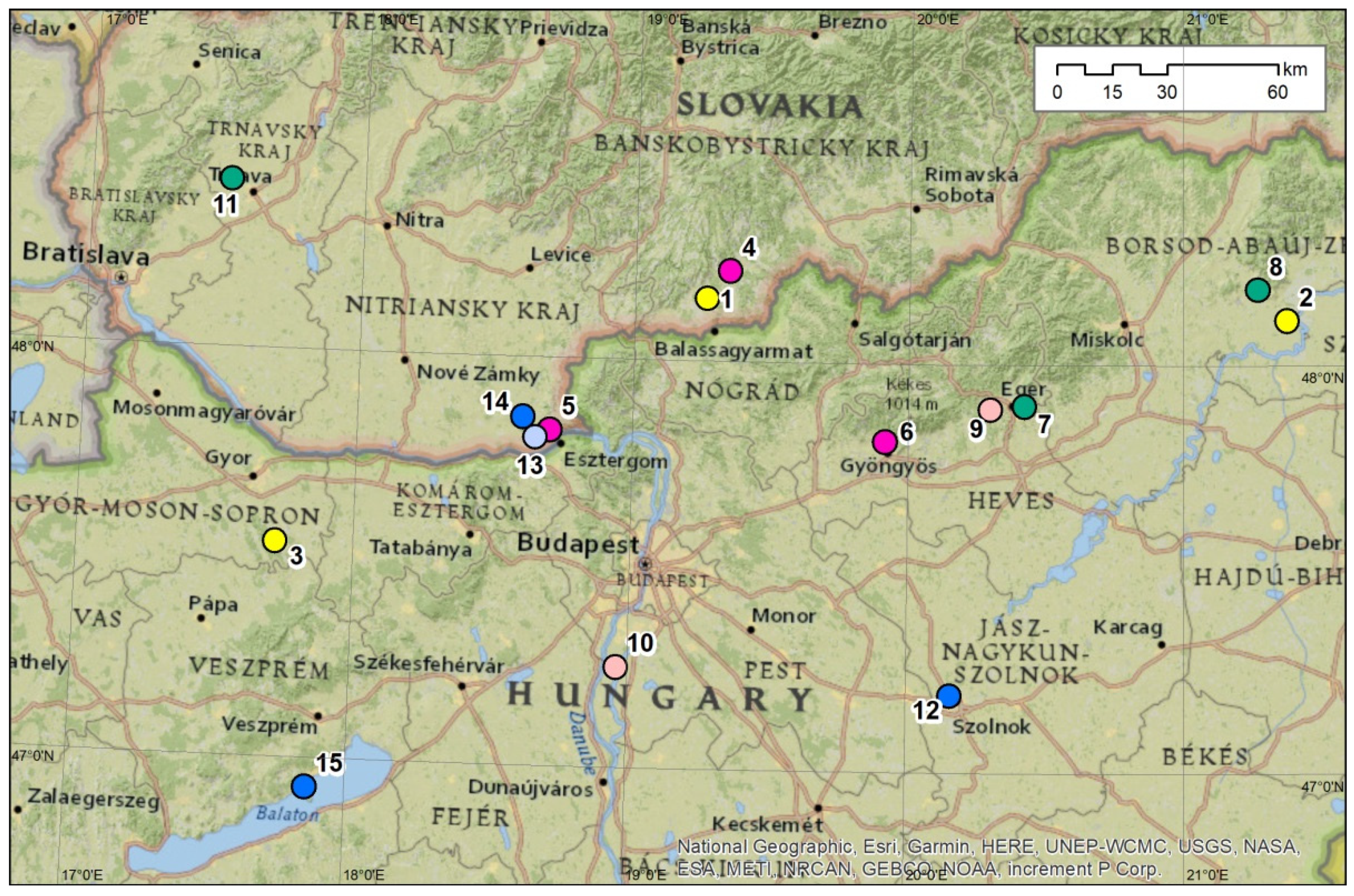
The thesis of this interpretation is as follows: a precisely defined type of morpho-pedotop presents equal micro-climate and a soil ecological condition on whatever sites it occurs in the given territory. Therefore, if we obtain a measured dataset on the micro-climate and soil ecological condition on a site with a detailed defined morpho-pedotop type, the same micro-climatic and soil ecological conditions will occur on all sites with this certain type of morpho-pedotop wherever it occurs in the entire area [28,29,30]. In addition, it is possible to define relative differences in other morpho-pedotops compared to measured ones. For example, these may be warmer or colder or drier or wetter than the measured morpho-pedotops.

The entire process was conducted using GIS techniques. The results provide support for decisions on precise agricultural management [31,32,33].

2.2. Study Area

The project was applied for chosen viticulture areas on the cross-border between Slovakia and Hungary, where advanced sensor stations were installed for permanent monitoring of specific climate data for disease forecasting (SmartVineyard^TM sensor stations, developed by QuantisLabs Ltd., Budapest University of Technology and Economics). The project comprised 3 model areas covering 2522 km² in Slovakia and 12 model regional areas in Hungary. The total area was 9412 km² spread throughout the viticultural regions.

However, this article presents the elaboration of the selected part of this area only. The localisation of these areas is seen in Figure 4.

Herein, we investigated the relative differences in morpho-pedotops’ thermal and moisture conditions on all sensor sites and the entire territory. The detailed defined morpho-pedotops’ conditions enabled spatial interpolation of the measured quantitative data in the whole territory regardless of where measurements were taken.

The characteristics of input indices in Slovakia and Hungary differ to some extent. The Slovak study sites were processed on a topical level to develop interpretation and interpolation for each morpho-pedotop on a detailed 10 × 10 m grid scale. The Hungarian study site scale was 100 × 100 m grid, which responds to the interpretation on a regional level. This difference shows the possibility to apply the described methods of interpretation on a different scale according to the availability of more or less detailed data.

2.3. Data: The Input Indices and Their Analyses

Table 1. List of analysed indices in the study areas. The indices applied to the study areas are marked with an “x”.

The Analysed Index	Applied in Slovakia	Applied in Hungary	Form
Digital Terrain Model	x	x	Raster
Morphometric indices
Slope angle	x	x	Raster
Horizontal and profile (normal) curvature of the relief	x	x	Raster
Orientation of the relief to the cardinal points	x	x	Raster
Contributing area	x	x	Raster
Horizontal and vertical dissection of the relief		x	Raster
Complex forms of the relief		x	Raster
Lengths of the insolation	x	x	Raster
Amount of sun radiation	x	x	Raster
Macroclimatic indices
Average temperature	x		Raster
Beginning and ending days of characteristic temperatures	x		Raster
Days with frost and fog	x		Raster
Cloudiness	x		Raster
Abiocomplex(the values of these analytical characteristics are valid for the areas of abiocomplexes)
Altitude above the sea level of the abiotops	x		Polygon
Morphological types of the relief of the abiotops	x		Polygon
The slope angle of the abiotops	x		Polygon
Normal and horizontal curvature of the abiotops	x		Polygon
Aspect of the abiotops	x		Polygon
Type and texture of the soils	x	x	Polygon
Depth and skeleton of the soils	x	x	Polygon
Moisture and fading point of the soils	x		Polygon
Geological substratum complex	x	x	Polygon
Flow capacity coefficient of the substratum	x		Polygon
Filtration coefficient k of the substratum	x		Polygon
Water storability coefficient	x		Polygon
Depth of the underground water	x		Polygon
Complex interpreted indices
Surface run-off	x		Raster
Erosion threat—potential and real	x		Raster
Potential evapotranspiration—vegetation period	x		Raster
Humidity balance—vegetation period	x		Raster
Topographical humidity index	x		Raster
The balance of the surface water run-off		x	Raster
The humidity balance of the morpho-pedotops		x	Raster

lists the analysed indices for the Slovak and Hungarian study areas. The Slovak topical characteristics are more detailed because of the 10 × 10 m pixel scale and they characterise topical dimension, since Hungarian indices highlight regional differences, and those results present the predominant, average, or prevailing index values on relevant areas (Table 1).

The indices used in the further process have different roles and importance. While we used several referenced methods for particular analyses, the description of these methods is outside the scope of this article. The brief description of selected input indices is therefore as follows:

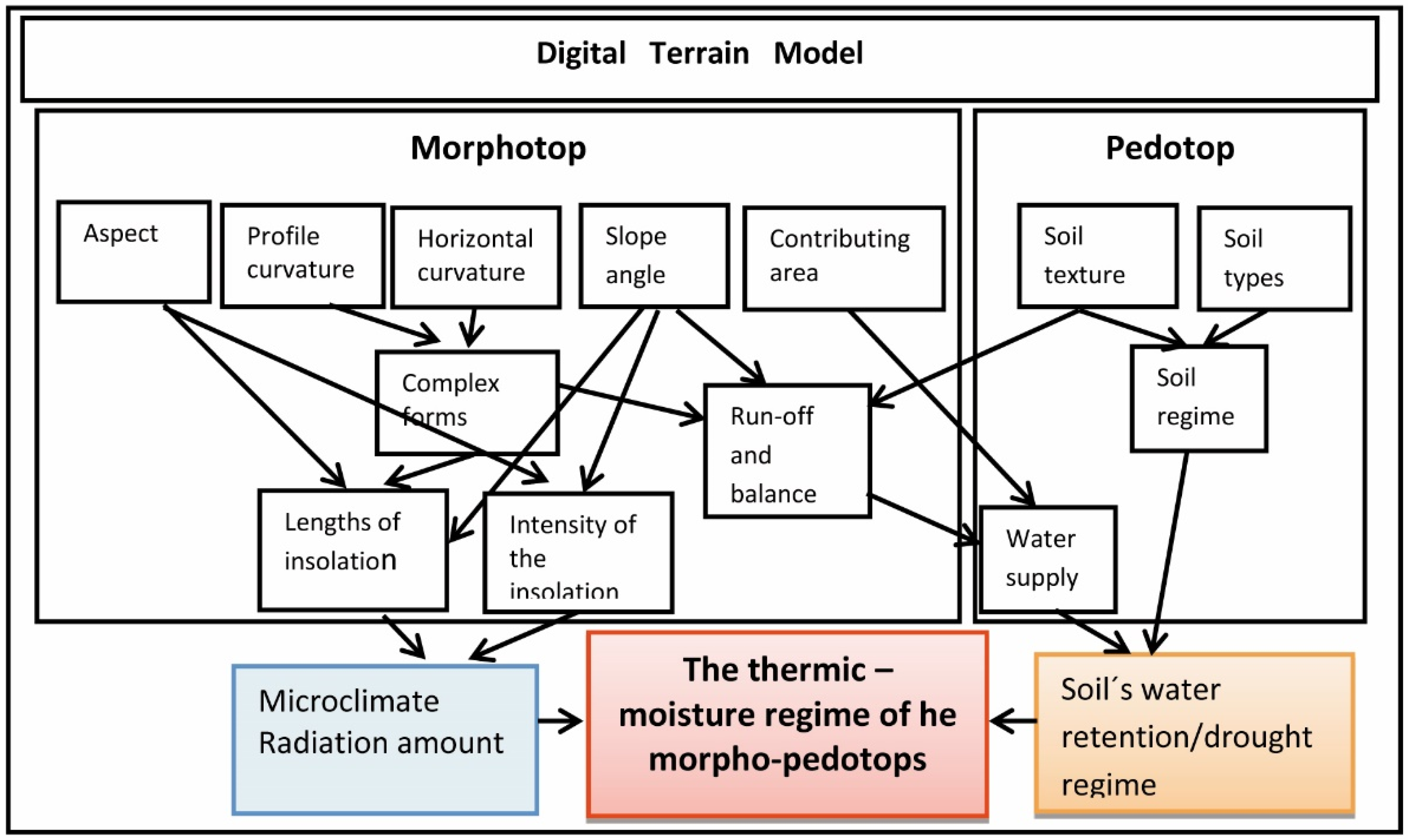
2.3.1. Spatial Frame and Cartographic Base—Digital Terrain Model (DTM)

The original 100 × 100 m raster size was interpolated according to the method of Jarvis et al. [34] to a 10 × 10 m grid for study areas in Slovakia. This cartographic base created on the data on geographic coordinates φ (geographical latitude), λ (geographical longitude), and h (height above sea level) was the framework for all data layers and calculation of all morphometric indices.

2.3.2. Morphometric Indices

Morphometric indices have utmost importance because they form the basis for all re-calculations, re-classifications, and interpretations. They were derived from DTM.

Slope angle is calculated by the “neighbourhood” algorithm [35]. The slope is the decisive index for the amount and velocity of surface run-off and calculation of insolation through the angle of sun rays on the relief.

Horizontal curvature and the profile (normal) curvature of the relief: The attribute of both curvatures is a non-dimensional figure in extension <−1, 1> expressing concave <−1 to 0>, linear <0>, and convex forms <0 to 1>. The horizontal curvature expresses the flexion of the contour lines, and this is the decisive index for the surface run-off direction, which may be concentrated, equilinear, or dispersed. The profile curvature expresses the flexion of the gravity curves, which are rectangular to the contour lines. The index is decisive for balanced, accelerated, or decelerated run-off tendency.

Orientation of the relief towards the cardinal points—the aspect: This expresses the relief orientation grades against <0° to 360°> compass in extension. The index is decisive in insolation calculation.

Contributing area: The m² size of the area from which the run-off flows to the defined spot (pixel). This is calculated by the “result vector” Dinf algorithm [36,37]. The index is decisive in estimating the amount of run-off to the evaluated spot.

Horizontal and vertical dissection of the relief: This is the “classic” index for horizontal and vertical dissection of the relief [38] and it is important in the estimation of the optimum use of the territory.

2.3.3. Morpho-Climatic Indices

Length of insolation: the length of the insolation for the 1 April–31 October vegetation period, and for the hours in each of these months. The model estimates the daily and seasonal changes in sun declination and primary morphometric indices, including slope angle, aspect, and terrain shading by surrounding relief. The index was calculated by a specific module of the spatial analyst application in the GIS ARC Map. This is the basic index for estimating the agricultural units’ thermal regime.

Amount of sun radiation: This expresses the amount of direct and diffuse radiation affecting the relief in Wh·m⁻² for the given period. We calculated this for the vegetation period and each month from April to October. The index was calculated by a specific module of the spatial analyst application in the GIS ARC Map. This is the most important index for estimating microclimate conditions.

2.3.4. Macroclimatic Data and Their Topic Interpretation

This was interpolated from long-term statistical data collected by 76 meteorological stations in Slovakia. It provided average temperature for the vegetation period, beginning and ending days of characteristic temperatures, and temperature extremes such as frost, fog, and cloudiness. They were recalculated by radiation coefficient and the coefficient of relief depression to each abiocomplex at the topic level according to our method.

2.3.5. Abiocomplex: This Consolidates the Index Set of Soil, Relief, and Geology

The list in Table 1 shows that this layer covers the synthetic, homogenous, and consolidated landscape ecological units containing basic indices on abiocomplex indices in polygon form. All attributes were mutually harmonised according to their logical relationships, and the georelief forms the basis for delineating the abiocomplex area borders. Soil properties include the types and the texture (granularity). The source was the portal AGROTOPO GIS, which provided the spatial distribution of the soils http://maps.rissac.hu/agrotopo (accessed on 14 February 2014). Finally, classification elucidated the soil water permeability, which affects the hydro-physical conditions. This index is most important in estimating the soil surface run-off, erosion, and thermal regime.

2.3.6. Complex (Partial Synthetic) Indices

These indices are based on interpretation of the following morphometric, abiocomplex, and climate indices:

Surface run-off: This expresses the average coefficient value of the surface run-off calculated from the abiocomplex and morphometric indices [25].

Erosion threat—potential and actual: This expresses the potential erosion threat, not considering land cover. It is calculated according to the RUSLE model [39]. The actual erosion threat also considers factor C—the land cover influence. The calculated values are classified in t/ha/year in six erosion threat classes [40].

Potential and actual evapotranspiration—vegetation period: These are calculated by the empirical relationship between air temperature and length of insolation.

Humidity balance—vegetation period: This provides the difference between precipitation summation and potential evapotranspiration [41].

Topographical humidity index: This complex index expresses the moisture regime of the soils derived from the contributing area size, slope angle, and hydro-pedologic conditions.

2.4. Syntheses and Interpretations

All the above analytical data were arranged in a consolidated database on a unified cartographic basis by GIS techniques and methods by ESPRIT, Ltd., Banská Štiavnica. This enabled the reading, evaluation and interpretation of all analysed data on each territory unit and provided the set of values of morpho-pedotop properties.

This database gives a broad scope for the interpretation of different tasks. This article presents two decisive direction interpretations of morpho-pedotop properties, namely the microclimate conditions according to the radiation amount and the soil water regime. In complexity, it resulted in the characteristic of the morpho-pedotop thermal–moisture regime.

Unfortunately, reliable measured information on these conditions is available only at the sparse net of meteorological stations and other sensors. Therefore, we developed an interpretation process to compensate for this lack of accurate information. This enabled the definition of the thermal–moisture regime of each territory unit with semi-quantitative characteristics and also the determination of the differences on the sites with sensors and each other unit in the study territory.

Although this process is on a relative scale and is simple, it requires quite complex procedures using logic and diverse methods to achieve the necessary results. It is based on landscape ecological knowledge and methods. Figure 1 outlines the sequential interpretation scheme from initial DTM to the ultimate morpho-pedotops’ thermal–moisture conditions.

Complex interpretation of the input data was required because measurement of this characteristic on the entire area is impossible. This process required the following summarised steps:

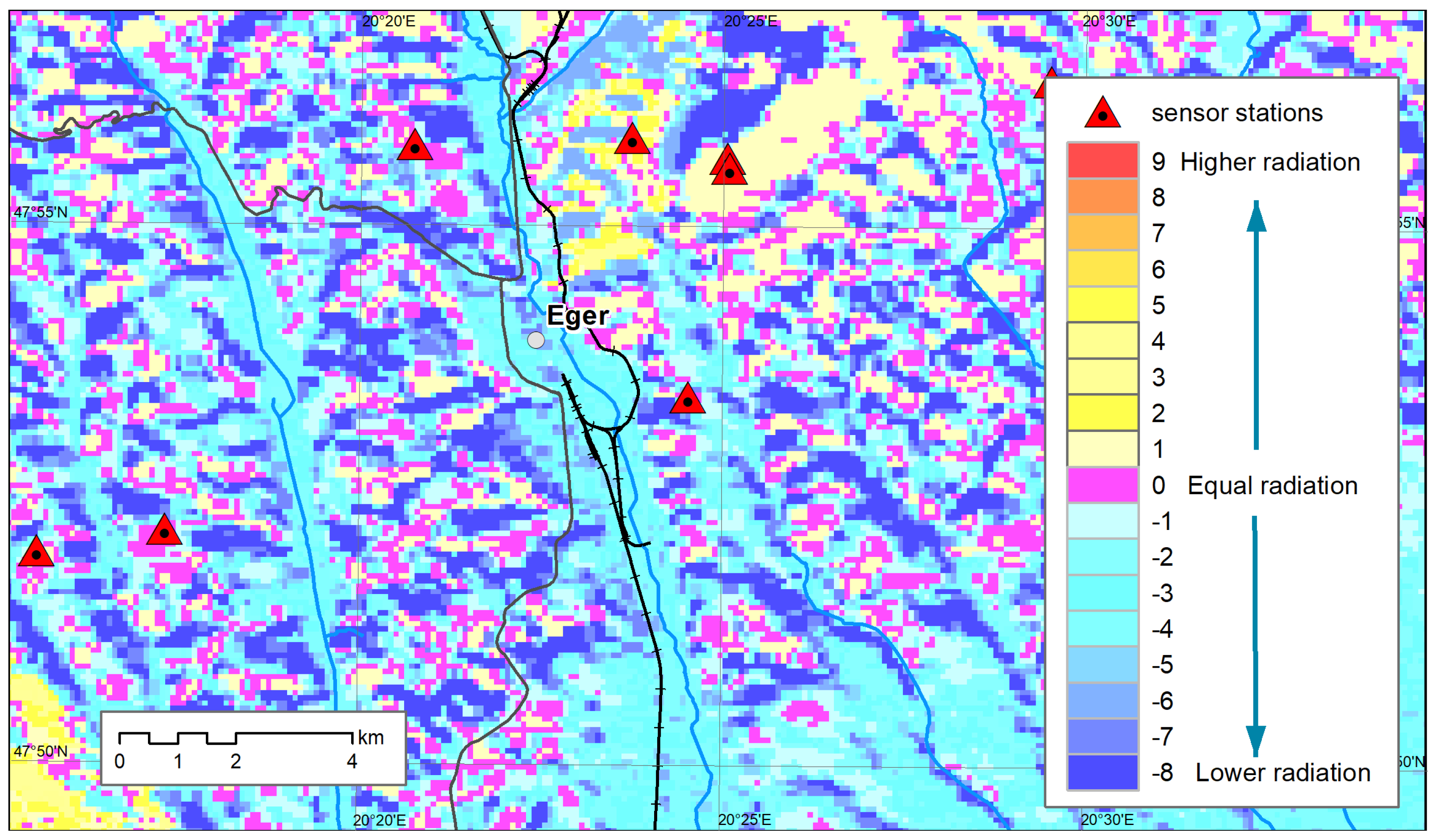
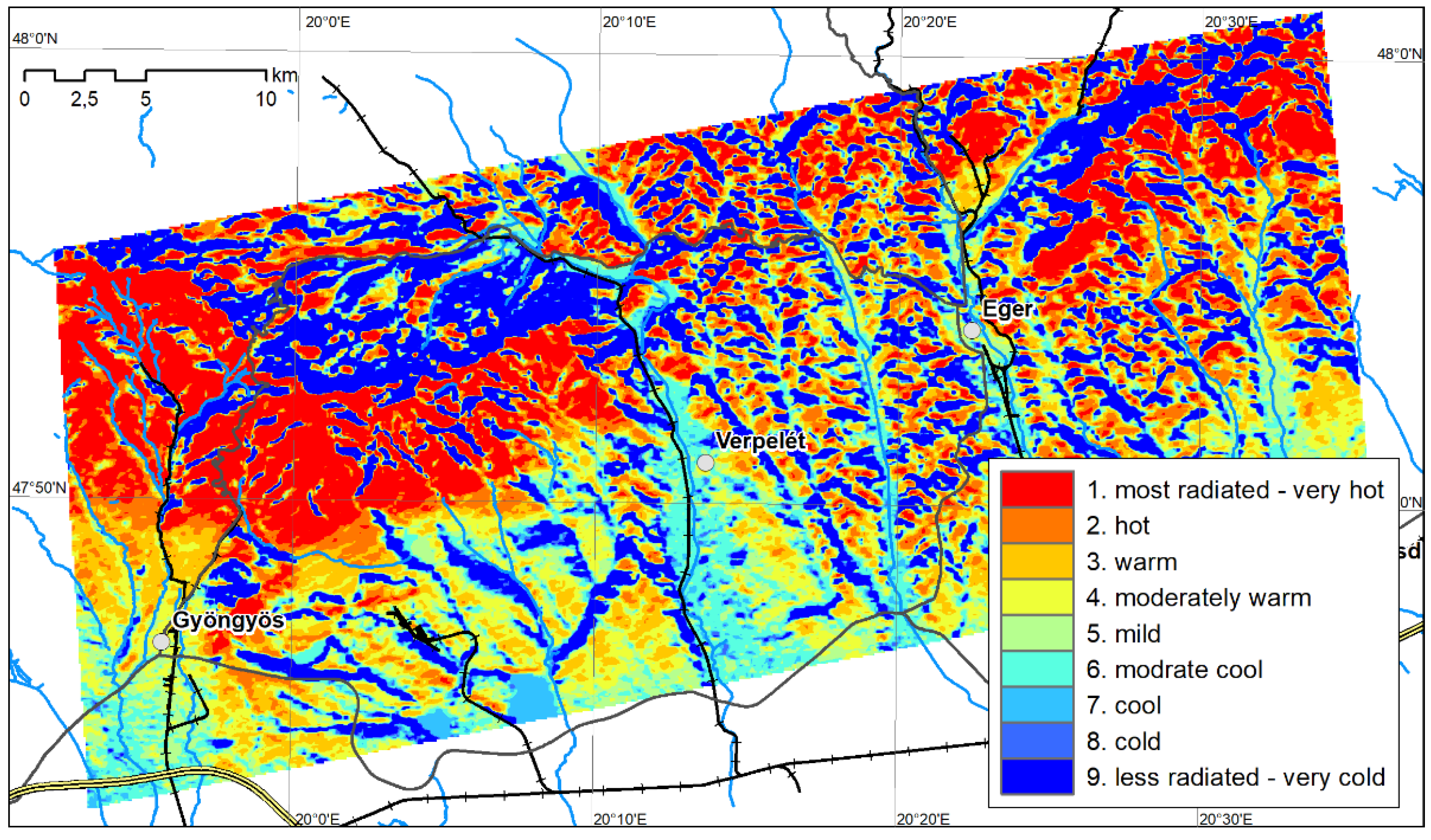
• Interpretation of micro-climate differences: The astronomic data, such as the sun trajectory on the orbit and its seasonal changes, are stable for the given climate and geographical region, and the differences in the microclimate are expressed basically by the diversity of the morphometric indices of the georelief—namely by slope angle, aspect, and shading. The differences were interpreted according to the amount of solar radiation on the relief surface [42,43]. The length timing and amount of direct sun radiation are summarised for each month, and for the entire 1 April to 31 October vegetation period.
• Definition of the tendency and direction of water and material movement on the base of the horizontal and profile curvature of relief forms. The horizontally concave curvature of the relief determines the concentrated, the uncurved relief the linear, and the convex relief the dispersed direction of the run-off. The profile concave curvature determines decelerated run-off, the non-curved portion equable run-off, and convex curvature indicates accelerated run-off.
• Definition of the balance of the water and material movement based on the topographic position and complex forms of relief. This determines movements from accelerated dispersed removal up to decelerated concentrated accumulation.
• Calculation of the amount of water arriving at the unit from surface or underground.
• Flow based on the size of the area above the evaluated unit; this is defined as the contributing area.
• Determination of the morpho-pedotop run-off index. This provides the rate of infiltrated and outflow water based on soil and slope architecture [44].
• Estimation of the aggregate morpho-pedotop water supply from the combination of the balance of the water movement and the size of the contributing area in the relative classes. These classes provide the input values for the interpretation of the moisture regime and the morphotop topographic humidity. This is illustrated by the vertical axis in

  Table 2. Relative values of the moisture regime and morpho-pedotop topographic humidity. (Moisture regime of the soils: 1—very dry and coarse morpho-pedotops, 2—dry, sandy morpho-pedotops, 3—balanced morpho-pedotops, 4—moist morpho-pedotops, 5—wet morpho-pedotops, 6—very wet, water-logged morpho-pedotops).

  Soil Types—MoiSture and Retention Surface Water Supply	1—Coarse Scelet, Sands, Salty	2—Sandy	3—Loamy–Sandy to Sandy–Loamy	4—Loamy to Silty–Loamy	5—Clay–Loamy to Silty–Loamy	6—Silty–Clay to Clay	7—Alluvial,Gley, Salty–Gley	8—Organic, Peat
  1—only outflow, dispersion, and removal	1	1	1	2	2	2	5	6
  2—weak prevailing outflow and removal	1	1	2	2	3	3	5	6
  3—balanced inflow and outflow	1	2	2	3	3	4	5	6
  4—moist prevailing inflow and accumulation	1	2	3	3	4	4	5	6
  5—wet massive inflow, accumulation	2	3	3	4	4	5	5	6
  6—extremely wet, only inflow	3	5	5	6	6	6	6	6

  .
• Determination of soil retention potential based on the soil type and texture defined in the following 1 to 8 graded scale, from 1—skeleton soils, sands, and other coarse materials that cause rapid soil infiltration and thus also quick drying out in extremely dry soils; up to: 7—wet, water-logged, gley, and sometimes salinated soils permanently influenced by underground water as extremely wet soils; 8—peat. The normal, and not extreme, soil types are ranked according to their texture from 2 to 6 on the horizontal axis in Table 2.
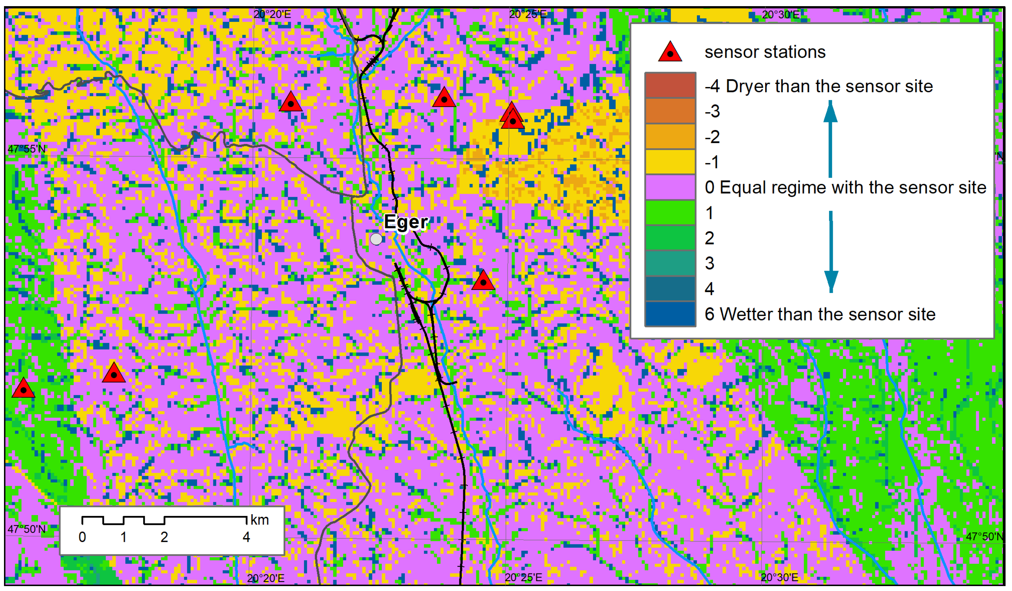
• Final determination of the moisture regime of the morpho-pedotops based on the combination of soil types and water supply in the relative 6-grade scale (Table 2).

Note: The more detailed analyses on 10 × 10 m grid size in the Slovak study areas enabled greater complexity in deriving the soil moisture regime. Additional indices include the filtration coefficient, field moisture, fading point, the coefficients of substratum flow capacity and water storage, underground water depth, and the potential and actual evapotranspiration, as depicted in Table 1. Nevertheless, the basic approach and formation of results were identical to those described for the Slovak and Hungary study areas.

3. Results

The figures highlight cuts from the Mátra and Bükk mountains study area in Northern Hungary. The same process was applied for each study area.

3.1. Microclimatic Conditions

The resultant value is the amount of radiation approaching the surface of the relief, as the basic morpho-climatic characteristic [42,43]. The length and amount of direct solar radiation are presented for the vegetation period, i.e., 1 April to 31 October.

The sun radiation calculation for this territory varied from 810.378 Wh·m⁻² to 995.009 Wh·m⁻² during the vegetation period. These values were ranked in nine classes, from 1 for the most radiated and hot morphotops to 9 for the least radiated and very cold morphotops. The classes are in 20.514 Wh·m⁻² incremental steps in the vegetation period. These classes were used for further interpretation in tables and maps (Figure 2). Finally, the amount of radiation defines the relative differences in thermal and moisture conditions in each terrain unit’s climate area because the macro-climate conditions in the study areas are almost homogenous. This knowledge is most important in applying agricultural procedures, and it is decisive for chemical application and the prediction of plant disease.

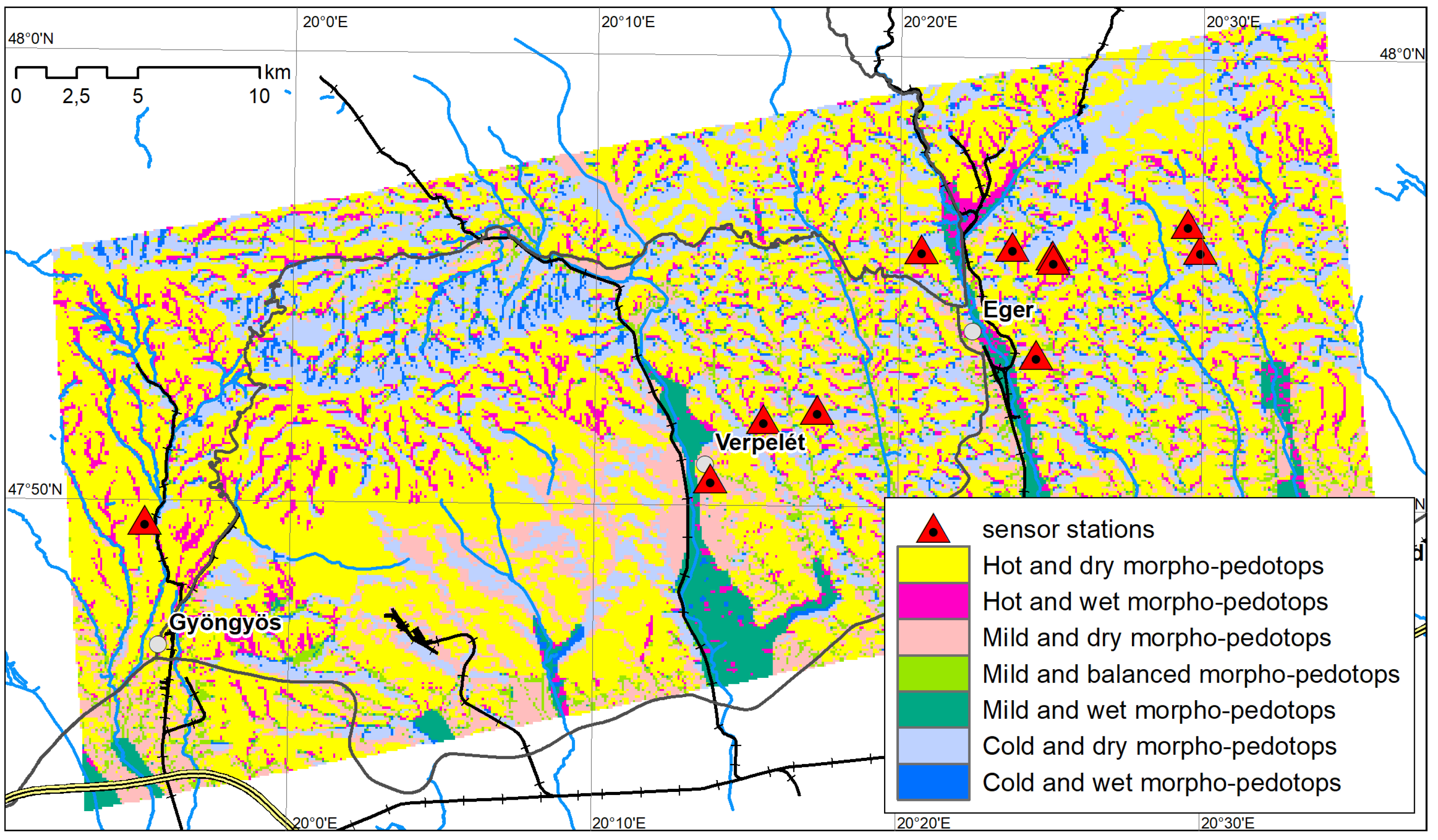
3.2. Pedologic Conditions

In addition to dependence on micro-climate conditions, the site’s complex thermal–moisture regime is influenced by the soil’s ability to maintain and release heat and water.

The moisture regime was defined by topographic information on the relief and soils, which determine site humidity. This index, therefore, has its correct designation as morpho-pedotop´ topographic humidity.

The result is constituent of the complex morpho-pedotops moisture regime as presented in Table 2 and Figure 3.

3.3. Complex Interpretations: The Morpho-Pedotops’ Thermal–Moisture Regime

The complex interpretation resulted in the final integrated definition of relief radiation and soil moisture regime as the morpho-pedotops’ thermal–moisture regime (

Table 3. Integrated characteristics of the morpho-pedotop thermal–moisture regime.

Moisture Regime (Table 2, Figure 3) Thermal Regime (Radiation, Figure 2)	1. Very Dry	2. Dry	3. Balanced	4. Moist	5. Wet	6. Very Wet
1. very hot	1.1 very dry/ very hot	1.2	1.3	1.4	1.5	1.6 very wet/ very hot
2. hot	2.1	2.2	2.3	2.4	2.5	2.6
3. warm	3.1	3.2	3.3	3.4	3.5	3.6
4. moderately warm	4.1	4.2	4.3	4.4	4.5	4.6
5. mild	5.1	5.2	5.3	5.4	5.5	5.6
6. moderate cool	6.1	6.2	6.3	6.4	6.5	6.6
7. cool	7.1	7.2	7.3	7.4	7.5	7.6
8. cold	8.1	8.2	8.3	8.4	8.5	8.6
9. very cold	9.1 very dry/ very cold	9.2	9.3	9.4	9.5	9.6 very wet/ very cold
Generalised groups of the thermal–moisture regime by words and colours.

). The results present the relative differences in morpho-pedotop indices. The morpho-pedotops’ thermal–moisture regime was defined for each study area unit.

Each square on the table reflects their combination based on the absolute radiation and soil property values. The cornerstone values rank from very dry and very hot morpho-pedotops to mild types and then through to very wet and very cold species. The different colours highlight the general characteristics of the radiation–moisture regime.

Table 4. Selected characteristics of the sensor localities (the colour distinction is the same as in Table 3).

No.	The Locality of the Sensors (Region/Community)	Radiation/Moisture Combinations Table 3	Radiation Wh·m−2	Radiation Classes Figure 2	Moisture Regime of the Soils Table 2	Altitude m.a.s.l.
1.	Nenince	1.1	925880	1	1	206
2.	Tokaj DK	1.3	954894	1	3	173
3.	Győr, Écs	2.2	914129	2	2	206
4.	Velky Krtís, Naturalvino	2.4	910636	2	4	254
5.	Štúrovo, Obid	3.4	904202	3	4	159
6.	Mátra Gyongyossolymos	3.5	907508	3	5	267
7.	Bukk Eger É	4.2	889383	4	2	266
8.	Tokaj DNy Tarcal	4.4	891092	4	4	101
9.	Mátra Bukk Verpelét	5.1	880759	5	1	143
10.	Szigetsz.márton	6.2	878054	6	2	97
11.	Zvoncin	6.3	877734	6	3	158
12.	Szolnok	7.6	876720	7	6	83
13.	Štúrovo Mužla J	8.3	869392	8	3	120
14.	Štúrovo Mužla S	8.5	869240	8	5	120
15.	Balaton É Tihany	9.3	831734	9	5	136

lists the most important morpho-pedotop characteristics at selected sensor station localities with their different characteristic combinations. Figure 4 shows the location of selected sensors. Identical characteristics were produced in all 49 sensor sites and the entire studied area. The result presents the relative differences in the objectively defined and mapped thermal–moisture conditions on each spot of sensor stations (Figure 2 and Figure 3).

This is the basic result for all interpretations and the comparison of conditions on sensor sites and all the other units in the territory. It also provides the basis for reliable interpolation of the measured values on both sensor station sites and non-sensor territory units.

The next steps were based on specifications of the relationships between morpho-pedotops on the sensor station sites and those on the remaining study area. The logical process we followed is contained in the following comparison and interpolation section.

3.4. Comparisons and Interpolation

The comparison of the characteristics of the individual pedotops’ qualitative differences enables us to provide a reliable interpolation of the measured microclimate values permanently measured by sensors, since:

• These measured values determine phenologic phases and thus forecast disease formation and escalation, and they can suggest protective management decisions.
• This is a reasonable prediction that the time course of the phenologic and disease phases should be the same, or very similar, on each morpho-pedotop with the same exactly defined conditions as those on sensor sites.
• We can qualitatively and quantitatively define if a given morpho-pedotop on sites without sensors is colder or warmer and wetter or dryer than those on monitored sensor station sites (Figure 5, Figure 6 and Figure 7).
• Thus, we can reasonably suggest that the time course for management actions should also be the same, or very similar, on each morpho-pedotop with the same exactly defined conditions as those on sensor sites, which are usually based on the measured microclimate date.

4. Discussion

Sustainable precise agriculture requires a decision support system based on site-specific information. This information can be based on different approaches, including combined traditional analytic techniques and advanced measurements, as well as interpretation models [45,46,47,48]. Nevertheless, generally speaking, the agricultural practice depends prevailingly on the measured analytical data, which serve for normative decisions on management actions.

Although device-measured data are most often used, the measured values are also results of the synergy of all invariable conditions that were defined or the morpho-pedotops. Thus, also the data achieved not by measuring but by the interpretation procedure of the same data can provide the basis for spatially precise and site-specific action in field management and plant protection, for the forecast of earlier or later disease development and for the location of temperature/moisture-sensitive cultures [4]. Nevertheless, the methods for this type of interpretation are quite rare.

The above-presented process of the purpose-oriented interpretations mirrors the balance of water, solutes, and heat—the thermal–moisture regime in morpho-pedotops. Nevertheless, the process and results can be used—regardless of above-mentioned results—for the interpretation of the erosion and/or accumulation models, water retention and accumulation, the transport of chemicals, flooding danger, the overall protection of the ecological stability of the landscape, and other management procedures [15,49,50,51].

It is important to state that the presented interpolation method differs from the “classic” mathematic–geometric interpolation of the meteorological data monitored by meteorological stations. The classic interpolation usually results in defined isolines, including those for temperature and humidity. These isolines do not usually reflect detailed relief, soil, and micro-climatic conditions. On the other hand, our presented interpolation of the thermal–moisture regime markedly relies on the exact relief and soil characteristics. Moreover, our approach combines whole-area morpho-pedotop mapping with information collected by traditional measuring. This is an appropriate method for defining decisive conditions for site-specific agriculture. It provides a better basis for the precise spatial projection of preconditions required for management actions than the mathematical interpolation of data obtained from remote meteorological stations.

The sensors in our study areas were specifically established to provide continual microclimate data for an advanced forecast programme on the development of grape disease and proposed consecutive and timely precise use of protective chemicals. However, it is most important to mention that both the forecast models and analyses of measured data are outside the scope of this article.

5. Conclusions

According to the objectives, the study results are divided into the following basic groups:

• The analyses of the morphologic and pedologic conditions and their mapping on the whole study area. Their syntheses resulted in the definition of morpho-pedotops. These results have basic research character;
• The purpose-oriented morpho-pedotop interpretation projects the study area’s complex thermal and moisture conditions. Our results here have applied research character;
• The interpolation, comparison, and definition of the relative differences in objective thermal–moisture regime characteristics site-specific for the entire territory. This provides the basis for sustainable field management, which can transform research results into appropriate agricultural practice. This part of our result has practical character.

Concerning the validity of the result, it is important to note that the input data on relief and soils are exact and objective, as well as their synthesis to morpho-pedotops. The interpretation of their thermal–moisture regime is a logical process, based on calculations and other knowledge. Therefore, the results—the defined interpolation, comparisons, and definitions of the relative differences—should also be correct.

Although this process could be permanently improved, the results are already suitable for both plant protection and—if combined with measured data—also for disease prediction. Besides this, our results can also be used as important information for the integrated land resource management defined in Agenda 21 Chapter 10 [1,52,53] (pp. 516–521). Researchers further report that site-specific land management will influence all of the following: crop production [54,55], lower chemical use and protection against soil erosion, extreme run-off, and flooding [15], and the loss of biodiversity and overall landscape ecological stability [56] (pp. 395–423).

The spatial interpretation of measured data according to the spatial distribution of exactly defined morpho-pedotops is reasonable and logical. Therefore, the further development of this interpretation should lean on the precision of input data—this means the precision of the digital model of the relief on a more detailed raster or applying a vector approach, and more detailed data on the spatial distribution of the soil properties. Additionally, the interpretation of microclimate data might also be permanently improved. Finally, our results are intended to inspire scientific programmes that refine the interpretation, interpolation, and modelling of existing conditions and future forecasts.

References

1. Schieffer, J.; Dillon, C. The economic and environmental impacts of precision agriculture and interactions with agro-environmental policy. Precis. Agric. 2015, 16, 46–61. [Google Scholar] [CrossRef]
2. Mcbratney, A.; Whelan, B.; Ancev, T. Future Directions of Precision Agriculture. Precis. Agric. 2005, 6, 7–23. [Google Scholar] [CrossRef]
3. Qin, C.Z.; Zhu, A.X.; Pei, T.; Li, B.L.; Scholten, T.; Behrens, T.; Zhou, C.H. An approach to computing topographic wetness index based on maximum downslope gradient. Precis. Agric. 2011, 12, 32–43. [Google Scholar] [CrossRef]
4. Kerényi, A.; Csorba, P. Assessment of the sensitivity of the landscape in a sample area in Hungary for climatic variability. Earth Surf. Process. Landf. 1991, 16, 663–673. [Google Scholar] [CrossRef]
5. Hreško, J.; Boltižiar, M. The influence of the morphodynamic processes to landscape structure in the high mountains (Tatra Mts.). Ecology 2001, 20, 141–149. [Google Scholar]
6. Wrbka, T.; Erb, K.H.; Schulz, N.B.; Peterseil, J.; Hahn, C.O.; Haberl, H. Linking pattern and process in cultural landscapes. An empirical study based on spatially explicit indicators. Land Use Policy 2004, 21, 289–306. [Google Scholar] [CrossRef]
7. Jongman, R.H. Homogenisation and fragmentation of the European landscape: Ecological consequences and solutions. Landsc. Urban Plan. 2002, 58, 211–221. [Google Scholar] [CrossRef]
8. Antrop, M. Background concepts for integrated landscape analysis. Agric. Ecosyst. Environ. 2000, 77, 17–28. [Google Scholar] [CrossRef]
9. Bastian, O.; Krönert, R.; Lipský, Z. Landscape Diagnosis on Different Space and Time Scales—A Challenge for Landscape Planning. Landsc. Ecol. 2006, 21, 359–374. [Google Scholar] [CrossRef]
10. Mizgajski, A.; Markuszewska, I. (Eds.) Implementation of landscape ecological knowledge in practice. In The Problems of Landscape Ecology; Polish Association for Landscape Ecology, Wydawnictvo Naukowe Adam Miczkiewicz University: Poznań, Poland, 2010; Volume 28, p. 271. [Google Scholar]
11. AGENDA 2l. Integrated Approach to the management of Land resources. In Proceedings of the United Nations Conference on Environment and Development, Rio de Janeiro, Brazil, 3–14 June 1992. Chapter 10. [Google Scholar]
12. Izakovičová, Z.; Miklós, L.; Miklósová, V. Integrative assessment of land use conflicts. Sustainability 2018, 10, 3270. [Google Scholar] [CrossRef] [Green Version]
13. Pacheco, F.A.L. Sustainable Use of Soils and Water: The Role of Environmental Land Use Conflicts. Sustainability 2020, 12, 1163. [Google Scholar] [CrossRef] [Green Version]
14. Reed, J.; Van Vianen, J.; Barlow, J.; Sunderland, T. Have integrated landscape approaches reconciled societal and environmental issues in the tropics? Land Use Policy 2017, 63, 481–492. [Google Scholar] [CrossRef]
15. Band, L.; Tagu, C.; Brun, S.; Tenenbaum, D.; Fernandez, R. Modelling watersheds as spatial object hierarchies: Structure and dynamics. Trans. GIS 2000, 4, 181–196. [Google Scholar] [CrossRef]
16. Belčáková, I. New approaches to the integration of ecological-social and economic aspects in land use planning. Ekológia 2003, 22, 183–189. [Google Scholar]
17. Behrens, T.; Scholten, T. Digital Soil mapping in Germany—A review. J. Plant. Nutr. Soil Sci. 2006, 169, 434–443. [Google Scholar] [CrossRef]
18. Schmidt, K.; Behrens, T.; Friedrich, K.; Scholten, T. A method to generate soilscapes from soil maps. J. Plant. Nutr. Soil Sci. 2010, 173, 163–172. [Google Scholar] [CrossRef]
19. Howard, J.A.; Mitchell, C.W. Phytogeomorphology; Wiley: New York, NY, USA, 1985. [Google Scholar]
20. Miklós, L. Morphometric indices of the relief in the LANDEP methods and their interpretation. Ecology (Czechoslovak Federative Republic) 1991, 10, 159–186. [Google Scholar]
21. Pauditšová, E.; Slabeciusová, B. Modelling as a platform for landscape planning. In Proceedings of the 14th International Multidisciplinary Scientific GeoConferences SGEM 2014, Albena, Bulgaria, 17–26 June 2014; Volume 3, pp. 753–760. [Google Scholar]
22. Falťan, V.; Pírová, L.; Petrovič, F. Detailed mapping of geocomplexes in the vineyard landscape. Folia Oecologica 2016, 43, 138–146. [Google Scholar]
23. Krcho, J. Georelief as a subsystem of landscape and the influence of morphometric parameters of georelief on spatial differentiation of landscape-ecological processes. Ecology 1991, 10, 115–158. [Google Scholar]
24. Miklós, L.; Kočická, E.; Izakovičová, Z.; Kočický, D.; Špinerová, A.; Diviaková, A.; Miklósová, V. Landscape as a Geosystem; Springer: Cham, Switzerland, 2019; p. 161. [Google Scholar] [CrossRef]
25. Brath, A.; Montanari, A. The effects of the spatial variability of soil infiltration capacity in distributed rainfall-runoff modelling. Hydrol. Process. 2000, 14, 2779–2794. [Google Scholar] [CrossRef]
26. Csorba, P. Landscape ecological fragmentation of the small landscape units (Microregions) of Hungary based on the settlement network and traffic infrastructure. Ecology 2008, 27, 99–116. [Google Scholar]
27. Súľovský, M.; Falťan, V.; Skokanová, H.; Havlíček, M.; Petrovič, F. Spatial analysis of long-term land-use development regarding physiotopes: Case studies from the Carpathians. Phys. Geogr. 2017, 38, 470–488. [Google Scholar] [CrossRef]
28. Łowicki, D.; Mizgajski, A. Typology of physical-geographical regions in Poland in line with land-cover structure and its changes in the years 1990–2006. Geogr. Pol. 2013, 86, 255–266. [Google Scholar] [CrossRef]
29. Bastian, O.; Grunewald, K.; Khoroshev, A.V. The significance of geosystem and landscape concepts for the assessment of ecosystem services: Exemplified in a case study in Russia. Landsc. Ecol. 2015, 30, 1145–1164. [Google Scholar] [CrossRef]
30. Reina, G. A multi-sensor robotic platform for ground mapping and estimation beyond the visible spectrum. Precis. Agric. 2019, 20, 423–444. [Google Scholar] [CrossRef]
31. Hreško, J.; Mederly, P.; Petrovič, F. Landscape ecological research with the support of GIS tools in the preparation of landscape-ecological plan (model area of the Považská Bystrica city). Ecology 2013, 22, 195–212. [Google Scholar]
32. Field, D.; Morgan, C.L.S.; Mcbratney, A.B. (Eds.) Global Soil Security (Progress in Soil Science), 1st ed.; Springer: Cham, Switzerland, 2017. [Google Scholar] [CrossRef]
33. Morgan, C.L.S.; Yimam, Y.T.; Barlage, M.; Gochis, D.; Dornblaser, B. Valuing of Soil Capability in Land Surface Modelling. In Global Soil Security; Springer: Cham, Switzerland, 2017. [Google Scholar] [CrossRef]
34. Jarvis, A.; Reuter, H.; Nelson, A.; Guevara, E. Hole-Filled SRTM for the Globe: Version 4: Data Grid. CGIAR Consortium for Spatial Information. 2008. Available online: http://srtm.csi.cgiar.org/ (accessed on 4 November 2013).
35. Burrough, P.A.; Mcdonnel, R.A. Principles of Geographical Information Systems; Oxford University Press: Oxford, UK, 1998. [Google Scholar]
36. Tarboton, D.G. A new method for the determination of flow directions and upslope areas in grid digital elevation models. Water Resour. Res. 1997, 33, 309–319. [Google Scholar] [CrossRef] [Green Version]
37. Costa-Cabral, M.C.; Burges, S.J. Digital Elevation Model Networks (Demon): A Model of Flow Over Hillslopes for Computation of Contributing and Dispersal Areas. Water Resour. Res. 1994, 30, 1681–1692. [Google Scholar] [CrossRef]
38. Mazúr, E. (Ed.) Atlas of the Slovak Socialist Republic; SAV, SÚGK: Bratislava, Slovakia, 1980. [Google Scholar]
39. Malíšek, F. Optimisation of the slope lengths in relation to the water erosion. Bratislava. Ved. Práce VÚPÚ 1992, 17, 201–220. [Google Scholar]
40. Šúri, M. The Mapping and Modelling of the Water Erosion with the Remote Sensing Data in GIS; Geografický Ústav Slovenskej Akadémie Vied [Geographical Institute of the Slovak Academy of Sciences]: Bratislava, Slovakia, 1990. [Google Scholar]
41. Blaney, H.F.; Cridle, W.D. Determining Water Requirements in Irrigated Areas from Climatological and Irrigation Data; Soil Conservation Service: Washington, DC, USA, 1950; p. 48. [Google Scholar]
42. Fu, P.; Rich, P.M. The Solar Analyst 1.0 Manual. US Helios Environmental Modelling Institute (HEMI). 2000. Available online: http://citeseerx.ist.psu.edu/viewdoc/download (accessed on 14 February 2014).
43. Fu, P.; Rich, P.M. A Geometric Solar Radiation Model with Applications in Agriculture and Forestry. Comput. Electron. Agric. 2002, 37, 25–35. [Google Scholar] [CrossRef]
44. Kim, H.S. Soil Erosion Modelling Using RUSLE and GIS; Colorado State University: Fort Collins, CO, USA, 2006. [Google Scholar]
45. Whelan, B.M.; Mcbratney, A.B. Definition and Interpretation of potential management zones in Australia. In Proceedings of the 11th Australian Agronomy Conference, Geelong, Victoria, Australia, 2–6 February 2003. [Google Scholar]
46. Mizgajski, A.; Stępniewska, M. Ecosystem services assessment for Poland—Challenges and possible solutions. Ekonomia i Środowisko 2012, 2, 54–73. [Google Scholar]
47. La Rosa, D.; Priviteram, R. Characterization of non-urbanized areas for land-use planning of agricultural and green infrastructure in urban contexts. Landsc. Urban. Plan. 2013, 109, 94–106. [Google Scholar] [CrossRef]
48. Štefunková, D.; Hanušin, J. Viticultural landscapes: Localised transformations over the past 150 years through an analysis of three case studies in Slovakia Institute of Landscape Ecology of the Slovak Ac. Morav. Geogr. Rep. 2019, 27, 155–168. [Google Scholar]
49. Belmans, C.; Wesseling, J.G.; Feddes, R.A. Simulation model of the water balance of a cropped soil: SWATRE. J. Hydrol. 1983, 63, 271–286. [Google Scholar] [CrossRef]
50. De Roo, A.; Thielen, J.; Gouweleuuw, B.; Lisflood, A. Distributed Water-Balance, Flood Simulation and Flood Inundation Model; User Manual Version 1.0; Report of the European Commission; Joint Research Centre: Ispra, Italy, Special Publications No. I.02.131; 2002. [Google Scholar]
51. La Rosa, D.; Barbarossa, L.; Privitera, R.; Martinico, F. Agriculture and the city: A method for sustainable planning of new forms of agriculture in urban contexts. Land Use Policy 2014, 41, 290–303. [Google Scholar] [CrossRef]
52. Jongman, R.H. (Ed.) The New Dimensions of the European Landscapes; Springer Science & Business Media: Dordrecht, Holland, 2004; p. 258. [Google Scholar]
53. Breuste, J.; Haase, D. Workshop 2: Challenges for urban landscape in Europe. In European Landscapes in Transformation: Challenges for Landscape Ecology and Management, Proceedings of the European IALE Conference, Salzburg, Austria, 12–46 July 2009; Breuste, J., Kozová, M., Finka, M., Eds.; Salzburg: Bratislava, Slovakia, 2009; pp. 516–521. ISBN 978-80-227-3100-3. [Google Scholar]
54. Kaspar, T.C.; Colvin, T.S.; Jaynes, B.; Karlen, D.L.; James, D.E.; Meek, D.W. Relationship between six years of corn yields and terrain attributes. Precis. Agric. 2003, 4, 87–101. [Google Scholar] [CrossRef]
55. Slámová, M.; Belčáková, I. The role of small farm activities for the sustainable management of agricultural landscapes: Case studies from Europe. Sustainability 2019, 11, 5966. [Google Scholar] [CrossRef] [Green Version]
56. Izakovičová, Z.; Miklós, L.; Špulerová, J. Basic principles of sustainable land use management. In Current Trends in Landscape Research: Innovations in Landscape Research; Springer Nature: Cham, Switzerland, 2019; pp. 395–423. [Google Scholar]
Figure 1. Sequential interpretation scheme.
Land 10 00940 g001
Figure 2. Amount of solar radiation on morpho-pedotops.
Land 10 00940 g002
Figure 3. Morpho-pedotop moisture regime.
Land 10 00940 g003
Figure 4. Localisation of selected sensors from Table 4; the colour distinction of the dots identifying sensor location is the same as in Table 3.
Land 10 00940 g004
Figure 5. Differences in the amount of solar radiation on morpho-pedotops and sensor station sites (cut).
Land 10 00940 g005
Figure 6. Differences in the morpho-pedotop moisture regime and moisture at sensor station sites (cut).
Land 10 00940 g006
Figure 7. Different combinations of morpho-pedotop thermal and moisture regimes.
Land 10 00940 g007