Article

Are Land Use Options in Viticulture and Oliviculture in Agreement with Bioclimatic Shifts in Portugal?

by
Cristina Andrade
1,2,*,
André Fonseca
2,3 and
João Andrade Santos
2,3,4
1
Natural Hazards Research Center (NHRC.ipt), Instituto Politécnico de Tomar, 2300-313 Tomar, Portugal
2
Centre for the Research and Technology of Agro-Environmental and Biological Sciences (CITAB), Universidade de Trás-os-Montes e Alto Douro (UTAD), 5001-801 Vila Real, Portugal
3
Institute for Innovation, Capacity Building and Sustainability of Agri-Food Production, Universidade de Trás-os-Montes e Alto Douro (UTAD), 5001-801 Vila Real, Portugal
4
Department of Physics, School of Sciences and Technology, Universidade de Trás-os-Montes e Alto Douro (UTAD), 5001-801 Vila Real, Portugal
*
Author to whom correspondence should be addressed.
Land 2021, 10(8), 869; https://doi.org/10.3390/land10080869
Submission received: 20 July 2021 / Revised: 16 August 2021 / Accepted: 17 August 2021 / Published: 19 August 2021
(This article belongs to the Topic Climate Change and Environmental Sustainability)

Abstract

:
Land and climate are strongly connected through multiple interface processes and climate change may lead to significant changes in land use. In this study, high-resolution observational gridded datasets are used to assess modifications in the Köppen–Geiger and Worldwide Bioclimatic (WBCS) Classification Systems, from 1950–1979 to 1990–2019 in Portugal. A compound bioclimatic-shift exposure index (BSEI) is also defined to identify the most exposed regions to recent climatic changes. The temporal evolution of land cover with vineyards and olive groves between 1990 and 2018, as well as correlations with areas with bioclimatic shifts, are analyzed. Results show an increase of CSa Warm Mediterranean climate with hot summer of 18.1%, followed by a decrease in CSb (warm summer) climate of −17.8%. The WBCS Temperate areas also reveal a decrease of −5.11%. Arid and semi-arid ombrotypes areas increased, conversely humid to sub-humid ombrotypes decreased. Thermotypic horizons depict a shift towards warmer classes. BSEI highlights the most significant shifts in northwestern Portugal. Vineyards have been displaced towards regions that are either the coolest/humid, in the northwest, or the warmest/driest, in the south. For oliviculture, the general trend for a relative shift towards cool/humid areas suggests an attempt of the sector to adapt, despite the cover area growth in the south. As vineyards and olive groves in southern Portugal are commonly irrigated, options for the intensification of these crops in this region may threaten the already scarce water resources and challenge the future sustainability of these sectors.

1. Introduction

Land provides the main basis not only for human livelihoods but also for well-being. It endows means for agriculture practices thus contributing to the food supply, also providing freshwater, and fostering biodiversity in the several intricate ecosystems [1]. Land use also plays a relevant role in the climatic system, being closely intertwined [2]. As such, climate change, as well as climate and weather extremes, are important stress factors to land ecosystems and biodiversity, which are thus becoming increasingly vulnerable [3,4]. Global population growth has implications for global food consumption, raw materials, and energy. An expansion of areas under agricultural and forestry systems [5,6] is, therefore, required to warrant food security. However, land-use intensification can decisively contribute to land/soil degradation and, henceforth, potentiates desertification [7,8].
Climate change has already deeply impacted biodiversity, ecosystems, and agroforestry systems [9,10,11]. Global warming and changes in the precipitation patterns are fostering an increase in arid/dry regions, and ultimately the expansion of desertic areas. Climate change has increased the frequency, intensity, and duration of extreme events, such as droughts and heatwaves, namely in the Mediterranean region [12,13,14,15]. Changes in precipitation spatial patterns and temporal regimes not only affect the water content in reservoirs but also soil water availability [16,17]. These modifications in the regional climatic features are reflected on different time scales, from the annual-mean conditions to seasonality, daily cycle, and variability [18], which in turn affect crop-relevant bioclimatic conditions, such as growing season length, thermal forcing, chill accumulation or water availability for irrigation [19,20,21].
Changes in temperature and precipitation patterns are key factors triggering shifts in the climate of a region. These variables are fundamental to classify climates in different categories, such as in the Köppen–Geiger climate classifications system [22], but also for the Worldwide Bioclimatic Classification System (WBCS) [23,24]. Recent studies projected changes for the Iberian Peninsula (IP) not only for the Köppen–Geiger climatic classification [25] but also for the major divisions of the WBCS, mainly for the IP southernmost regions [11]. Since 1986, the IP has experienced an acceleration of land use for agriculture and forestry, promoted by the integration of these countries into the European Union [26]. The European Union’s reform of the agriculture policies, under the Common Agricultural Policy, CAP, was a key factor for the observed changes, also observed in agricultural practices and cultivated species. Overall, these factors (climate and policies) jointly exacerbated land degradation, which is already particularly apparent in coastal areas, drylands, river deltas, riverine estuaries, permafrost, amongst others. Therefore, sustainable land management [27] is urgent to balance these projected changes, while maintaining crop yields, animal growth rates, water management, soil health, and land conditions [28].
The Portuguese viticultural sector is of major socioeconomic relevance, owing to the relatively high generated economic income and the important share of national exports [29], currently being Portugal the 10th wine exporter and the 11th wine producer [30]. Mainland Portugal has a total of 12 wine regions (WR), with a fluctuation of vineyard land cover from 271,507 ha in 1989 to 189,668 ha on 31/07/2020 [31] (Supplementary Materials Figure S1; Table S3). With an opposite trend, wine production increased from about 5.8 Mhl in 2009/10 to about 6.5 Mhl in 2019/20 [32] (Figure S2). Different denominations of origin (DO) can also be found within each WR (Figure S1).
On the other hand, the production of olive oil is also highly relevant to the Portuguese economy. Although Spain is the world’s leading producer, Portugal, with a production of about 100,000 tons, currently holds the seventh position in the world production ranking, along with Turkey (183,000 tons), Tunisia (120,000 tons), and Morocco (200,000 tons) [33]. These rankings in both viticulture and oliviculture are particularly noteworthy taking into account the relatively small size of the country and are thereby key factors for its socio-economic development.
The main goal of this research aims to answer the question: ‘Are land use options in viticulture and oliviculture in agreement with ongoing bioclimatic shifts in Portugal?’. This is a highly relevant question since, water management in viticulture and oliviculture demands adaptation strategies of these industries to climate change, while minimizing environmental impacts. This is particularly important not only for Portugal but for the Mediterranean regions increasingly exposed to extreme climate events [1,11,12]. Therefore, this assessment is of utmost relevance.
To answer the aforementioned question, the Köppen–Geiger climatic classification and the WBCS were applied in the first step, while a comparison between two 30-year periods, namely 1950–1979 and 1990–2019, was carried out to relate recent past climatic shifts with land-use changes. From the WBCS, which encompasses the bioclimates, the thermotypes, and ombrotypes, a compound bioclimatic-shift exposure index (BSEI) was computed to identify the most exposed regions in Portugal to bioclimatic shifts. In a second phase, the spatial patterns for the extension of vineyards and olive groves for 1990, 2018, and between 1990–2018 are presented. Subsequently, correlations between ombrotypes and thermotypes were calculated for 1990, 1995, 2007, 2010, 2015, and 2018.

2. Materials and Methods

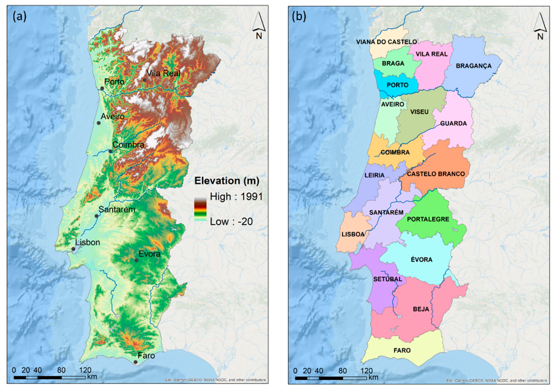
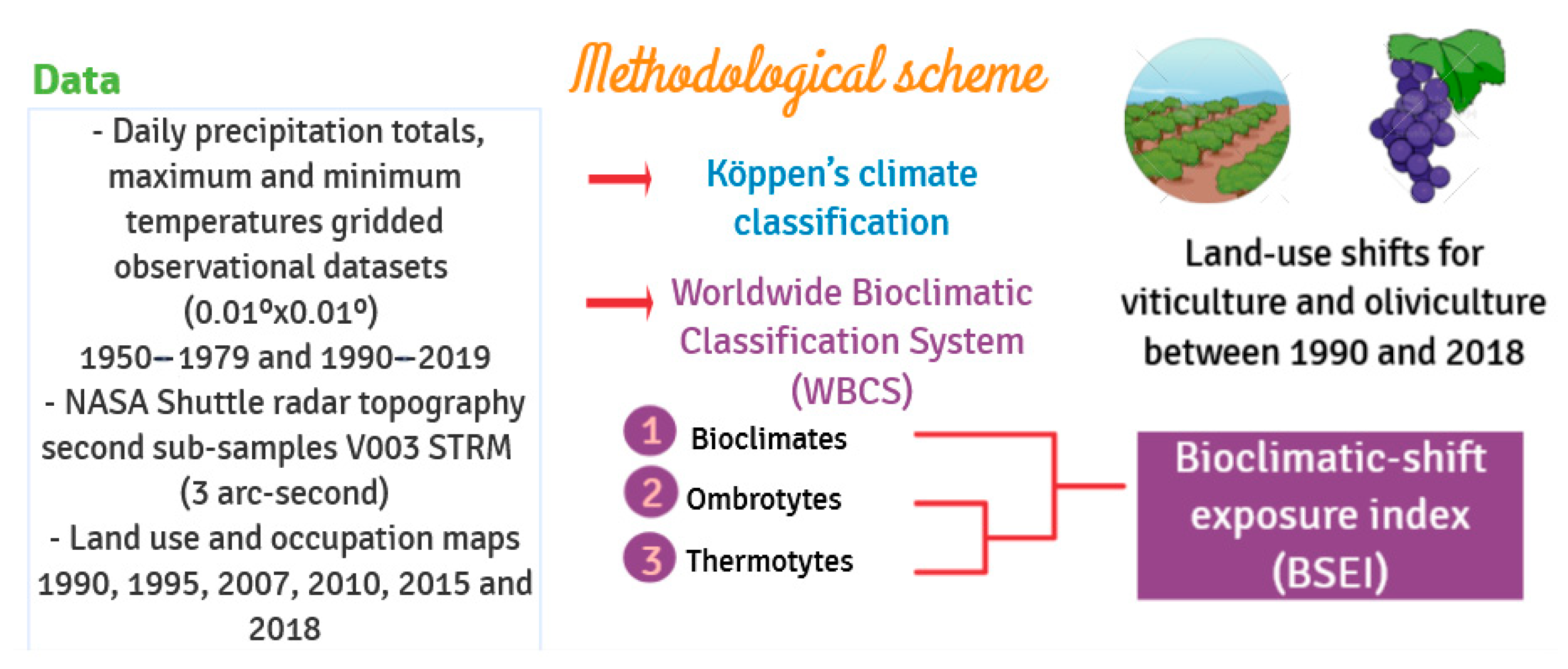
2.1. Data and Study Area

In this study, four high-resolution gridded observational datasets were used between 1950 and 2019. The methodology for the development of this dataset is described by Fonseca and Santos [34]. A two-step approach was carried out: (1) monthly baseline (1971–2000) patterns were estimated at 1-km grid resolution resorting to multivariate linear regressions (exploratory variables: elevation, latitude, and distance to the coastline). Kriging of residuals from baseline normals of a network of weather stations was applied for bias corrections; (2) further, bilinearly interpolated daily temperature anomalies were then added to the daily baseline patterns to obtain the final datasets regarding temperature.
The daily precipitation totals (P, in mm), maximum (TX, in °C), mean (TG, in °C), and minimum (TN, in °C) temperatures, are defined on a 0.01° regular grid. Two 30-year periods were analyzed, i.e., 1950–1979 and 1990–2019, aiming at finding climatic shifts already in progress in mainland Portugal.
The study area is within the geographical sector: 36.95° N–42.16° N and 9.48° W–6.17° W (Figure 1). However, all figures presented herein will be clipped excluding the grid boxes over the Atlantic Ocean. Figure 1a shows a hypsometric chart, with a spatial resolution of 3 arc-second, and was compiled from mosaics retrieved from STRMGL3S Nasa Shuttle radar topography second sub-sampled V003 distributed by (MEaSUREs) SRTM [35]. The area of interest also includes 18 districts in mainland Portugal (Figure 1b). All maps are projected onto the GCS ETRS 1989 Geographical Coordinate System.
The land use and occupation maps were retrieved from https://snig.dgterritorio.gov.pt/ accessed on 30 June 2021 [36], for the years 1990, 1995, 2007, 2010, 2015, and 2018. This satellite-based land cover open access dataset known has the Official Administrative Chart of Portugal (CAOP 2020) is available throughout the country on an annual timescale. For this study, only the spatial representation of monocultures was taken into consideration (vineyards or olive groves separately). The level that presents both vineyards and olive groves land use was disregarded to avoid misleading conclusions. However, the total area evolution for both cultures and the related total amount of production are subsequently presented in tables and graphics between 1989 and 2020 (when available).

2.2. Köppen’s Climate Classification

Köppen’s climate classification is based on a subdivision of major climate types, which are represented by five capital letters, from A to E (considered the main group), followed by two others. In our study, C is used for temperate climates in the mid-latitudes. The second letter identifies the seasonal precipitation type: S for steppe, W desert, while f indicates no dry season. The last letter specifies the level of heat, with a for hot summer, b for warm summer, c for cold summer, d for very cold winter, and h and k are associated with hot and cold climates, respectively. The whole calculation follows the methodology described by Kottek et al. [37] in Tables S1 and S2, whereas the nomenclature (Table S1) and color scheme follow Andrade and Contente [25]. In this study, the concept of high-altitude type (H climates) was not applied. Further details on this methodology can be found in Andrade and Contente [25].

2.3. Worldwide Bioclimatic Classification System (WBCS)

The WBCS includes four major divisions, according to Rivas-Martínez et al. [23,24]. The first division corresponds to the macrobioclimate, which is subsequently split into the other three: bioclimates (Table 1), ombrotypes (Table 2), and thermotypes (Table 3). The major bioclimatic divisions comprise the computation of three additional indices: the continentality index (CI), the annual ombrothermic index (OI), and the thermicity index (TI). However, four additional ombrothermic indices are also computed: the ombrothermic index of the hottest month of the summer quarter (Ios1), the ombrothermic index of the hottest two months of the summer quarter (Ios2), the ombrothermic index of the summer quarter (Ios3) and the ombrothermic index of the 4 months resulting from adding the summer quarter and the month immediately preceding it (Ios4). Further details can be found in Rivas-Martínez et al. [23,24], while a summary of the main equations can be found in Andrade and Contente [11].

2.4. The Bioclimatic-Shift Exposure Index (BSEI)

The compound bioclimatic-shift exposure index (BSEI) is computed by adding the statistically significant differences between the bioclimates, ombrotypes, and thermotypes between 1990–2019, and 1950–1979, respectively. For each difference, two values are attributed, 0 when there is no change, 1 when a change in the climatic type occurs between the two 30-year periods. The three types are equally weighted in the final value of BSEI. This is performed for each grid point within the study area, separately. Therefore, BSEI will vary from 0, indicating regions not exposed to bioclimatic shifts, to 3, signalling regions highly exposed to bioclimatic shifts (changes in the three classifications simultaneously: bioclimatic, ombrotype, and thermotype) (Table 4). Despite its very simple definition, BSEI is a useful tool to assess the degree of change in climatic conditions at a given location/region, i.e., the degree of exposure to climate change.

2.5. Statistical Analysis

For the bioclimates, ombrotypes, and thermotypes, a comparison between a recent past period 1990–2019, and preceding past conditions 1950–1979 (baseline climate) was undertaken. Anomalies (percentage of change) were computed as the differences between the most recent period and the baseline climate. The statistically significant anomalies (S.S.) were assessed by the Mann–Whitney–Wilcoxon test (MWW), at a 5% significance level [38,39], using the 30-year mean values for each period and location of the study area. This nonparametric test assumes equal medians under the null hypothesis (Ho), against the alternative hypothesis (Ha) of different medians.
For each land use and occupation map, the areas of vineyards and olive groves were extracted to assess their spatial-temporal development. Further, the data was compared with the bioclimates, ombrotypes, and thermotypes of the recent period to analyze the shift of land use in both cultivars. The overall methodological schematics of this study can be depicted in Figure 2.

3. Results

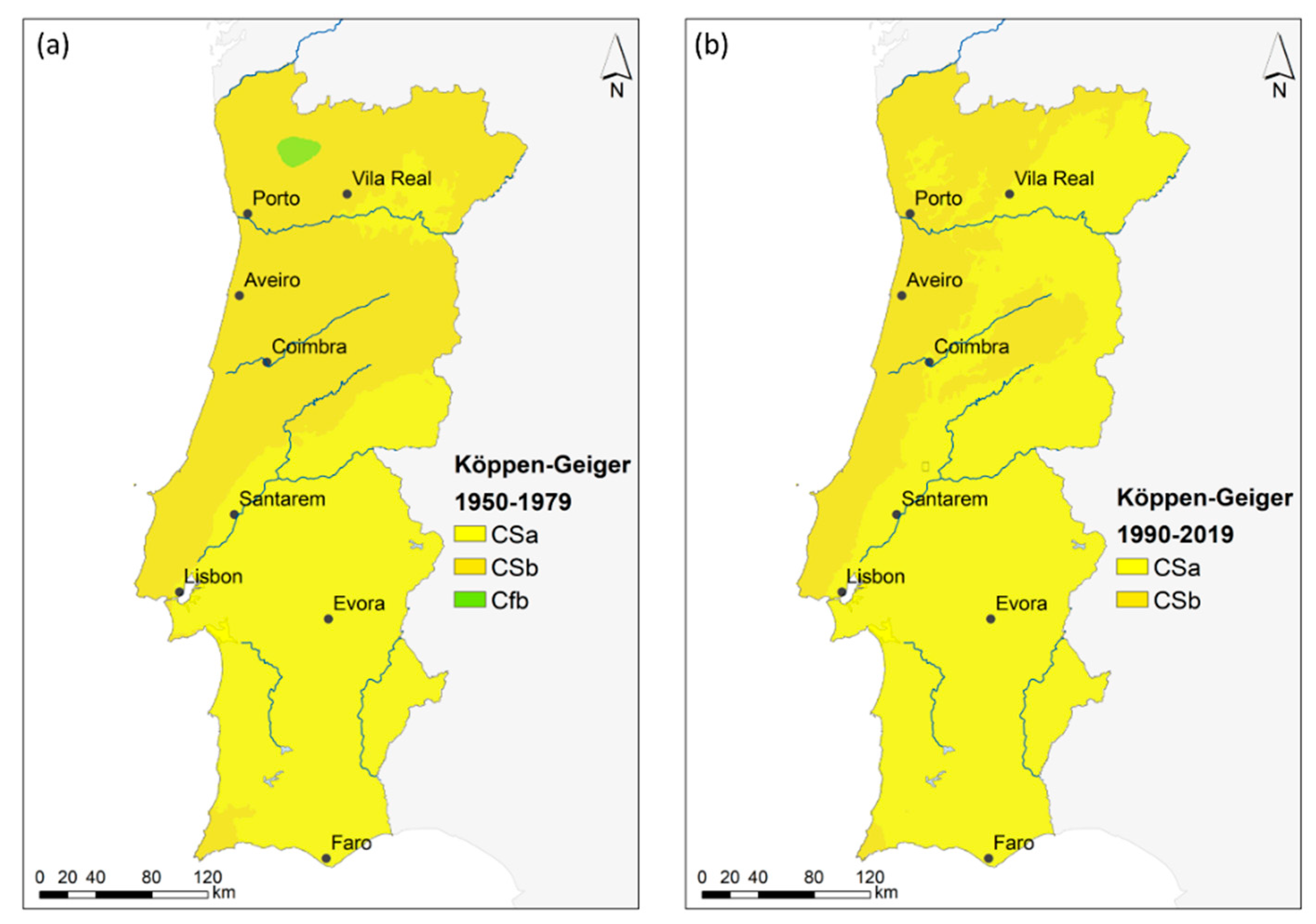
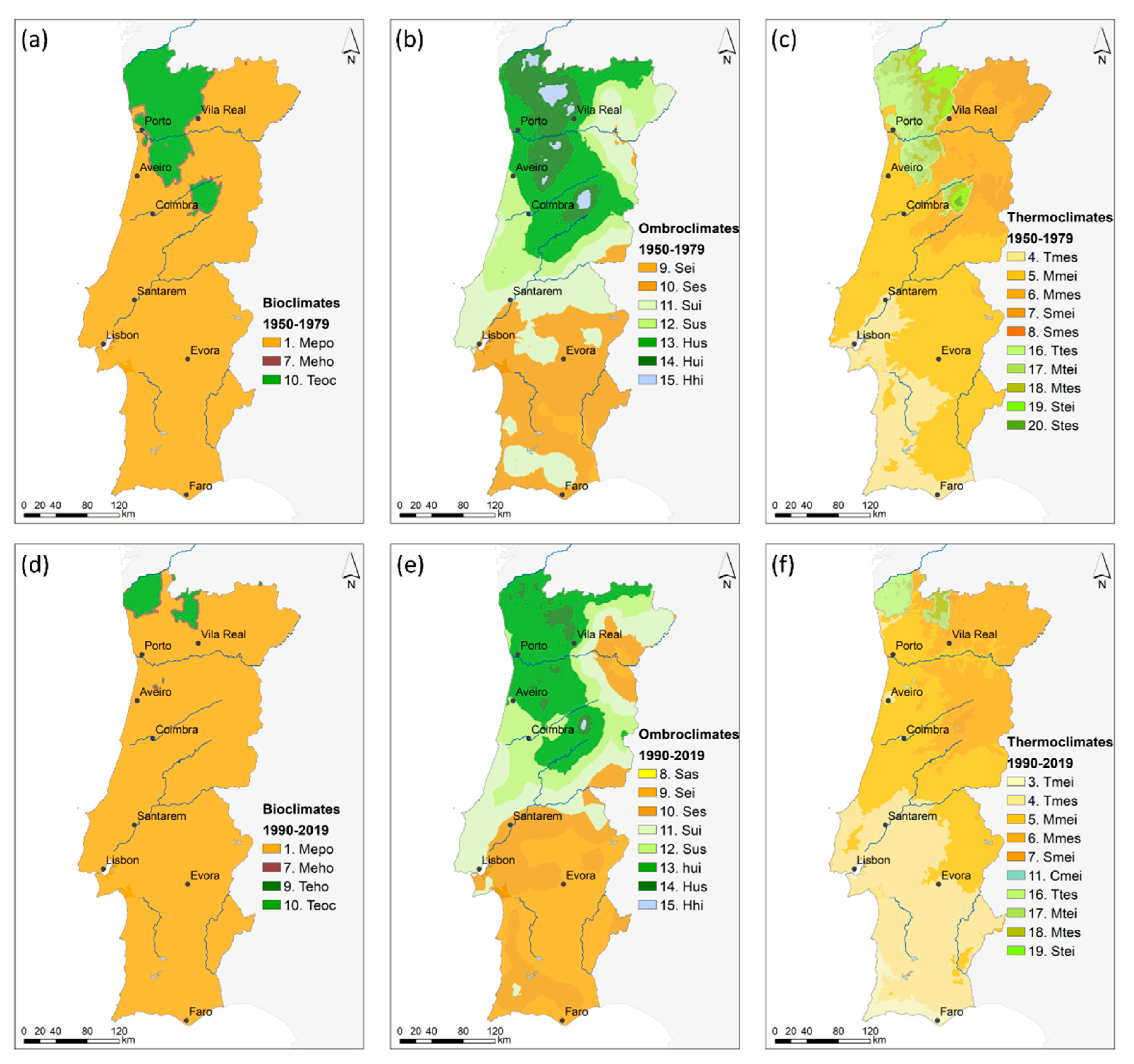
3.1. Köppen–Geiger Climate Classification and WBCS

The spatial representation of the Köppen–Geiger climate classification in mainland Portugal for the period 1950–1979 reveals three climate types (Figure 3a). Two within the CS ‘warm temperate/Mediterranean with dry summer’ and one Cf ‘warm temperate/Mediterranean fully humid’ (Table S1). The prominent climate was CSa (warm temperate/Mediterranean with hot summer) in 53.9% of the territory, CSb (warm temperate/Mediterranean with warm summer) in 45.8%, and only 0.03% for Cfb (warm temperate/Mediterranean fully humid with hot summer) (Table 5, Tables S1 and S2). Besides a small area in the very southwest (Faro district, Figure 1b), the CSb type is mostly found in the northern half of the country, northwards of the Tagus River basin. Conversely, the CSa type is predominant in the southern half, and a small region between the Vila Real and Bragança districts (Figure 1a and Figure 3a). The small area of Cfb climate is located in a mountainous region in the northwest (Figure 1b and Figure 3a).
For 1990–2019, only two types are found (CSa and CSb), with an increase of +18.1% in CSa type (hot summer) and a resulting decrease of −17.8% in CSb (warm summer), a milder climate (Table 5). This later climate type is now depicted along the north-central western coast and in mountainous areas in the northern half of the country.
The changes depicted in the Köppen–Geiger climatic system are also translated for the WBCS classification in which only two macroclimates were found for the two time periods, the Mediterranean and the temperate, which decreased from 1950–1979 to 1990–2019. This can be inferred by observing Figure 4a,d, where the bioclimates are derived from the macroclimates identified by the prefix M for the Mediterranean and T for temperate.
The results also show a transition from three bioclimates in 1950–1979 to four in 1990–2019, though Teho only underwent an increase of +0.03% (Table 6). Nevertheless, the most striking difference is related to the loss of temperate regions (‒5.14%) of Teoc, with an increase of Mepo of +4.78%. These changes have occurred mainly in northwestern Portugal (Figure 4a,d).
Climate change has also affected the ombrotypes. They changed from seven to eight types (Figure 4b,e), with the emergence of a new ombrotype, Sas, within the semi-arid ombrothermic horizons, and corresponding to 0.74% of the territory in 1990–2019 (Table 6). The most relevant changes have occurred for Sei, within the arid ombrothermic horizons with an increase of +24.07%, followed by an overall decrease in almost all humid horizons. The exception was for Sus (upper subhumid), though with a marginal increase of only 1.02% in 1990–2019. Although the Ses (upper dry) ombroclimate area has decreased −13.66%, it is still worth noting the decrease in the percentage of the territory of humid and hyper-humid regions (Sui, Hui, Hus, and Hhi), with an overall total decrease of −12.17% in 1990–2019. These changes have occurred mainly in central (in the vicinity of Serra da Estrela mountainous region) and northwestern Portugal (Figure 4b,e).
Regarding the thermotypes, the findings are consistent with the previous WBCS types. A loss of the territory with temperate thermotypic horizons is verified, e.g., within the thermotemperate (Ttes, −0.91%), mesotemperate (Mtei and Mtes, −2.77 and −1.15%, respectively), and supratemperate (Stei −2.14% and Stes non-existent in 1990–2019) (Table 6). Nonetheless, within the Mediterranean thermotypic horizons, changes were also found. There was a major increase in the thermomediterranean horizons (Tmei and Tmes, +10.74 and +8.16%, respectively), followed by mixed results for the mesomediterranean horizons, with a decrease of −8.10% for Mmei and an increase of +4.74% for Mmes. Lastly, a decrease in the supramediterranean thermotypic horizons are found (Smei and Smes, −8.62 and −0.28%, respectively), as well as the arising of a small region of Cmei (+0.48%) in 1990–2019. The gain of Tmei and Tmes areas (associated with more arid/dry conditions) have occurred mainly in the southern half of the country (Figure 4c,f), whilst the loss of temperate thermotypic horizons was registered in the northwesternmost regions.

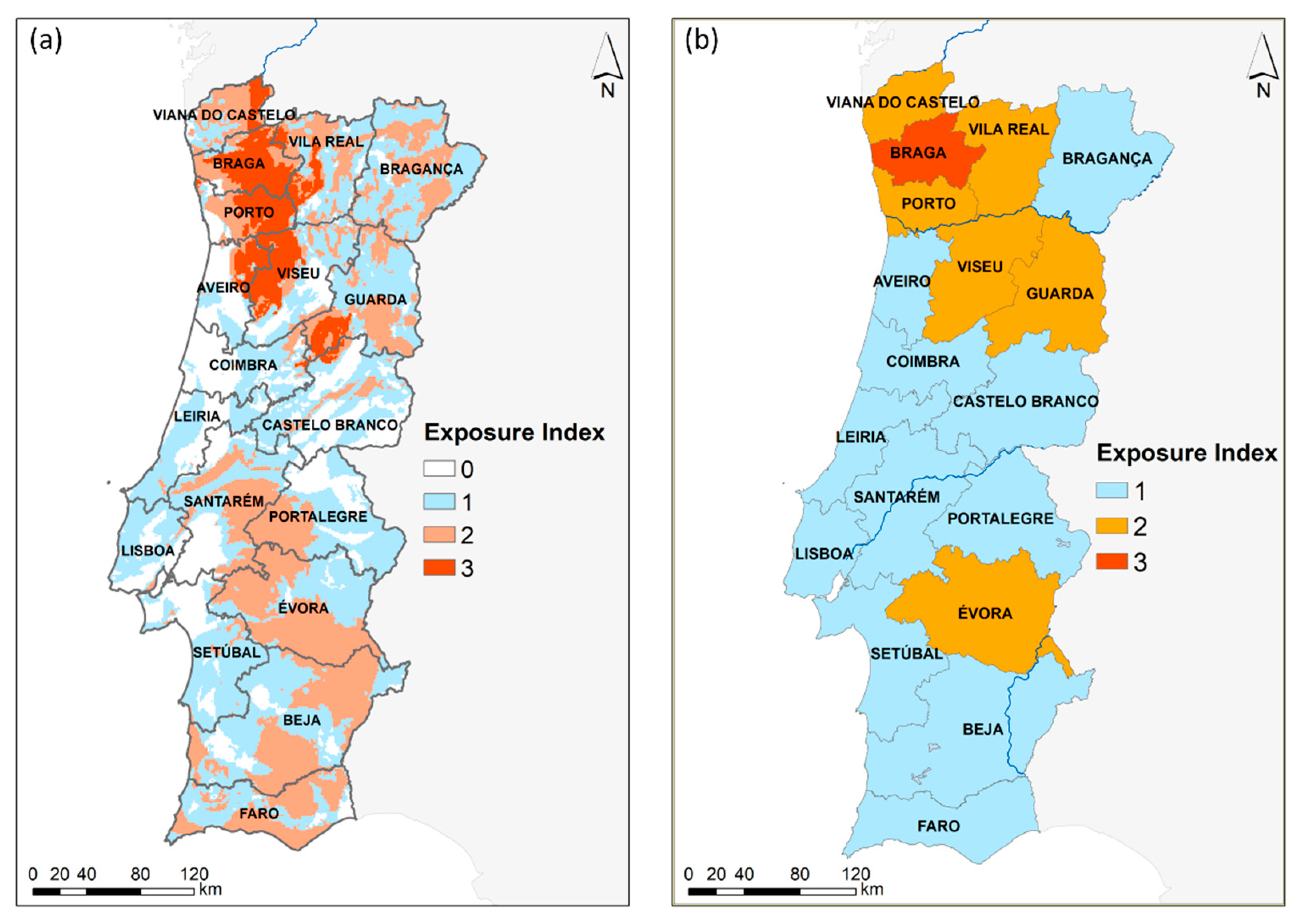
3.2. The Bioclimatic-Shift Expose Index (BSEI)

The BSEI captures the accumulated changes that have occurred between 1990–2019 and 1950–1979 between bioclimates, ombrotypes, and thermotypes. Thus, it captures the most exposed regions to the bioclimatic shifts analyzed in the previous sub-section. Regions with no changes have a zero score, while regions with changes in the three WBCS indicators have a score of three. Figure 5a depicts the highest exposures (BSEI = 3, highly exposed) in Viana do Castelo, Braga, Porto, Aveiro, Viseu, and Guarda districts. These outcomes are consistent with both the loss of temperate regions and the increase of more arid/dry bioclimatic types in the former regions (Figure 4). Large areas with BSEI = 2 (moderately exposed) can still be found in the aforementioned districts, as well as in the northeast (Bragança). On the other hand, in the southern half of the country, BSEI = 2 can be found in the Santarém, Portalegre, Évora, Beja, and Faro districts (Figure 5a). In these latter regions, however, changes are mostly due to shifts in the ombrotypes and thermotypes (Figure 4b,c,e,f).
For a better understanding of the extent of exposure to the bioclimatic shifts, the areal mean values for each district were computed. The Braga district is the most exposed (BSEI = 3), followed by Viana do Castelo, Vila Real, Porto, Viseu, Guarda, and Évora districts, all of them with BSEI = 2 (Figure 5b). All the remaining districts have BSEI = 1 (weakly exposed).

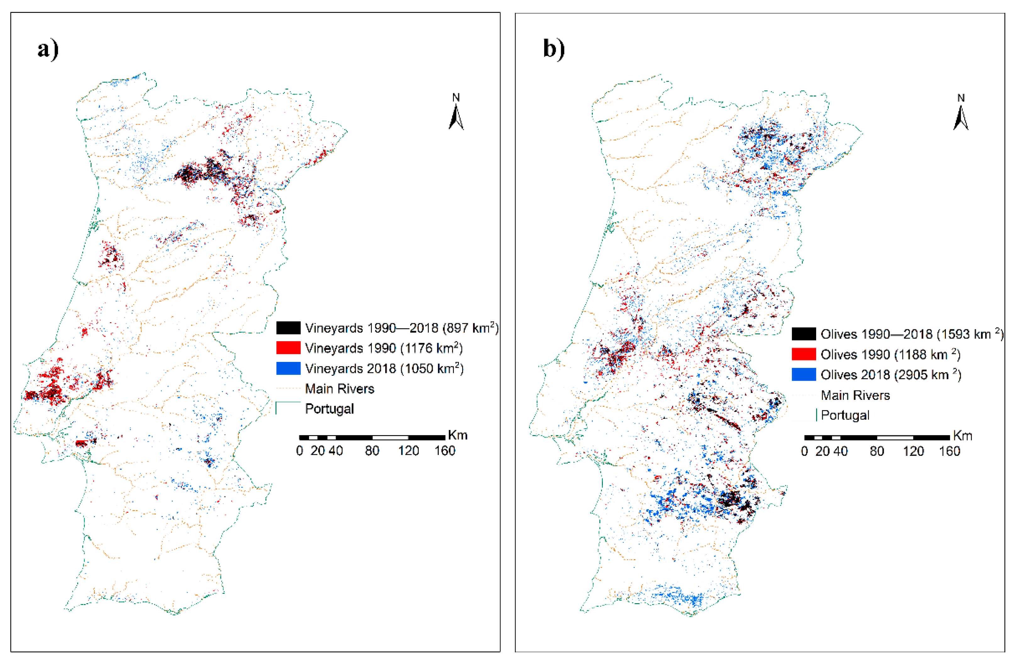
3.3. Land-Use Changes for Viticulture and Oliviculture from 1990 to 2018

The vineyard cover area in Portugal has decreased from 1990 to 2018 (only land use levels for monocultures were considered). The decrease is approximately 6% (126 km2) (Figure 6a), mainly in the Lisboa district. New vineyard cover areas are, however, observed in Alentejo (mostly Évora district) and in northwestern Portugal, which are in both cases areas with higher BSEI values. For the olive groves, the area has significantly increased by approximately 62% (1717 km2) (Figure 6b), mainly in Faro, Beja, Vila Real, and Bragança districts, among which only Vila Real shows a higher BSEI (2, moderate exposure).
Concerning the evolution of the growing bioclimatic conditions in the vineyard cover area from 1990 to 2018 (Figure 7a), there is a shift towards new regions that are both humid (Hui), in northwestern Portugal (Vinho Verde WR), and dry (Sei), in southern Portugal (Alentejo WR) (Figure S1). Conversely, a decrease in the areas classified as subhumid (Sus and Sui) is also apparent. Hence, vineyards are gradually occupying more extremes conditions in terms of climate humidity. The change in thermotype conditions of vineyards areas is not statistically significant (Figure 7c).
For the temporal evolution in land use for olive groves, there is a general trend for a shift towards more humid (an increase of cover area in classes Hui and Hus) and cooler areas (increase in Mmes and decreases in the warmer classes of Mmei and Tmes).

4. Discussion

The present climatic characterization aimed at identifying the regions in mainland Portugal that have endured the most significant bioclimatic shifts from 1950–1979 to 1990–2019. Most of the areas or districts that experienced more accentuated alterations in the bioclimatic classes from one period to the other are located in northwestern Portugal. For the second period (1990–2019), satellite-based land cover data are available throughout the country on an annual timescale. Therefore, the evolution of vineyard and olive grove areas was analyzed to assess to what extent have these crops been expanded to more susceptible zones to bioclimatic shifts. To our knowledge, there are no related studies regarding oliviculture and viticulture that use the Köppen–Geiger climatic classification, the WBCS, as well as the compound BSEI to evaluate the bioclimatic shifts. Therefore, it was not possible to compare the methodology used in this study since there are no similar cases for comparison.
The evolution in the vineyard cover area from 1990 to 2018 (Figure 7a) shows a bidirectional displacement, towards the regions with more extreme bioclimates in the territory. The vineyard area has been increasing in the relatively cool and humid regions of northwestern Portugal (Vinho Verde WR), as well as in the warm and dry regions of southern Portugal (Alentejo WR) (Figure S1). In effect, from 2018 to 2020, vineyard areas have increased in the north, e.g., in Minho 2267 ha, in Douro/Porto 3212 ha, but also southern Portugal, in Alentejo VR 513 ha (Table S3). These regions are, nevertheless, located in areas for which the BSEI indicates stronger bioclimatic shifts during the last decades (Minho WR, Douro/Porto WR, and Alentejo WR). Even though the increase in the vineyard area in regions with cooler and more humid climates can be considered a climate-smart adaptation strategy, thus enhancing the climate resilience of the sector, the pronounced bioclimatic shifts observed in these regions may considerably affect the regional terroirs and, as a result, the wine typicity and style [40]. In addition, the emergence of vast areas with irrigated vineyards under the typically warm and dry conditions of southern Portugal will threaten the already limited water resources [41], thereby requiring more efficient water management and water-saving agricultural practices. The lack of water availability may indeed challenge the future sustainability of the sector in this region. This will be particularly relevant under the projected future warmer and drier climates, which will exacerbate the current warm and dry conditions, becoming irrigation even more vital [20].
As for viticulture, the olive grove land cover in Portugal has been changing between 1990 and 2018 (Figure S3). These fluctuations have also impacted olive yield, which was approximately 700,000 t in 2019 (Figure S4). The recent area expansion occurred mainly in the Faro, Beja, Vila Real, and Bragança districts, the last two showing relatively high BSEI (Figure 6b). Regions in the north are indeed gradually experiencing climatic conditions that were more typical of southern Portugal a few decades ago and are, thereby, becoming more suitable for oliviculture. Although the area of olive groves has undergone a significant increase in southern Portugal, most of them irrigated, the progressively higher relative coverage in cooler climates, still predominantly rainfed orchards, may already suggest higher awareness and a more or less conscious attempt of the sector to adapt to the ongoing climate change. It is worth mention that the construction of the Alqueva dam in the Guadiana River, which has created one of the biggest artificial lakes in Europe had a huge impact in the inner southern region of mainland Portugal. The increase in the regional water resources, allowed the implementation of a wide water distribution and irrigation systems. This fact influenced the expansion of vineyards and olive groves, among other cultures in this region during the timeframe analyzed in this study.

5. Conclusions

The present study assessed the climate change trends that have already influenced the Köppen–Geiger climate classification and the WBCS between 1950 and 2019 in mainland Portugal. For this purpose, a comparison between two 30-year periods, i.e., 1950–1979 and 1990–2019, was undertaken for these two climate classifications. It is worth mentioning that these calculations were carried out using high-resolution gridded datasets, with approximately 1 km grid resolution, thus providing accurate and detailed information throughout the country. To our knowledge, this is the first study analyzing these climate classifications in Portugal at such a high resolution.
The spatial representation of the Köppen–Geiger climate classification revealed three climate types (Figure 3a) in 1950–1979. The leading climate type was CSa, in 53.9% of the territory, CSb in 45.8%, and a very small percentage of 0.03% for Cfb. The CSa type was predominant in the southern half of Portugal and a narrow region in the south of the Vila Real and Bragança districts (Figure 1a and Figure 3a). The CSb was dominant throughout most of the northern half of Portugal, mostly northwards of the Tagus River basin. However, a clear bioclimatic shift in 1990–2019 was detected, with an increase of +18.1% in CSa type, associated with hot summers, and a corresponding decrease of −17.8% in CSb, associated with warm summers, and therefore, a milder climate (Table 5). These findings are in general agreement with Andrade and Contente [25].
The results also hint at shifts in the WBCS four major divisions from 1950–1979 to 1990–2019, related to a decrease of −5.11% in the temperate macroclimate in the northwest, followed by an increase in the Mediterranean macroclimate. This change impacted the bioclimates since a transition from three bioclimates in 1950–1979 to four bioclimates in 1990–2019 was identified, with the decrease of −5.14% for Teoc, counterbalanced by an increase of +4.78% for Mepo. As previously, these changes have occurred mainly in the northwestern regions of Portugal (Figure 4a,d). The ombrotypes changed from seven to eight types (Figure 4b,e), with a new ombrotype, Sas, within the semi-arid ombrothermic horizons, corresponding to +0.74% of the territory in 1990–2019 (Table 6). The overall decrease of −12.17% in the percentage of the territory of humid and hyper-humid regions (Sui, Hui, Hus and Hhi), in detriment of an increase of +24.81% of semi-arid and arid for 1990–2019, is particularly noteworthy.
For the thermotypes, a loss of 7.12% in the percentage of the territory associated with all temperate thermotypic horizons was found (Table 6). Within the Mediterranean thermotypic horizons, changes were also found. There was a major increase in the thermomediterranean horizons of +18.9%. For the mesomediterranean horizons, a decrease of −8.10% for Mmei, an increase of +4.74% for Mmes, followed by a loss of −8.9% in supramediterranean thermotypic horizons were identified in 1990–2019. Overall, in the southern half of the country (Figure 4c,f), a gain of thermomediterranean horizons, associated with more arid/dry conditions, was observed. On the other hand, the loss of both Mediterranean and temperate thermotypic horizons, with milder conditions, was registered in the northwesternmost regions. Climate shifts were observed in the major divisions of the WBCS classification are in clear accordance with the study of Andrade and Contente [11] for the IP. The changes in WBCS have direct implications in the regional exposure to bioclimatic shifts, measured by BSEI. At the district level, the Braga district (in the northwest) is the most exposed (BSEI = 3), followed by Viana do Castelo, Vila Real, Porto, also in the north, Viseu and Guarda in the center; and Évora in the south (BSEI = 2).
For both grapevines and olive trees, which are major crops in Portugal, the results highlight the growth in their land cover areas in southern regions that are becoming dryer. Furthermore, the vineyard area is increasing in the northwest, in regions that present higher values of BSEI, hence more exposed to recent past bioclimatic shifts. This may significantly affect the regional terroirs, grape berry attributes, and wine typicity and style. Conversely, the relative share of southern Portugal to the total olive grove area has been decreasing, which may already suggest an adaptation strategy of the sector, by progressively relocating olive orchards in northern regions that are currently experiencing similar conditions to those found in southern regions a few decades ago.
Both viticulture and oliviculture may be particularly challenged under future climate change scenarios, as suggested by Fraga et al. [20] for viticulture in Portugal, or by Fraga et al. [42] and Fraga et al. [43] for olive yields in Portugal and the Mediterranean region, respectively. As a result, better planning of the distribution of these key crops in Portugal should be envisioned, avoiding the increasing dependence on irrigation, which will eventually disrupt local and regional surface and underground water resources [44]. New agricultural practices and options are urging to enhance the water use efficiency of crops [45]. New water-saving and go-green policies and strategies will be particularly relevant under the projected future warmer and drier climates in Portugal [40,46]. On the other hand, warranting the future environmental and socio-economic sustainability of these sectors is of foremost relevance for the national economy and food security, thereby deserving further research. As similar problems can be found in many other regions with Mediterranean-type climates, the main outcomes from this study can be easily extrapolated to other countries worldwide.

Supplementary Materials

The following are available online at https://www.mdpi.com/article/10.3390/land10080869/s1, Table S1: Criteria to calculate the Köppen-Geiger classification for the main climates and subsequent precipitation conditions for the first two letters. For the polar climates (E) no precipitation differentiations are given, only temperature conditions are defined, consequently, the polar climates (E) must be determined first, followed by the arid climates (B) and subsequent differentiation into the equatorial climates (A) and the warm temperate and snow climates (C) and (D), respectively; Table S2: Criteria for the third letter temperature classification (h and k) for dry climates (B) and (a to d) for the warm temperate (C) and continental (D) climates following the Köppen’s climate classification; Table S3: Vineyard land cover evolution (in ha) over mainland Portugal, by Wine Region; Figure S1: Viticulture regions (IGP or VR) in mainland Portugal with the associated Control origin denomination (DOC); Figure S2: Evolution of the total wine production (in hl) by viticulture region and subtotal for mainland Portugal for 2009, 2018/19, 2019/20, and 2020/21; Figure S3: Evolution of the total olive grove areas (in ha) for mainland Portugal between 1990 and 2018; Figure S4: Evolution of the total olive production (in ton) for mainland Portugal between 2000 and 2020.

Author Contributions

For this research, the author’s contributions were: conceptualization, C.A. and J.A.S.; methodology, C.A. and J.A.S.; software, C.A. and A.F.; validation, C.A. and J.A.S.; formal analysis, C.A., A.F., J.A.S.; investigation, C.A., A.F., J.A.S.; resources, C.A. and A.F.; data curation, C.A. and A.F.; writing—C.A.; writing—C.A. and J.A.S.; visualization, C.A. and A.F.; supervision, C.A. and J.A.S.; project administration, J.A.S.; funding acquisition, J.A.S. All authors have read and agreed to the published version of the manuscript.

Funding

This study was funded by the European Commission-funded project “Climate Change Impact Mitigation for European Viticulture: Knowledge Transfer for an Integrated Approach—Clim4Vitis” [grant 810176]. This research was also supported by National Funds from FCT—Portuguese Foundation for Science and Technology, under the project UIDB/04033/2020.

Institutional Review Board Statement

Not applicable.

Informed Consent Statement

Not applicable.

Data Availability Statement

Not applicable.

Conflicts of Interest

The authors declare no conflict of interest.

References

  1. Climate Change and Land, An IPCC Special Report on Climate Change, Desertification, Land Degradation, Sustainable Land Management, Food Security, and Greenhouse gas fluxes in Terrestrial Ecosystems, Summary for policymakers. 2019. Available online: https://www.ipcc.ch/srccl/ (accessed on 9 July 2021).
  2. Tasser, E.; Leitinger, G.; Tappeiner, U. Climate Change versus Land-Use Change—What Affects the Mountain Landscapes More? Land Use Policy 2017, 60, 60–72. [Google Scholar] [CrossRef]
  3. Ellis, E.C. Sustaining biodiversity and people in the world’s anthropogenic biomes. Environ. Sustain. 2013, 5, 368–372. [Google Scholar] [CrossRef]
  4. Martins, I.S.; Proença, V.; Pereira, H.M. The unusual suspect: Land use is a key predictor of biodiversity patterns in the Iberian Peninsula. Acta Oecol. 2014, 61, 41–50. [Google Scholar] [CrossRef] [Green Version]
  5. Haberl, H.; Erb, K.H.; Krausmann, F.; Gaube, V.; Bondeau, A.; Plutzar, C.; Gingrich, S.; Lucht, W.; Fischer-Kowalski, M. Quantifying and mapping the human appropriation of net primary production in earth’s terrestrial ecosystems. Proc. Natl. Acad. Sci. USA 2007, 104, 12942–12947. [Google Scholar] [CrossRef] [PubMed] [Green Version]
  6. Fernández-Nogueira, D.; Corbelle-Rico, E. Land Use Changes in Iberian Peninsula 1990–2012. Land 2018, 7, 99. [Google Scholar] [CrossRef] [Green Version]
  7. Van Vliet, J.; de Groot, H.L.F.; Rietveld, P.; Verburg, P.H. Manifestations and Underlying Drivers of Agricultural Land Use Change in Europe. Landsc. Urban Plan. 2015, 133, 24–36. [Google Scholar] [CrossRef] [Green Version]
  8. Levers, C.; Butsic, V.; Verburg, P.H.; Müller, D.; Kuemmerle, T. Drivers of Changes in Agricultural Intensity in Europe. Land Use Policy 2016, 58, 380–393. [Google Scholar] [CrossRef] [Green Version]
  9. De Chazal, J.; Rounsevell, M.D.A. Land-Use and Climate Change within Assessments of Biodiversity Change: A Review. Glob. Environ. Chang. 2009, 19, 306–315. [Google Scholar] [CrossRef]
  10. Lindner, M.; Maroschek, M.; Netherer, S.; Kremer, A.; Barbati, A.; Garcia-Gonzalo, J.; Seidl, R.; Delzon, S.; Corona, P.; Kolström, M.; et al. Climate Change Impacts, Adaptive Capacity, and Vulnerability of European Forest Ecosystems. For. Ecol. Manag. 2010, 259, 698–709. [Google Scholar] [CrossRef]
  11. Andrade, C.; Contente, J. Climate change projections for the Worldwide Bioclimatic Classification System in the Iberian Peninsula until 2070. Int. J. Climatol. 2020, 40, 5863–5886. [Google Scholar] [CrossRef]
  12. Diffenbaugh, N.S.; Pal, J.S.; Giorgi, F.; Gao, X. Heat Stress Intensification in the Mediterranean Climate Change Hotspot. Geophys. Res. Lett. 2007, 34. [Google Scholar] [CrossRef] [Green Version]
  13. Diffenbaugh, N.S.; Giorgi, F. Climate Change Hotspots in the CMIP5 Global Climate Model Ensemble. Clim. Chang. 2012, 114, 813–822. [Google Scholar] [CrossRef] [Green Version]
  14. Andrade, C.; Leite, S.M.; Santos, J.A. Temperature Extremes in Europe: Overview of Their Driving Atmospheric Patterns. Nat. Hazards Earth Syst. Sci. 2012, 12, 1671–1691. [Google Scholar] [CrossRef] [Green Version]
  15. Andrade, C.; Contente, J.; Santos, J.A. Climate Change Projections of Dry and Wet Events in Iberia Based on the WASP-Index. Climate 2021, 9, 94. [Google Scholar] [CrossRef]
  16. Santos, J.A.; Belo-Pereira, M.; Fraga, H.; Pinto, J.G. Understanding Climate Change Projections for Precipitation over Western Europe with a Weather Typing Approach. J. Geophys. Res. Atmos. 2016, 121, 1170–1189. [Google Scholar] [CrossRef] [Green Version]
  17. Santos, M.; Fonseca, A.; Fragoso, M.; Santos, J.A. Recent and Future Changes of Precipitation Extremes in Mainland Portugal. Theor. Appl. Climatol. 2019, 137, 1305–1319. [Google Scholar] [CrossRef]
  18. Scoccimarro, E.; Villarini, G.; Vichi, M.; Zampieri, M.; Fogli, P.G.; Bellucci, A.; Gualdi, S. Projected Changes in Intense Precipitation over Europe at the Daily and Subdaily Time Scales. J. Clim. 2015, 28, 6193–6203. [Google Scholar] [CrossRef]
  19. Vidal-Macua, J.J.; Ninyerola, M.; Zabala, A.; Domingo-Marimon, C.; Gonzalez-Guerrero, O.; Pons, X. Environmental and socioeconomic factors of abandonment of rainfed and irrigated crops in northeast Spain. Appl. Geogr. 2018, 90, 155–174. [Google Scholar] [CrossRef]
  20. Fraga, H.; de Cortázar Atauri, I.G.; Santos, J.A. Viticultural Irrigation Demands under Climate Change Scenarios in Portugal. Agric. Water Manag. 2018, 196, 66–74. [Google Scholar] [CrossRef]
  21. Fraga, H.; Santos, J.A. Assessment of Climate Change Impacts on Chilling and forcing for the Main Fresh Fruit Regions in Portugal. Front. Plant. Sci. 2021. [Google Scholar] [CrossRef]
  22. Köppen, W.; Geiger, R. Handbuch der Klimatologie; Gebrüder Bornträger: Berlin, Germany, 1930; Volume 6. [Google Scholar]
  23. Rivas-Martínez, S.; Sáenz, S.R.; Penas, A. Worldwide bioclimatic classification system. Glob. Geobot. 2011, 1, 1–634. [Google Scholar] [CrossRef]
  24. Rivas-Martínez, S.; Penas, A.; del Río, S.; González, T.; Rivas-Sáenz, S. Bioclimatology of the Iberian Peninsula and the Balearic Islands. In The Vegetation of the Iberian Peninsula.Plant and Vegetation; Loidi, J., Ed.; Springer: Cham, Switzerland, 2017; Volume 12. [Google Scholar] [CrossRef]
  25. Andrade, C.; Contente, J. Köppen’s climate classification projections for the Iberian Peninsula. Clim. Res. 2020, 81, 71–89. [Google Scholar] [CrossRef]
  26. Fernández-Nogueira, D.; Corbelle-Rico, E. Determinants of Land Use/Cover Change in the Iberian Peninsula (1990‒2012) at Municipal Level. Land 2019, 9, 5. [Google Scholar] [CrossRef] [Green Version]
  27. Turpin, N.; Berge, H.T.; Grignani, C.; Guzmán, G.; Vanderlinden, K.; Steinmann, H.H.; Siebielec, G.; Spiegel, H.; Perret, E.; Ruysschaert, G.; et al. An Assessment of Policies Affecting Sustainable Soil Management in Europe and Selected Member States. Land Use Policy 2017, 66, 241–249. [Google Scholar] [CrossRef]
  28. Jones, N.; de Graaff, J.; Rodrigo, I.; Duarte, F. Historical Review of Land Use Changes in Portugal (before and after EU Integration in 1986) and Their Implications for Land Degradation and Conservation, with a Focus on Centro and Alentejo Regions. Appl. Geogr. 2011, 31, 1036–1048. [Google Scholar] [CrossRef]
  29. Available online: https://www.ivv.gov.pt/np4/499/ (accessed on 30 June 2021).
  30. Available online: https://www.oiv.int/public/medias/7909/oiv-state-of-the-world-vitivinicultural-sector-in-2020.pdf (accessed on 9 July 2021).
  31. Available online: https://www.ivv.gov.pt/np4/7179.html (accessed on 9 July 2021).
  32. Available online: https://www.ivv.gov.pt/np4/163.html (accessed on 9 July 2021).
  33. Available online: https://www.gpp.pt/images/PEPAC/Anexo_NDICE_ANLISE_SETORIAL___AZEITE.pdf (accessed on 30 June 2021).
  34. Fonseca, A.R.; Santos, J.A. High-resolution temperature datasets in Portugal from a geostatistical approach: Variability and extremes. J. Appl. Meteorol. Climatol. 2018, 57, 627–644. [Google Scholar] [CrossRef]
  35. NASA. NASA Shuttle Radar Topography Mission Global 3 Arc Second Subsampled [Data Set]. Available online: https://lpdaac.usgs.gov/products/srtmgl3v003/ (accessed on 17 August 2021).
  36. Available online: https://snig.dgterritorio.gov.pt/ (accessed on 30 June 2021).
  37. Kottek, M.J.; Grieser, C.; Beck, B.; Rudolf, R. World map of the Köppen–Geiger climate classification updated. Meteorol. Z. 2006, 15, 259–263. [Google Scholar] [CrossRef]
  38. Wilcoxon, F. Individual comparisons by ranking methods. Biom. Bull. 1945, 1, 80–83. [Google Scholar] [CrossRef]
  39. Mann, H.B. Non-parametric tests against trend. Econometrica 1945, 13, 245–259. [Google Scholar] [CrossRef]
  40. Santos, J.A.; Fraga, H.; Malheiro, A.C.; Moutinho-Pereira, J.; Dinis, L.-T.; Correia, C.; Moriondo, M.; Leolini, L.; Dibari, C.; Costafreda-Aumedes, S.; et al. A review of the Potential Climate Change Impacts and Adaptation options for European Viticulture. Appl. Sci. 2020, 10, 3092. [Google Scholar] [CrossRef]
  41. Costa, J.M.; Oliveira, M.; Egipto, R.J.; Cid, R.J.; Fragoso, R.A.; Lopes, C.M.; Duarte, E.N. Water and Wastewater management for sustainable viticulture and oenology in south Portugal–A review. Ciência Téc. Vitiv. 2020, 35, 1–15. [Google Scholar] [CrossRef]
  42. Fraga, H.; Pinto, J.G.; Viola, F.; Santos, J.A. Climate Change Projections for Olive Yields in the Mediterranean Basin. Int. J. Climatol. 2020, 40, 769–781. [Google Scholar] [CrossRef] [Green Version]
  43. Fraga, H.; Moriondo, M.; Leolini, L.; Santos, J.A. Mediterranean Olive Orchards under Climate Change: A Review of Future Impacts and Adaptation Strategies. Agronomy 2021, 11, 56. [Google Scholar] [CrossRef]
  44. Oliveira, M.; Costa, J.M.; Fragoso, R.; Duarte, E. Challenges for modern wine production in dry areas: Dedicated indicators to preview wastewater flows. Water Supply 2019, 19, 653–661. [Google Scholar] [CrossRef]
  45. Martins, A.A.; Araújo, A.R.; Graça, A.; Caetano, N.S.; Mata, T.M. Towards sustainable wine: Comparison of two Portuguese wines. J. Clean Prod. 2018, 183, 662–676. [Google Scholar] [CrossRef]
  46. Fraga, H.; Malheiro, A.C.; Moutinho-Pereira, J.; Santos, J.A. Future scenarios for viticulture zoning in Europe: Ensemble projections and uncertainties. Int. J. Biometeorol. 2013, 57, 909–925. [Google Scholar] [CrossRef]
Figure 1. Mainland Portugal (a) elevation (in m) and (b) the related 18 districts.
Land 10 00869 g001
Figure 2. Methodological schematics of this study.
Land 10 00869 g002
Figure 3. Köppen–Geiger climate classification for (a) 1950–1979 and (b) 1990–2019.
Land 10 00869 g003
Figure 4. Classification for (a) bioclimates; (b) ombrotypes; and (c) thermotypes between 1950–1979 and (df) the same as for (ac) but between 1990–2019.
Land 10 00869 g004
Figure 5. (a) Bioclimatic-shift exposure index (BSEI) for mainland Portugal and (b) related areal mean values for each district (note: BSEI attained between 1990–2019 and 1950–1979).
Land 10 00869 g005
Figure 6. Spatial representation and related area (in km2) of (a) vineyards and (b) olive groves in Portugal for the period between 1990 and 2018. Areas maintained throughout the period in black (persistent areas), only for 1990 in red (discontinued areas), and 2018 in blue (emerging areas).
Land 10 00869 g006
Figure 7. Percentage area regarding each land use and occupation map for vineyards (a,c) and olive groves (b,d) according to each specific climatic classification: (a,b) ombrotype and (c,d) thermotype for the recent past period (1990–2019).
Land 10 00869 g007
Table 1. Bioclimatic classification for Mediterranean and temperate macrobioclimates, according to Rivas-Martínez et al. [23] (Adapted with permission from Andrade and Contente [11]).
Bioclimates Abbr. CI 1 OI 1
1. Mediterranean pluviseasonal oceanic Mepo≤21>2.0
2. Mediterranean pluviseasonal continental Mepc>21>2.0
3. Mediterranean xeric oceanic Mexo≤211.0–2.0
4. Mediterranean xeric continental Mexc>211.0–2.0
5. Mediterranean desertic oceanic Medo≤210.2–1.0
6. Mediterranean desertic continental Medc>210.2–1.0
7. Mediterranean hyperdesertic oceanic Meho≤21<0.2
8. Mediterranean hyperdesertic continental Mehc>21<0.2
9. Temperate hyperoceanic Teho≤11>3.6
10. Temperate oceanic Teoc11–21>3.6
11. Temperate continental Teco>21>3.6
12. Temperate xeric Texe≥4≤3.6
1 In this Table, CI is the continentality index and OI is the ombrothermic index.
Table 2. Ombrothermic horizons, according to Rivas-Martínez et al. [23] Adapted with permission from Andrade and Contente [11]).
Ombrothermic Horizons Abbr. OI 1
1. Lower ultrahyperarid Uhai0.0–0.1
2. Upper ultrahyperarid Uhas0.1–0.2
3. Lower hyperarid Hai0.2–0.3
4. Upper hyperarid Has0.3–0.4
5. Lower arid Ari0.4–0.7
6. Upper arid Ars0.7–1.0
7. Lower semiarid Sai1.0–1.5
8. Upper semiarid Sas1.5–2.0
9. Lower dry Sei2.0–2.8
10. Upper dry Ses2.8–3.6
11. Lower subhumid Sui3.6–4.8
12. Upper subhumid Sus4.8–6.0
13. Lower humid Hui6.0–9.0
14. Upper humid Hus9.0–12.0
15. Lower hyperhumid Hhi12.0–18.0
16. Upper hyperhumid Hhs18.0–24.0
17. Ultrahyperhumid Uhu>24.0
1 In this Table, OI is the ombrothermic index.
Table 3. Thermotypic horizons, to Mediterranean and temperate macrobioclimates. Tp is only used if CI ≥ 21, or TI, TIc < 120, according to Rivas-Martínez et al. [23] (Adapted with permission from Andrade and Contente [11]).
Thermotypic Horizons Abbr. TI 1, Tic 1 Tp 1
1. Lower inframediterranean Imei515–580>2600
2. Upper inframediterranean Imes450–5152400–2600
3. Lower thermomediterranean Tmei400–4502250–2400
4. Upper thermomediterranean Tmes350–4002100–2250
5. Lower mesomediterranean Mmei285–3501800–2100
6. Upper mesomediterranean Mmes220–2851500–1800
7. Lower supramediterranean Smei150–2201200–1500
8. Upper supramediterranean Smes120–150900–1200
9. Lower oromediterranean Omei675–900
10. Upper oromediterranean Omes450–675
11. Lower crioromediterranean Cmei100–450
12. Upper crioromediterranean Cmes1–100
13. Pergelid Gme0
14. Infratemperate Ite>410>2351
15. Lower thermotemperate Ttei350–4102176–2350
16. Upper thermotemperate Ttes290–3502000–2175
17. Lower mesotemperate Mtei240–2901700–2000
18. Upper mesotemperate Mtes190–2401400–1700
19. Lower supratemperate Stei120–1901100–1400
20. Upper supratemperate Stes800–1100
21. Lower orotemperate Otei590–800
22. Upper orotemperate Otes380–590
23. Lower criorotemperate Ctei100–380
24. Upper criorotemperate Ctes1–100
25. Pergelid Gme0
1 In this Table, CI is the continentality index, TI is the thermicity index and TIc is the compensated thermicity index, Tp is the annual positive temperature (tenths of °C), when the mean monthly temperature is higher than 0 °C.
Table 4. Bioclimatic-shift expose index (BSEI) interpretation.
BSEIDegree of Exposure
0Not exposed
1Weakly exposed
2Moderately exposed
3Highly exposed
Table 5. Percentage of the territory (in %) for each Köppen–Geiger climate classification for mainland Portugal for 1950–1979 and 1990–2019.
Köppen–Geiger Climate Classification1950–19791990–2019% Change
CSa53.9072.00 18.10
CSb45.8028.00 17.80
Cfb0.030.00 0.03
Table 6. Percentage of the territory (in %) for each bioclimate, ombrotype, and thermotype classification for mainland Portugal, for the periods 1950–1979 and 1990–2019.
Classification1950–19791990–2019% Change
Bioclimates1. Mepo91.4096.18 4.78
7. Meho0.801.13 0.33
9. Teho0.000.03 0.03
10. Teoc7.802.66 5.14
Ombrotypes8. Sas0.000.74 0.74
9. Sei3.6327.70 24.07
10. Ses38.1324.47 13.66
11. Sui23.9818.54 5.44
12. Sus10.9611.98 1.02
13. Hui15.2315.16 0.07
14. Hus7.071.37 5.70
15. Hhi1.000.04 0.96
Thermotypes3. Tmei0.0010.74 10.74
4. Tmes20.7328.89 8.16
5. Mmei45.3537.25 8.10
6. Mmes14.3219.06 4.74
7. Smei9.530.91 8.62
8. Smes0.280.00 0.28
11. Cmei0.000.48 0.48
16. Ttes2.211.30 0.91
17. Mtei3.170.40 2.77
18. Mtes1.950.80 1.15
19. Stei2.310.17 2.14
20. Stes0.150.00 0.15
Publisher’s Note: MDPI stays neutral with regard to jurisdictional claims in published maps and institutional affiliations.

