Abstract
Incisive inquiry involving indicators of ecological and environmental integrity entails exploration of spatial structure at selected scales from landscape level to regional regimes. Conventional colorization of digital displays provides perspective but is largely lacking for localization, elaboration, and explication. An overall objective for recent research is explicit extraction of spatial structure as hyper-hills and proximal propensity. Shared scripting as a computational configuration affords analytical advantage, adaptability and availability. Conservation context captures challenges of changing conditions for complex components at several spatial scales. Hyper-hill hypotheses, relativized ratings, and post patterned nucleated networks supporting secondary scaling scenarios are current contributions. Computational concerns in indicant informatics are also addressed. Retrospective results are cogent comparators for change. Shared scripting couples R software with Python as R||Python (R in parallel with Python), which is supplemented by strategic sequencing of compilation capabilities in general GIS (geographic information systems). The specific research question(s) is/are what is the particular pattern of placement and propagation in intensification of an indicant of biodiversity (avian species richness), and how does this relate to some other co-located indicants of environmental effects. This is addressed in a legacy dataset for Pennsylvania, USA. Emergent emphasis is on truncated trees of topology and impaneled indicators. Shareable software has HIDN (hexagonal indicant dual networking) as an aggregate acronym with duly drawn disclaimers.
1. Introduction
The overall objective is extraction of specific spatial structure from indicant information with a concern for collaborative conservation [1]. This general goal has guided professional pursuit of prior projects with collaborative components as recognized in references; continuing currently in research realms of emeritus exploration. The relevance remains for such spatial structure in both nearly natural [2] and humanized [3] ecological environments. Innovations incorporated in recent research regimes include: (1) shared scripting, (2) regionally relativized ratings, (3) selected secondary scaling, (4) post patterned nucleated networks of hexagonal hubs and hulls, (5) implicit informatics and indexing for locational linkage and proximal propensity, (6) hyper-hills hypotheses, and (7) impaneled indicators for relations among ratings and detecting divergence into problematic progressions. These are not alternatives but additives for general GIS (geographic information systems) with their myriad methods that are also accessed in a shared scripting, thus becoming effectively extensions thereof for enhanced structural and statistical specificity [4].
A first formality is clarification of context for “regionalized ratings” as considered herein along with the more general “indicant informatics”. An implicative indicant is a surrogate signal for a contextual condition. Since the condition it codifies is contextual, both context and implication must be stipulated. As currently considered, an indicator is a rating regime whereby a change in the rating indicates more-so or less-so for the rating rationale; but not necessarily how much more or how much less. The same rating for two instances does not necessarily imply system sameness, only that the relative conditions of the two instances are undifferentiated. Many modes of conveying comparisons are of this nature [5,6]. Such an indicator is often a surrogate for a more costly, time-consuming, or destructive determination. This is ordinal comparison, allowing ordering, to be interpreted in terms of defining documentation. Indicators may also be more metric as proxy properties. Relativity is thus admissible in ratings for current comparative constructs. Ratings are regionalized in the absence of spatial independence; i.e., there is some sort of spatial autocorrelation and/or cross-correlation under ranking regimes or contingency.
Some nontechnical terminology for topology will also cushion compounding complexities of spatial structure in stepped (pseudo)surfaces. Make a mental model of totally terraced terrain simulating a stepped surface having hills and dales. Contribute complexity by placing paired peaks on some of the hills with the pads of peaks as saddle structures. Continue creating complexity by placing hillocks on hillsides, thereby having hyper-hills as hills on hills on hills, etc. A null hypothesis relative to hyper-hills is a randomized region “lacking” in stacking. A hyper-hill hypothesis of common contagion has several sizes and shapes of hills with scatterings of smaller sidehills and “climbing components” as pads of perched peaks. Other hyper-hill hypotheses are minor mounding, major mounding, and complex contagion. Each substructure can be identified in tabulating terraces and assigned attributes such as “relevation” and expanse. Projecting parts can be pruned (truncated) by flattening to study substrate.
Now do more mental modeling for a refined reference. Replace the terracing by a tessellation as a base layer of hexagonal pavers. Pile on pavers to create columns with tops like terraces that abut adjacent columns. Playing with pavers produces an architectural analog of the canonical configuration for subsequent spatial schema. The pavers per pile is a scripted subsumption from GIS [4].
A somewhat more succinct mental model of hyper-hills with accompanying acronyms is as follows. Spatial structure of indicator intensity is seen as steps of status and treated as a topology with ratings relativized as exceedance. Each exceedance is a step of status. The more ratings of less strength (ROLS), the higher the status. A TIP and STEM topology supposes step structure submerged under a smooth surface that is fully fluid and subject to subsidence. Remotely record ensuing emergence during drainage. TIPs of terrain start showing as individual islands (TIP = Terminal Insular Projection). Emergence expands until a “basal bridge” (saddle structure) connects the TIP to an external emergence. Conjunctive components continue to expand in compound continuity until a subsequent saddle causes convergence with (an)other external structure(s). The substructure between successive saddles forms a STEM (Saddle Truncated Elevated Merger). Truncated TIPs sit on STEMs sitting on other STEMs of increasing complexity. A STEM may immediately underlie both TIP(s) and STEM(s). Big branches as STUBs (Saddle Truncated Upper Branches) and climbing components are crucial.
Complex concerns with collateral conditions call for impaneling indicators to provide pertinent partial perspectives while contributing to commonality in hexagonal impaneled detector networks. Comprehending the composite context calls for statistical synthesis, diagnostic displays, discerning dimensions, examining exceptions, and cogent clustering. Discovered discrepancies among indicators act as detectors of potential problematic progressions.
Having set the stage in general terms, the next section explains how shared scripting provides for processing with production prototype software having major modularity. The major modularity is both helpful and a hinderance. It is helpful in allowing what is considered here as implicit informatics whereby establishment of analytical aspects is preplanned but left latent until needed. It is a hinderance in requiring that each step in a structured sequence be given actual attention. It presents possibilities for refactoring selected sequences as object operations with modular methods that are self-sequencing. It will also become evident that pursuit of proximal propensities is much more expedient relative to regionalization than hyper-hills having much more computational complexity.
2. Methodology of Implicit Topology
Practical prototype programming for shared scripting combines R software [7] and Python as R||Python (R in parallel with Python), whereby files are easily exchanged. Both R and Python are freeware with introductions available [8,9]. Software is shared with multiple manuals of methods by request to wlm@psu.edu sent out for preliminary purposes as a zip file attachment (disclaiming any sort of liability whatsoever).
The core construct comprises a TAPON (Transferable Attribution Points Organizing Networks) HEXIZON (HEXagonal Implicit ZONation) primarily prepared in Python. This proceeds from a pattern plan having sufficient specifications for incremental instantiation. Thus, the HEXIZON is implicit in the pattern plan. It is a rectangular region on a coordinate referencing system (CRS) having hexagonal hubs and hulls in a dual network architecture (DNA). The hubs comprise a posting point pattern having proximal parity whereby all points are equidistant from their nearest neighbors. The posting points also have orthogonally oriented cross-collinearity with alignments in both columns and rows. The posting points are termed PEGs (Pattern Establishment Guides) that become the hubs (centroids) of hexagons. Since the PEGs are equidistant, they also have virtual vicinities of nearest neighbors. A “canonical configuration” for hexagonal hulls is integral in the HEXIZON with portico points for virtual vicinities as vertices. The portico points have horizontal (row-wise) collinearity with hubs, spaced so that hulls hinge into a tight tessellation with portico points as network nodes. A didactically designed HEXIZON from the main manual is depicted in Figure 1.
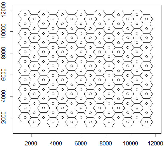
Figure 1.
Illustrative HEXIZON from main manual.
Figure 2 shows the pathway from inception to instantiation for a HEXIZON.
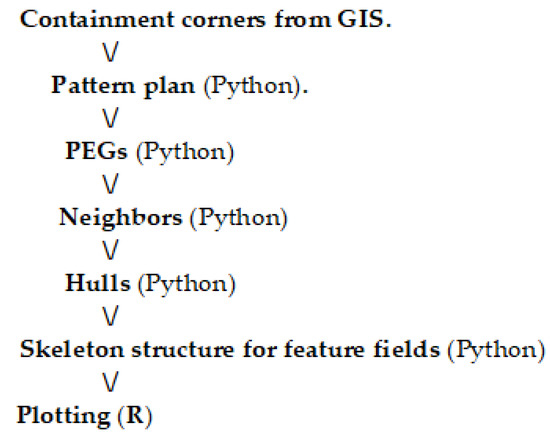
Figure 2.
Scripting scenario for HEXIZON.
In addition to the spatial structure shown in Figure 1, there is a tabular component to a HEXIZON that stores implicit indexing and feature fields. This is shown as the last part of the Python progression in Figure 2. The entire Python progression of Figure 2 can be refactored as a single script, but remains as a script of scripts for present purposes.
The containment corners of the HEXIZON at its upper-left and lower-right are read with the cursor of a desktop display in a GIS or interactive image analysis. The diagram of Figure 3 is basic to beginning a pattern plan.
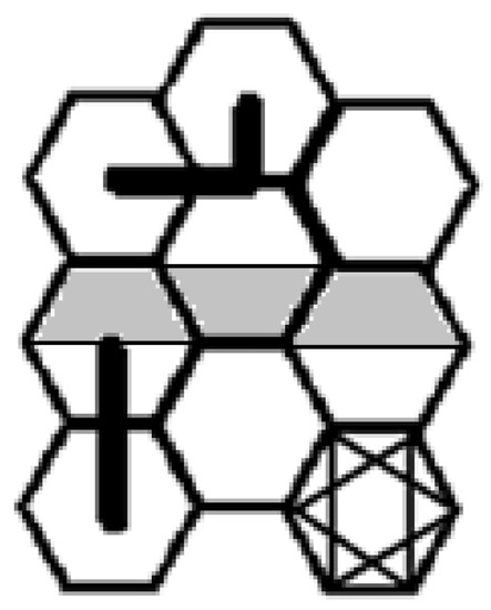
Figure 3.
Structure and spacing of hexagonal hulls.
The hexagonal hulls of Figure 3 are in columnar “canonical” configuration. A hull has a suite of structural elements such as length of side, height, and radial spoke from center to corner. The lower right hexagon of Figure 3 has an inscribed hexagram star. The span between opposing points of the star is one of the structural elements of the hexagon, and half of this span is the radial spoke from the center (hub) to a corner of the hexagon. The length of a line composing the star is the height of the hexagon in the columnar configuration. Half the height is the size of a spike from the center perpendicular to a side. Both the spoke and spike are central constructs for a HEXIZON. The spokes to either end of a side form an equilateral triangle, so the sides have the same length as spokes. As the boldest lines in Figure 3 show, the spacing between adjacent centers (hubs) in a column is a double spike; and there is (spoke + “halfspoke”) spacing between center-poles of the connected columns. The upper edge of the configuration has “humps and slumps”. The pattern plan must specify whether the HEXIZON begins with a slump or a hump.
Implicit indexing is a major motivation for having a HEXIZON as in Figure 4 since locations and adjacency aspects can be computed as adjusted integers, given coordinates of containment corners.
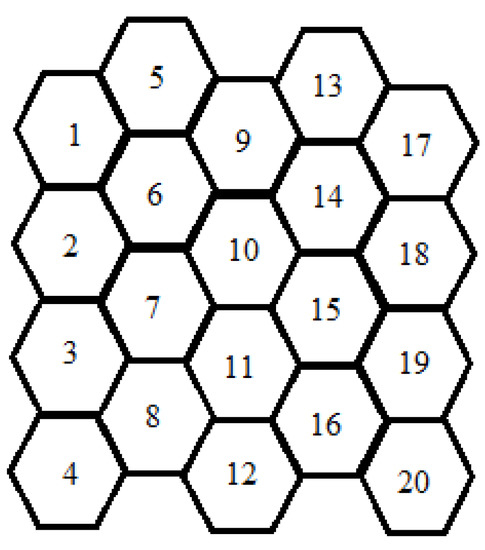
Figure 4.
Implicit indexing by columnar counting.
Perimeter progressions for hulls have characteristic configurations of connectivity. Perimeter progressions around hexagons form “rippled rings” with successive sequences having six segments more than the one before (Figure 4). These give recursive regimes for determining distance decay in regionalization of ratings.
2.1. Compiling and Collecting Content
Having constructed a HEXIZON framework, the next concern is content for feature fields. The pattern of PEG points is intended as a TAPON (Transferable Attribution Points Organizing Networks) poly-point portal into general geographic information systems (GIS). There is little difference in this regard from transferring waypoints from GPS (Global Positioning Systems). Each GIS software system, whether commercial or shareware, has its ways of importing spatial elements into its structure; but they have in common that point features are usually more readily accommodated than linear or areal features. They also have in common that most provide “buffering” capabilities, at least for point features. This suggests that interfacing with GIS by an export/import progression for pertinent PEG points [4].
Given that the GIS can import and buffer points, we need margin markers for circular buffer zones that will speak to a hexagonal context. “Spokes” and “spikes” are the appropriate margin markers. Spokes give circumscribed circles for hexagons, whereas spikes give inscribed circles. There is merit in having both buffers. The mean (or median) of the values for the two circular buffers should give an excellent surrogate for the hexagonal area itself, and the difference between the two buffers gives a marginal measure of sensitivity to scaling. Figure 5 shows a probable pathway for obtaining content from a GIS.
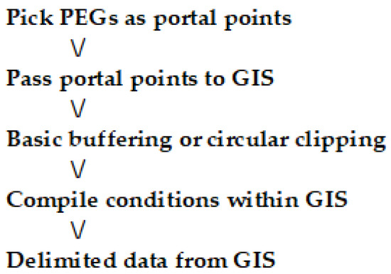
Figure 5.
Probable pathway for capturing content from GIS.
2.2. Proximal Propensity and Raised Regions
Having used Pythonic “HEXIZATION” to configure a HEXIZON, one can turn to analytical aspects for which R software is substantially superior. The HEXIZON can be analytically assimilated into R via its “read.table” facility for instantiating “data.frame” spreadsheets. Computational customization in R is accomplished as “function” facilities with versatile vectorization.
Regionalization of ratings can be considered in terms of exceedance through a rank-based regime called ROLS (Ratings of Less Strength). This is the exceedance that each individual hub/hull element has relative to other individual elements in the scope under surveillance (SUS). Exceedance is ordinal and countably quantitative. The minimum value of ROLS is always zero, and the maximum that it can have is one less than the number of elements in the SUS (normalized as needed). Thus, all elements have quantitative comparability for vicinity order relations (VOR). Cumulating such counts over immediate neighbors provides a Local Ordinal Cumulative Indicator (LOCI) for concentration of exceedance in a focal neighborhood.
A full “rippled ring” of nearest neighbors has six PEG positions. Each extra (entirely) encompassing rippled ring has six PEGs more than the one before. Ring relations are like “lags” in general geostatistics [10]. Peripheral progressions process PEG Index Number (PIN) pointers in list logistics, systematically screening prospective positions for new neighbors of neighbors while counting candidates and pushing process pointers. Implicit integer indexing is an essential enablement for vectorized versions of locational list processing procedures in R scripting strategies.
A custom component of the shared scripting strategy is an R function facility offering output options of VOR vectors that can constitute feature fields. The output options are ROLS, LOCI, and VOCI (Vicinity Ordinal Cumulative Indicator), with VOCI cumulative over a two-ring region around each element. Successive subtraction gives respective rings: LOCI–ROLS or VOCI–LOCI. Plotting LOCI against ROLS shows raised-ring regions and plotting VOCI against LOCI shows peripheral persistence of raised or rarified rating. Figure 6 shows a scripting scenario for probing proximal propensity and raised regions.
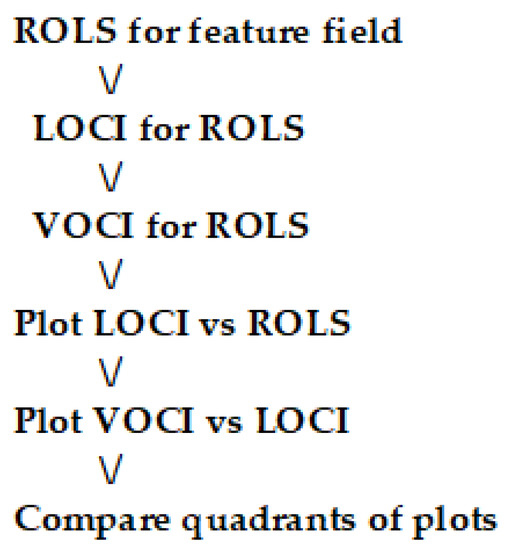
Figure 6.
Pathway for proximal propensity and raised regions.
2.3. Compound Connectivity and Hyper-Hills of Intensified Indicators
Varying values on a status scale can constitute a virtual vertical topographic topology of humpy hills and varied valleys. Slicing such scales into strata is standard strategy for showing summits and shallows of intensified interest in GIS. Such strata are cross-cutting, not naturally site specific. Extended exploration of strategic surveillance for site specificity targets topology trees [11] from tips through successive stems. Topology trees carry compound complexity, and shared scripting seeks to segregate salient structures.
Hyper-hills are hills on hills on hills in a rising recursion. Hyper-hill hypotheses concern surficial step structure, with a null hypothesis as a randomized region. Common contagion has several sizes and shapes of hills with scatterings of smaller sidehills and “climbing components” as pads of perched peaks. A hyper-hills hypothesis is subject to truncation testing that crops capping components.
Compound connectivity is a crucial computational concern for finding formations of (virtual) vertical variation. Sectors of sameness as contiguous conditions must be comprehensively compiled. Faux feature fields can store sector structures as linked lists that comprise a fusion field. The sheath of a sector contains contrasting contacts as edging elements. A sector sheath catalogues conditions contacting the sector. A sector sheath cannot be contained in a faux field since a single element can be in more than one sheath. Internally indexed vectors are versatile vehicles for staging sheaths. Prior preparation of particulars such as sectors in sheaths contribute to computational convenience.
Virtual verticality of both singles and sectors entails edge expression, which can be projection, progression, or depression. Projections are above every edging element. A progression has edge elements above and below. Depressions are below every edging element. Hyper-hills have projections as their peaks (or plateaus) in primary position. A projection is protracted when/where there is subsidence or stasis on all sides. When subsidence or stasis meets an external rising reversal, then protraction stops at the level of the rise with the protracted progression being perched. A perch progression is plotted and used for topological truncation. Plotting truncated topologies speaks to a hyper-hill hypothesis which can be supported by logical leveling for pruned projections. Figure 7 is an abbreviated analytical agenda for TIP and STEM topology; where TIP is for Terminal Insular Projections and STEM is for Saddle Truncated Elevated Mergers.
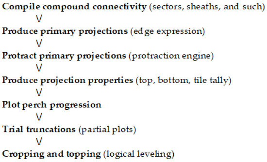
Figure 7.
Abbreviated analytical agenda for TIP and STEM topology.
2.4. Impaneled Indicators and Rating Relations
Surveillance seeks rating regimes of synthetic and surrogate signals summarizing system status. Interacting indicant items are intentionally impaneled, in computational contrast to data discovery. Restricted relative redundancy can contribute to consistency checking and commonality. Different density determinations can capture contextual considerations (such as road density or stream density). Strategy for synthesis seeks to segregate subsets for operational oversight.
Cross-coupled combinations of ROLS ratings are convenient comparative companions for clustering [12] and treatment of ties. Partial panels as data domains help to reduce redundancy and decrease dimensionality. Site specific concordance or conflict of components provides perspectives for prioritization of PEG positions in collective context. Definite discrepancies involving impaneled indicators are detectors of potentially problematic progressions (Hexagonally Impaneled Detector Networks). Figure 8 is an adaptable agenda for initial investigation with impaneled indicators in R.
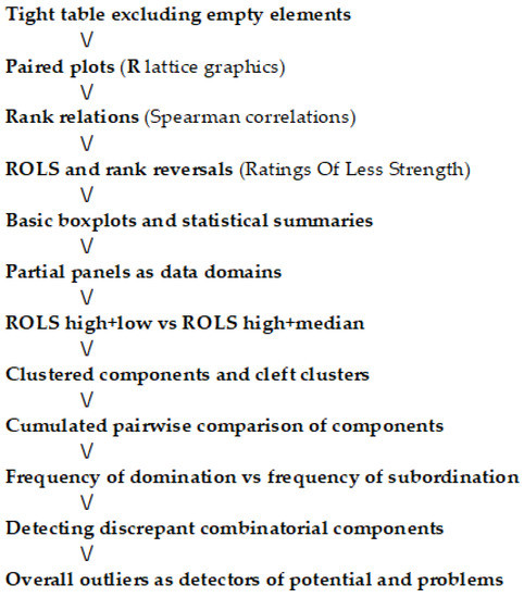
Figure 8.
Adaptable agenda for impaneled indicators.
3. Representative Results
Data regarding a collaborative conservation context that originated with The Nature Conservancy were used by Myers and Patil [13] as a subject for analytical approaches in R. The data are thereby well documented in conjunction with R computation and publicly available in the “Gap Analysis” reporting [14]. With some modifications, that context is carried forward to comparative conclusions after appropriate alterations of analytical agendas in foregoing figures and adding extended explanations to increase insight. The sequel setting entails a subset of a continental hexagonal tessellation. The subset lies in Pennsylvania, USA. The hexagonal tessellation by The Nature Conservancy was configured on a geographical coordinate referencing system (CRS) with the hexagons in slanting sequences that are not in collinear orthogonal order (i.e., not axially oriented). Each hexagonal tile covers 365 square km (11.055 km on a side) and carries a numeric identifier with identifiers running along a slanting sequence. The feature fields for the subset were segregated in a simply structured (space delimited) textual file. Illustrations and tabulations are drawn directly from R output.
A rigid rotation (with optional translation) is needed to achieve axial orientation for implicit indexing of location. A simple solution of local axes is chosen here that gives integer containment corners with a numerically neat range that accommodates an array of 11 columns (stacks of segments) having 17 hexagonal segments per column. The two containment corners for current computations with units in kilometers are as follows:
Upper left (X = 100, Y = 500); Lower left (X = 100, Y = 160); Upper right (X = 295, Y = 500); Lower right (X = 295, Y = 160).
Hexagons herein have margins matching the originals in Pennsylvania placement. Upward on Y is easterly, and upward on X is southerly. However, the last three hexagons in the last (11th) column are not part of the data domain for the state (empty elements). The hexagon identifiers are used to link (hexagonal) tiles to their original axial configuration. Figure 9 shows hexagon identifiers plotted in PEG positions using R graphics with negative numbers indicating empty elements. Original sequences of the identifiers run diagonally downward from the left in this figure.
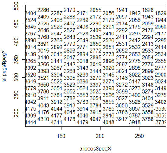
Figure 9.
Hexagon identifiers plotted in PEG positions.
The pattern plan as _hip.txt (hexagonal implicit pattern) file from a Python program is listed in Table 1.

Table 1.
Pennsylvania pattern plan as a _hip.txt file (R output).
First line of the pattern plan specifies 184 as region number and coordinates of one containment corner. Second line specifies 11 columns (first one shifted down) and the coordinates of the other containment corner. Third line specifies 17 PEGs per column with hexagons having maximum corner-to-corner (double spoke) of 22.11 km and hexagon height (double spike) as 19.14726 km. Fourth line signals lack of a metadata protocol followed by 16.5825 km as distance between center-poles of columns and then one-twelfth of a hexagon area.
PEGs are coded with integrative indicators and vicinity values as feature fields in data attribute tables, making PEG properties the counterpart of tile tables in tessellations. In the current conservation context, terrain tables provide PEG properties as shown by the first few lines in Table 2.
Table 2.
Top few lines of PEG properties showing indexing items and terrain data (R output).
The first line of Table 2 has headers. The second is a “leading line” of structural specifications. The third line is the first of the lines for positional properties with the hexagon ID number at the left. The next three fields contain implicit indexing information. There are six feature fields of terrain data. The “Birds” field is number of breeding bird species. The “Mamls” field is number of resident mammal species. The “ElvSD” field contains an indicator of elevation variability. The “PctFC” field is percent forest cover (at 100-hectare resolution). The “PctFP” field is percent of hexagon in one contiguous patch of forest cover (at 100-hectare resolution). The “PctOP” field is percent of hexagon in one contiguous patch lacking forest cover (at 100-hectare resolution).
3.1. Spatial Structures: Virtual Vertices, Singletons, Sectors, Sheaths, and Sites
Adjacency analysis is obligatory for obtaining truncated trends of topology. As previewed previously, a suite of R functions implicitly indexes aspects of adjacency for hinging hexagon hulls having virtual vertices. A “zone” consists of elements with common coding in a feature field. Sectors, as secondary structures, confer connectivity and continuity: similar to patches and paths of pavers. A sector is a contiguously connected component of a feature field as a specific same-status (sub)set with two or more cells. Thus, sectors and singletons comprise a feature field. This secondary structure can be recorded in either (or both) of two ways. One is “fusion field” as a “faux field” of PEG pointer properties containing linked lists for sectors. The other is as a “vector” version of “locator lists” specifying members of sectors by integer index PIN (PEG index number).
Whereas singletons have shared-side surrounds as neighbors by reference with a maximum of six, sectors have shared sides as a surrounding sheath with no fixed maximum length. Since sectors involve embedded elements and varying sizes, regular reference does not determine the sheath, which is obtained by adjacency analysis as an index vector of locator lists for sheath segments (lists of lists). An index vector of locator lists starts with an index to the list indexing. Each located list thus becomes a sort of super segment, and the computational context becomes one of list processing. Adaptiveness in algorithms leads to compound lists of lists comprising both sectors and singletons, with each such complex effectively creating a super segment. Sector sheathing cannot be cast as a faux field since a cell can occur in the sheaths of several sectors. It is only when each cell has a unique membership that a faux field can be formulated.
Compound collectives (structured sites) can be catalogued as a COSM (collectively organized site mosaics) that also uses implicit indexing of spatial structure. A COSM can be conserved as a simple serial file of delimited textual items. Virtual vertices of a hexagonal hull (also called “portico points”) can be instantiated immediately as proximate positions of a particular PEG, thus affirming that PEGs are primary positions and also operative objects for object-oriented programming.
3.2. Spatial Structures: Truncated Trends of Topology
With implicitly located lists allowing sectors and super sectors to be treated as singulars, it becomes tractable to explore tessellated topologies in multiple modalities such as “protracted projections” and “saddle sequences” as an outgrowth of earlier work in “echelons” [11,15,16]. This is tactical topology to locate increased intensity of an ordinal or interval indicator in an objective manner.
A topology “projection” is considered here to be a singleton or sector having all neighbors with lesser values of the indicator in question. A “protracted projection” is a contiguous set of cells for which all nonmember neighboring elements (singleton or sector) have lesser values of the indicator than any member and at least one such nonmember neighboring element has a nonmember neighbor in the range of or exceeding member elements. Then such a nonmember neighbor is a constituent of a “saddle”. A protracted projection is thus a contiguous capping structure or “hillock” perhaps perched on a larger “hill” of humpy hills and varied valleys.
Focusing on bird species richness, the process begins with assembly of an indexed projection vector (ipv) that appears as follows:
Birdipv
[1] 0 20 10 16 31 37 52 63 67 72 74 87 93 95 100 105 125 144 149
[20] 169 172 175
The first element of this vector is number of projecting sectors (none) and the second element is number of projecting singletons (20). Lacking any projecting sectors, the remaining elements are implicit index numbers of hexagons that constitute projecting singletons. If there were projecting sectors, a subindex to these would begin in the third element. A key aspect of such index vectors is that implicit indexing allows all elements of the vector to be integers. An R vector requires all elements to be of the same nature but is otherwise very mutable to the degree that this is a vector of indices to lists along with the lists themselves. Vectors are not fixed in R.
Conversion is then made to a COSM (collectively ordered site mosaics) demarcated multilist ordered by decreasing indicator value for input to the protraction engine. Since the protracted projections are mutually exclusive, they can be conveyed either as a COSM or a faux field; but the faux field format is used for plotting the protracted projections as in Figure 10.
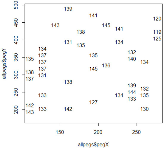
Figure 10.
Bird species richness values for protracted projections.
It is emphasized that protracted projections as plotted in Figure 10 are raised regions of the rating relief relative to their surroundings, some of which are “perched” higher up and others “perched” lower down. Primary peaks and subsidiary peaks will be found among them, along with hillocks on hills and humps in hollows. Those that are “low and shallow” can have all their indicator (rating) values less than some of the values not having membership in any of these projections—such as subordinate sections of hillforms. Therefore, it is essential to have further information about these formations.
The order of membership lists in the COSM version goes top–down according to decreasing local maximum as follows with zeros as delimiters of the membership lists and membership as implicit indices for hexagonal tiles.
Birdstps
[1] 95 111 0 105 123 0 149 148 167 133 150 166 0 16 15 33 0 37 0
[20] 67 0 87 0 144 162 143 0 52 0 10 11 27 25 26 8 24 28 0
[39] 63 0 72 0 74 57 0 93 0 125 0 31 0 169 0 100 0 175 174
[58] 0 172 0
The global maximum (145) occurs in two protracted projections each having two tiles. The next lower protracted projection is more expansive, consisting of six tiles. A table of projection properties (Table 3) provides information on “perch progressions” serving as surrogates for topological saddle sequences.
Table 3.
Properties of protracted projections (upper, bottom, tiles) as R output.
It is important to understand Table 3 thoroughly, since it is key to the topology of the indicator. The “site” column provides an identification number for each protracted progression, with sites listed in decreasing order of top height. Thus, lower numbered sites are more prominent features (except for ties). The “upr” (upper) column gives top height and the “btm” (bottom) column gives base height (with both having only ordinal metrication). “Perch” is used here as an alternate term for base to help prompt visualization. Where there is little difference between upper and bottom, the projection is “shallow”, with large differences being “deep”. A shallow projection with a high perch is still (part of) a prominent feature. A deep projection with a low perch “rises” out of a low-lying area to a substantial height, also needing attention. Within this context, the progression of perches is particularly important. A “humpy hill” will have small steps, whereas large drops show uninterrupted descent from “upland” to “lowland”.
Perch progression is obtained by sorting bottoms (btm) into decreasing order and then plotting as in Figure 11, which shows a gradual decline in perch position by one or two species from 143 to 130, and then definite drops. Thus, the upper-level structure is quite coherent with small shifts; then occurrence of transition to lower values with 130 being a transition threshold.
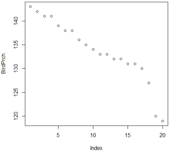
Figure 11.
Perch progression for protracted projections of bird species.
The “tls” column of Table 3 gives a count of tiling elements in the projection, showing whether the projection is expansive or localized; but not showing whether one part of the extent is “steeper” than another.
Figure 12 shows spatial structure of components above the perch progression threshold of 130. Figure 11 and Figure 12 exhibit characteristics of common contagion in regard to a hyper-hills hypothesis. Consider connectivity of compound capping components in the context of corridors [2,3,16].
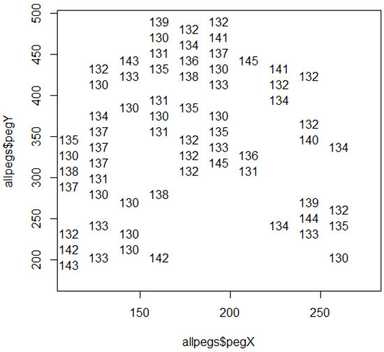
Figure 12.
Bird species richness above a 130 threshold for perch progression.
3.3. Spatial Structure: Rippled Rings of Relative Ratings
Indicators are ordinal (ordered) but not necessarily additive; however, ordinality implies exceedance and exceedances are countably quantitative. Ordinality supports ranking, with ratings of less strength (ROLS) or ranks of less strength being countably quantitative as exceedances. Therefore, ROLS constitute synthetic subordinate substrate for an instance of an indicator; and the numbers of exceedances among a set of instances are cumulatively countable as aggregate amounts. Therefore, ROLS signify substrate of a topology terrain. ROLS for related ratings defined over the same set of segments also become consistently comparable with respect to ordinality. The “head” (first few lines) of a subset of columns in the terrain table is shown as Table 4 after conversion to ROLS. Unlike regular ranks, ROLs values are integers since they are counts.
Table 4.
Head of a subset of columns from terrain table after conversion to ROLS (as R output).
The snippet in Table 4 shows that Birds may have substantial disparity relative to other indicators.
The ability to cumulate counts of exceedance as a pseudo-substrat provides a pathway for approaching aspects of radial regionalization involving indicators. Since indicators generally do not conform to the intrinsic hypothesis of geostatistics, patterns of spatial autocorrelation are seldom subject to methodic modeling but are nevertheless of inherent interest for empirical exploration. Each (interior) tile is encompassed by a “ring” of six neighbors that are implicitly indexed. That ring is encompassed by another ring of twelve tiles, etc., with (full) rings recursively expanding by six additional tiles. The cumulated content of a ring can be obtained by cumulating the content of the ring and its core, then subtracting the cumulated contents of the core. A progressive process works by cumulating neighbors with neighbors of neighbors (while checking to avoid duplication), then subtracting the corresponding core. If there is substantial autocorrelation, the cumulated contents for rings should show relations with cumulated contents for cores. The shift from ring to ring is like a lag in geostatistics. A simple such scenario is to plot BirdRing1 as ordinate against BirdROLS as abscissa in Figure 13. Spatial autocorrelation is evident in Figure 13, but there is substantial variation in the degree to which it is expressed, with notable outliers, particularly on the low side (some of which is due to edges). Each plotted point could be individually identified using the “identify” facility in R.
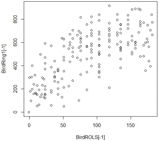
Figure 13.
BirdRing1 versus BirdROLS.
3.4. Regionalized Rating Relations: Impaneling Interrelated Indicators as Detector Networks
Encompassed exceedance or subordinate substrate computed as ranks of less strength (ROLS) provides for complex comparisons of spatial structure in an indicator that increases over an explicit encompassed extent (spatial scope). Such comparisons are conditional on selection of a specific scope. This constitutes intraset scaling as opposed to interset scaling. Such scaling is advantageous for investigation of impaneled indicators. Indicators are “impaneled” when deliberately designated for compound comparisons where complex concerns with collateral conditions call for coupling indicators to provide pertinent partial perspectives while contributing to commonality. This is unlike data mining or data discovery since indicators are intentionally included as opposed to opportunistically obtained. Definite discrepancies are detectors of discordance and possible problematic progressions.
A crucial concern is to screen for role reversal(s). In the current case there are three “flavors” of forest cover. One is percent forest cover for the hexagon (PctFC), a second is percent in largest contiguous cover (PctFP), and a third is percent in the largest contiguous nonforest patch (PctOP). Since the third increases in opposition to the other two, it is a counter-indicator. Such a counter-indicator is easily reconciled in rank ROLS by ranking in reverse (PctOPr).
3.5. Regionalized Rating Relations: Data Domains
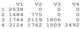
There is a second screening that looks for data domains as partial panels based on rank correlations. A data domain is a subset of indicators that are more closely interrelated than to other indicators. This panel has two data domains as given in Table 5, with the connections being (rank) correlations.
Table 5.
Data domains in terrain table of indicator ROLS (R output).
The ROLS are placed in two domains, with the first consisting of forest indicators led by PctFC and PctFP and the second having Mamls, ElevSD, and Birds led by Mamls and ElevSD. The leaders in the first domain are so closely linked that they could substantially serve as surrogates (redundant ratings). Therefore, it is appropriate to drop a redundant rating PctFP (% largest forest patch).
3.6. Regionalized Rating Relations: Cross-Coupled Combinations of ROLS Range Ratings
Impaneled indicators with ROLS ratings are consistent for cross-comparisons, but differences in diversities due to ties are collateral considerations. Adding the minimum and maximum across a panel or partial panel on a tile-by-tile basis makes a convenient composite. From a statistical perspective, this is double the midrange but preserves the integer nature of ROLS. It does not, however, convey any direct sense of the variability among the ROLS for the impaneled indicators. To capture some sense of the latter, a second summation is maximum plus median. It eliminates the effect of the lower half of the ROLS for impaneled indicators. When the maximum plus minimum is plotted as an ordinate against maximum plus median as an abscissa, the difference between the axes reflects the influence of the lower half of the ROLS values, as shown in Figure 14 for five impaneled indicators. Locations plotting in the upper-right corner are most consistently propitious across all indicators, and those plotting in the lower-left are least so. Locations of interest can be retrieved individually or through thresholds.
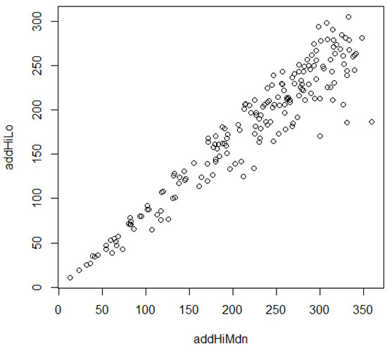
Figure 14.
High plus low ROLS on y-axis versus high plus median on x-axis.
3.7. Regionalized Rating Relations: Contextual Collectives
Composite combinatorial criteria such as those in Figure 14 have the advantage of retaining ordinality, but do not speak to particular permutations. Partitioning of patterns into contextual collectives [13] without combinatorial compensation comes from clustering via the R hclust() hierarchical clustering facility, which takes a distance matrix from the dist() facility as intermediary input. The level of (dis)aggregation is then specified via the cutree() command. This approach can be used to obtain nine numbered clusters with which to label the points of Figure 14 in producing Figure 15.
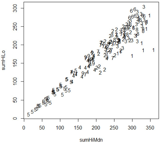
Figure 15.
High plus low vs. high plus median, labeled by cluster number.
Instances that appear close in Figure 14 but have different numbers in Figure 15 will show segregation in at least some of the indicators. Importantly, the numberings of the clusters in Figure 15 are essentially just labels. They do not serve to order the clusters in a comparative respect.
There are general patterns of placement for the clusters but also scatterings. Cluster 5 is low and cluster 6 is high. Clusters 3 and 8 are scattered in the upper limb. Cluster 1 is on the upper-right flank where some lower ROLS contrast with higher ones. Clusters 4 and 9 tend to be central. Clusters 2 and 7 are quite widely dispersed in the upper half. Twelve clusters allow for splitting one-third of the clusters, and cross-tabulation in Table 6 shows how splitting takes place.
Table 6.
Cross-tabulation of nine clusters (columns) vs. twelve clusters (rows) as R output.
Clusters 3, 5, and 7 are split (refined). Cluster 3 is extensively interspersed with others in Figure 15 where it includes even the upper-right corner element. Cluster 5 is considerably cohesive, but encompasses most of the lower-left corner along almost a third of the diagonal. Cluster 7 is extensively interspersed along the central third of the diagonal in Figure 15. Refinement of these three clusters is clearly appropriate, so the 12-cluster breakdown should replace the earlier 9-cluster version.
3.8. Regionalized Rating Relations: Panel Paired Primacy
The logic regarding subordinate substrate with intraset scaling as ROLS can be extended to (original) interset scaling with set-specific comparisons. Familiarity of scaling is thereby retained, and comparisons already conducted need not be redone when a set (scope) is expanded. This proceeds in terms of pairwise primacy. Primacy (or lack thereof) for a pair of (positional) elements takes one of four conformance conditions.
Compound comparison of case couplets is considered conformant when the component criteria (indicators) are consistent with respect to order. There are three conformant conditions. Two cellular cases are concordant if their indicators do not differ. A cellular case is dominant over a subordinate when none of the indicators are diminutive (less than) relative to their counterpart, and at least one of the indicators is greater than its counterpart.
If one case is neither dominant, concordant, nor subordinate relative to another, then the two cases are variant relative to each other. Collective comparison for a case relative to the others entails compiling the frequencies of dominant, concordant, and subordinate (dcs) conditions, with any residual being variant. A table of primacy properties thus has three columns with as many rows as there are cellular elements. An implicit column of (residual) variants completes the case counts for rows.
Consider this for four of the terrain table features: Birds, Mamls, ElevSD, and PctFC. Perspective is provided by plotting dominant frequency against subordinate frequency with a diagonal line to show the degree of indecision (conformant plus variant) [17] in Figure 16. The identified instances in Figure 16 are numbered one less than lines in the dataframe due to exclusion of a layout line. There are particularly poor elements in lines 172 and 159 of feature files.
@ hxIDtabl[172,]
seg col pin Birds Mamls ElevSD PctFC
1829 1 11 171 96 34 17 25.3
@ hxIDtabl[159,]
seg col pin Birds Mamls ElevSD PctFC
2294 5 10 158 103 39 15 11.9
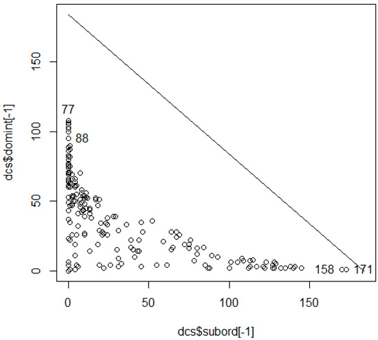
Figure 16.
Dominant versus subordinate from dcs tabulation for Birds, Mamls, ElevSD, and PctFC.
Likewise, a substantially superior group can be obtained as follows.
@ hxIDtabl[dcs$domint > 95,]
seg col pin Birds Mamls ElevSD PctFC
2647 4 3 38 133 48 135 95.7
2527 4 4 55 135 49 120 88.6
2648 5 4 56 129 52 126 98.5
2171 1 5 69 132 50 104 97.5
3143 9 5 77 132 50 118 91.0
3527 14 8 133 134 52 142 84.6
One can then proceed to probe which particular properties are prominent causes of contrary conditions leading to lack of conformance.
3.9. Regionalized Rating Relations: Detecting Discrepant Combinatorial Components
The foregoing focuses on conformant comparisons, but contrary comparisons are also informative. Nonconformant case comparisons have three separable situations. Firstly, there may be a single contrary indicator with the others being conformant. Secondly, there may be a plurality of conformant indicators with a minority of contrary ones. Thirdly, there may be equal numbers of conformant and contrary indicators. A function facility compiles these three types in a matrix. The diagonal discloses single contrary occurrences of each indicator. The upper triangle shows oppositional occurrences wherein the minority involves two or more indicators. The lower triangle shows oppositional occurrences of even splits. The resulting matrix follows.
Oppositional even splits can occur with an odd number of indicators when some of the indicators have the same value. With only four indicators, there is no possibility for a minority of two indicators—so the upper triangle of this matrix is empty.
The Birds (variable 1) and PctFC (variable 4) are more frequently individually nonconformant, and the Mamls (variable 2) indicator is least often a lone nonconformant. Birds conflict most often with PctFC reflecting grassland birds, wetland birds, etc. Mamls conflict most often with ElevSD (variable 3), since lowlands can support a diversity of mammals.
4. Discussion
The HEXIZON and procedural pathways in methodology are convenient constructs for conveying concepts, but may initially imply constraints on configurations and computations that are actually absent. R is a very versatile platform, as witness its extensive CRAN library of contributed capabilities including substantial spatial software along with ordinal operations. Recasting of routes to results and embedding extended explanations should have shown some of the scope for strategizing. HEXIZON is appropriate as a moniker for a rectangular scope under surveillance (SUS) containing a hexagonal pattern of posting points, since a feature field focused on the posting points is a zonation and the collective containing a common code is a zone without regard to connectivity. Provision is made for archiving a zonation that has integer coding in a compressed configuration as a delimited data file having a “_zon.txt” suffix on its name.
The novel nature of the HEXIZON construct is post patterning and dual design for what may be called commensal computing. In post patterning, posting points promulgate a pattern and are primary with respect to properties and proximities. This finds further featuring in the associated acronym TAPON. In dual design, each posting point is the hub for a hull that delimits its direct domain. A combination of hubs and hulls is a nucleated network with dual network architecture (DNA). With commensal computing, one system imposes on another system for a particular purpose without doing detriment. A nucleated network may have hinging hulls forming a tight tessellation. The vertices for hexagonal hinging hulls are portico points. Having hulls extend beyond hinging induces intricate interweave. A HEXIZON is commensal relative to GIS, whereas R is a companion relative to Python in this context.
Implicit integer indexing as PINs (positional index numbers) is critical for locational logic and computational capabilities in both R and Python. Accordingly, the HEXIZON has orthogonally oriented cross-collinearity of posting points as hubs for hexagons. The cross-column collinearity also includes pairs of portico points so that hexagonal hulls have horizontal tops and bottoms. This is structurally sufficient to provide PINs as implicit integer indices that only require simple single sequencing in “vectors” of variation. With implicit indexing, regionalization of ratings can be explored explicitly without conducting coordinate computations, thus, making truncated topology tractable as hyper-hills.
Ideas of implicit indexing can be extended to implicit informatics for facilitation of progressive prototyping and modularization as methods in object-oriented operations. A precursor plan sets the stage for cumulative constructs. The pattern plan is an initial inception of a HEXIZON that harbors sufficient specifications for subsequent staging of explicit establishment as the Python pathway in the prior presentation of methodology. An alternative arrangement for the Python pathway of programs is modular methods that are incrementally invoked in a structured scenario subject to stopping or starting at some selected stages. This is a priority in progressing from production prototype to packaging for practicality.
Static structure carries constraints. HEXIZON primary postings are insufficient for interpolative inquiry commonly conducted in generalized geostatistical settings that gave rise to representations of “regionalization” [10] in proximal propensity when given particular points of definite determinations in selective and/or subjective spacings. The selective and/or subjective spacing is accommodated by partible probes and reciprocally referenced poly-probes. The attribution and filing of features are essentially equivalent to post patterning, but everything is explicit in both locational logic and associative aspects. Integer identifiers are retained for logistics of list processing, but positioning of probes cannot be implicitly inferred. Shifts of stationing in scenarios is appropriate. Partible probes can serve as scaling spindles for detecting disturbances or conditions of concern at different distances (radial ranges) in GIS. Associations are ascribed as well as accessed by restricted referencing that can be reciprocal. Reciprocal sets require that each member be referenced by at least one other member, and necessitate searching for associates of all associates. A probe is purged by negating its number, rather than removal. A purged probe can be restored by negating the negation.
There are also partible peripheral posts along major margins of the scope under surveillance. Hexagonal hulls around PEG points leave hemi-hexagonal gaps along the upper and lower edges that can be filled by tapering trapezoids. Trapezoid Auxiliary Points (TAPs) are positioned on these margins and interpolation is available for filling features to level the lattice.
Having hexagonality of principal pattern provides possibility for refinement of resolution by situating secondaries such that they split sides of hinging hexagons with plan parameters adjusted accordingly. Secondary segmentation should be selective rather than synoptic, with subscopes of secondary structure. Subsidiary scopes interior to a HEXIZON are obtained as quadrangles specified as PINs of upper-left and lower-right margin markers for encompassed elements. Pursuit of this possibility would engender hyper-hexagonal HEXIZONs with underlays in the subsidiary spaces.
Funding
The Pennsylvania State University provides facilities support.
Institutional Review Board Statement
Not applicable.
Informed Consent Statement
Not applicable.
Data Availability Statement
Data are contained in an appendix to the software manuals.
Conflicts of Interest
The author declares no conflict of interest regarding content.
References
- Patil, G.; Myers, W.; Luo, Z.; Johnson, G.; Taillie, C. Multiscale assessment of landscapes and watersheds with synoptic multivariate spatial data in environmental and ecological statistics. Math. Comput. Model. 2000, 32, 257–272. [Google Scholar] [CrossRef]
- Hong, H.-J.; Kim, C.-K.; Lee, H.-W.; Lee, W.-K. Conservation, Restoration, and Sustainable Use of Biodiversity Based on Habitat Quality Monitoring: A Case Study on Jeju Island, South Korea (1989–2019). Land 2021, 10, 774. [Google Scholar] [CrossRef]
- Valeri, S.; Zavattero, L.; Capotorti, G. Ecological Connectivity in Agricultural Green Infrastructure: Suggested Criteria for Fine Scale Assessment and Planning. Land 2021, 10, 807. [Google Scholar] [CrossRef]
- Myers, W.L.; Patil, G.P. Statistical Geoinformatics for Human Environment Interface; Informa UK Limited: London, UK, 2012; ISBN 978-1-4200-8287-6. [Google Scholar]
- Brüggemann, R.; Patil, G.P. Ranking and Prioritization for Multi-Indicator Systems; Springer Science and Business Media LLC: Berlin/Heidelberg, Germany, 2011. [Google Scholar]
- Myers, W.; Patil, G.P. Biodiversity in the Age of Ecological Indicators. Acta Biotheor. 2006, 54, 119–123. [Google Scholar] [CrossRef] [PubMed]
- R Core Team. R: A Language and Environment for Statistical Computing; R Foundation for Statistical Computing: Vienna, Austria, 2019. [Google Scholar]
- McGrath, M. R for Data Analysis; Easy Steps Ltd.: Warwickshire, UK, 2018. [Google Scholar]
- McGrath, M. Python in Easy Steps; Easy Steps Ltd.: Warwickshire, UK, 2015. [Google Scholar]
- Webster, R.; Oliver, M.A. Geostatistics for Environmental Scientists, 2nd ed.; John Wiley & Sons Ltd.: Chichester, UK, 2007; ISBN 978-0-470-02858-2. [Google Scholar]
- Myers, W.; Patil, G.P.; Joly, K. Echelon approach to areas of concern in synoptic regional monitoring. Environ. Ecol. Stat. 1997, 4, 131–152. [Google Scholar] [CrossRef]
- Myers, W.L.; McKenney-Easterling, M.; Hychka, K.; Griscom, B.; Bishop, J.A.; Bayard, A.; Rocco, G.L.; Brooks, R.P.; Constantz, G.; Patil, G.P.; et al. Contextual clustering for configuring collaborative conservation of watersheds in the Mid-Atlantic Highlands. Environ. Ecol. Stat. 2006, 13, 391–407. [Google Scholar] [CrossRef]
- Myers, W.; Patil, G.P. Multivariate Methods of Representing Relations in R for Prioritization Purposes: Selective Scaling, Comparative Clustering, Collective Criteria and Sequenced Sets; Springer: New York, NY, USA, 2012; ISBN 978-1-4616-3121-3. [Google Scholar]
- Myers, W.; Bishop, J.; Brooks, R.; O’Connell, T.; Argent, D.; Storm, G.; Stauffer, J., Jr. The Pennsylvania GAP Analysis Final Report; The Pennsylvania State University: University Park, PA, USA, 2000. [Google Scholar]
- Myers, W.L.; Kurihara, K.; Patil, G.P.; Vraney, R. Finding upper-level sets in cellular surface data using echelons and saTScan. Environ. Ecol. Stat. 2006, 13, 379–390. [Google Scholar] [CrossRef]
- Smits, P.; Myers, W. Echelon approach to characterize and understand spatial structures of change in multitemporal remote sensing imagery. IEEE Trans. Geosci. Remote Sens. 2000, 38, 2299–2309. [Google Scholar] [CrossRef]
- Myers, W.; Patil, G. Preliminary prioritization based on partial order theory and R software for compositional complexes in landscape ecology, with applications to restoration, remediation, and enhancement. Environ. Ecol. Stat. 2010, 17, 411–436. [Google Scholar] [CrossRef]
Publisher’s Note: MDPI stays neutral with regard to jurisdictional claims in published maps and institutional affiliations. |
© 2021 by the author. Licensee MDPI, Basel, Switzerland. This article is an open access article distributed under the terms and conditions of the Creative Commons Attribution (CC BY) license (https://creativecommons.org/licenses/by/4.0/).