
Landscape Ecological Analysis of Green Network in Urban Area Using Circuit Theory and Least-Cost Path

Abstract
:1. Introduction
2. Methodology
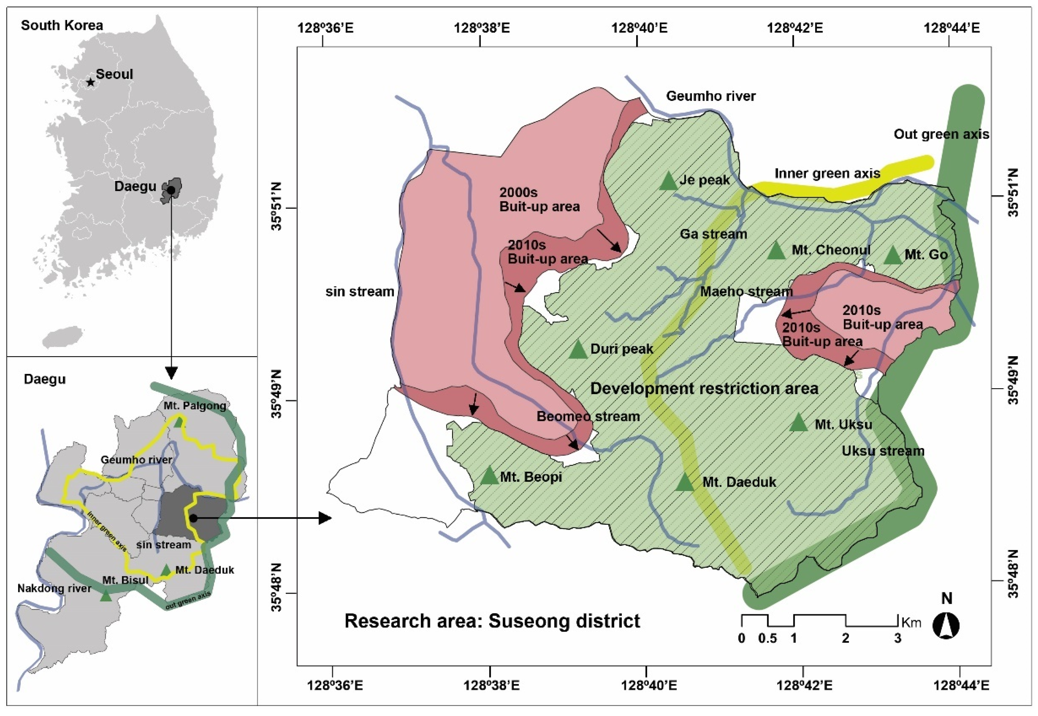
2.1. Research Area
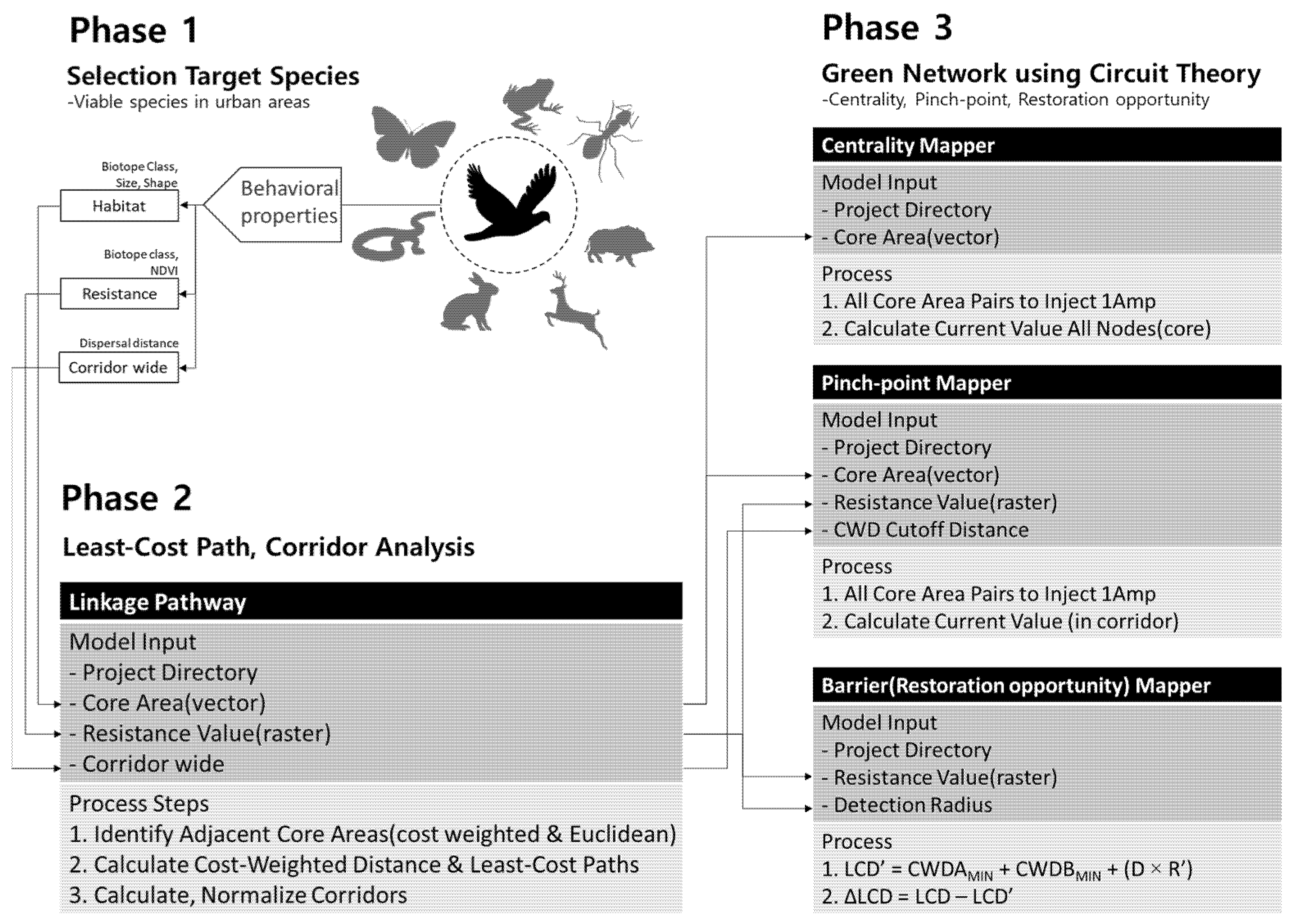
2.2. Research Framework
2.2.1. Selection of Target Species and Extraction of Core Green Areas
2.2.2. Least-Cost Path Analysis
2.2.3. Analysis of Green Network Using Circuit Theory
3. Results
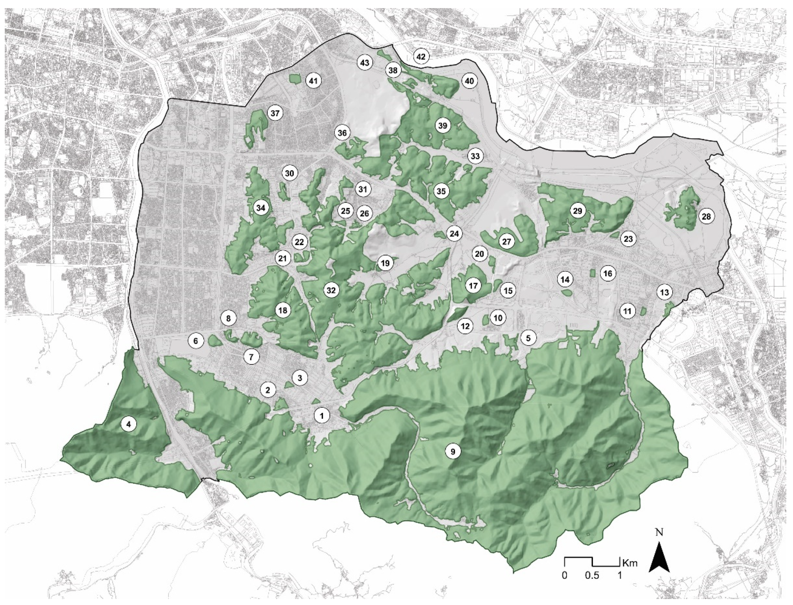
3.1. Core Green Area Extraction
3.2. Least-Cost Path Analysis
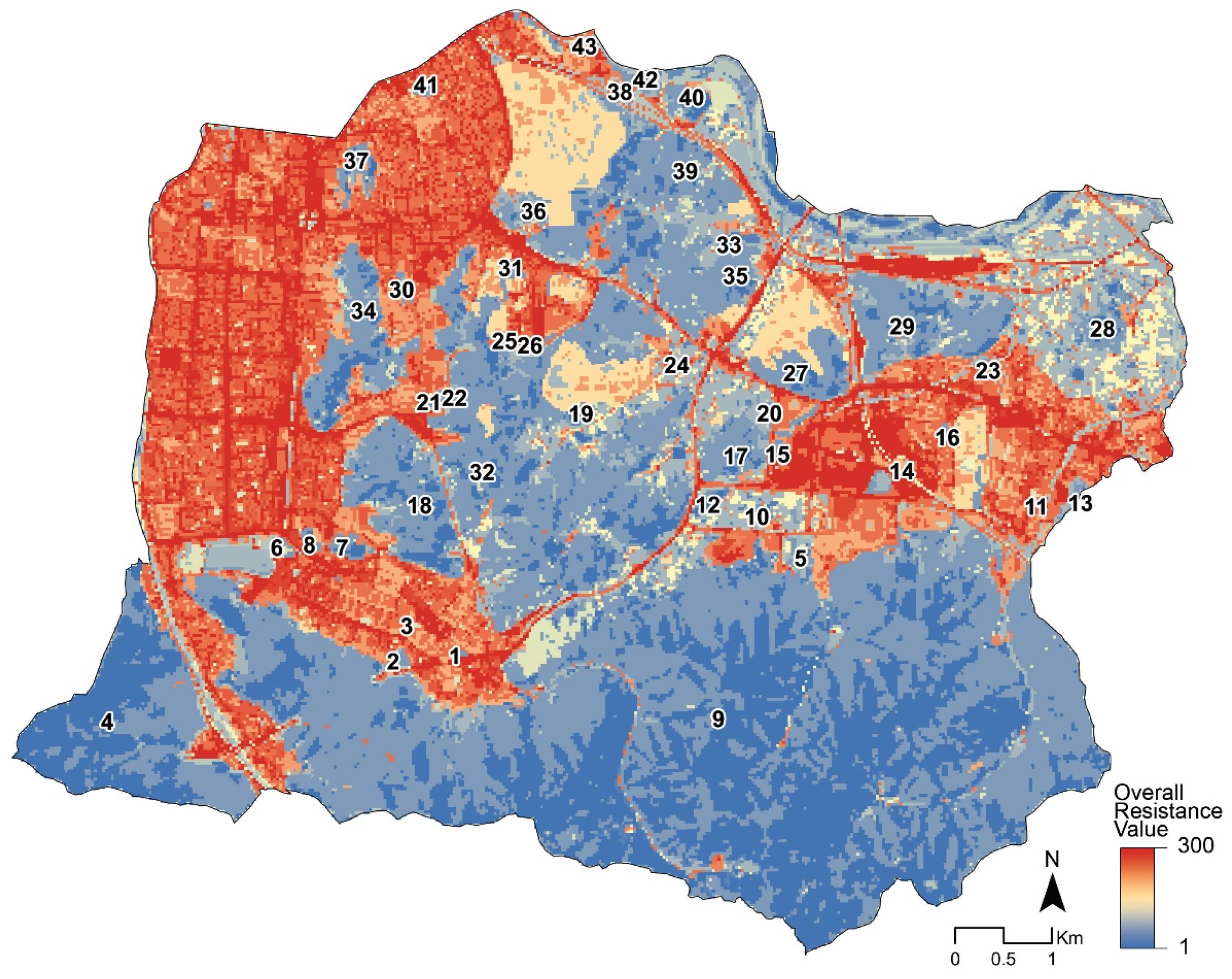
3.2.1. Resistance Value and Resistance Surface Calculation
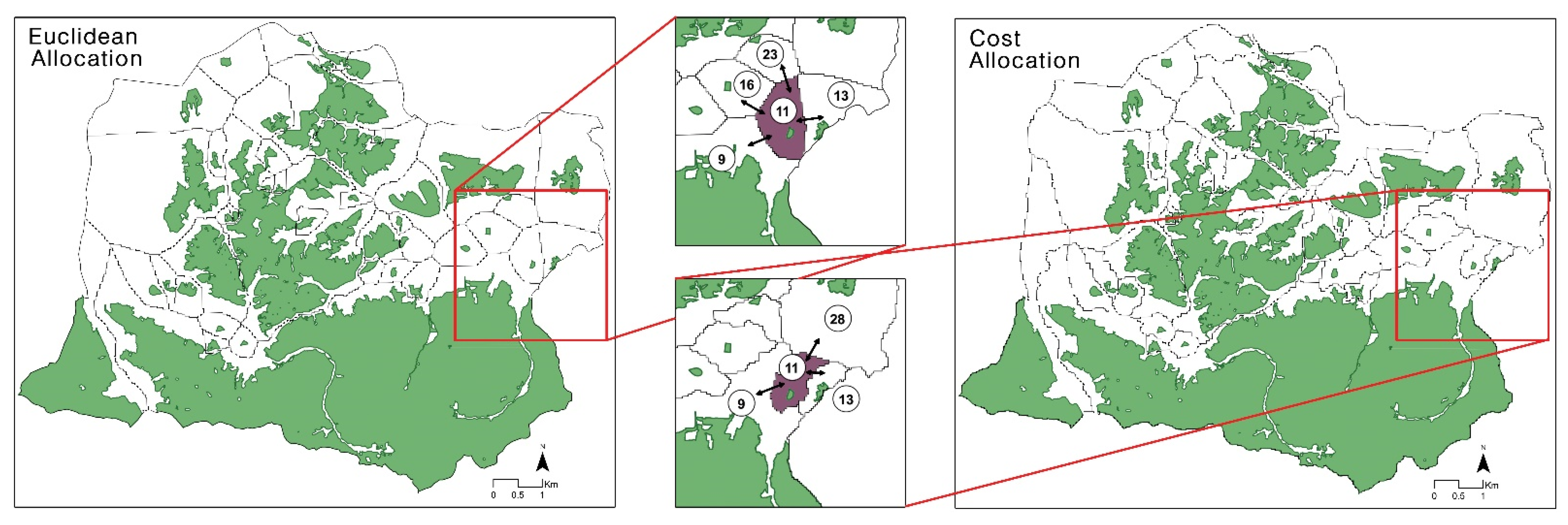
3.2.2. Result of Proximity Allocation Analysis between Core Green Areas
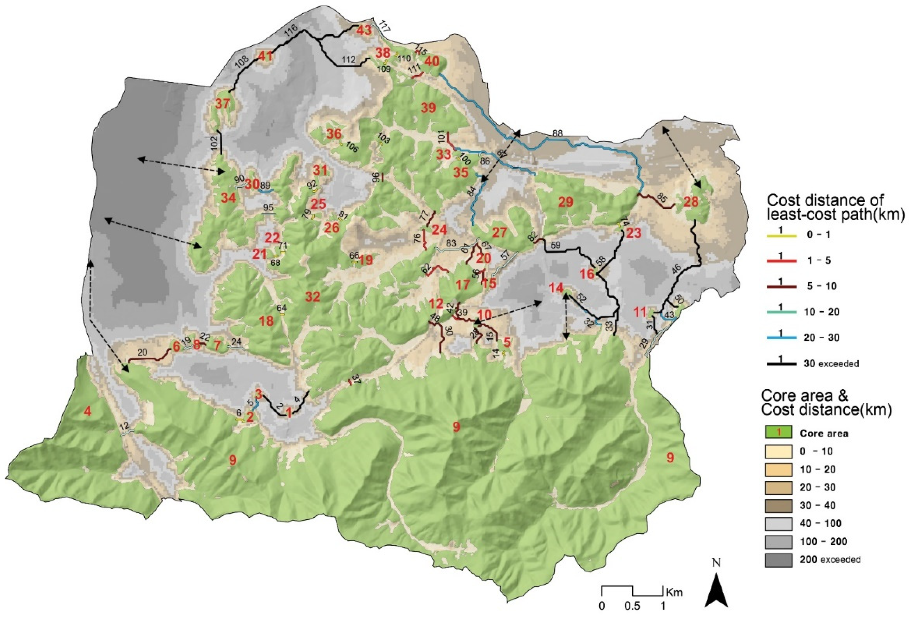
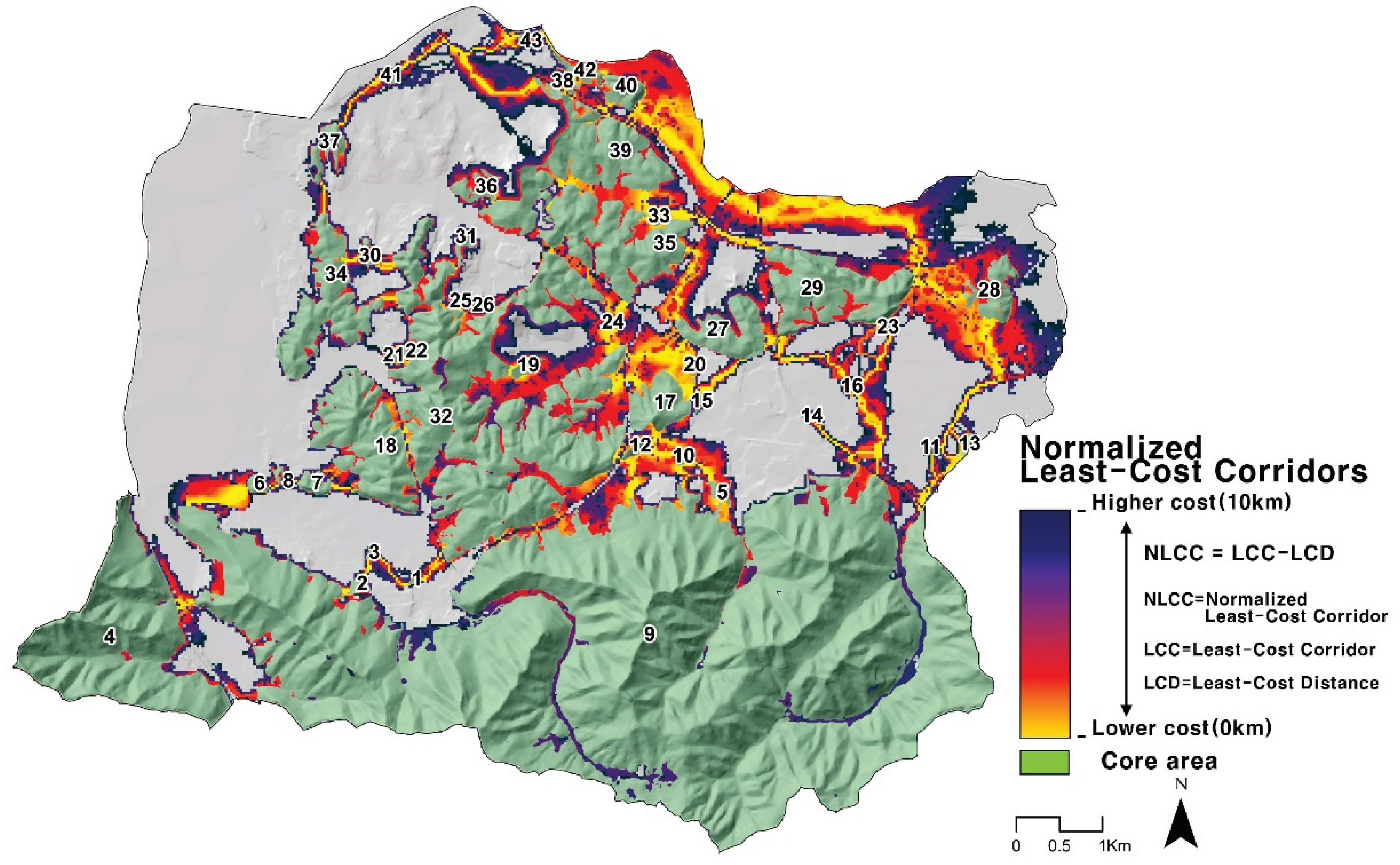
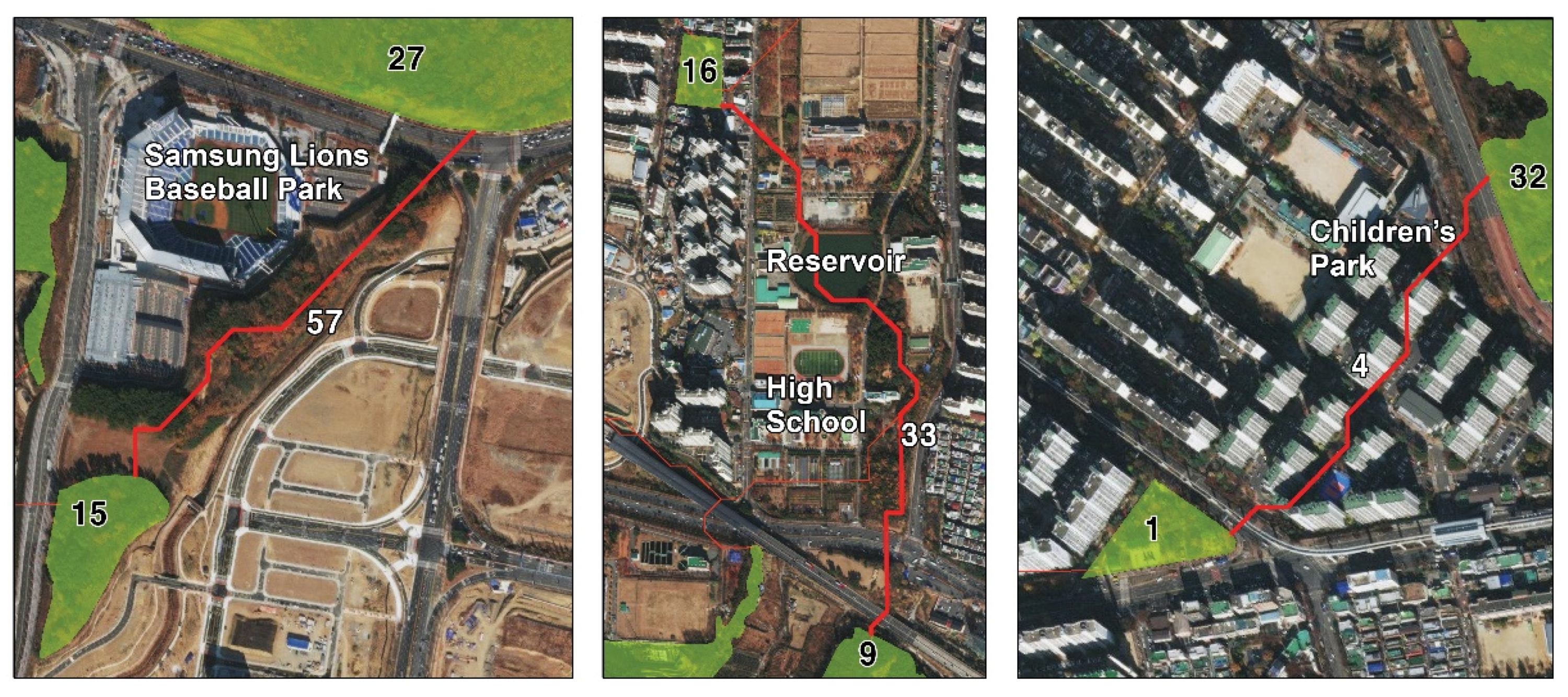
3.2.3. Least-Cost Distance, Least-Cost Path and Corridor Analysis Results
3.3. Centrality, Pinch-Point, Restoration Analysis
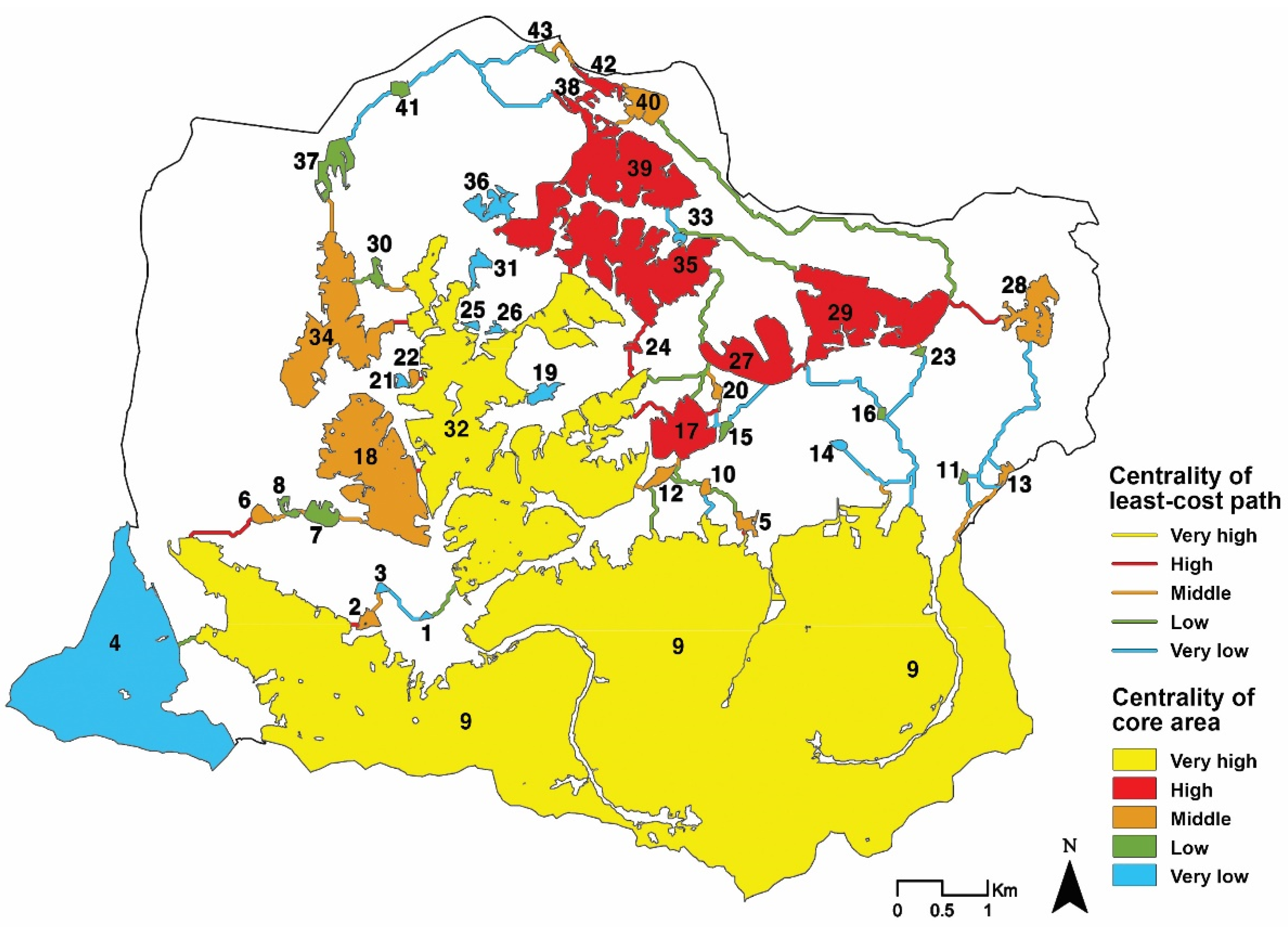
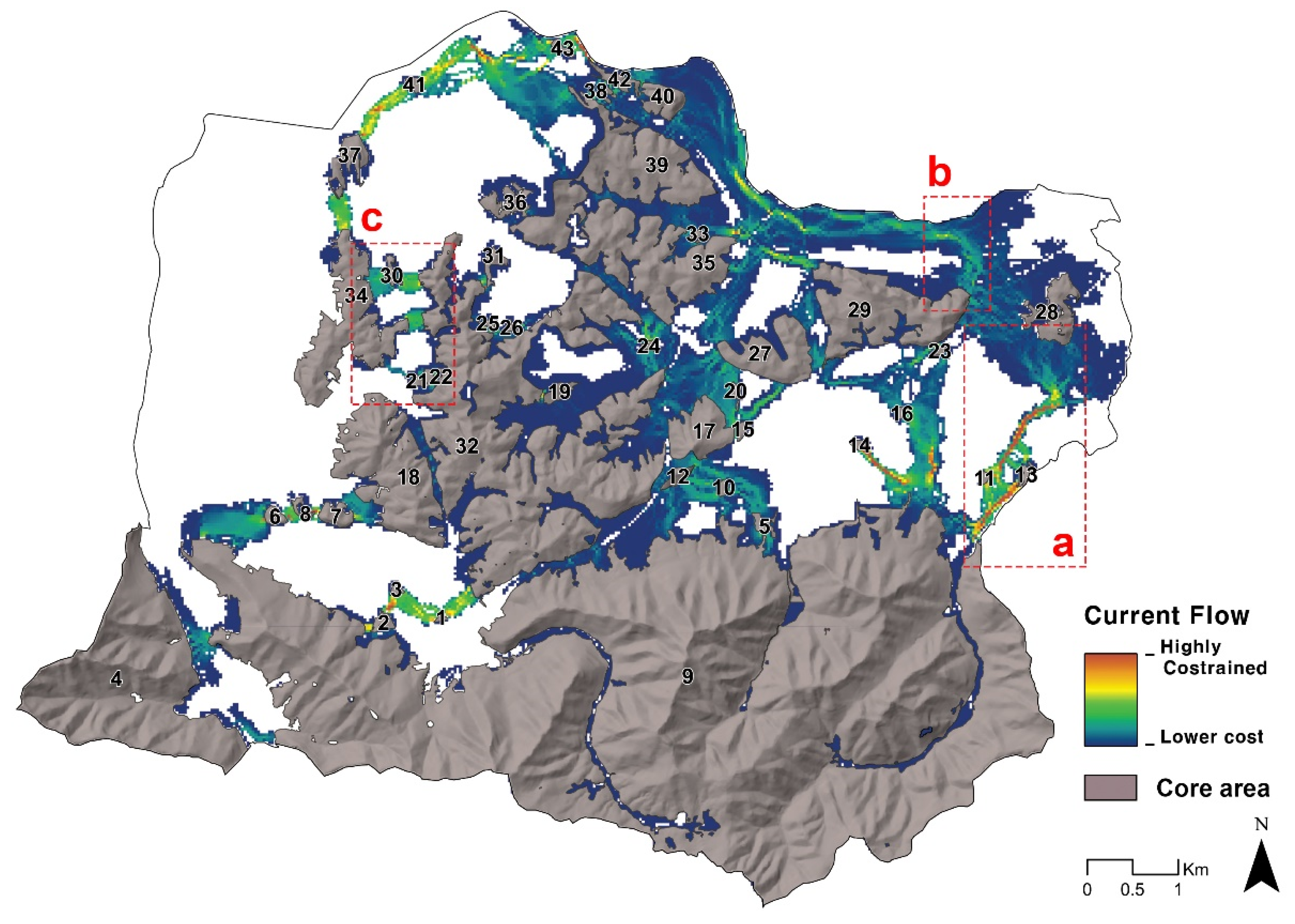
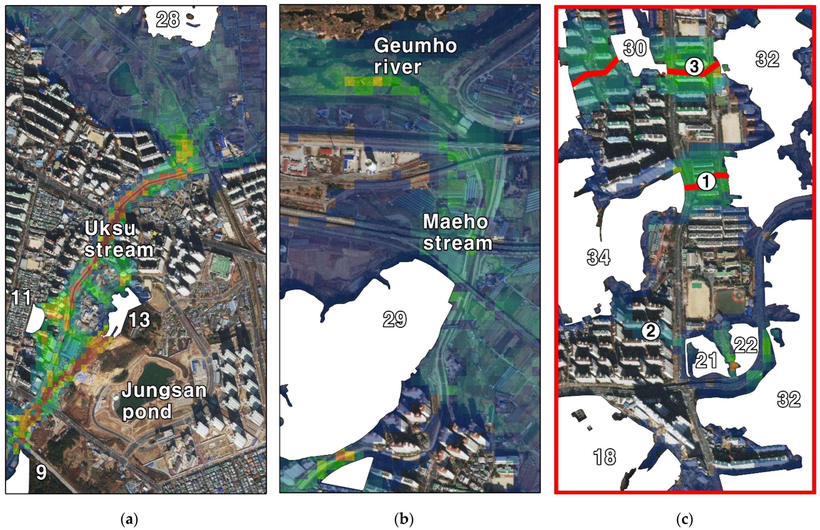
3.3.1. Centrality
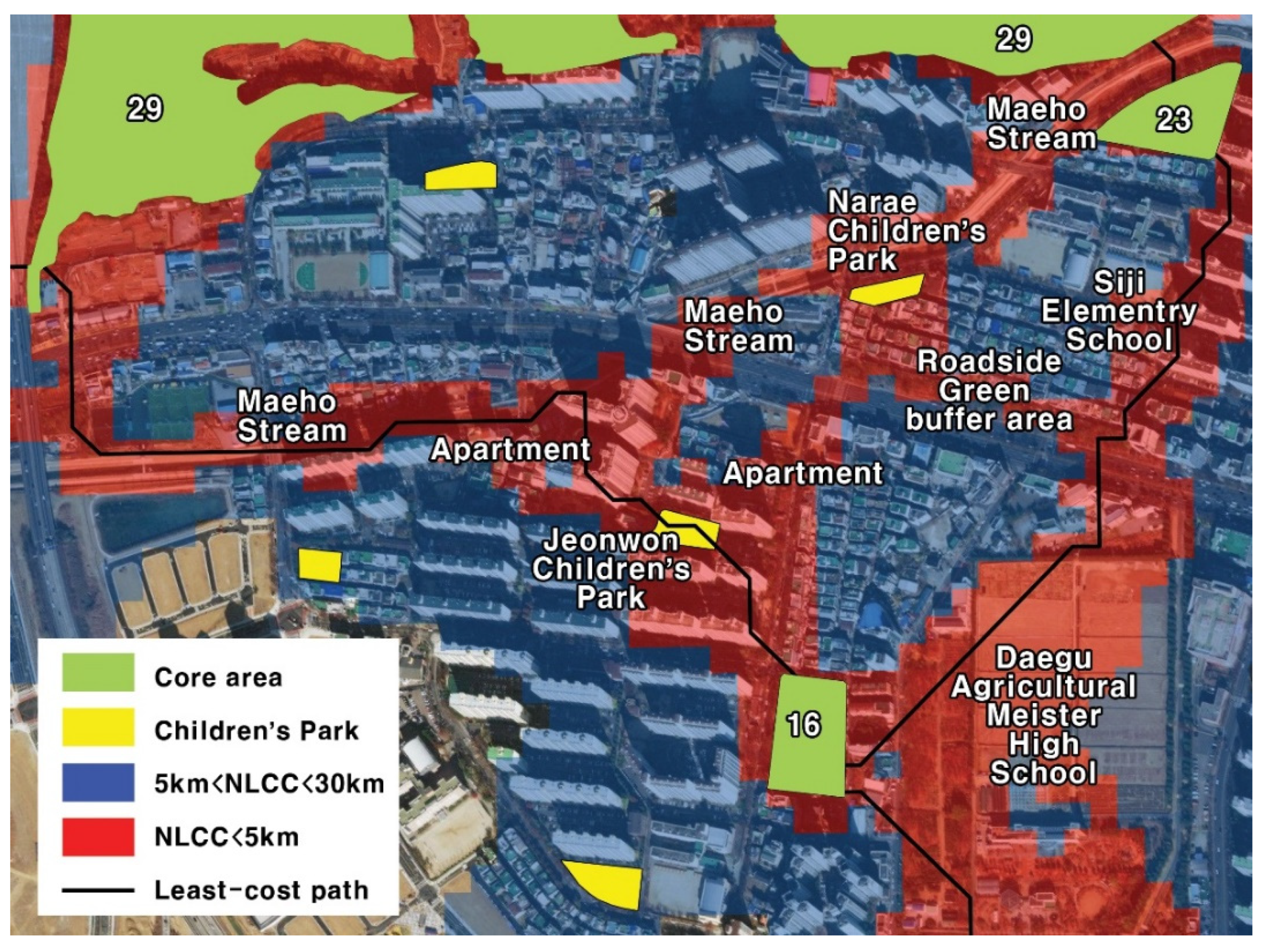
3.3.2. Pinch-Point
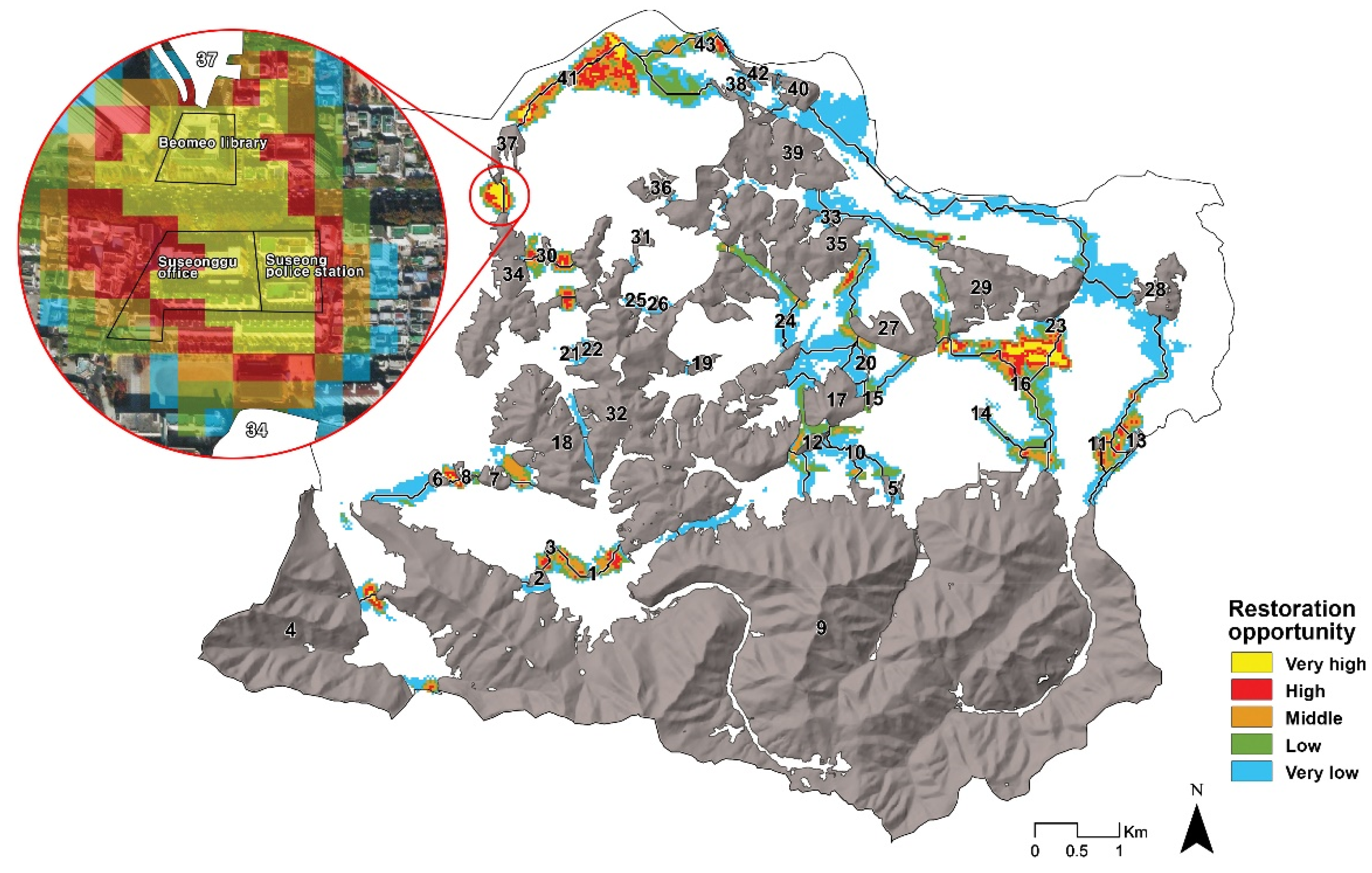
3.3.3. Restoration
4. Discussion
5. Conclusions
Author Contributions
Funding
Conflicts of Interest
Appendix A

| Link ID | Core1 ID | Core2 ID | Link Type | Euc Dist | Lc Dist | eucAdj | cwdAdj | lcpLength | Cwd To EucRatio | Cwd To PathRatio | CF Centrality |
|---|---|---|---|---|---|---|---|---|---|---|---|
| 1 | 1 | 2 | −15 | 427 | 49,586.83 | 1 | 1 | 1458 | 116.13 | 34.01 | −1.00 |
| 2 | 1 | 3 | 1 | 455 | 46,337.44 | 1 | 1 | 531 | 101.84 | 87.26 | 26.41 |
| 3 | 1 | 9 | −15 | 360 | 39,549.96 | 1 | 1 | 1351 | 109.86 | 29.27 | −1.00 |
| 4 | 1 | 32 | 1 | 383 | 34,951.07 | 1 | 1 | 489 | 91.26 | 71.47 | 39.60 |
| 5 | 2 | 3 | 1 | 192 | 21,485.64 | 1 | 1 | 259 | 111.90 | 82.96 | 49.40 |
| 6 | 2 | 9 | 1 | 55 | 662.13 | 1 | 1 | 132 | 12.04 | 5.02 | 88.09 |
| 7 | 3 | 7 | −15 | 813 | 59,373.74 | 1 | 0 | 9536 | 73.03 | 6.23 | −1.00 |
| 8 | 3 | 9 | −15 | 422 | 23,019.02 | 1 | 1 | 634 | 54.55 | 36.31 | −1.00 |
| 9 | 3 | 18 | −15 | 546 | 41,261.89 | 1 | 1 | 8731 | 75.57 | 4.73 | −1.00 |
| 10 | 3 | 32 | −15 | 721 | 34,597.98 | 1 | 1 | 6845 | 47.99 | 5.05 | −1.00 |
| 11 | 4 | 6 | −15 | 1310 | 30,627.79 | 1 | 1 | 3311 | 23.38 | 9.25 | −1.00 |
| 12 | 4 | 9 | 1 | 200 | 19,709.54 | 1 | 1 | 247 | 98.55 | 79.80 | 42.00 |
| 13 | 4 | 34 | −15 | 2242 | 59,066.52 | 1 | 1 | 10,293 | 26.35 | 5.74 | −1.00 |
| 14 | 5 | 9 | 1 | 9 | 424.26 | 1 | 1 | 84 | 47.14 | 5.05 | 73.04 |
| 15 | 5 | 10 | 1 | 343 | 8204.04 | 1 | 1 | 494 | 23.92 | 16.61 | 38.30 |
| 16 | 5 | 14 | −15 | 1093 | 33,363.24 | 1 | 0 | 3443 | 30.52 | 9.69 | −1.00 |
| 17 | 5 | 15 | −15 | 804 | 23,489.91 | 1 | 0 | 6876 | 29.22 | 3.42 | −1.00 |
| 18 | 6 | 7 | −15 | 329 | 25,411.38 | 0 | 1 | 434 | 77.24 | 58.55 | −1.00 |
| 19 | 6 | 8 | 1 | 119 | 19,591.53 | 1 | 1 | 199 | 164.63 | 98.45 | 45.19 |
| 20 | 6 | 9 | 1 | 443 | 6476.65 | 1 | 1 | 836 | 14.62 | 7.75 | 73.31 |
| 21 | 6 | 34 | −15 | 1166 | 49,758.22 | 1 | 1 | 12,788 | 42.67 | 3.89 | −1.00 |
| 22 | 7 | 8 | 1 | 32 | 5157.72 | 1 | 1 | 102 | 161.18 | 50.57 | 49.49 |
| 23 | 7 | 9 | −15 | 761 | 25,339.91 | 1 | 1 | 3007 | 33.30 | 8.43 | −1.00 |
| 24 | 7 | 18 | 1 | 156 | 16,313.53 | 1 | 1 | 294 | 104.57 | 55.49 | 60.85 |
| 25 | 8 | 9 | −15 | 661 | 27,052.14 | 1 | 0 | 1296 | 40.93 | 20.87 | −1.00 |
| 26 | 8 | 18 | −15 | 390 | 22,073.38 | 1 | 1 | 794 | 56.60 | 27.80 | −1.00 |
| 27 | 8 | 34 | −15 | 1007 | 48,007.33 | 1 | 1 | 4964 | 47.67 | 9.67 | −1.00 |
| 28 | 9 | 10 | 1 | 200 | 9307.71 | 1 | 1 | 344 | 46.54 | 27.06 | 33.69 |
| 29 | 9 | 11 | 1 | 556 | 34,110.46 | 1 | 1 | 796 | 61.35 | 42.85 | 33.65 |
| 30 | 9 | 12 | 1 | 452 | 8455.22 | 1 | 1 | 542 | 18.71 | 15.60 | 40.14 |
| 31 | 9 | 13 | 1 | 729 | 14,020.21 | 1 | 1 | 888 | 19.23 | 15.79 | 61.01 |
| 32 | 9 | 14 | 1 | 534 | 25,154.02 | 1 | 1 | 786 | 47.10 | 32.00 | 44.87 |
| 33 | 9 | 16 | 1 | 801 | 39,102.04 | 1 | 1 | 1246 | 48.82 | 31.38 | 33.23 |
| 34 | 9 | 18 | −15 | 900 | 7228.08 | 0 | 1 | 2202 | 8.03 | 3.28 | −1.00 |
| 35 | 9 | 23 | −15 | 1548 | 38,873.07 | 0 | 1 | 6852 | 25.11 | 5.67 | −1.00 |
| 36 | 9 | 28 | −15 | 2190 | 46,525.61 | 0 | 1 | 8163 | 21.24 | 5.70 | −1.00 |
| 37 | 9 | 32 | 1 | 61 | 1176.40 | 1 | 1 | 102 | 19.29 | 11.53 | 273.40 |
| 38 | 9 | 34 | −15 | 1747 | 27,118.63 | 0 | 1 | 4156 | 15.52 | 6.53 | −1.00 |
| 39 | 10 | 12 | 1 | 336 | 3036.58 | 1 | 1 | 422 | 9.04 | 7.20 | 41.12 |
| 40 | 10 | 14 | −15 | 1392 | 43,109.00 | 0 | 1 | 4240 | 30.97 | 10.17 | −1.00 |
| 41 | 10 | 15 | −15 | 428 | 15,266.83 | 1 | 1 | 1411 | 35.67 | 10.82 | −1.00 |
| 42 | 10 | 17 | 1 | 294 | 8461.61 | 1 | 1 | 596 | 28.78 | 14.20 | 44.08 |
| 43 | 11 | 13 | 1 | 314 | 27,090.61 | 1 | 1 | 457 | 86.28 | 59.28 | 26.18 |
| 44 | 11 | 16 | −15 | 1023 | 76,854.59 | 1 | 0 | 2502 | 75.13 | 30.72 | −1.00 |
| 45 | 11 | 23 | −15 | 1334 | 54,662.86 | 1 | 0 | 3461 | 40.98 | 15.79 | −1.00 |
| 46 | 11 | 28 | 1 | 1559 | 46,982.81 | 0 | 1 | 2135 | 30.14 | 22.01 | 28.47 |
| 47 | 12 | 17 | 1 | 76 | 5314.26 | 1 | 1 | 132 | 69.92 | 40.26 | 60.27 |
| 48 | 12 | 32 | 1 | 92 | 6219.44 | 1 | 1 | 157 | 67.60 | 39.61 | 52.04 |
| 49 | 13 | 23 | −15 | 1490 | 55,002.92 | 1 | 0 | 3323 | 36.91 | 16.55 | −1.00 |
| 50 | 13 | 28 | 1 | 1333 | 47,322.86 | 1 | 1 | 1997 | 35.50 | 23.70 | 26.47 |
| 51 | 14 | 15 | −15 | 1084 | 52,881.01 | 1 | 1 | 9333 | 48.78 | 5.67 | −1.00 |
| 52 | 14 | 16 | 1 | 442 | 51,640.21 | 1 | 1 | 1823 | 116.83 | 28.33 | 25.48 |
| 53 | 14 | 27 | −15 | 827 | 54,795.02 | 1 | 1 | 9413 | 66.26 | 5.82 | −1.00 |
| 54 | 14 | 29 | −15 | 847 | 67,691.33 | 1 | 1 | 10,649 | 79.92 | 6.36 | −1.00 |
| 55 | 15 | 17 | 1 | 51 | 5374.26 | 1 | 1 | 132 | 105.38 | 40.71 | 35.17 |
| 56 | 15 | 20 | 1 | 128 | 6093.20 | 1 | 1 | 252 | 47.60 | 24.18 | 23.67 |
| 57 | 15 | 27 | 1 | 520 | 12,452.56 | 1 | 1 | 646 | 23.95 | 19.28 | 30.94 |
| 58 | 16 | 23 | 1 | 668 | 80,671.99 | 1 | 1 | 941 | 120.77 | 85.73 | 18.90 |
| 59 | 16 | 29 | 1 | 681 | 77,417.98 | 1 | 1 | 1264 | 113.68 | 61.25 | 19.54 |
| 60 | 17 | 20 | 1 | 145 | 1236.40 | 1 | 1 | 174 | 8.53 | 7.11 | 79.72 |
| 61 | 17 | 27 | 1 | 441 | 8491.46 | 1 | 1 | 506 | 19.26 | 16.78 | 41.96 |
| 62 | 17 | 32 | 1 | 45 | 4090.14 | 1 | 1 | 489 | 90.89 | 8.36 | 98.84 |
| 63 | 18 | 21 | −15 | 242 | 4890.73 | 1 | 1 | 1236 | 20.21 | 3.96 | −1.00 |
| 64 | 18 | 32 | 1 | 26 | 450.00 | 1 | 1 | 60 | 17.31 | 7.50 | 98.87 |
| 65 | 18 | 34 | −15 | 267 | 23,982.28 | 1 | 1 | 3062 | 89.82 | 7.83 | −1.00 |
| 66 | 19 | 32 | 1 | 33 | 210.00 | 1 | 1 | 60 | 6.36 | 3.50 | 42.00 |
| 67 | 20 | 27 | 1 | 164 | 8054.77 | 1 | 1 | 319 | 49.11 | 25.25 | 44.23 |
| 68 | 21 | 22 | 1 | 19 | 150.00 | 1 | 1 | 60 | 7.89 | 2.50 | 42.00 |
| 69 | 21 | 32 | −15 | 74 | 859.71 | 1 | 1 | 204 | 11.62 | 4.21 | −1.00 |
| 70 | 21 | 34 | −15 | 248 | 21,950.44 | 1 | 1 | 1820 | 88.51 | 12.06 | −1.00 |
| 71 | 22 | 32 | 1 | 28 | 540.00 | 1 | 1 | 60 | 19.29 | 9.00 | 82.00 |
| 72 | 22 | 34 | −15 | 354 | 21,630.73 | 1 | 1 | 1676 | 61.10 | 12.91 | −1.00 |
| 73 | 23 | 28 | −15 | 872 | 8755.62 | 1 | 1 | 1480 | 10.04 | 5.92 | −1.00 |
| 74 | 23 | 29 | 1 | 48 | 543.20 | 1 | 1 | 72 | 11.32 | 7.54 | 57.38 |
| 75 | 24 | 27 | −15 | 632 | 16,272.49 | 1 | 0 | 1259 | 25.75 | 12.92 | −1.00 |
| 76 | 24 | 32 | 1 | 187 | 2803.68 | 1 | 1 | 367 | 14.99 | 7.64 | 119.71 |
| 77 | 24 | 35 | 1 | 231 | 7159.30 | 1 | 1 | 289 | 30.99 | 24.77 | 101.67 |
| 78 | 25 | 26 | −15 | 78 | 2079.59 | 1 | 1 | 204 | 26.66 | 10.19 | −1.00 |
| 79 | 25 | 32 | 1 | 35 | 724.26 | 1 | 1 | 72 | 20.69 | 10.06 | 42.00 |
| 80 | 26 | 31 | −15 | 396 | 3906.76 | 1 | 1 | 1006 | 9.87 | 3.88 | −1.00 |
| 81 | 26 | 32 | 1 | 33 | 424.26 | 1 | 1 | 42 | 12.86 | 10.10 | 42.00 |
| 82 | 27 | 29 | 1 | 120 | 9906.24 | 1 | 1 | 174 | 82.55 | 56.93 | 86.43 |
| 83 | 27 | 32 | 1 | 584 | 13,082.89 | 1 | 1 | 849 | 22.40 | 15.41 | 43.12 |
| 84 | 27 | 35 | 1 | 514 | 20,349.66 | 1 | 1 | 1116 | 39.59 | 18.23 | 41.82 |
| 85 | 28 | 29 | 1 | 582 | 7160.10 | 1 | 1 | 761 | 12.30 | 9.41 | 74.68 |
| 86 | 29 | 35 | 1 | 882 | 17,681.61 | 1 | 1 | 1121 | 20.05 | 15.77 | 49.12 |
| 87 | 29 | 39 | 1 | 1339 | 21,374.10 | 1 | 0 | 1813 | 15.96 | 11.79 | 42.03 |
| 88 | 29 | 40 | 1 | 2258 | 24,784.57 | 1 | 0 | 4822 | 10.98 | 5.14 | 39.32 |
| 89 | 30 | 32 | 1 | 173 | 22,367.82 | 1 | 1 | 264 | 129.29 | 84.73 | 49.67 |
| 90 | 30 | 34 | 1 | 165 | 15,151.83 | 1 | 1 | 234 | 91.83 | 64.75 | 44.20 |
| 91 | 30 | 37 | −15 | 816 | 77,553.54 | 1 | 1 | 1276 | 95.04 | 60.78 | −1.00 |
| 92 | 31 | 32 | 1 | 38 | 543.20 | 1 | 1 | 72 | 14.29 | 7.54 | 42.00 |
| 93 | 31 | 36 | −15 | 306 | 19,511.79 | 1 | 1 | 4235 | 63.76 | 4.61 | −1.00 |
| 94 | 31 | 39 | −15 | 253 | 16,643.85 | 1 | 1 | 3663 | 65.79 | 4.54 | −1.00 |
| 95 | 32 | 34 | 1 | 158 | 17,100.00 | 1 | 1 | 210 | 108.23 | 81.43 | 72.46 |
| 96 | 32 | 35 | 1 | 70 | 5550.00 | 1 | 1 | 120 | 79.29 | 46.25 | 167.34 |
| 97 | 32 | 36 | −15 | 377 | 10,198.60 | 1 | 1 | 1730 | 27.05 | 5.90 | −1.00 |
| 98 | 32 | 37 | −15 | 1078 | 83,168.29 | 1 | 1 | 2336 | 77.15 | 35.60 | −1.00 |
| 99 | 32 | 39 | −15 | 282 | 7330.66 | 1 | 1 | 1158 | 26.00 | 6.33 | −1.00 |
| 100 | 33 | 35 | 1 | 19 | 212.13 | 1 | 1 | 42 | 11.16 | 5.05 | 53.41 |
| 101 | 33 | 39 | 1 | 270 | 3075.99 | 1 | 1 | 349 | 11.39 | 8.81 | 17.91 |
| 102 | 34 | 37 | 1 | 332 | 60,598.33 | 1 | 1 | 414 | 182.53 | 146.37 | 50.76 |
| 103 | 35 | 39 | 1 | 10 | 212.13 | 1 | 1 | 42 | 21.21 | 5.05 | 235.68 |
| 104 | 35 | 40 | −15 | 1035 | 4548.31 | 0 | 1 | 1351 | 4.39 | 3.37 | −1.00 |
| 105 | 36 | 37 | −15 | 1276 | 102,689.28 | 1 | 1 | 6571 | 80.48 | 15.63 | −1.00 |
| 106 | 36 | 39 | 1 | 12 | 127.28 | 1 | 1 | 42 | 10.61 | 3.03 | 42.00 |
| 107 | 36 | 41 | −15 | 1341 | 156,429.06 | 1 | 1 | 4460 | 116.65 | 35.07 | −1.00 |
| 108 | 37 | 41 | 1 | 722 | 84,507.27 | 1 | 1 | 821 | 117.05 | 102.93 | 35.35 |
| 109 | 38 | 39 | 1 | 36 | 724.26 | 1 | 1 | 72 | 20.12 | 10.06 | 126.40 |
| 110 | 38 | 42 | 1 | 51 | 724.26 | 1 | 1 | 72 | 14.20 | 10.06 | 102.72 |
| 111 | 39 | 40 | 1 | 151 | 2834.92 | 1 | 1 | 217 | 18.77 | 13.06 | 53.01 |
| 112 | 39 | 41 | 1 | 1571 | 149,454.09 | 1 | 1 | 2172 | 95.13 | 68.81 | 24.87 |
| 113 | 39 | 42 | −15 | 210 | 2297.06 | 1 | 1 | 302 | 10.94 | 7.61 | −1.00 |
| 114 | 39 | 43 | −15 | 307 | 18,560.35 | 1 | 1 | 978 | 60.46 | 18.98 | −1.00 |
| 115 | 40 | 42 | 1 | 12 | 1360.66 | 1 | 1 | 114 | 113.39 | 11.94 | 66.37 |
| 116 | 41 | 43 | 1 | 1458 | 140,899.64 | 1 | 1 | 1763 | 96.64 | 79.92 | 26.25 |
| 117 | 42 | 43 | 1 | 147 | 14,863.40 | 1 | 1 | 446 | 101.11 | 33.33 | 61.17 |
References
- Forman, R.T.T. Urban Ecology: Science of Cites, 1st ed.; Cambridge University Press: Cambridge, UK, 2014. [Google Scholar]
- Kang, S.; Kim, J.O. Morphological analysis of green infrastructure in the Seoul metropolitan area, South Korea. Landsc. Ecol. Eng. 2015, 11, 259–268. [Google Scholar] [CrossRef]
- Ra, J.H. Possibility and limitations of new framework of landscape ecology. J. Korean Inst. Landsc. Archit. 2005, 33, 45–70. [Google Scholar]
- Harris, L.D.; Scheck, J. From implications to applications: The dispersal corridor principle applied to the conservation of biological diversity. Nat. Conserv. 1991, 2, 189–220. [Google Scholar]
- Jongman, R. Ecological networks are an issue for all of us. J. Landsc. Ecol. 2008, 1, 7–13. [Google Scholar] [CrossRef] [Green Version]
- Niemelä, J.; Saarela, S.R.; Söderman, T.; Kopperoinen, L.; Yli-Pelkonen, V.; Väre, S.; Kotze, D.J. Using the ecosystem services approach for better planning and conservation of urban green spaces: A Finland case study. Biodivers. Conserv. 2010, 19, 3225–3243. [Google Scholar] [CrossRef]
- Wei, J.; Qian, J.; Tao, Y.; Hu, F.; Ou, W. Evaluating spatial priority of urban green infrastructure for urban sustainability in areas of rapid urbanization: A case study of Pukou in China. Sustainability 2018, 10, 327. [Google Scholar] [CrossRef] [Green Version]
- Huang, B.X.; Chiou, S.C.; Li, W.Y. Landscape Pattern and Ecological Network Structure in Urban Green Space Planning: A Case Study of Fuzhou City. Land 2021, 10, 769. [Google Scholar] [CrossRef]
- Kong, F.; Yin, H.; Nakagoshi, N.; Zong, Y. Urban green space network development for biodiversity conservation: Identification based on graph theory and gravity modeling. Landsc. Urban Plan. 2010, 95, 16–27. [Google Scholar] [CrossRef]
- Moseley, D.; Marzano, M.; Chetcuti, J.; Watts, K. Green networks for people: Application of a functional approach to support the planning and management of greenspace. Landsc. Urban Plan. 2013, 116, 1–12. [Google Scholar] [CrossRef]
- Sagong, J.H. Development of Landscape Ecological Green-Network Model in a Metropolitan. Ph.D. Thesis, Kyungpook National University, Daegu, Korea, 2004. [Google Scholar]
- Han, B.H.; Kwak, J.I.; Park, S.C.; Hur, J.Y. A study on planning of roadside green for enhancing urban green network. Korean J. Environ. Ecol. 2014, 28, 128–141. [Google Scholar] [CrossRef]
- Nowicki, P.; Bennett, G.; Middleton, D.; Rientjes, S.; Wolters, R. Perspectives on Ecological Networks; European Center of Nature Conservation: Arnhem, The Netherlands, 2006. [Google Scholar]
- Fahrig, L. Effects of habitat fragmentation on biodiversity. Annu. Rev. Ecol. Evol. Syst. 2003, 34, 487–515. [Google Scholar] [CrossRef] [Green Version]
- Etherington, T.R. Geographical isolation and invasion ecology. Prog. Phys. Geogr. 2015, 39, 697–710. [Google Scholar] [CrossRef]
- Ostfeld, R.S.; Glass, G.E.; Keesing, F. Spatial epidemiology: An emerging (or re-emerging) discipline. Trends Ecol. Evol. 2005, 20, 328–336. [Google Scholar] [CrossRef]
- Meentemeyer, R.K.; Haas, S.E.; Václavík, T. Landscape epidemiology of emerging infectious diseases in natural and human-altered ecosystems. Annu. Rev. Phytopathol. 2012, 50, 379–402. [Google Scholar] [CrossRef] [Green Version]
- Wilson, E.O.; MacArthur, R.H. The Theory of Island Biogeography; Princeton University Press: Princeton, NJ, USA, 1967. [Google Scholar]
- Forman, R.T.; Godron, M. Patches and structural components for a landscape ecology. BioScience 1981, 31, 733–740. [Google Scholar]
- Opdam, P.; van Dorp, D.T.; Ter Braak, D.J.F. The effect of isolation on the number of woodland birds in small woods in the Netherlands. J. Biogeogr. 1984, 11, 473–478. [Google Scholar] [CrossRef]
- Thomas, C.D.; Thomas, J.A.; Warren, M.S. Distributions of occupied and vacant butterfly habitats in fragmented landscapes. Oecologia 1992, 92, 563–567. [Google Scholar] [CrossRef]
- Taylor, P.D.; Fahrig, L.; Henein, K.; Merriam, G. Connectivity is a vital element of landscape structure. Oikos 1993, 68, 571–573. [Google Scholar] [CrossRef] [Green Version]
- Ricketts, T.H. The matrix matters: Effective isolation in fragmented landscapes. Am. Nat. 2001, 158, 87–99. [Google Scholar] [CrossRef]
- Warntz, W. Transportation, social physics, and the law of refraction. Prof. Geogr. 1957, 9, 2–7. [Google Scholar] [CrossRef]
- Chardon, J.P.; Adriaensen, F.; Matthysen, E. Incorporating landscape elements into a connectivity measure: A case study for the Speckled wood butterfly (Pararge aegeria L.). Landsc. Ecol. 2003, 18, 561–573. [Google Scholar] [CrossRef]
- Verbeylen, G.; De Bruyn, L.; Adriaensen, F.; Matthysen, E. Does matrix resistance influence red squirrel (Sciurus vulgaris L. 1758) distribution in an urban landscape? Landsc Ecol. 2003, 18, 791–805. [Google Scholar] [CrossRef]
- Etherington, T.R. Least-cost modelling and landscape ecology: Concepts, applications, and opportunities. Current Landscape Ecology Reports. 2016, 1, 40–53. [Google Scholar] [CrossRef] [Green Version]
- Balbi, M.; Petit, E.J.; Croci, S.; Nabucet, J.; Georges, R.; Madec, L.; Ernoult, A. Ecological relevance of least cost path analysis: An easy implementation method for landscape urban planning. J. Environ. Manag. 2019, 244, 61–68. [Google Scholar] [CrossRef]
- Blair, R.B. Land use and avian species diversity along an urban gradient. Ecol. Appl. 1996, 6, 506–519. [Google Scholar] [CrossRef]
- Hong, S.H.; Han, B.H.; Choi, S.H.; Sung, C.Y.; Lee, K.J. Planning an ecological network using the predicted movement paths of urban birds. Landsc. Ecol. Eng. 2013, 9, 165–174. [Google Scholar] [CrossRef]
- Meffert, P.J.; Dziock, F. The influence of urbanisation on diversity and trait composition of birds. Landsc. Ecol. 2013, 28, 943–957. [Google Scholar] [CrossRef]
- Sandström, U.G.; Angelstam, P.; Mikusiński, G. Ecological diversity of birds in relation to the structure of urban green space. Landsc. Urban Plan. 2006, 77, 39–53. [Google Scholar] [CrossRef]
- Mörtberg, U.; Wallentinus, H.G. Red-listed forest bird species in an urban environment—Assessment of green space corridors. Landsc. Urban Plan. 2000, 50, 215–226. [Google Scholar] [CrossRef]
- Ministry of Environment. 2nd National Natural Environment Survey Report; Ministry of Environment: Gwacheon, Korea, 2000.
- Ministry of Environment. 3rd National Natural Environment Survey Report; Ministry of Environment: Gwacheon, Korea, 2009.
- Šálek, M.; Drahníková, L.; Tkadlec, E. Changes in home range sizes and population densities of carnivore species along the natural to urban habitat gradient. Mammal Rev. 2015, 45, 1–14. [Google Scholar] [CrossRef]
- Park, C.R.; Choi, M.S. Comparison of bird communities at urban forests and streetscapes in Daegu city. Korean J. Environ. Ecol. 2005, 19, 367–374. [Google Scholar]
- Yun, M.B. Resident Bird of Korea; Daewonsa: Seoul, Korea, 1993. [Google Scholar]
- Summers-Smith, J.D. The Sparrows: A Study of the Genus Passer; T & AD Poyser: Staffordshier, UK, 1988. [Google Scholar]
- Groschupf, K. Old World Sparrows. In The Sibley Guide to Bird Life and Behavior, 1st ed.; Elphick, C., Dunning, J.B., Sibley, D.A., Eds.; Alfred A. Knopf: New York City, NY, USA, 2000; pp. 562–564. [Google Scholar]
- Campbell, B.; Lack, E. A Dictionary of Birds; A&C Black: London, UK, 1985. [Google Scholar]
- Wilcox, B.A. In situ conservation of genetic resources: Determinants of minimum area requirements. In National Parks, Conservation and Development: The Role of Protected Areas in Sustaining Society; McNeely, J.A., Miller, K., Eds.; Smithsonian Institution Press: Washington, DC, USA, 1984; pp. 639–647. [Google Scholar]
- Kohn, D.D.; Walsh, D.M. Plant species richness—The effect of island size and habitat diversity. J. Ecol. 1994, 82, 367–377. [Google Scholar] [CrossRef]
- Riess, W. Konzepte zum Biotopverbund im Arten-und Biotopschutzprogramm Bayern. Lauf. Semin. 1986, 10, 102–115. [Google Scholar]
- Baker, W.L.; Cai, Y. The r.le programs for multiscale analysis of landscape structure using the GRASS geographical information system. Landsc. Ecol. 1992, 7, 291–302. [Google Scholar] [CrossRef]
- McGarigal, K. FRAGSTATS: Spatial Pattern Analysis Program for Quantifying Landscape Structure; US Department of Agriculture, Forest Service, Pacific Northwest Research Station: Portland, OR, USA, 1995.
- Matte, A.L.L.; Müller, S.C.; Becker, F.G. Forest expansion or fragmentation? Discriminating forest fragments from natural forest patches through patch structure and spatial context metrics. Austral Ecol. 2015, 40, 21–31. [Google Scholar] [CrossRef]
- Alphan, H.; Çelik, N. Monitoring changes in landscape pattern: Use of Ikonos and Quickbird images. Environ. Monit. Assess. 2016, 188, 81. [Google Scholar] [CrossRef]
- Singleton, P.H. Landscape Permeability for Large Carnivores in Washington: A Geographic Information System Weighted-Distance and Least-Cost Corridor Assessment; US Department of Agriculture, Forest Service: Portland, OR, USA, 2002; Volume 549.
- Adrensen, F.; Chardon, J.P.; De Blust, G.; Swinnen, E.; Villalba, S.; Gulinck, H.; Mattysen, E. The application of ‘least-cost’modelling as a functional landscape model. Landsc. Urban Plan. 2003, 64, 233–247. [Google Scholar] [CrossRef]
- Belote, R.T.; Dietz, M.S.; McRae, B.H.; Theobald, D.M.; McClure, M.L.; Urwin, G.H.; Aplete, G.H. Identifying corridors among large protected areas in the United States. PLoS ONE 2016, 11, e0154223. [Google Scholar] [CrossRef] [Green Version]
- Penrod, K.; Cabañero, C.; Beier, P.; Luke, C.; Spencer, W.; Rubin, E.; Remson, E. South Coast Missing Linkages Project: A Linkage Design for the Santa Monica-Sierra Madre Connection; South Coast Wildlands: Idyllwild, CA, USA, 2006. [Google Scholar]
- Tremblay, M.A.; St. Clair, C.C. Permeability of a heterogeneous urban landscape to the movements of forest songbirds. J. Appl. Ecol. 2011, 48, 679–688. [Google Scholar] [CrossRef]
- Shimazaki, A.; Yamaura, Y.; Senzaki, M.; Yabuhara, Y.; Akasaka, T.; Nakamura, F. Urban permeability for birds: An approach combining mobbing-call experiments and circuit theory. Urban For. Urban Green. 2016, 19, 167–175. [Google Scholar] [CrossRef]
- Watts, K.; Eycott, A.E.; Handley, P.; Ray, D.; Humphrey, J.W.; Quine, C.P. Targeting and evaluating biodiversity conservation action within fragmented landscapes: An approach based on generic focal species and least-cost networks. Landsc. Ecol. 2010, 25, 1305–1318. [Google Scholar] [CrossRef]
- United States Geological Survey (USGS). Available online: http://earthexplorer.usgs.gov (accessed on 7 May 2020).
- Daegu Map Portal. Available online: http://gis.go.kr (accessed on 27 April 2020).
- Singleton, P.H.; Gaines, W.L.; Lehmkuhl, J.F. Landscape permeability for grizzly bear movements in Washington and southwestern British Columbia. Ursus 2004, 15, 90–103. [Google Scholar] [CrossRef]
- McRae, B.H.; Dickson, B.G.; Keitt, T.H.; Shah, V.B. Using circuit theory to model connectivity in ecology, evolution, and conservation. Ecology 2008, 89, 2712–2724. [Google Scholar] [CrossRef]
- McRae, B.H. Centrality Mapper Connectivity Analysis Software; The Nature Conservcancy: Seattle, WA, USA, 2012; Available online: http://www.circuitscape.org/linkagemapper (accessed on 11 May 2020).
- McRae, B.H.; Shah, V.B. Circuitscape User’s Guide; The University of California: Snata Babara, CA, USA, 2009. [Google Scholar]
- McRae, B.H. Pinchpoint Mapper Connectivity Analysis Software; The Nature Conservancy: Seattle, WA, USA, 2012; Available online: http://www.circuitscape.org/linkagemapper (accessed on 11 May 2020).
- McRae, B.H. Barrier Mapper Connectivity Analysis Software; The Nature Conservancy: Seattle, WA, USA, 2012; Available online: http://www.circuitscape.org/linkagemapper (accessed on 11 May 2020).
- Forman, R.T. Land Mosaics: The Ecology of Landscape and Regions; Island Press: Washington DC, USA, 1995. [Google Scholar]
- Bunn, A.G.; Urban, D.L.; Keitt, T.H. Landscape connectivity: A conservation application of graph theory. J. Environ. Manag. 2000, 59, 265–278. [Google Scholar] [CrossRef] [Green Version]
- Zetterberg, A.; Mörtberg, U.M.; Balfors, B. Making graph theory operational for landscape ecological assessments, planning, and design. Landsc. Urban Plan. 2010, 95, 181–191. [Google Scholar] [CrossRef]
- Arif, K.; Afzal, Z.; Nadeem, M.; Ahmad, B.; Mahmood, A.; Iqbal, M.; Nazir, A. Role of graph theory to facilitate landscape connectivity: Subdivision of a Harary graph. Pol. J. Environ. Stud. 2018, 27, 993–999. [Google Scholar] [CrossRef]
- Rudd, H.; Vala, J.; Schaefer, V. Importance of backyard habitat in a comprehensive biodiversity conservation strategy: A connectivity analysis of urban green spaces. Restor. Ecol. 2002, 10, 368–375. [Google Scholar] [CrossRef] [Green Version]
- Yang, H.; Chen, W.; Chen, X. Regional Ecological Network Planning for Biodiversity Conservation: A Case Study of China’s Poyang Lake Eco-Economic Region. Pol. J. Environ. Stud. 2017, 26, 1825–1833. [Google Scholar] [CrossRef]
- Pelorosso, R.; Gobattoni, F.; Geri, F.; Monaco, R.; Leone, A. Evaluation of Ecosystem Services related to Bio-Energy Landscape Connectivity (BELC) for land use decision making across different planning scales. Ecol. Indic. 2016, 61, 114–129. [Google Scholar] [CrossRef]
- de Souza Leite, M.; Tambosi, L.R.; Romitelli, I.; Metzger, J.P. Landscape ecology perspective in restoration projects for biodiversity conservation: A review. Nat. Conserv. 2013, 11, 108–118. [Google Scholar] [CrossRef]
- Klaus, V.H.; Kiehl, K. A conceptual framework for urban ecological restoration and rehabilitation. Basic Appl. Ecol. 2021, 52, 82–94. [Google Scholar] [CrossRef]
- Hou, W.; Zhai, L.; Feng, S.; Walz, U. Restoration priority assessment of coal mining brownfields from the perspective of enhancing the connectivity of green infrastructure networks. J. Environ. Manag. 2021, 277, 111289. [Google Scholar] [CrossRef] [PubMed]
- Hermoso, V.; Villero, D.; Clavero, M.; Brotons, L. Spatial prioritisation of EU’s LIFE-Nature programme to strengthen the conservation impact of Natura 2000. J. Appl. Ecol. 2018, 55, 1575–1582. [Google Scholar] [CrossRef] [Green Version]
- Srinivasulu, A.; Srinivasulu, B.; Srinivasulu, C. Ecological niche modelling for the conservation of endemic threatened squamates (lizards and snakes) in the Western Ghats. Glob. Ecol. Conserv. 2021, 28, e01700. [Google Scholar] [CrossRef]
- Verhagen, W.; Kukkala, A.S.; Moilanen, A.; van Teeffelen, A.J.; Verburg, P.H. Use of demand for and spatial flow of ecosystem services to identify priority areas. Conserv. Biol. 2017, 31, 860–871. [Google Scholar] [CrossRef]
- Lee, S.W. The impacts of greenbelt policies on anti-sprawl. J. Korea Plan. Assoc. 2018, 53, 45–65. [Google Scholar] [CrossRef] [Green Version]
- Ryu, D.H.; Lee, D.K. Evaluation on economic value of the greenbelt’s ecosystem services in the Seoul metropolitan region. J. Korea Plan. Assoc. 2013, 48, 279–292. [Google Scholar]
- Merrick, M.J.; Koprowski, J.L. Circuit theory to estimate natal dispersal routes and functional landscape connectivity for an endangered small mammal. Landsc. Ecol. 2017, 32, 1163–1179. [Google Scholar] [CrossRef]
- Campos, F.S.; Lourenço-de-Moraes, R.; Ruas, D.S.; Mira-Mendes, C.V.; Franch, M.; Llorente, G.A.; Cabral, P. Searching for networks: Ecological connectivity for amphibians under climate change. Environ. Manag. 2020, 65, 46–61. [Google Scholar] [CrossRef]
- Saito, M.; Momose, H.; Mihira, T. Both environmental factors and countermeasures affect wild boar damage to rice paddies in Boso Peninsula, Japan. Crop Prot. 2011, 30, 1048–1054. [Google Scholar] [CrossRef]
- Herrera, J.; Nunn, C.L. Behavioural ecology and infectious disease: Implications for conservation of biodiversity. Philos. Trans. R. Soc. B 2019, 374, 20180054. [Google Scholar] [CrossRef] [Green Version]


| NDVI | Definition | Weighted Value |
|---|---|---|
| NDVI < 0.2 | Vegetation does not exist | 10 |
| 0.2 ≤ NDVI < 0.5 | Vegetation density is low | 5 |
| 0.5 ≤ NDVI | Vegetation density is high | 1 |
| Electrical Term (Symbol, Unit) | Ecological Interpretation |
|---|---|
| Resistance (R, ohm) the opposition that a resistor offers to the flow of electrical current. | Opposition of a habitat type to movement of organisms, similar to ecological concepts of landscape resistance or friction. Grid cells allowing less movement are assigned higher resistance. |
| Current (I, amp) flow of charge through a node or resistor in a circuit. | Current through nodes or resistors can be used to predict expected net movement probabilities for random walkers moving through corresponding core areas or paths. |
| Voltage (V, volt) the potential difference in electrical charge between two nodes in an electrical circuit. | Voltages can be used to predict the probability that random walkers leaving any point on a green network will reach a given destination (representing, e.g., successful dispersal) before another. |
Publisher’s Note: MDPI stays neutral with regard to jurisdictional claims in published maps and institutional affiliations. |
© 2021 by the authors. Licensee MDPI, Basel, Switzerland. This article is an open access article distributed under the terms and conditions of the Creative Commons Attribution (CC BY) license (https://creativecommons.org/licenses/by/4.0/).
Share and Cite
Kwon, O.-S.; Kim, J.-H.; Ra, J.-H. Landscape Ecological Analysis of Green Network in Urban Area Using Circuit Theory and Least-Cost Path. Land 2021, 10, 847. https://doi.org/10.3390/land10080847
Kwon O-S, Kim J-H, Ra J-H. Landscape Ecological Analysis of Green Network in Urban Area Using Circuit Theory and Least-Cost Path. Land. 2021; 10(8):847. https://doi.org/10.3390/land10080847
Chicago/Turabian StyleKwon, Oh-Sung, Jin-Hyo Kim, and Jung-Hwa Ra. 2021. "Landscape Ecological Analysis of Green Network in Urban Area Using Circuit Theory and Least-Cost Path" Land 10, no. 8: 847. https://doi.org/10.3390/land10080847
APA StyleKwon, O.-S., Kim, J.-H., & Ra, J.-H. (2021). Landscape Ecological Analysis of Green Network in Urban Area Using Circuit Theory and Least-Cost Path. Land, 10(8), 847. https://doi.org/10.3390/land10080847