Identifying Potential Cropland Losses When Conserving 30% and 50% Earth with Different Approaches and Spatial Scales

Abstract

Biodiversity conservation is the cornerstone for sustainable development. Bold conservation targets provide the last opportunities to halt the human-driven mass extinction. Recently, bold conservation targets have been proposed to protect 30% or 50% of Earth. However, little is known about its potential impacts on cropland. We identify potential cropland losses when 30% and 50% of global terrestrial area is given back to nature by 2030/2050, at three spatial scales (global, biome and country) and using two approaches (“nature-only landscapes” and “shared landscapes”). We find that different targets, applied scales and approaches will lead to different cropland losses: (1) At the global scale, it is possible to protect 50% of the Earth while having minimum cropland losses. (2) At biome scale, 0.64% and 8.54% cropland will be lost globally in 2030 and 2050 under the nature-only approach while by contrast, the shared approach substantially reduces the number of countries confronted by cropland losses, demanding only 0% and 2.59% of global cropland losses in 2030 and 2050. (3) At the national scale, the nature-only approach causes losses of 3.58% and 10.73% of global cropland in 2030 and 2050, while the shared approach requires 0.77% and 7.55% cropland in 2030 and 2050. Our results indicate that bold conservation targets could be considered, especially when adopting the shared approach, and we suggest adopting ambitious targets (protecting at least 30% by 2030) at the UN Biodiversity Conference (COP 15) to ensure a sustainable future for Earth.

1. Introduction

Human-driven biodiversity crisis caused by humankind is one of the most severe challenges to sustainable development [1,2,3,4]. To bend the curve of biodiversity loss, calls have been made for expanding protected areas and leaving more space for nature [5,6]. In this context, increasingly ambitious, area-based conservation targets (e.g., 30% or 50% of all land) are being promoted globally to stem the rising tide of biodiversity loss, such as the Nature Needs Half initiative (2009) [7] and the Half-Earth project (2016) [8]. Relevant discussion is going on and what we have learned is that: the current protected areas system is not enough to bend the curve of biodiversity loss and we need bold conservation targets [9]. However, what we do not know is where we should expand protected areas and what are the potential impacts of those bold conservation targets [6]. Although the feasibility of bold conservation targets has been analyzed from a certain perspective [10], few spatial analyses exist in assessing its potential impacts on cropland [11]. In fact, food security and biodiversity conservation are interrelated challenges [12,13]. Besides conserving Earth’s remaining intact ecosystems [14], giving farmlands back to nature could also make contributions to conservation which may threaten food security. Currently, conversion of cropland to natural habitat takes place across the world, which may have complex effects on biodiversity [15,16,17], while farmland abandonment would make more space for nature conservation in general [17,18,19].

The Aichi target 11 proposed in 2010 calls for protection of 17% terrestrial land but biodiversity is still declining, and the 15th Meeting of the Conference of the Parties to the Convention on Biological Diversity (CBD) will be held in China to adopt the post-2020 global biodiversity framework (GBF). In recent years, calls have been made for protecting 30% of the Earth by 2030 and 50% by 2050 (known as 30 by 30 and 50 by 50). However, we know little about the potential impacts of bold conservation targets on cropland losses, thus it is crucial to predict future impacts of bold conservation target setting on cropland through spatially explicit analyses.

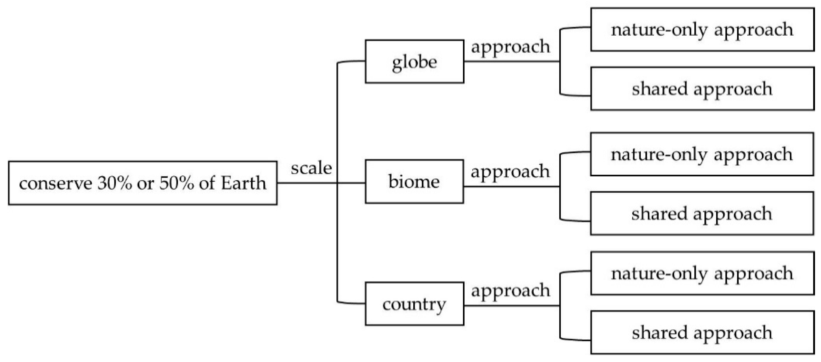
We identify potential cropland losses when bold conservation targets are applied considering multiple scenarios. First, we identify potential cropland losses at three spatial scales, including global, biome and the national scales, by adopting the model developed in Mehrabi et al., 2018. Second, considering the suggestions from the conservation community, we set a goal of allocating 30% and 50% of global terrestrial land for conservation by 2030 and 2050, respectively [20]. Third, we apply two conservation approaches (‘nature-only’ and ‘shared’) to simulate cropland losses under different future scenarios. ‘Nature-only landscapes’ are landscapes where conservation displaces all crop production in a landscape unit (~8.4 km × 8.4 km pixel), while ‘shared landscapes’ are regions where conservation and crop production are allowed to coexist within each landscape unit (~8.4 km × 8.4 km pixel) [21]. Under the above scenarios and based on land use and caloric supply, we minimize the cropland losses due to conservation. Compared to previous studies, our analysis contributes to the literature by incorporating data on future land use and land cover, and simulating multiple scenarios to get a more comprehensive understanding on this issue.

2. Materials and Methods

There are five steps for conducting the analyses, including defining land classes, defining pixel types, calculating calories of pixels, identifying conservation areas according to ranking of pixels and land classes, and identifying potential cropland losses. All datasets are processed to have a resolution of 8.4 km under Eckert IV’s equal-area projection, since we follow the methods in Mehrabi et al., 2018 and have to match other datasets with the 5-arc-minute calorie dataset.

2.1. Step 1: Defining Land Classes

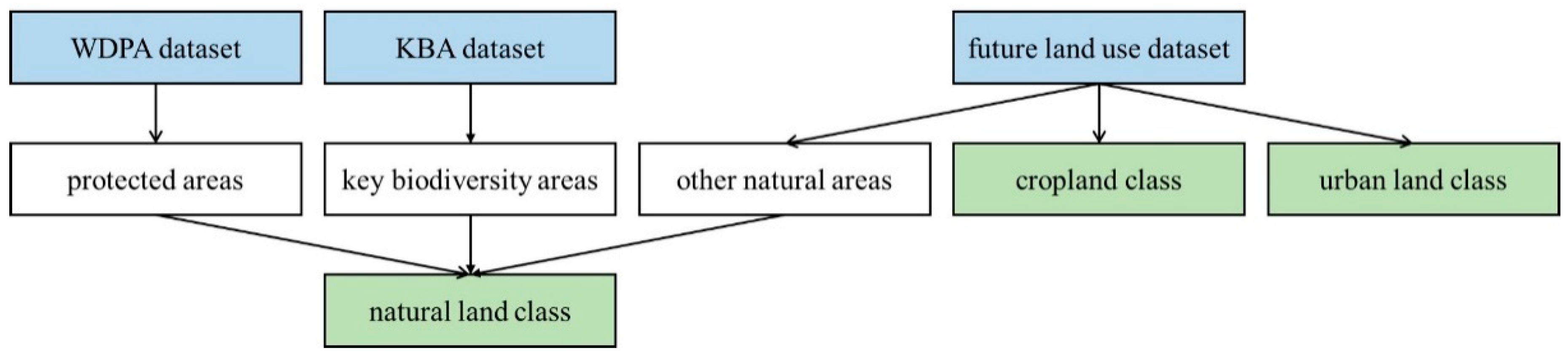
We define three types of land classes, that is, natural land class, cropland class and urban land class, and calculate the area of each land class within each 8.4 km pixel (Figure 1).

Natural land class includes protected areas, Key Biodiversity Areas (KBAs) and other natural areas (i.e., forest, grassland, bare land and snow/ice). To identify protected areas, we use World Database on Protected Areas (WDPA) obtained in September 2020. WDPA is the most comprehensive global database on Protected Areas (PAs), including various types of protected areas defined by the International Union for Conservation of Nature (IUCN) and Convention on Biological Diversity (CBD) [22]. We collect data on KBAs, which are sites contributing significantly to the global persistence of biodiversity in terrestrial, inland water, and marine environments [23]. We resample PAs and KBAs to 8.4 km by nearest neighbor interpolation and assume that there is no cropland class or urban land class in protected areas.

We identify cropland class and urban land class on the basis of future land use. Impacts from different shared socioeconomic pathways (SSPs) and the representative concentration pathways (RCPs) [24] are indispensable for future land use. Considering urban land demand and subsequent expansion, future distribution of water, forest, grassland, bare land, cropland, urban land and snow/ice is projected under 8 scenarios, that is SSP1-RCP1.9, SSP1-RCP2.6, SSP2-RCP4.5, SSP3-RCP7.0, SSP4-RCP3.4, SSP4-RCP6.0, SSP5-RCP3.4 and SSP5-RCP8.5. This dataset provides land use projections at global scale from 2020 to 2100 with a spatial resolution of 1 km. Calculating the area of cropland class for each 8.4 km pixel is a three-step process. The pixel counting method we use requires that the large pixels contain an integer number of small pixels. Hence, we have to calculate the cropland area percentage at an 8 km resolution (each 8 km pixel contains 64 1 km pixels) instead of 8.4 km resolution and then resample the intermediate result to get cropland area within 8.4 km pixel. First, to obtain cropland area within 8 km pixel, we count the number of 1 km cropland pixels included by each 8 km pixel and then multiply the number by the actual area of each cropland pixel (that is, 1 km × 1 km). Subsequent, cropland area percentage with a spatial resolution of 8 km is calculated from cropland area within 8 km pixel and total area of an 8 km pixel. Third, the percentage dataset is resampled to 8.4 km by bilinear interpolation and cropland area within 8.4 km pixel can be calculated under Eckert IV’s equal-area projection. The calculation of the area of urban land class is the same as that of the cropland class. After removing the area of cropland class and urban land class, the remaining area in a pixel is the area of other natural lands.

2.2. Step 2: Defining Pixel Types

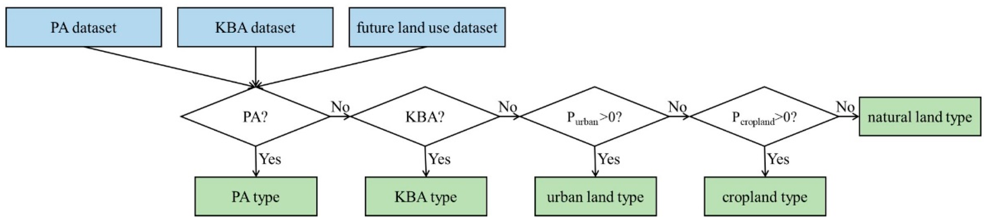
According to land classes obtained in step 1, we further define five types, which are as follows [21]: (1) PA; (2) KBA; (3) natural land (i.e., forest, grassland, bare land and snow/ice); (4) cropland; (5) urban land. We focus on the terrestrial area and exclude water bodies. Antarctica and Greenland are not included in this study.

The process of defining pixel types is shown in Figure 2. First, pixels occupied by PA land class (we assume PA/KBA land class occupying the entire pixel in step 1) are defined as PA type. Second, for the remaining pixels, the ones occupied by KBA land class are defined as KBA type. Third, we regard pixels whose area percentage of urban land class is greater than 0 as urban land type. Fourth, pixels with cropland class distribution but without urban land class distribution are defined as cropland type. At last, the pixels which do not belong to the above four types are regarded as natural land type.

2.3. Step 3: Calculating Calories of Pixels

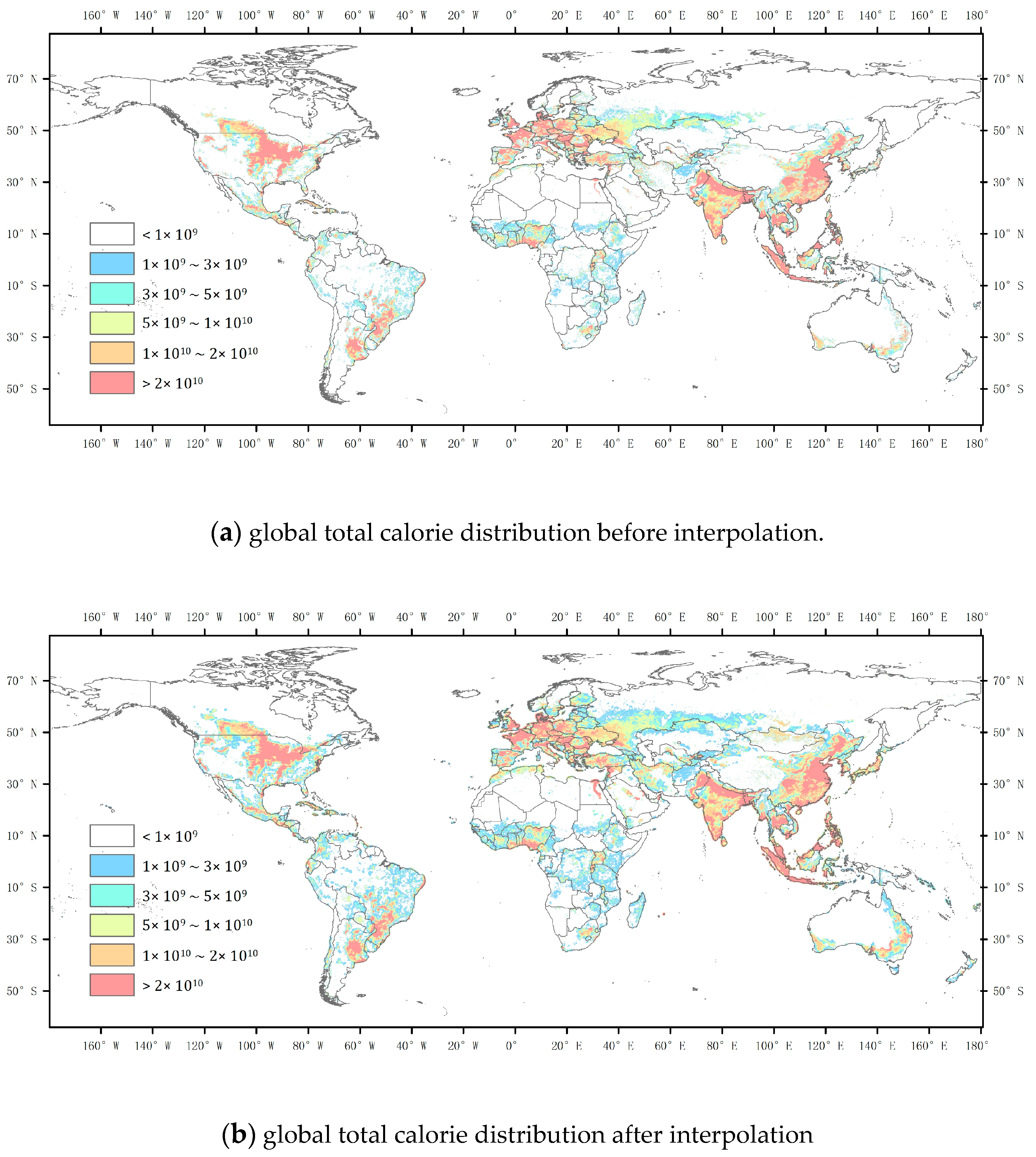
We then calculate calories provided by each pixel as calorie indicates agricultural productivity, which would be considered in identifying conservation areas in the next step. The calorie dataset uses mapped global patterns of production and allocation of 41 major crops, which provides more than 90% of global calories [25]. This dataset integrates global census data and satellite images from 1997 to 2003, with a spatial resolution of 5 arc-minutes (we resample the dataset to 8.4 km-resolution by bilinear interpolation, to match other datasets). Calculation of future calorie distribution based on the projected land use dataset faces the problem of high similarity with and dependency on land use and the reliability of the prediction results is hard to be guaranteed. Thus, we use global total calories in 2000, which are produced for all types of allocations (human directly consumption, animal feed, biofuels, and other non-food products), and interpolate the dataset to be consistent with cropland distribution.

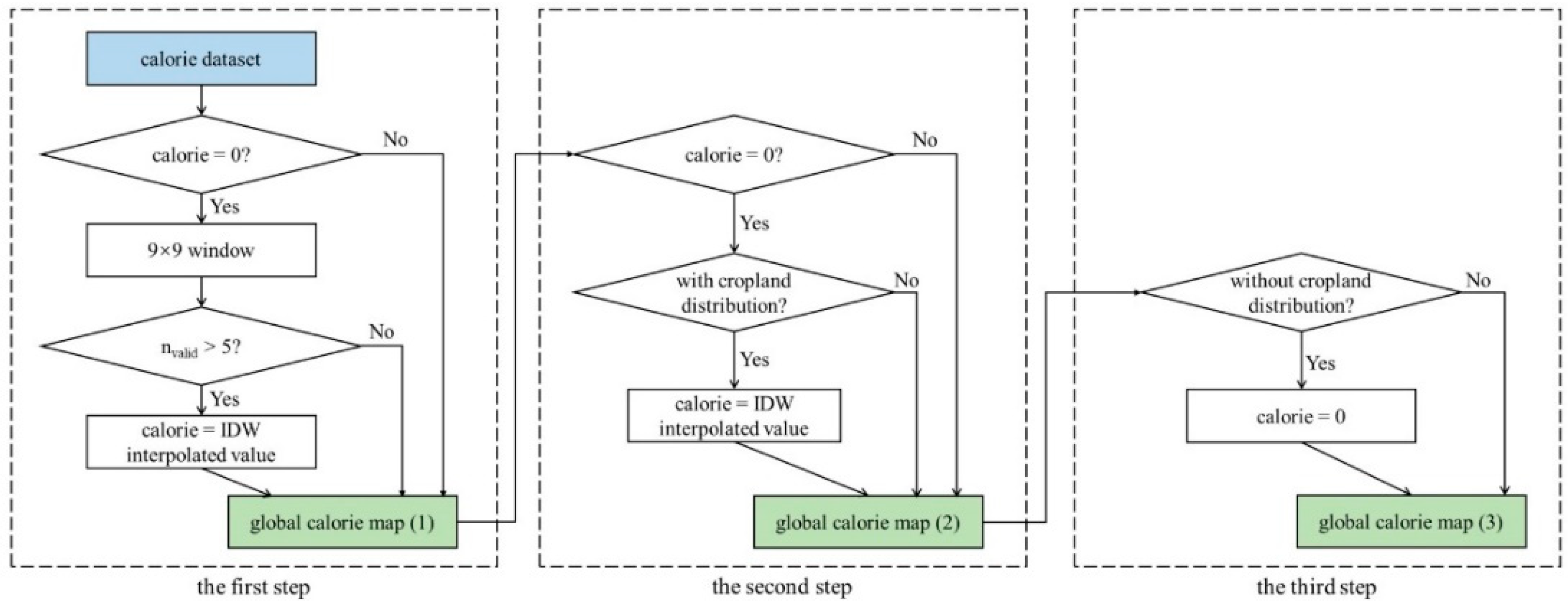
Calorie and cropland area datasets are multi-resource datasets, leading to data inconsistency to some extent. Calculating calories of pixels is a three-step process, including using a 9 × 9 window to interpolate, using the global calorie map obtained from the first step to interpolate and ensuring consistency between cropland distribution and interpolated calorie distribution (Figure 3).

Some pixels with cropland distribution lack distribution of calorie and interpolation is indispensable for calorie dataset. We make sure that each pixel with cropland distribution provides calories through the first step and the second step. In the first step, we regard pixels without calorie as target pixels and for each target pixel, we identify a 9 × 9 window centered on it. Pixels with calorie distribution are regarded as valid pixels for interpolation in the window. If there are more than 5 valid pixels in the window, we apply Inverse Distance Weight (IDW) interpolation to predict the calorie value of the target pixel based on all valid pixels in the window. After the first step, there are still some pixels keeping calorie value as zero due to the absence of enough valid pixels in the 9 × 9 window. In the second step, pixels whose calorie value remains zero after the first step and the percentage of cropland area is greater than zero are target pixels. We take the global calorie map obtained from the first step as a window and use all valid pixels in the global calorie map to apply IDW interpolation. After the second step, we make sure that pixels with cropland distribution provide calories simultaneously. Besides, the second step is conducted, respectively for 2030 and 2050 under each future scenario. Through the third step, we solve the problem that some pixels lack cropland distribution but have calorie distribution, owing to inconsistency among datasets or the first step of calorie interpolation. Thus, in the third step, we set the calorie value of these pixels as zero and make sure calorie distribution and cropland distribution coincide. The comparison of global total calories before and after interpolation is analyzed in Figure 4 and Supplementary Table S1.

2.4. Step 4: Identifying Conservation Areas According to Ranking of Pixels and Land Classes

In this study, we set two targets: conserving 30% of Earth by 2030 and conserving 50% of Earth by 2050. For each target, analyses are conducted based on six combinations of three spatial scales and two approaches (Figure 5). At the global scale, 30% or 50% of the global terrestrial area is conserved; at biome scale, 30% or 50% of each biome’s terrestrial area is conserved; at the national scale, 30% or 50% of each country’s terrestrial area is conserved. When calculating the percentage of land given back to nature in order to conserve 30% or 50% of Earth, we take the two types into account. One is retaining natural lands, such as protected areas and key biodiversity areas, which are the first to be conserved owing to their high value of biodiversity. The other is restoring land currently under human pressure like cropland and urban areas.

Under the nature-only approach, all crop production in conserved pixels is converted to conservation. Thus, an entire pixel rather than land classes within the pixel is conserved. First of all, pixels of different types are conserved in the following ranking: (1) pixels of PA; (2) pixels of KBA type; (3) pixels of natural land type; (4) pixels of cropland type; (5) pixels of urban land type. There are several reasons for this ranking: many PAs and KBA are already under protection and are thus easy to be conserved first; compared to conserving cropland or urban land, conserving natural land has fewer impacts on humans and is much easier; cropland losses should be minimized for food security; urban land is the most difficult to give back to nature. Furthermore, pixels of the same type are conserved in the ascending ranking of calories considering food security. The fewer calories the pixels provide, the earlier they are conserved or restored.

Under the shared approach, cropland and conservation could coexist in any possible spatial layout within a pixel. Thus, land class is the smallest unit of conservation of restoration. In the analysis, the ranking of conservation and restoration is as follows considering pixel types and land classes: (1) pixels of PA type; (2) pixels of KBA type; (3) pixels of natural land type; (4) natural land classes located in pixels of cropland type; (5) cropland classes located in pixels of cropland type; (6) natural land classes located in pixels of urban land type; (7) cropland classes located in pixels of urban land type; (8) urban land classes located in pixels of urban land type. Furthermore, within each of the above eight types, pixels or land classes are conserved and restored in the ascending ranking of calories.

2.5. Step 5: Identifying Potential Cropland Losses

With conservation areas increasing, we identify cropland losses and their location at different scales and under different approaches, using future land use which is projected under 8 different scenarios.

For the global, each biome and typical countries, the relationship curve between the percentage of cropland losses and the percentage of land given back is unfolded. Future land use under different scenarios affects the mean and ranges of cropland losses. Through this relationship curve, we can identify the specific percentage of land given back at which cropland losses start to occur. That means the extreme limit of conserving without any cropland loss.

In order to testify the feasibility of the bold conservation targets, we calculate the percentage of cropland losses when conserving 30% or 50% of the globe, each biome and each country by 2030/2050. Especially, we analyze countries’ cropland losses at different spatial scales to identify the countries suffering from severe conflicts between nature conservation and food security.

3. Results

3.1. Potential Cropland Losses at the Global Scale

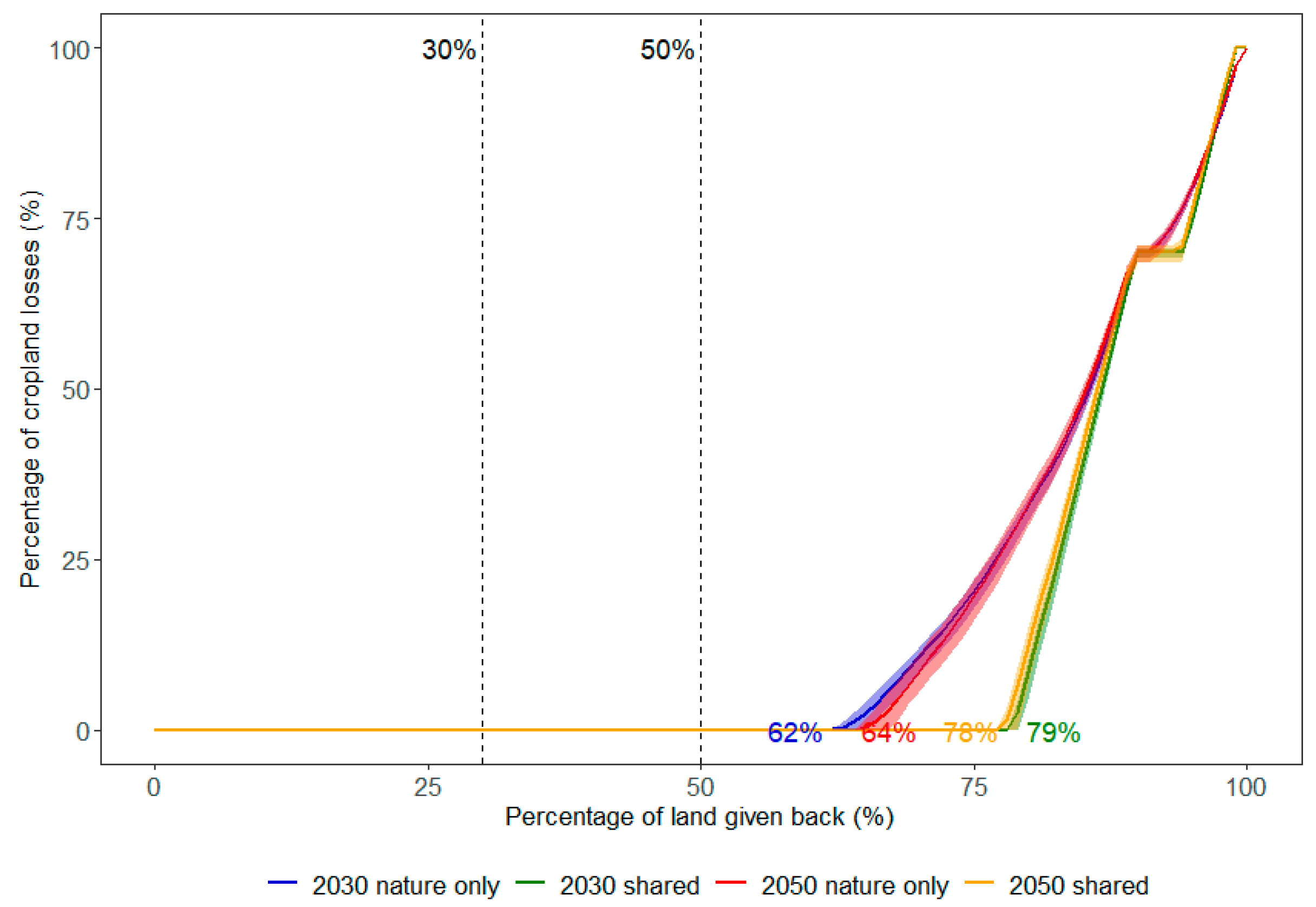
According to our analysis, at the global scale, conserving 30% land in 2030 and 50% land in 2050 globally will not cause cropland losses over the world (Figure 6). As shown in the figure, the nature-only approach will cause cropland losses when the percentage of land given back reaches 62% in 2030 and 64% in 2050 while the counterpart of the shared approach is 79% in 2030 and 78% in 2050. Under the shared approach, cropland begins to suffer loss at a smaller percentage of land given back in 2050 than in 2030, since cropland is abandoned earlier than rapidly expanding urban areas so as to maintain human life. This indicates the feasibility of achieving bold conservation targets without causing cropland loss, which is inspiring for both biodiversity conservation and food security, while more factors should be considered to predict the complicated impacts in a more comprehensive way.

3.2. Potential Cropland Losses at the Biome Scale

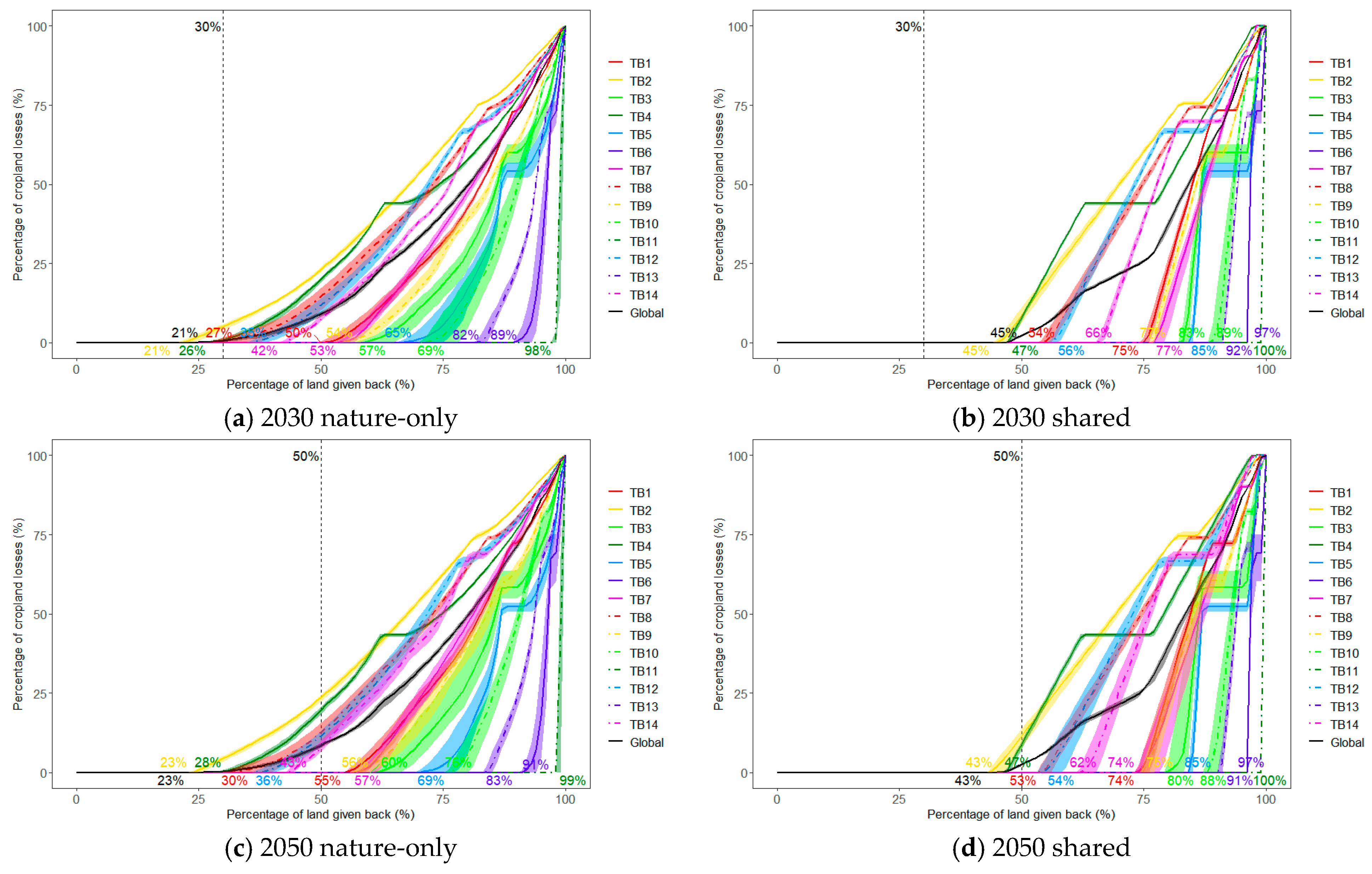
At the biome scale, we allocate half of each terrestrial biome (TB) back to nature so as to leave half of the Earth for nature conservation. There are 14 different TBs which involve 876 terrestrial ecoregions over the world, facilitating representation analyses [26]. The 14 TBs include Tropical and Subtropical Moist Broadleaf Forests (referred to as TB1), Tropical and Subtropical Dry Broadleaf Forests (TB2), Tropical and Subtropical Coniferous Forests (TB3), Temperate Broadleaf and Mixed Forests (TB4), Temperate Conifer Forests (TB5), Boreal Forest/Taiga (TB6), Tropical and Subtropical Grasslands, Savannas and Shrublands (TB7), Temperate Grasslands, Savannas and Shrublands (TB8), Flooded Grasslands and Savannas (TB9), Montane Grasslands and Savannas (TB10), Tundra (TB11), Mediterranean Forests, Woodlands and Scrub (TB12), Deserts and Xeric Shrublands (TB13) and Mangroves (TB14). Under the nature-only approach in 2030, only 0.64% of cropland is abandoned over the world and there are few TBs suffered cropland losses due to 30% conserved land, including TB2 (Tropical and Subtropical Dry Broadleaf Forests) with 5.18%, TB4 (Temperate Broadleaf and Mixed Forests) with 0.97% and TB8 (Temperate Grasslands, Savannas and Shrublands) with 0.46%. Under the shared approach in 2030, the globe and all TBs are free of cropland losses when 30% of the terrestrial area is given back to nature. Only when the percentage of conserved land reaches 45% do the globe and TB2 begin to lose cropland. The other TBs bear losses of cropland even later. Under the nature-only approach in 2050, the percentages of abandoned cropland are 8.54%, 23.71%, 19.66%, 12.68%, 11.53% and 8.01% for the globe, TB2, TB4, TB8, TB12 (Mediterranean Forests, Woodlands and Scrub) and TB14 (Mangroves), respectively. Other TBs are capable of having all cropland kept. Under the shared approach in 2050, only TB2 and TB4 abandon 11.47% and 8.83% of cropland, respectively, occupying 2.59% of global cropland.

The above analysis shows the huge difference across biomes (Figure 7). TB2, TB4 and TB8 are mostly vulnerable biomes, which start to incur cropland losses when 30% and 50% of the land is conserved under the nature-only and shared approaches. TB6 (Boreal Forest/Taiga) and TB13 (Deserts and Xeric Shrublands) only lose cropland when approximately 90% of land is given back. TB11 (Tundra) is even more robust and faces cropland losses only when more than 98% of the terrestrial area is conserved, where cropland is much less than other biomes. The huge differences across biomes may be caused by many factors including the percentage of cropland, the land use land cover types. The results indicate that the difference between biomes should be carefully considered when conserving 30% or 50% of the Earth.

3.3. Potential Cropland Losses at the Country Scale

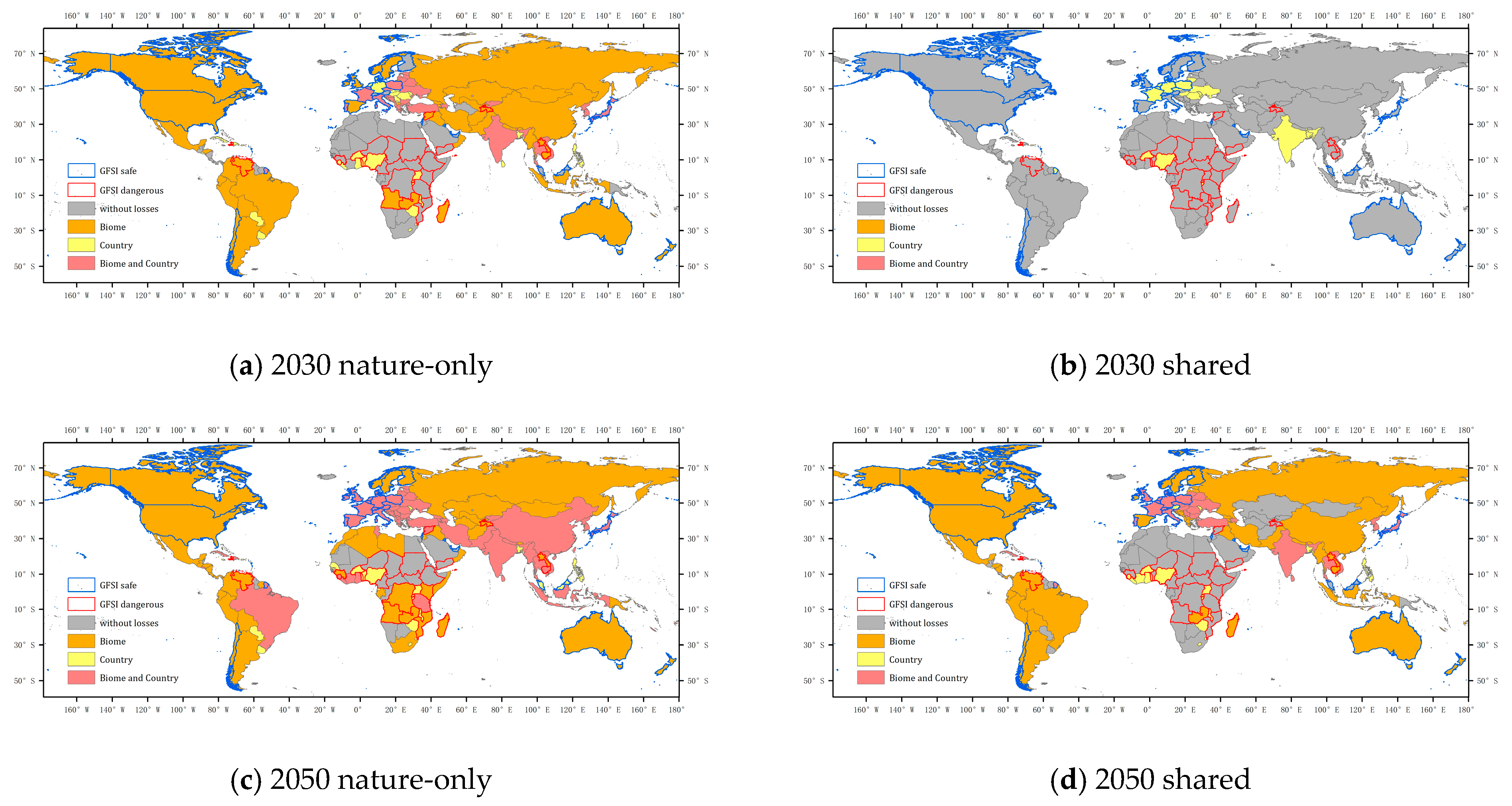
At the national scale, we simulate its cropland losses when achieving bold conservation targets for each country. As no predicted cropland losses occur at a global scale, countries could be classified into three types (Figure 8), including countries suffering from cropland losses only at biome scale, countries suffering from cropland losses only at the national scale, and countries suffer from cropland losses at both biome and the national scales. We introduce the 2019 Global Food Security Index (GFSI) to consider countries’ different conditions of food security. This index ranks the food security of 113 countries comprehensively, based on affordability, availability and quality [27].

Whether a country could fulfill Half-Earth plan and simultaneously avoid cropland losses is analyzed at different scales (Figure 8). Under the nature-only approach in 2030, most African countries are free of cropland losses at all three scales, including some countries with higher food security concerns according to the GFSI, like Ethiopia, Kenya and Tanzania. Under the shared approach in 2030, no countries have to face the dilemma between abandoning cropland and pursuing Half-Earth at biome scale, suggesting the target of conserving 30% of global terrestrial area does little harm to cropland over the world. Under the nature-only approach in 2050, the global situations are more pessimistic than 2030. Compared with 2030, the number of countries without cropland losses at all three scales decreases obviously; many countries have switched from abandoning cropland at only biome scale to abandoning cropland at both biome and the national scale in 2050, like China, Pakistan, Iran and Brazil. Most countries in Europe and Asia are challenged by cropland losses at two scales, even including some GFSI safe countries such as Britain, France, Germany, Switzerland and Austria. While under the shared approach in 2050, the situations are better than those under the nature-only approach in 2050. Many countries shoulder no cropland losses at all three scales, most of which are located in Africa, Central Asia and Western Asia.

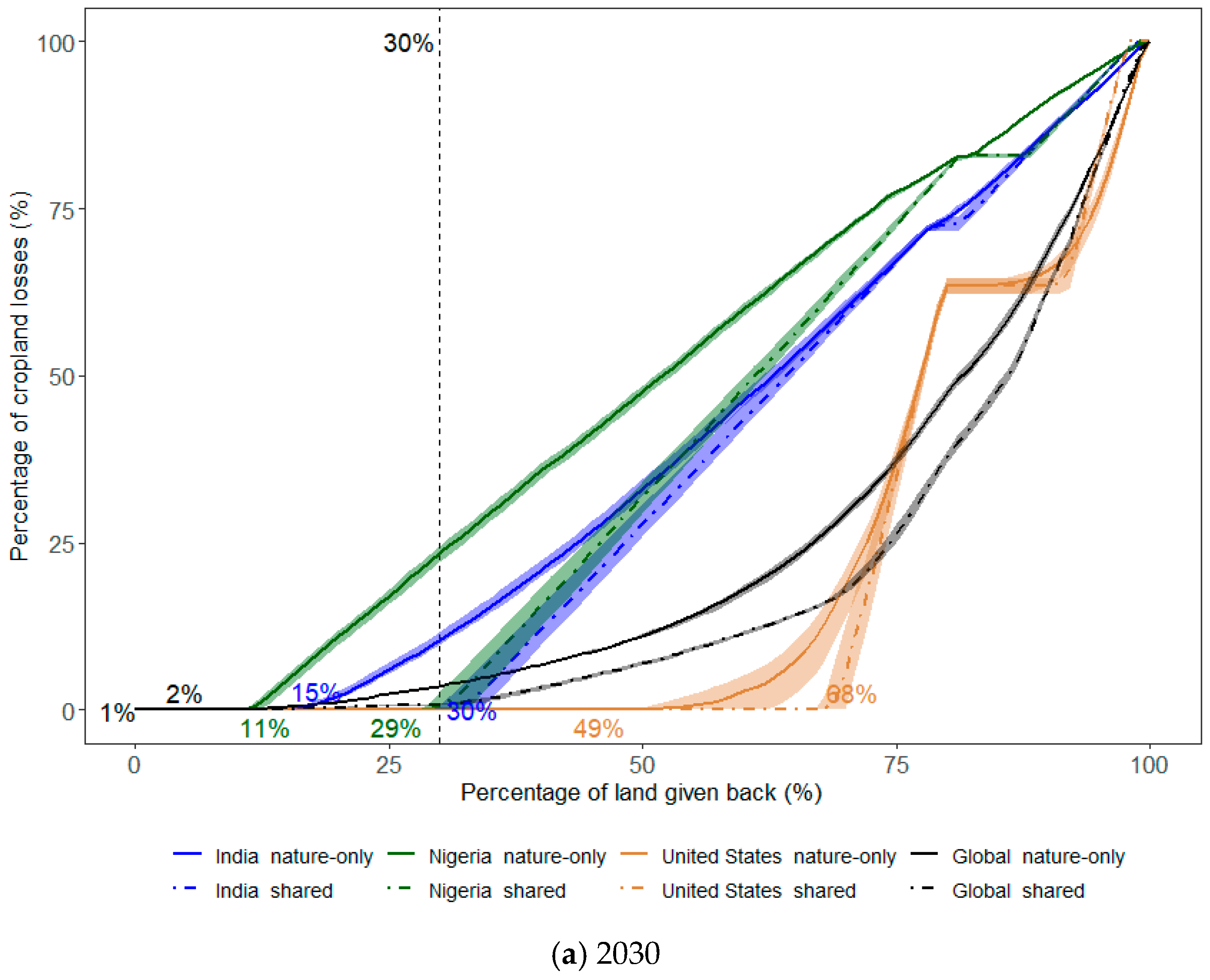
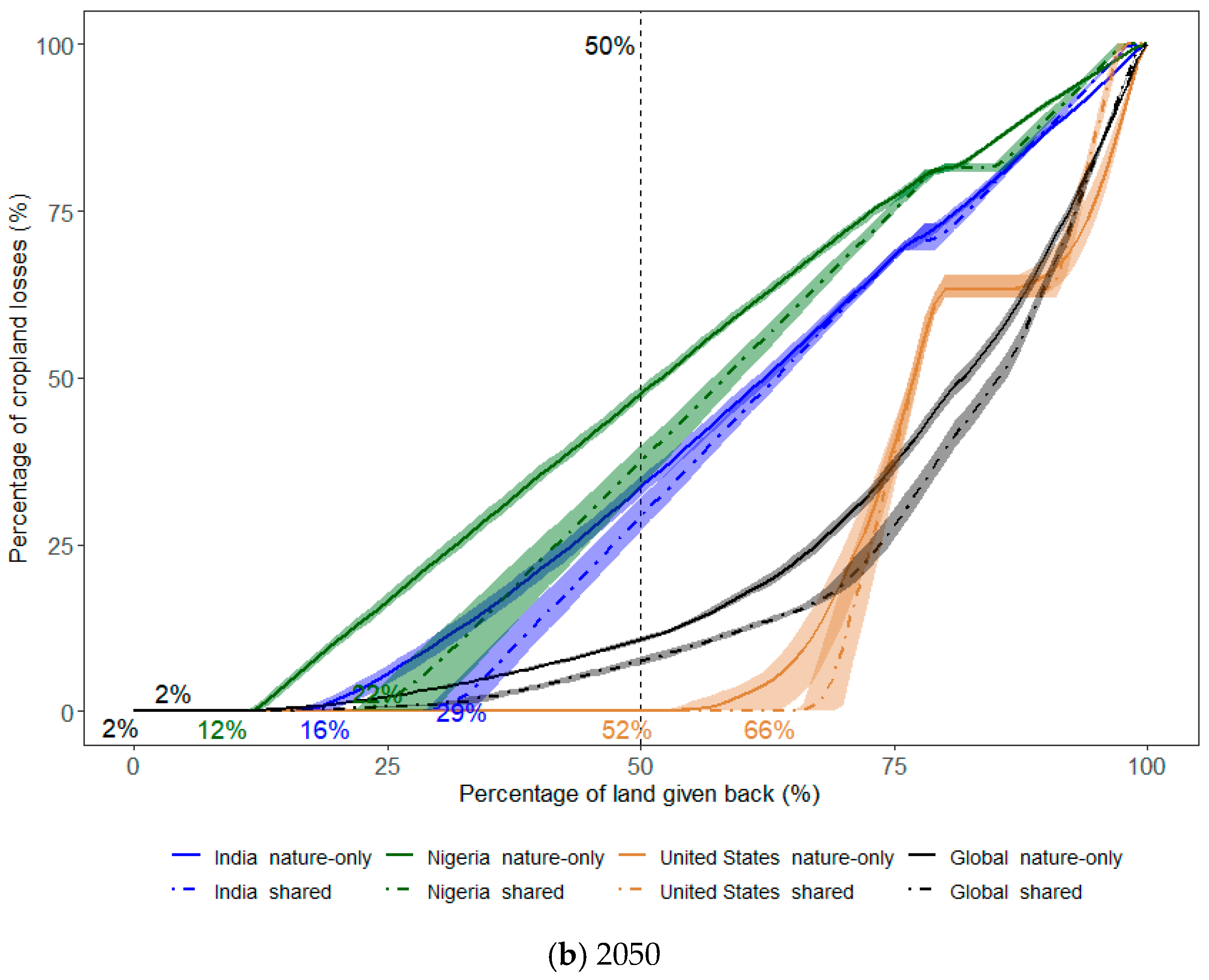
The United States, Nigeria and India are regarded as typical countries, respectively for the three types. Under at least three scenarios (there are four altogether including nature-only approach and shared approach in 2030/2050), United States abandons cropland only at biome scale, Nigeria abandons cropland only at the national scale and India abandons cropland at both biome and the national scale. Besides, these three countries have the largest arable land area of all countries in their respective types, according to FAOSTAT (The Food and Agriculture Organization Corporate Statistical Database). Thus, these countries could typically reflect impacts of achieving bold conservation targets on cropland for countries of different types (Figure 9). As shown in the figure, the United States begins to abandon cropland when more than half of its terrestrial land is conserved while India and Nigeria face cropland losses a lot earlier. When the percentage of land given back arrives at approximately 75%, for India and United States, cropland losses under the nature-only approach and shared approach are very close. By contrast, for Nigeria and the globe, there are more obvious differences between the cropland losses due to the nature-only approach and the shared approach. At the national scale, it is predicted that the nature-only approach demands 3.58% and 10.73% of global cropland in 2030 and 2050 for the Half-Earth plan. In comparison, under the shared approach, 0.77% and 7.55% of cropland are predicted to be abandoned in 2030 and 2050. The counterparts are 10.46%, 33.63%, 0.14% and 29.32% for India, 23.36%, 47.58%, 0.66% and 37.59% for Nigeria, 0%, 0%, 0% and 0% for United States.

3.4. Potential Area Percentage of Global Conserved Land Uses

For each land use, we summarize the percentage of its global conserved area to global terrestrial area at three spatial scales, respectively for 2030 nature-only (

Table 1. 2030 nature-only: percentage of conserved area to global terrestrial area.

	Global	Biome	Country
Pixels of PA type	13.88%	13.88%	13.52%
Pixels of KBA type	4.48%	4.42%	3.89%
Pixels of natural land type	12.14%	12.09%	12.51%
Pixels of cropland type	0.00%	0.10%	0.57%
Pixels of urban land type	0.00%	0.00%	0.01%
Total	30.50%	30.50%	30.49%

), 2030 shared (

Table 2. 2030 shared: percentage of conserved area to global terrestrial area.

	Global	Biome	Country
Pixels of PA type	13.88%	13.88%	13.60%
Pixels of KBA type	4.48%	4.43%	4.00%
Pixels of natural land type	12.14%	11.68%	11.58%
Natural land classes located in pixels of cropland type	0.00%	0.50%	1.13%
Cropland classes located in pixels of cropland type	0.00%	0.00%	0.12%
Natural land classes located in pixels of urban land type	0.00%	0.00%	0.06%
Cropland classes located in pixels of urban land type	0.00%	0.00%	0.00%
Urban land classes located in pixels of urban land type	0.00%	0.00%	0.01%
Total	30.50%	30.50%	30.49%

), 2050 nature-only (

Table 3. 2050 nature-only: percentage of conserved area to global terrestrial area.

	Global	Biome	Country
Pixels of PA type	13.88%	13.88%	13.88%
Pixels of KBA type	4.48%	4.48%	4.47%
Pixels of natural land type	32.14%	30.72%	30.34%
Pixels of cropland type	0.00%	1.42%	1.79%
Pixels of urban land type	0.00%	0.00%	0.02%
Total	50.50%	50.50%	50.49%

) and 2050 shared (

Table 4. 2050 shared: percentage of conserved area to global terrestrial area.

	Global	Biome	Country
Pixels of PA type	13.88%	13.88%	13.88%
Pixels of KBA type	4.48%	4.48%	4.47%
Pixels of natural land type	32.14%	28.13%	28.73%
Natural land classes located in pixels of cropland type	0.00%	3.58%	1.90%
Cropland classes located in pixels of cropland type	0.00%	0.43%	1.17%
Natural land classes located in pixels of urban land type	0.00%	0.00%	0.25%
Cropland classes located in pixels of urban land type	0.00%	0.00%	0.00%
Urban land classes located in pixels of urban land type	0.00%	0.00%	0.09%
Total	50.50%	50.50%	50.49%

). Since the unit of land conservation is pixel/land class, the total percentage of conserved area to the global terrestrial area slightly exceeds 30%/50% rather than being exactly 30%/50%.

According to the ranking rule of conservation has been noted in 2.4, the area already under protection (PA and KBA) and most other natural areas are conserved earlier than cropland and occupy a large percentage of potential global conserved area. That explains why global cropland losses are bearable while achieving bold conservation targets.

4. Discussion

In this study, we have identified potential cropland losses when conserving 30% and 50% Earth with different approaches and spatial scales. The lessons learned here are the importance of approaches and spatial scales which have been selected in planning effective conservation landscapes. As different approaches and spatial scales will cause huge differences, so they should be carefully chosen in spatial planning to achieve bold conservation targets.

Our analysis contributes to the literature by incorporating data on future land use and land cover, and simulating multiple scenarios to obtain a more comprehensive understanding on the effects of achieving bold conservation targets on cropland losses. The above findings could be useful for policymakers, especially in the context of creating and implementing the post-2020 global biodiversity framework. However, these findings largely rely on the methods and assumptions used in the study, so further research is required to assess the impacts of achieving bold conservation targets in a more comprehensive way. The following points need to be clarified to illustrate the limitations and future research directions based on this study.

First, although bold conservation target increases many interests, the validity, feasibility, and outcomes of bold conservation targets, especially the half Earth proposal, is still under discussion. On one hand, it is still a challenge to science that how much land should be set for biodiversity conservation at the global scale in order to bend the curve of biodiversity loss. On the other hand, the half Earth proposal may cause negative social and economic consequences, for example, Schleicher et al. (2019) [11] points out that protecting half of the planet could directly affect over one billion people. Therefore, the analysis in this study is a what-if modelling under multiple scenarios based on certain assumptions, and thus more factors should be further considered in order to assess the comprehensive effects of achieving bold conservation targets.

Second, our results are different from previous studies and thus further comparison and analyses are required. Mehrabi et al. (2018) concluded that “globally, 15–31% of cropland, 10–45% of pasture land, 23–25% of non-food calories and 3–29% of food calories from crops could be lost if half of Earth’s terrestrial ecoregions were given back to nature”. Although our study references the study design and method of this previous study, we get different results. This may be caused because our study using different land use datasets, not considering pasture land, focusing on total calories instead of distinguishing food and non-food calorie, conserving all land classes located in pixels of urban types after conserving cropland.

Third, trade-offs between biodiversity conservation and cropland production need to be analyzed at the local scale considering the huge spatial and temporal heterogeneity across global landscapes. As a global analysis, we simulate possible cropland losses under different spatial scales and approaches. While this kind of analysis may be very different from the reality as conservation actions are designed by multiple stakeholders in the real world. Therefore, the analysis in this study could only serve as a reference for policymaking and more complicated factors need to be taken into consideration at the local scale. In addition, while shared and nature-only strategies cause different results in general, there is no one-size-fits-all approach, and they may play different roles in different regions considering the huge spatial and temporal heterogeneity. To further guide policies, it is also crucial to assess the potential biodiversity values of rewilding cropland, in order to achieve a win-win situation for biodiversity conservation and agricultural production.

5. Conclusions

In conclusion, based on our analysis (which may be one way in achieving the half Earth ambition), it is possible to succeed while having minimum cropland losses at the global scale. At biome scale, 0.64% and 8.54% cropland are abandoned globally in 2030 and 2050 under the nature-only approach while by contrast, the shared approach substantially reduces the number of countries confronted by cropland losses, demanding only 0% and 2.59% of global cropland losses in 2030 and 2050. At the national scale, the nature-only approach causes losses of 3.58% and 10.73% of global cropland in 2030 and 2050 while a shared approach requires 0.77% and 7.55% cropland losses in 2030 and 2050. Hence, trade-offs under the shared approach are affordable for global food security but may still pose a grave threat to GFSI dangerous countries like Burkina Faso and Nigeria. Overall, under the shared approach, most countries bear cropland losses only at biome scale or even require no cropland losses. This indicates that bold conservation targets are achievable to a certain degree, especially when adopting the shared approach. While it still requires a careful balance between biodiversity conservation and agricultural production, and detailed strategies are required for those vulnerable countries. While acknowledging complex social, economic and political factors that may be at play to achieve the goal for biodiversity conservation, we call on the governments to adopt ambitious targets (protecting at least 30% by 2030) at the UN Biodiversity Conference.

References

- Balmford, A.; Amano, T.; Bartlett, H.; Chadwick, D.; Collins, A.; Edwards, D.; Field, R.; Garnsworthy, P.; Green, R.; Smith, P.; et al. The environmental costs and benefits of high-yield farming. Nat. Sustain. 2018, 1, 477–485. [Google Scholar] [CrossRef]
- Butchart, S.H.M.; Walpole, M.; Collen, B.; van Strien, A.; Scharlemann, J.P.W.; Almond, R.E.A.; Baillie, J.E.M.; Bomhard, B.; Brown, C.; Bruno, J.; et al. Global Biodiversity: Indicators of Recent Declines. Science 2010, 328, 1164–1168. [Google Scholar] [CrossRef] [PubMed]
- Newbold, T.; Hudson, L.N.; Arnell, A.P.; Contu, S.; De Palma, A.; Ferrier, S.; Hill, S.L.L.; Hoskins, A.J.; Lysenko, I.; Phillips, H.R.P.; et al. Has land use pushed terrestrial biodiversity beyond the planetary boundary? A global assessment. Science 2016, 353, 288–291. [Google Scholar] [CrossRef]
- Jones, K.R.; Venter, O.; Fuller, R.A.; Allan, J.R.; Maxwell, S.L.; Negret, P.J.; Watson, J.E.M. One-third of global protected land is under intense human pressure. Science 2018, 360, 788–791. [Google Scholar] [CrossRef] [Green Version]
- Mace, G.M.; Barrett, M.; Burgess, N.D.; Cornell, S.E.; Freeman, R.; Grooten, M.; Purvis, A. Aiming higher to bend the curve of biodiversity loss. Nat. Sustain. 2018, 1, 448–451. [Google Scholar] [CrossRef]
- Yang, R.; Cao, Y.; Hou, S.; Peng, Q.; Wang, X.; Wang, F.; Tseng, T.; Yu, L.; Carver, S.; Convery, I.; et al. Cost-effective priorities for the expansion of global terrestrial protected areas: Setting post-2020 global and national targets. Sci. Adv. 2020, 6, eabc3436. [Google Scholar] [CrossRef] [PubMed]
- Locke, H. Nature needs half: A necessary and hopeful new agenda for protected areas. Nat. N. S. W. 2014, 58, 7–17. [Google Scholar] [CrossRef]
- Wilson, E.O. Half-Earth, reprint ed.; Liveright: New York, NY, USA, 2017. [Google Scholar]
- Leclère, D.; Obersteiner, M.; Barrett, M.; Butchart, S.H.M.; Chaudhary, A.; De Palma, A.; DeClerck, F.A.J.; Di Marco, M.; Doelman, J.C.; Dürauer, M.; et al. Bending the curve of terrestrial biodiversity needs an integrated strategy. Nature 2020, 585, 551–556. [Google Scholar] [CrossRef] [PubMed]
- Dinerstein, E.; Olson, D.; Joshi, A.; Vynne, C.; Burgess, N.D.; Wikramanayake, E.; Hahn, N.; Palminteri, S.; Hedao, P.; Noss, R.; et al. An Ecoregion-Based Approach to Protecting Half the Terrestrial Realm. Bioscience 2017, 67, 534–545. [Google Scholar] [CrossRef] [PubMed]
- Schleicher, J.; Zaehringer, J.G.; Fastré, C.; Vira, B.; Visconti, P.; Sandbrook, C. Protecting half of the planet could directly affect over one billion people. Nat. Sustain. 2019, 2, 1094–1096. [Google Scholar] [CrossRef]
- Fischer, J.; Abson, D.J.; Bergsten, A.; French Collier, N.; Dorresteijn, I.; Hanspach, J.; Hylander, K.; Schultner, J.; Senbeta, F. Reframing the Food–Biodiversity Challenge. Trends Ecol. Evol. 2017, 32, 335–345. [Google Scholar] [CrossRef]
- Molotoks, A.; Kuhnert, M.; Dawson, T.; Smith, P. Global Hotspots of Conflict Risk between Food Security and Biodiversity Conservation. Land 2017, 6, 67. [Google Scholar] [CrossRef] [Green Version]
- Riggio, J.; Baillie, J.E.M.; Brumby, S.; Ellis, E.; Kennedy, C.M.; Oakleaf, J.R.; Tait, A.; Tepe, T.; Theobald, D.M.; Venter, O.; et al. Global human influence maps reveal clear opportunities in conserving Earth’s remaining intact terrestrial ecosystems. Glob. Chang. Biol. 2020, 26, 4344–4356. [Google Scholar] [CrossRef]
- Navarro, L.M.; Pereira, H.M. Rewilding Abandoned Landscapes in Europe. Ecosystems 2012, 15, 900–912. [Google Scholar] [CrossRef] [Green Version]
- Estel, S.; Kuemmerle, T.; Alcántara, C.; Levers, C.; Prishchepov, A.; Hostert, P. Mapping farmland abandonment and recultivation across Europe using MODIS NDVI time series. Remote Sens. Environ. 2015, 163, 312–325. [Google Scholar] [CrossRef]
- Queiroz, C.; Beilin, R.; Folke, C.; Lindborg, R. Farmland abandonment: Threat or opportunity for biodiversity conservation? A global review. Front. Ecol. Environ. 2014, 12, 288–296. [Google Scholar] [CrossRef]
- Ceaușu, S.; Hofmann, M.; Navarro, L.M.; Carver, S.; Verburg, P.H.; Pereira, H.M. Mapping opportunities and challenges for rewilding in Europe. Conserv. Biol. 2015, 29, 1017–1027. [Google Scholar] [CrossRef] [PubMed] [Green Version]
- Li, S.; Li, X. Global understanding of farmland abandonment: A review and prospects. J. Geogr. Sci. 2017, 27, 1123–1150. [Google Scholar] [CrossRef]
- Dinerstein, E.; Vynne, C.; Sala, E.; Joshi, A.R.; Fernando, S.; Lovejoy, T.E.; Mayorga, J.; Olson, D.; Asner, G.P.; Baillie, J.E.M.; et al. A Global Deal For Nature: Guiding principles, milestones, and targets. Sci. Adv. 2019, 5, eaaw2869. [Google Scholar] [CrossRef] [Green Version]
- Mehrabi, Z.; Ellis, E.C.; Ramankutty, N. The challenge of feeding the world while conserving half the planet. Nat. Sustain. 2018, 1, 409–412. [Google Scholar] [CrossRef] [Green Version]
- UNEP-WCMC; IUCN. World Database on Protected Areas. Available online: https://www.protectedplanet.net/ (accessed on 9 September 2020).
- BirdLife International. World Database of Key Biodiversity Areas. Available online: http://www.keybiodiversityareas.org/ (accessed on 28 March 2020).
- Chen, G.; Li, X.; Liu, X.; Chen, Y.; Liang, X.; Leng, J.; Xu, X.; Liao, W.; Qiu, Y.A.; Wu, Q.; et al. Global projections of future urban land expansion under shared socioeconomic pathways. Nat. Commun. 2020, 11, 537. [Google Scholar] [CrossRef] [PubMed] [Green Version]
- Cassidy, E.S.; West, P.C.; Gerber, J.S.; Foley, J.A. Redefining agricultural yields: From tonnes to people nourished per hectare. Environ. Res. Lett. 2013, 8, 34015. [Google Scholar] [CrossRef]
- Olson, D.M.; Dinerstein, E.; Wikramanayake, E.D.; Burgess, N.D.; Powell, G.V.N.; Underwood, E.C.; D’Amico, J.A.; Itoua, I.; Strand, H.E.; Morrison, J.C.; et al. Terrestrial Ecoregions of the World: A New Map of Life on Earth. Bioscience 2001, 51, 933. [Google Scholar] [CrossRef]
- The Economist Intelligence Unit. Global Food Security Index 2019. Available online: http://foodsecurityindex.eiu.com/ (accessed on 5 August 2020).
Figure 1.
Flow chart of defining land classes. Blue represents input datasets. Green represents outputs in this step, which are land classes we define.
Figure 2.
Flow chart of defining pixel types. Blue represents input datasets. Green represents outputs in this step, that is, pixel types we define. Here, Purban represents area percentage of urban land class in a pixel while Pcropland represents area percentage of cropland class in a pixel.
Figure 3.
Flow chart of calculating calories of pixels. Blue represents input dataset. Green represents outputs in each step. Global calorie map (1) and global calorie map (2) are intermediate outputs to get global calorie map (3) which is useful in the next step. Here, nvalid represents the number of pixels calorie distribution in a 9 × 9 window.
Figure 4.
The comparison of global total calorie distribution before and after interpolation. According to
Supplementary Table S1, the sum of global total calorie under SSP4-RCP6.0 in 2030 is the largest and differs most from the sum of origin total calorie. Thus, we map interpolated calorie distribution under SSP4-RCP6.0 in 2030 to visualize the difference. Antarctica and Greenland are not included on the map.
Figure 5.
The six combinations of three spatial scales and two approaches in identifying conservation areas according to ranking of pixels and land classes.
Figure 6.
Predicted cropland losses at a global scale. The curve reflects the mean value of all 8 scenarios and the shadows show ranges of all scenarios. Percentage of cropland losses is the area percentage of global conserved cropland to global cropland. The specific percentage of land given back at which cropland begins to be abandoned is marked. Land given back and cropland losses are both shown in percentages.
Figure 7.
Cropland losses of all TBs and the globe at the biome scale. The figure shows the percentages of cropland abandoned within each TB and the whole globe as the terrestrial area given back to nature increasing. The curve reflects the mean value of all 8 scenarios and the shadows show ranges of all scenarios. The specific percentage of land given bank at which cropland begins to be abandoned is marked. Land given back and cropland losses are both shown in percentages.
Figure 8.
Countries’ conditions of fulfilling Half-Earth plan under different scales. Countries with GFSI in the top 25% are identified as GFSI safe and bordered with blue. Countries with GFSI in the bottom 25% are identified as GFSI dangerous and bordered with red. Countries filled with gray are free of cropland losses at all three scales. Orange, yellow and pink represent the scale, at which countries have to abandon cropland. Antarctica and Greenland are not included on the map.
Figure 9.
Cropland losses of typical countries and the globe at the national scale. The curve reflects the mean value of all 8 scenarios and the shadows show ranges of all scenarios. The specific percentage of land given bank at which cropland begins to be abandoned is marked. Land given back and cropland losses are both shown in percentages.