Article

A Simple GIS-Based Tool for the Detection of Landslide-Prone Zones on a Coastal Slope in Scotland

by
Alejandro Gonzalez-Ollauri
and
Slobodan B. Mickovski
*
The BEAM Research Centre, School of Computing, Engineering and Built Environment, Glasgow Caledonian University, Glasgow G4 0BA, UK
*
Author to whom correspondence should be addressed.
Land 2021, 10(7), 685; https://doi.org/10.3390/land10070685
Submission received: 17 May 2021 / Revised: 10 June 2021 / Accepted: 23 June 2021 / Published: 28 June 2021
(This article belongs to the Section Soil-Sediment-Water Systems)

Abstract

:
Effective landslide detection is crucial to mitigate the negative impacts derived from the occurrence of these natural hazards. Research on landslide detection methods has been extensively undertaken. However, simplified methods for landslide detection requiring a minimum amount of data inputs are still lacking. Simple approaches for landslide detection should be particularly interesting for geographical areas with limited information or resources availability. The aim of this paper is to present a refined, simple, GIS-based tool for the detection of landslide-prone and slope restoration zones. The tool only requires a digital elevation model (DEM) dataset as input, it is interoperable at multiple spatial scales, and it can be implemented on any GIS platform. The tool was applied on a coastal slope prone to instability, located in Scotland, in order to verify the functionality of the tool. The results indicated that the proposed tool is able to detect both shallow and deeper landslides satisfactorily, suggesting that the spatial combination of steep and potentially wet soil zones is effective for detecting areas prone to slope failure.

1. Introduction

Soil loss jeopardizes the integrity and function of the Earth’s ecosystems. Landslides, in particular, have been recognised as one of the main drivers of soil loss globally [1] with a severity and recurrence which is most likely to increase under the predicted scenarios of climate change due to the potential intensification of the hydrological cycle [2], which is linked to the occurrence of rainfall-induced landslides [3]. Landslides can be classified in accordance with scale, location of occurrence, cause, material (e.g., mud, soil, rock) and predominant type of movement (e.g., falls, topples, flows etc.; [4]). Landslide events often comprise more than one type of movement, so it is challenging to classify distinct types of landslides. All landslides are potential hazards, but most of them occur in remote areas away from densely populated urban areas (e.g., mountainous zones). However, when landslide hazards occur near human settlements, landslides can have devastating effects on human life, environment, and infrastructure. Thus, an effective and timely detection of landslides is needed in order to substantially reduce the risks derived from such a natural hazard. The physical factors such as past history, slope steepness, and bedrock are the minimum parameters needed for assessing the likelihood of landslide occurrence.
Soil loss is a gradual process over time with a number of factors affecting it spatially and temporally. The amount of studies focusing on the prediction of landslides timing and location is wide-ranging, and it is still growing [5,6]. Generally, the triggers for landslide initiation are considered to be of geological (e.g., the nature of the soil and bedrock), environmental (e.g., precipitation, vegetation), and anthropogenic (e.g., change in topography, hydrology and land cover due to human activity) in origin. While the geological and anthropogenic triggers are outside of the focus of this study, it is the transient environmental triggers influencing the soil water mass balance that can affect the strength of the soil and gradually reduce the stability of the slope. In particular, landslides are commonly triggered after prolonged periods of heavy rainfall, which lead to the saturation of the slope forming materials with water and, in turn, to the weakening of the soil shear strength [3,7]. Connected to this is the build-up of positive pore water pressures in the soil due to precipitation and/or groundwater ponding, which cause saturation and reduction of the strength of the soil. Additionally, in these situations, the evapotranspiration potential of the vegetation present on the slope may not be enough to control the pore water pressure build up and the roots of vegetation will only contribute to the strength of the soil from a mechanical aspect [8,9]. Thus, landslide forecasting has traditionally been based on the establishment of rainfall triggering thresholds on steep areas [10]. However, there are multiple approaches available to map and predict landslides (e.g., slope stability modelling, susceptibility mapping, hazard assessment, machine learning, etc.; for review, see [6,11].
Earth observation techniques and imagery, together with the related processing and visualisation approaches, have substantially facilitated landslide mapping (for review, see [12,13,14]). The implementation of spatial algorithms combining terrain features (e.g., slope, aspect, curvature) as predictors of landslides has become very popular with the advent of GIS tools (e.g., [11,15]). In these algorithms, usually a historical landslide inventory and a set of landslide-related factors are combined to establish the GIS database. Subsequently, statistically-based models (traditional or modern statistical models) are then employed to build susceptibility maps [16]. However, the complex nature of slope instability phenomena which involves many and varied governing factors as well as the unique characteristics of each study site make the standardised use of one algorithm in different areas difficult, especially in cases where there is either no record of the history of instability or where the resolution and availability of relevant data is an issue.
The utilisation of terrain attributes as variables for landslide detection is particularly useful, as these can help to depict how water distributes and accumulates in the landscape in relation to the location of geographical zones presenting sloped topography [17]. Terrain attributes can be easily derived from readily-available digital elevation models (DEMs) by implementing context operators (e.g., nearest neighbour algorithms) in any GIS software. DEM is a 3D computer representation of elevation data to represent the relief of a terrain (or slope). DEMs can be based on directly surveyed data from a site or, more often, remote sensing data are used. The accuracy of DEM depends on terrain roughness, sampling density, grid resolution or pixel size, and interpolation algorithm, and can range from millimetre to kilometre. DEMs availability is becoming ubiquitous and, in many instances, they are freely available at government portals (e.g., https://digimap.edina.ac.uk; https://www.usgs.gov/core-science-systems/ngp/tnm-delivery/gis-data-download; accessed on: 12 April 2021), making the use of DEMs a great asset to detect landslides and to map the associated risks under data and resources-limited situations. Terrain attributes such as curvature, aspect, and elevation have traditionally been used in GIS-based tools for assessment of slope instability hazards (e.g., [16]). However, while these attributes constitute some of the major underlying slope instability factors (e.g., steep and convex slopes are more prone to failure, same as slopes with aspects which do not favour growth of vegetation reinforcing and stabilising slopes; [18]), they still need to be linked to the main driver of landslides—i.e., the precipitation-derived water accumulating and saturating the slope forming materials [19]. Simple but robust approaches linking both slope topography and hydrology should be very interesting to support workflows for the mitigation and restoration of landslides [20].
The problems with landslides and soil mass wasting have traditionally been solved in a similar way for both potential slope instability and mitigation of instability which has already occurred. Whilst the techniques and methodologies applied towards the solution of these problems are similar, the types and use of data differ significantly [20]. Typical workflow activities include gathering desk study information (e.g., aerial photos, geological information, hydrological mapping, historical records, etc.), undertaking site reconnaissance (e.g., field mapping), risk assessment, slope stability design (including numerical modelling), and construction of mitigation measures [21]. The breadth of the data used to inform the design of mitigation measures against landslide hazards or the numerical model for prediction of future slope behaviour is usually dependent on the type and depth of risk assessment, which, in turn, depends on the robustness and quality of the available data. Because of this, in the past, only the instability of slopes which dramatically threatened life and property has been investigated in detail. However, the instability of natural slopes, usually in a rural setting, is a much more prevalent phenomenon than the instability of engineered slopes and it also deserves attention although the risks to life and property may be lower. For this to be affordable and of value for the asset owners, there is a need for a method or a tool that can detect areas prone to instability within natural slopes that can be demonstrated to work for relatively small scale natural slopes.
The aim of this paper is to present a simple GIS-based tool for the detection of landslide-prone zones. The tool is a refined version of the landslides detection module integrated within the Plant-Best model [8], which is a computer-based, plant selection tool for slope protection. The goals of this study are to (i) provide a detailed description on the steps needed to retrieve the location of landslide-prone zones by only using a DEM; (ii) provide an illustrative example supporting the detection power of the proposed tool; and (iii) verify the sensitivity, specificity, and accuracy of the proposed tool. In addition, guidelines on how to use the proposed tool in a wider context of managing landslide hazards are provided.

2. Materials and Methods

2.1. Assumptions

Landslides are most likely triggered by the build up of high pore-water pressures in sloped soils [3]. This means that landslides tend to occur when the soil is saturated with water. Under these conditions, the shear strength of slope mantled materials decreases [7]. Once the equilibrium between resisting (e.g., shear strength) and driving forces is broken, a landslide may follow [3] In the light of the latter, it makes sense to think that landslides will more likely occur on sloped terrain located between zones of water accumulation. Therefore, to delineate potential zones subject to slope failure, the tool proposed herein evaluates the location of areas with high slope gradients (e.g., >20°) which exist between the zones where water is likely to accumulate. It is thus assumed that the water accumulating either upslope or downslope will or did flow through the slope-forming materials with the potential of weakening the soil shear strength and triggering a landslide.

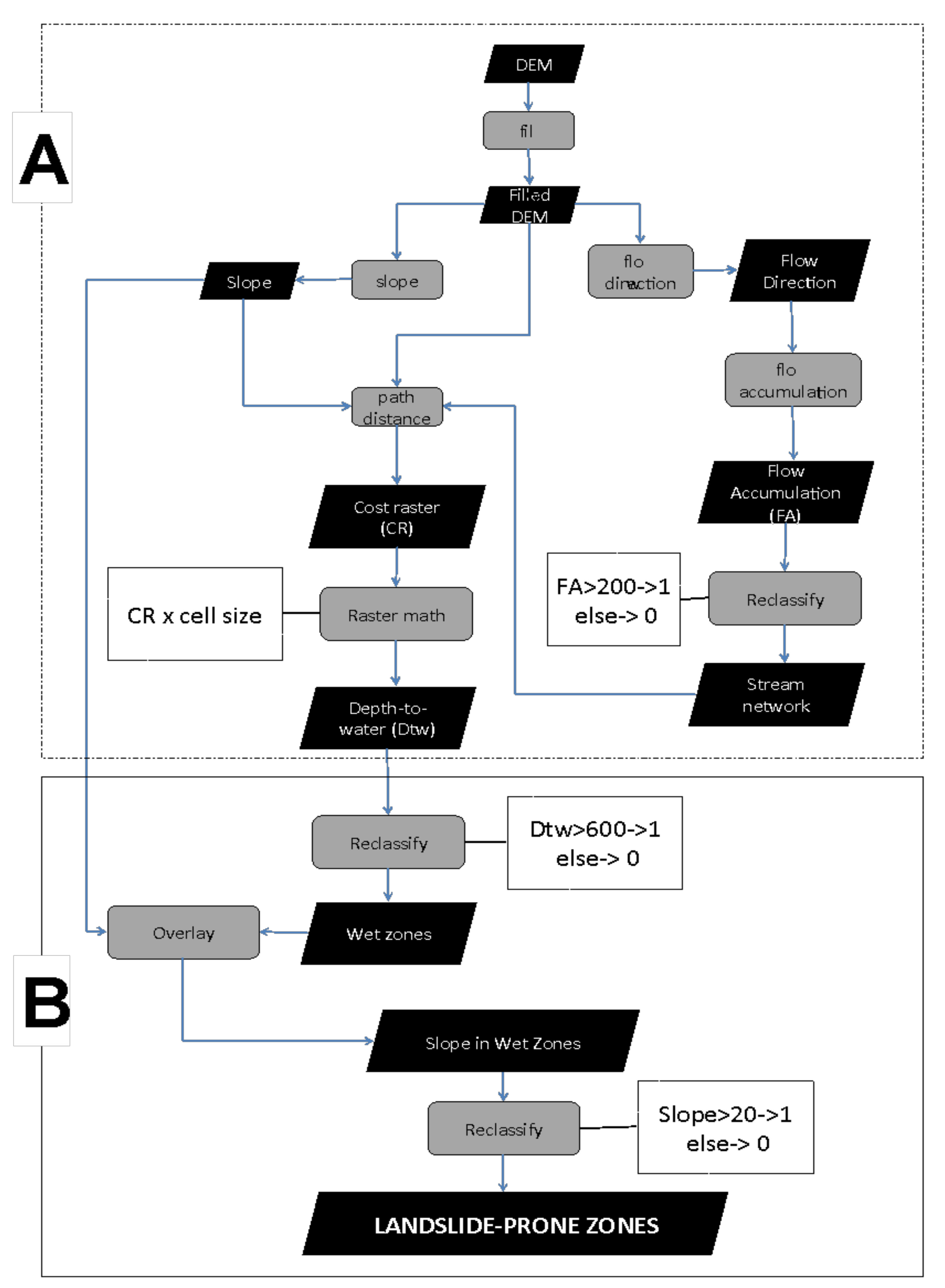
2.2. Detection of Water Accumulation Zones

Water accumulation zones are derived from the calculation of the cartographic depth-to-water index (Dtw; [17]). Dtw is a terrain index that predicts the distance of a given cell in a raster grid to a cell accumulating water. Therefore, the patterns of water flow accumulation (FA) in the landscape must be evaluated first. FA can be assessed with a GIS-based, context operator (e.g., [22]) using a filled or depression-less DEM raster as input. FA operators estimate the likely number of neighbouring raster cells flowing into a given cell (e.g., [23]). Hence, DEM-derived terrain attributes such as the curvature, aspect, and elevation will therefore determine the direction of flow and, eventually, its accumulation. Once FA is estimated, a cost raster (i.e., a raster dataset that identifies the cumulative cost of traveling from every cell in a raster to a specific source; [24]) can be generated by implementing a path-distance algorithm in which the FA, slope gradient, and elevation are used as source, cost, and surface raster, respectively (Figure 1). It is worth noting that the FA dataset needs reclassification into a Boolean raster (i.e., a raster which contains only 0 and 1) to generate a usable source raster. This can be achieved by setting up an appropriate threshold in terms of the number of cells flowing into a particular cell, defining which cells in the FA raster dataset will actually be accumulating water, similarly to how stream networks are defined using GIS-based operation (e.g., [25]; Figure 1A). Eventually and, by definition, Dtw is the product of the cost raster created in the previous step and the raster resolution (Figure 1A; [17]).

2.3. Detection of Landslide-Prone Zones

Zones prone to slope failure will likely, and realistically, present a combination of steep slope gradients and high soil wetness (Figure 1B; [3]). Landscape zones prone to being wet due to the accumulation of water can be derived from Dtw (see Section 2.2; Figure 1A) by establishing arbitrary distance thresholds, or buffers, from and to raster cells into which water will likely flow and accumulate [17]. Distance thresholds may vary with the resolution (i.e., cell size) of the DEM raster employed to generate Dtw. Thus, to establish appropriate distance thresholds and, to ensure that wet zones are adequately delimited for a given study area, it is advisable to identify the pixel or cell value within the Dtw raster at locations where Dtw is high. For example, using a DEM with a resolution of 2 × 2 m2, a threshold value of 600 m was chosen (Figure 1B). Subsequently, a reclassification process can be implemented to generate a Boolean raster in which all those pixels within the established threshold acquire a value of 1 (Figure 1B). The latter step is meant to highlight zones likely to be wet on the landscape and thus likely to present weak soil materials from the geotechnical stand-point [7]. Then, the Boolean raster can be overlaid with the slope raster through a multiplication operation using a raster calculator (i.e., Boolean wet zones raster x slope raster in degrees; Figure 1B). The resulting raster will be comprised of cells containing the slope gradient value for likely wet zones. With the latter, another Boolean raster can be created to select the steepest zones only (e.g., slope gradient > 20; Figure 1B) and, hence, to delimit zones that could be subject to landslide events on the basis of combining steep topography and high soil wetness. The output from the former overlay operation is a Boolean raster in which landslide-prone zones have a value of 1 while the rest of the pixels have a value of zero. The latter can be processed further by replacing the zeros with null values, obtaining discrete polygons denoting zones prone to landslides.

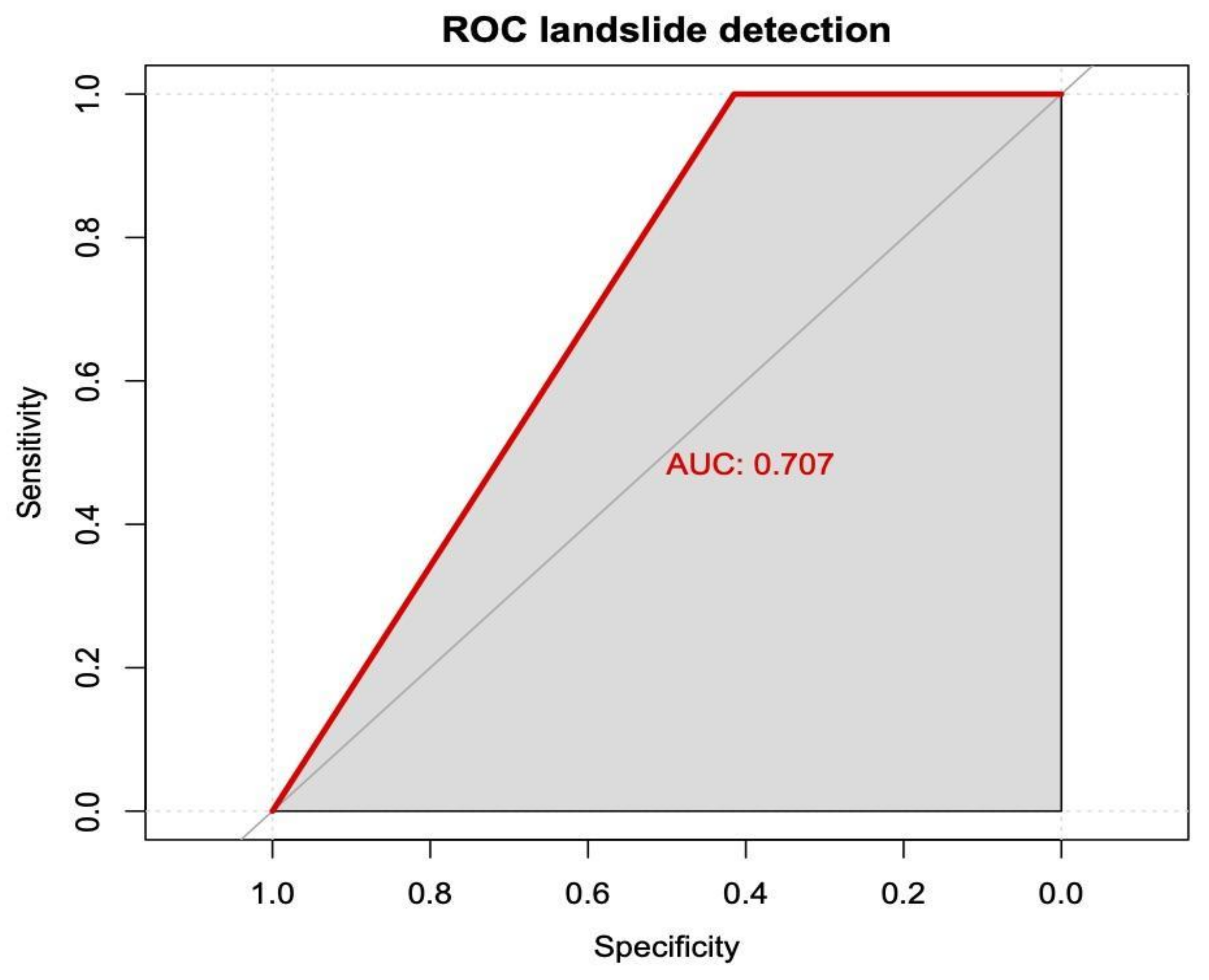
2.4. Tool Verification

To verify the predictive capacity of the proposed tool, the cartographic model shown in Figure 1A,B was implemented on a small-scale, study site with a history of landslide events. To implement the proposed tool, a 2 × 2 m2 resolution DEM was used as input [26] and the steps depicted in Figure 1A,B were implemented in ESRI ArcGIS Desktop v.10.5 [24]. Eventually, the retrieved outcomes were compared against aerial images captured in 2016 and 2017 and provided by ESRI Imagery (http://www.esri.com/arcgis/imagery-remote-sensing/content; accessed on 12 April 2021) and Tomtom-Apple Inc. Maps v2.1, and supplemented with a ground verification process outlined below. The sensitivity, specificity, and accuracy of the proposed tool was assessed through conducting an ROC (receiving operating characteristic curve) analysis (e.g., [27]). To this end, an ROC curve was built by plotting the rate of true positive cases of landslide detection (i.e., sensitivity) against the rate of false positive cases (i.e., 1-specificity). We considered that true positive cases of landslide detection were those landslide-prone zones detected by the proposed tool in which an active or past landslide exists on the ground within the polygon established by the tool. We considered that false positive cases of landslide detection were those landslide-prone zones detected by the tool in which an active or past landslide is not visible on the ground. True negatives were assumed to be those zones in which landslide-prone zones were not detected and where landslides do not actually exist on the ground. The area under the ROC curve (AUR) was calculated using a polygons method with the R package pROC [28].
The study site is adjacent to Catterline Bay, Aberdeenshire, UK (WGS84 Long: −2.21 Lat: 56.90). Catterline Braes (CB) is a 400 m long, 30 m high coastal slope forming the northeastern end of the Catterline Bay, Figure 2). The site is within the maritime climate zone with mild summers and cool winters, relatively narrow annual temperature range with the precipitation being relatively evenly dispersed throughout the year (the mean temperature at the site is 8.9 °C and the mean annual rainfall is 565.13 mm; [29]. Geomorphological studies carried out on the site [19] showed slopes within the site area to be typically inclined at 34° (range: 25–50°) with a general ESE aspect. CB includes a series of exposed slope sections interspersed with gully-outcrop forms ranging in height between 2 and 10 m. A small, 2.0 m wide tarmac-surfaced access road divides the slope into upper and lower, traversing from SW to NE and dropping in level from 26 mAOD (metres above Ordnance Datum) at the SE end to 2.5 mAOD at the pier stage at the NE end of the bay. Twelve private residential properties are located along the crest of the slope that effectively has no owner, with a grassed, non-fenced public footpath offsetting the residential properties from the actual slope. A branch of the footpath leads to a mid-slope structure—a former pumping station used in the past to capture the water from the slope and supply the adjacent residential properties with fresh water. Remnants of a sea defence wall comprising rounded boulders of 200–300 mm diameter exist at the toe of the slope delineating it from the beach. The sea defense wall comprises sections of mass poured concrete gravity wall of trapezoidal cross-section, gabion baskets interconnected with a metal chain of approx. 200 mm diameter links, and an array of concrete cubes of 1 m3 volume. The line of the sea wall is broken and the structures comprising it damaged to various degrees due to the action of the waves and potential seepage from the slope.
There is a history of landslide activity along the slope, demonstrated through the series of hollows, gullies, outcropping rock mounds, and bulges, which represent washouts, near-surface slope failures linked to the springs, and areas of ongoing creep (Figure 3; [31]). Local sources document landslips dating back from the 1950s with the more recent major events (1994, 1995, and 2013 and 2020; Table 1) resulting in creation and enlargement of the gullies and failure scars on the slope. Based on the detailed site inspection, several mechanisms of failure become evident. Translational slips of 0.5–1.0 m depth (Figure 3a) occur mainly on the upper slope in the sparsely vegetated and exposed areas of the slope potentially due to oversteep slopes combined with the surface and/or groundwater acting as a destabilizing agent. These failures are progressive up- or down-slope and result in exposing the superficial soil deposits which are then further eroded by the surface/ground water. At the locations where the surface/ground water is the main driving agent, these slips can take the form of a mudslide or mudflow after a heavy rain or storm event, resulting in deposition of washed-out fine material but also shrubs/small trees and blockage of the access road (Figure 3a). In both cases, the washed-out material blocks the gravel drain, which causes further erosion and instability by running off and penetrating into the soil on the lower slope. Deeper slides (1.0–2.0 m depth) were recorded on the lower slope which may be connected to the stability and retention capacity of the seawall defence. During the event in 2013, high waves topped the seawall and started eroding the lower slope at the same time increasing the pore water pressures in the lower slope. This resulted in instability of the seawall which was destroyed at the gabion sections and dislocated at the concrete block sections. This collapse allowed the movement of the soil on the slope (Figure 3b), which resulted in subsidence of the access road embankment. It is possible that this failure can migrate upslope and lead to further instability, potentially affecting the properties at the crest.
Published geological maps [32] show the superficial soils at the site area (Figure 2) to comprise Raised Beach Deposits (RBD) of sands and gravels of the Quaternary period on the slopes and Mill of Forest Till Formation (Glacial Till) at the crest of the slope. The bedrock is indicated to comprise Catterline Conglomerate Formation of early Devonian age with clasts mainly of lava, but also containing psammite, quartzite, vein-quartz and feldspar porphyry in a medium-grained lithic sandstone matrix. Trial pitting and subsequent laboratory tests [33] carried out at 25 locations across the Upper and Lower slope to depths of 500 mm confirmed the published information and recorded the uppermost soil horizons as 300 mm thick topsoil underlain by reddish-brown gravelly silty sand (sand: 79.82%; silt: 5.85%; clay: 3.08%) of low dry strength and low plasticity [34]. The saturated hydraulic conductivity of this soil (Ks = 5.82 × 10⁻⁵ m s−1) indicates well drained conditions.
A review of satellite imagery from the past 10 years, the land cover maps and field observations from the past four years record the slope to be a neutral grassland covered with a range of vegetation types to a varying degree. Grasses, herbs, shrubs and planted trees are present on the slope, with the coverage varying seasonally from approximately 20% in winter to approximately 80% during the vegetative period. At the crest of the slope and beyond the residential properties, arable and horticultural land use is recorded.
Published hydro-geological maps [35] indicate the superficial aquifers to be of moderate to high productivity with predominantly intergranular flow. The aquifers are indicated to be vulnerable to pollutants not readily adsorbed or transformed [36]. Detailed site inspection showed a visible seepage line at the level of and adjacent to the pumping house, as well as 25 m north of the pumping house, indicating a spring or a series of non-ephemeral springs, which then flows along naturally formed gullies towards a non-maintained gravel drain running along the access road which discharges into the sea at the landing stage. The surface water from the residential properties is discharged mainly near the crest of the slope, and collected in the same gravel drain at the side of the access road.

3. Results and Discussion

The results shown in Figure 4 indicate that the proposed tool is able to satisfactorily detect landslide-prone zones. In addition, 84.7% of the polygons generated by the tool fell on zones presenting slope failure events (i.e., 89 out of 105 polygons), or they appeared to be adjacent to zones with clear landslide signs (i.e., bare zones without vegetation cover; Figure 4 and Figure 5). The slight mismatch between the delimited polygons and landslides featuring in the aerial image (Figure 4) could be due to the differences between the location of landslide initiation and deposition zones [37]. The latter may imply that the proposed tool is mainly capable of detecting landslide initiation zones. In addition, the results suggest that both shallow (i.e., visible in the northern half of the coastal slope; Figure 4) and deeper (i.e., visible in the southern half of the coastal slope; Figure 4) landslides can be detected with the proposed tool. The ROC curve for the proposed landslide detection tool (Figure 5) indicates that the predictive accuracy of the tool is very satisfactory (AUC = 0.707; i.e., there is a 70% chance that the tool will detect a true landslide zone), considering its low input requirements—i.e., just a high-resolution DEM. The ROC curve retrieved from the analysis showed a straight profile because the same set of polygons were used in the ROC analysis following a manual classification into “true” or “false” landslide (Figure 6) rather than using an alternative landslide map for the study area (e.g., [27]). The ROC curve also suggests that the tool presents a satisfactory trade-off between sensitivity and specificity (e.g., [38]). The latter outcome was affected negatively by the size of some landslide-prone polygons classified as “false” positives (Figure 6C). It is worth noting that most of the polygons classified as “false” landslides do not currently show landslide signs because, in reality, they have slope stabilisation elements such as a dense cover of woody vegetation (Figure 7C; [8]) or ground stabilisation structures (i.e., concrete retaining walls; Figure 7D), supporting further the ability of the proposed tool to identify landslide-prone zones in the study area. Therefore, the combination of potentially wet soil and steep zones was effective for detecting zones within the study site, with the added value that both zones can be retrieved from a single DEM raster dataset (Figure 1).
The results of the landslide detection (Figure 4) show a very good correlation with the locations of historic instability at Catterline Braes (Figure 2; Table 1). While the dissipation of pore water pressures and formation of gullies as forms of preferential drainage pathways have locally reduced the risk of instability in the south/east slopes of the Braes (Figure 2), the risk of instability remains relatively high in the north/west part of the Braes, despite the higher frequency of instability on this area of the slope. This can be partially explained by the presence of the non-ephemeral springs in that part of the slope, which have historically been exploited and then capped (Table 1). This action may have blocked the established seepage pathways for the groundwater and expanded them to the north and south of the now disused pumping station where the most recent slip has occurred (Figure 8).
The applicability and veracity of the proposed tool were verified in February 2020 and 2021, respectively, when, after a period of prolonged rainfall, two new landslips occurred (Table 1) in the northern parts of Catterline Braes and below the car park in the access road to the Pier (Figure 4 and Figure 8). These landslips, similar in behaviour to the shallow translational slips recorded on site before (Table 1, Figure 3a) occurring in areas mapped as ‘high risk’ by the proposed tool (framed areas in Figure 4). They originated in areas of high soil wetness where precipitation, potentially combined with groundwater from the non-ephemeral springs, had saturated the soil and created positive pore water pressures, which were then dissipated by a flow over a steeper slope gradient and removal of the uppermost soil horizons along the way to the deposition zone on the beach (Figure 8a) and the access road, which, in turn, was ultimately blocked by the debris (Figure 8b).
The application of the tool proposed herein on a broader scale can provide an insight into the exposure of wider areas (e.g., watershed) to landslides and how these may impact on other hazards such as floods and debris flows (e.g., [39]). However, the spatial resolution of the DEM, which for the present study was of 2 × 2 m2, should be taken into account, as less detailed DEM datasets will likely lead to poorer definitions of landslide-prone zones. In fact, the authors believe that the proposed tool could be of limited use with coarse resolution DEM rasters (i.e., point spacing of kilometers), as the terrain features of the landscape related to surface water accumulation can be hardly portrayed with them at the site scale, so the assumptions behind the proposed tool (Section 2.1) would not hold. This limitation is somehow balanced by the tool’s ability to identify landslide-prone zones using a single input (i.e., DEM; Figure 1). DEM datasets are readily available from spatial libraries (e.g., UK’s Digimap, USGS), making the proposed tool very interesting under data-limited situations. The output from the proposed tool can also be an excellent basis for multi-criteria analysis approaches (e.g., [40]), by which multiple environmental attributes relevant to landslides detection and prediction (e.g., soil type, soil depth, bedrock type, land cover, rainfall intensity, etc.; [3]) can be merged to refine landslide detection and mapping exercises. However, it must be worth noting that our tool can effectively capture two key drivers of slope instability—i.e., surface water accumulation and slope gradient, constituting a simple but robust approach that links both slope topography and hydrology. The proposed tool can thus serve as a basis to gain spatial knowledge about the interaction of different environmental and natural processes, and how those combine to create instability for slopes in a wider area (e.g., watershed) to inform and support workflows for the mitigation and restoration of landslides [20]. A systematic approach like the one suggested by [20], which underpins this tool, will ultimately allow the identification of instability drivers, which, in turn, can allow identification of the most suitable mitigation or protection methods to interrupt the key driving process rather than attempting smaller, potentially more numerous, solutions for providing local remediation.
The spatial nature of the proposed tool’s output makes possible its use in the evaluation and mapping of hazards and risks associated with landslide events (e.g., [40,41,42]), the identification of zones needing slope restoration to avoid instability events [8], the detection of landslides on larger geographical areas or at different spatial scales than the one showcased here, or the generation of real-time land-slide prediction systems if the tool is combined with a more comprehensive evaluation of the soil and climate features.
Once the instability drivers and slope instability hazards have been outlined and mapped using the proposed tool, the management of the potential risks will have to take cognisance of the broader strategy for protection and mitigation before defining and implementing specific investigations. This strategy should be derived in consultation between land owners and the relevant stakeholders. In cases where there is no legal owner of the site at risk, such as the case study site presented here, the relevant stakeholders (residents at and on adjacent sites, recreational users, interest groups and similar) can define the strategy and also provide insight into the history of instability on the site (Table 1), which can form the basis of a more detailed instability inventory [43]; Figure 9).
The detailed investigations should target not only the drivers of instability but also the other elements of the system [20], including the soil, vegetation, flora/fauna, and their interactions. The mitigation measures can be targeting the high-risk areas identified by the GIS-based tool and can be instrumented to provide an insight into their behaviour and effect on the surrounding environment and areas of lower risk. The monitoring data can then be used to provide more detailed information on the interactions between the mitigation measures and the broader environment, which, in turn, will enrich the GIS-based tool with information from which a long-term behaviour can be predicted, perhaps using machine learning algorithms (e.g., [12,29]).
The advantage of the GIS tool presented here is that it can be used and updated by designers and asset managers alike, without much knowledge on GIS, geology, or hydrology, for preliminary landslide hazards mapping. However, we stress that the use of the proposed tool should be supplemented with ground inspection and investigation, and that the actions directed to manage landslide hazards identified by the tool should be designed appropriately by competent experts. Future extensions of the current work may include the investigation of other advanced machine learning and metaheuristic methods to enhance the performance of the landslide detection tool, inclusion of nature-based solution particulars for hazard assessment, inclusion of other factors governing the behaviour of landslides, as well as applying the current tool for hazard management in other study areas.

4. Conclusions

This paper presented a refined, simple, GIS-based tool for the detection of landslide-prone and slope restoration zones. The tool only required a DEM dataset as input to retrieve spatial information on the location of steep and potentially wet soil zones, whose combination allowed detection of both shallow and deeper landslides satisfactorily. The tool is readily implementable at different spatial scales and its output is readily usable in landslide hazards and risk mapping exercises. However, it is advisable to implement the proposed tool in combination with ground investigations collecting information on the geotechnical properties of the slope soil materials, as well as creating a landslide inventory, to ascertain the likelihood of slope failure and hence evaluating the hazards of landslides occurrence more realistically.

Author Contributions

A.G.-O.: Conceptualization; Data curation; Formal analysis; Investigation; Methodology; Software; Validation; Visualization; Writing—original draft; Writing—review & Editing; S.B.M.: Conceptualization; Funding acquisition; Project administration; Supervision; Writing—original draft; Writing—review & editing. All authors have read and agreed to the published version of the manuscript.

Funding

This research was funded by the OPERANDUM project. This project has received funding from the European Union’s Horizon 2020 research and innovation program under grant agreement No. 776848.

Institutional Review Board Statement

Not applicable.

Informed Consent Statement

Not applicable.

Data Availability Statement

The data presented in this study are available on request from the corresponding author. The data are not publicly available due to potential intellectual property rights infringement.

Conflicts of Interest

The authors declare no conflict of interest.

References

  1. European Environmental Agency (EEA). Soil Erosion; Permalink:M2MK6NE2MP; EEA: Brussels, Belgium, 2012. [Google Scholar]
  2. Koutsoyiannis, D. Revisiting the global hydrological cycle: Is it intensifying? Hydrol. Earth Syst. Sci. 2020, 24, 3899–3932. [Google Scholar] [CrossRef]
  3. Lu, N.; Godt, J.; Or, D. Hillslope Hydrology and Stability; Cambridge University Press: New York, NY, USA, 2013. [Google Scholar]
  4. Varnes, D.J. Slope movement types and processes. In Landslides, Analysis and Control, Special Report 176: Transportation Research Board; Schuster, R.L., Krizek, R.J., Eds.; National Academy of Sciences: Washington, DC, USA, 1978; pp. 11–33. [Google Scholar]
  5. Sidle, R.C.; Bogaard, T.A. Dynamic earth system and ecological controls of rainfall-initiated landslides. Earth. Sci. Rev. 2016, 159, 275–291. [Google Scholar] [CrossRef]
  6. Mohan, A.; Singh, A.K.; Kumar, B.; Dwivedi, R. Review on remote sensing methods for landslide detection using machine and deep learning. Trans. Emerg. Telecommun. Technol. 2020, e3998. [Google Scholar] [CrossRef]
  7. Vanapalli, S.K.; Fredlund, D.G.; Pufahl, D.E.; Clifton, A.W. Model for the prediction ofshear strength with respect to soil suction. Can. Geotech. J. 1996, 33, 379–392. [Google Scholar] [CrossRef]
  8. Gonzalez-Ollauri, A.; Mickovski, S.B. Plant-Best: A novel plant selection tool for slope protection. Ecol. Eng. 2017, 106, 154–173. [Google Scholar] [CrossRef] [Green Version]
  9. Gonzalez-Ollauri, A.; Mickovski, S.B. Shallow landslides as drivers for slope ecosystem evolution and biophysical diversity. Landslides 2017, 14, 1699–1714. [Google Scholar] [CrossRef] [Green Version]
  10. Gariano, S.; Brunetti, M.; Iovine, G.; Melillo, M.; Peruccacci, S.; Terranova, O.; Vennari, C.; Guzzetti, F. Calibration and validation of rainfall thresholds for shallow landslide forecasting in Sicily, southern Italy. Geomorphology 2015, 228, 653–665. [Google Scholar] [CrossRef]
  11. Chae, B.-G.; Park, H.-J.; Catani, F.; Simoni, A.; Berti, M. Landslide prediction, monitoring and early warning: A concise review of state-of-the-art. Geosci. J. 2017, 21, 1033–1070. [Google Scholar] [CrossRef]
  12. Zhao, C.; Lu, Z. Remote sensing of landslides—A Review. Remote. Sens. 2018, 10, 279. [Google Scholar] [CrossRef] [Green Version]
  13. Ray, R.L.; Lazzari, M.; Olutimehin, T. Remote Sensing Approaches and Related Techniques to Map and Study Landslides. Landslides Investig. Monit. 2020. [Google Scholar] [CrossRef]
  14. Mondini, A.C.; Guzzetti, F.; Chang, K.-T.; Monserrat, O.; Martha, T.R.; Manconi, A. Landslide failures detection and mapping using Synthetic Aperture Radar: Past, present and future. Earth-Sci. Rev. 2021, 216, 103574. [Google Scholar] [CrossRef]
  15. Vorpahl, P.; Elsenbeer, H.; Maerker, M.; Schröder, B. How can statistical models help to determine driving factors of landslides? Ecol. Model. 2012, 239, 27–39. [Google Scholar] [CrossRef]
  16. Bui, D.T.; Hoang, N.D.; Nguyen, H.; Tran, X.L. Spatial Prediction of Shallow Landslide Using Bat Algorithm Optimized Machine Learning Approach: A Case Study in Lang Son Province, Vietnam. Adv. Eng. Inform. 2019, 42, 100978. [Google Scholar]
  17. White, B.; Ogilvie, J.; Campbell, D.M.H.; Hiltz, D.; Gauthier, B.; Chisholm, H.K.H.; Wen, H.K.; Murphy, N.C.; Arp, P.A. Using the cartographic depth-to-water index to locate small streams and associated wet areas across landscapes. Can. Water Resour. J. 2012, 37, 333–347. [Google Scholar] [CrossRef]
  18. Norris, J.E.; Stokes, A.; Mickovski, S.B.; Cammeraat, E.; van Beek, R.; Nicoll, B.C.; Achim, A. Slope Stability and Erosion Control: Ecotechnological Solutions; Springer: Berlin/Heidelberg, Germany, 2008; 290p. [Google Scholar]
  19. Gonzalez-Ollauri, A.; Mickovski, S.B. Using the root spread information of pioneer plants to quantify their mitigation potential against shallow landslides and erosion in temperate humid climates. Ecol. Eng. 2016, 95, 302–315. [Google Scholar] [CrossRef] [Green Version]
  20. Lee, E.M.; Brunsden, D. Sediment budget analysis for coastal management, west Dorset. Geol. Soc. Lond. Eng. Geol. Spéc. Publ. 2001, 18, 181–187. [Google Scholar] [CrossRef]
  21. Jones, D.K.C.; Lee, E.M. Landsliding in Great Britain; HMSO: London, UK, 1994; 361p. [Google Scholar]
  22. Eastman, J.R.; Fulk, M.; Toledano, J.; Hutchinson, C.F. The GIS Handbook; USAID: Washington, DC, USA, 1993. [Google Scholar]
  23. Zhu, X. GIS for Environmental Applications: A Practical Approach; Routledge: New York, NY, USA, 2016. [Google Scholar]
  24. ESRI. ArcGIS Desktop: Release 10.5. Redlands; Environmental Systems Research Institute: Redlands, CA, USA, 2016. [Google Scholar]
  25. Vieux, B.E. Distributed Hydrologic Modeling Using GIS; Springer Nature: Berlin/Heidelberg, Germany, 2016. [Google Scholar]
  26. GetMapping. GetMapping 2m Resolution Digital Surface Model (DSM) for Scotland and Wales; NERC Earth Observation Data Centre: Leicester, UK, 2014; Available online: http://cataloque.ceda.uk/uuid/4b0ed418e30819e4448dc89a27dc8388 (accessed on 21 April 2021).
  27. Chung, C.-J.F.; Fabbri, A.G. Validation of spatial prediction models for landslide hazard mapping. Nat. Hazards 2003, 30, 451–472. [Google Scholar] [CrossRef]
  28. Robin, X.A.; Turck, N.; Hainard, A.; Tiberti, N.; Lisacek, F.; Sanchez, J.-C.; Muller, M.J. pROC: An open-source package for R and S+ to analyze and compare ROC curves. BMC Bioinform. 2011, 12, 77. [Google Scholar] [CrossRef]
  29. Gonzalez-Ollauri, A.; Thomson, C.S.; Mickovski, S.B. Waste to Land (W2L): A novel tool to show and predict the spatial effect of applying biosolids on the environment. Agric. Syst. 2020, 185, 102934. [Google Scholar] [CrossRef]
  30. Apple Maps; Apple, Inc: Cupertino, CA, USA.
  31. Mickovski, S.B.; Santos, O.; Ingunza, P.M.D.; Bressani, L. Coastal slope instability in contrasting geo-environmental conditions. In Geotechnical Engineering for Infrastructure and Development—Proc. XVI European Conference for Soil Mechanics and Geotechnical Engineering, Edinburgh, Scotland, September 2015; Institute of Civil Engineers: London, UK; pp. 1801–1806.
  32. BGS (British Geological Survey). 1:50000 Geology [SHAPE Geospatial Data], Scale 1:50000, Tiles: sc067, Updated: 1 October 2013; BGS (British Geological Survey): London, UK, 2013. [Google Scholar]
  33. BS 1377. Methods of Test for Soils for Civil. Engineering Purposes, Parts 1–9; British Standards Institution: London, UK, 1990.
  34. BS EN 14688. Geotechnical Investigation and Testing—Identification and Classification of Soil, Parts 1–2; British Standards Institution: London, UK, 2004.
  35. Macdonald, A.M.; Ball, D.F.; Dochartaigh, B.É.Ó. A GIS of Aquifer Productivity in Scotland: Explanatory Notes; CR/04/047N; British Geological Survey Commissioned Report; BGI: London, UK, 2004; 21p. [Google Scholar]
  36. SNIFFER. Development of a Groundwater Vulnerability Screening Methodology for the Water Framework Directive; Final Report, Project WFD28; SNIFFER: Edinburgh, UK, 2004. [Google Scholar]
  37. Walker, L.R.; Velázquez, E.; Shiels, A.B. Applying lessons from ecological succession to the restoration of landslides. Plant. Soil 2009, 324, 157–168. [Google Scholar] [CrossRef]
  38. Zou, K.H.; O’Malley, A.J.; Mauri, L. Receiver-Operating Characteristic Analysis for Evaluating Diagnostic Tests and Predictive Models. Circulation 2007, 115, 654–657. [Google Scholar] [CrossRef] [Green Version]
  39. Jackson, B.M.; Wheater, H.S.; McIntyre, N.R.; Chell, J.; Francis, O.J.; Frogbrook, Z.; Marshall, M.; Reynolds, B.; Solloway, I. The impact of upland land management on flooding: Insights from a multiscale experimental and modelling programme. J. Flood Risk Manag. 2008, 1, 71–80. [Google Scholar] [CrossRef]
  40. Gonzalez-Ollauri, A.; Mickovski, S.B. Hydrological effect of vegetation against rainfall-induced shallow landslides. J. Hydrol. 2017, 549, 374–387. [Google Scholar] [CrossRef] [Green Version]
  41. Gonzalez-Ollauri, A.; Stokes, A.; Mickovski, S.B. A novel framework to study the effect of tree architectural traits on stemflow yield and its consequences for soil-water dynamics. J. Hydrol. 2020, 582, 124448. [Google Scholar] [CrossRef]
  42. Van Westen, C.J.; van Asch, T.W.J.; Soeters, R. Landslide hazard and risk zonation—Why is it so difficult? Bull. Eng. Geol. Environ. 2006, 65, 167–184. [Google Scholar] [CrossRef]
  43. Soeters, R.; Van Westen, C.J. Slope Instability Recognition, Analysis and Zonation. In Landslides, Investigation and Mitigation, Transportation Research Board, National Research Council, Special Report 247; Turner, A.K., Schuster, R.L., Eds.; National Academy Press: Washington, DC, USA, 1996; pp. 129–177. [Google Scholar]
Figure 1. Cartographic model for the GIS-based tool for detecting landslide-prone zones. (A) steps for calculating the carto-graphic depth-to-water index (Dtw); (B) steps for detecting landslide-prone zones by overlaying steep and potentially wet soil zones. Black boxes: raster layer; Grey boxes: GIS-based operations; White boxes: reclassify operations specific details for this case study.
Land 10 00685 g001
Figure 2. Study area. Circles denote approximate locations of historic (pre-2021) failures. Source image: [30].
Land 10 00685 g002
Figure 3. (a) typical translational slips; (b) typical deeper-seated slips on the study site.
Land 10 00685 g003
Figure 4. Landslide-prone zones detected by the proposed tool in Catterline Bay. Framed areas indicate the location of a landslip after the hazard mapping was completed (see Figure 8). Capital letters in white are related to the close-ups shown in Figure 7.
Land 10 00685 g004
Figure 5. ROC curve and area under the curve (AUC) for the proposed landslide detection tool.
Land 10 00685 g005
Figure 6. Over 84% of the polygons detected as landslides by the proposed tool (A) fell in zones presenting real signs of landslides within the study site; (B) The remaining 16% of the polygons did not belong to zones with active landslides; (C) Most of study site’s surface is not subjected to landslides, being the proposed tool effective in classifying these areas as “true” negative landslide polygons (D). The labeled polygons (A), (B), (C), and (D) are shown in Figure 7.
Land 10 00685 g006
Figure 7. Polygons (A) and (B) were detected by the proposed tool on zones with signs of landslides whilst polygons (C) and (D) were detected as “false” positives (see Figure 6). A landslip event occurred in the area delimited in polygon (A) in February 2020 (see Figure 8). Source Images: [30].
Land 10 00685 g007
Figure 8. Landslips that occurred in (a) February 2021 and (b) 2020 in areas previously mapped as ‘high risk’ by the proposed GIS-based tool (Figure 4).
Land 10 00685 g008
Figure 9. The application of the new proposed GIS-based tool for landslip detection within the process for management of slope instability.
Land 10 00685 g009
Table 1. Historic records of failures on the slopes of the case study site.
YearEventConsequence
1958Major slip above the south pier of the harbourCollapse of a road section
1950s–1970sDrains and water supply channels blockedVegetation overgrowth
1980sSlope failure at far western endMajor damage to residential property
1992Distortion of the carriageway surfaceCracked pavement
1993-Localised bulging of the slope and development of longitudinal cracking along the footpath on the embankment
1994Slope failures above and below the road due to heavy continuous rainfall over a period of 4 daysRoad blockage
2009Surface washouts and mud flows at the south-east end; major slip at the far western endUndermined road embankment; major damage and abandonment of residential property
2013Storm surge, erosion of the slope toeBreached seawall defence
2020Slope failure initiated mid-slope after a period of continuous rainfall (occurred after the completion and verification of the model)Road blockage
2021Slope failure initiated below the road on the southern extent of the access roadUndermined and exposed existing road drainage infrastructure
Publisher’s Note: MDPI stays neutral with regard to jurisdictional claims in published maps and institutional affiliations.

