Article

A Two-Stage Approach to the Estimation of High-Resolution Soil Organic Carbon Storage with Good Extension Capability

1
Guangxi Key Laboratory of Forest Ecology and Conservation, College of Forestry, Guangxi University, Nanning 530004, China
2
Faculty of Forestry, University of British Columbia, Vancouver, BC V6T 1Z4, Canada
3
Guangdong Academy of Forestry, Guangzhou 510520, China
*
Author to whom correspondence should be addressed.
Land 2021, 10(5), 517; https://doi.org/10.3390/land10050517
Submission received: 26 March 2021 / Revised: 7 May 2021 / Accepted: 11 May 2021 / Published: 13 May 2021

Abstract

:
Soil organic carbon storage (SOCS) estimation is a crucial branch of the atmospheric–vegetation–soil carbon cycle study under the background of global climate change. SOCS research has increased worldwide. The objective of this study is to develop a two-stage approach with good extension capability to estimate SOCS. In the first stage, an artificial neural network (ANN) model is adopted to estimate SOCS based on 255 soil samples with five soil layers (20 cm increments to 100 cm) in Luoding, Guangdong Province, China. This method is compared with three common methods: The soil type method (STM), ordinary kriging (OK), and radial basis function (RBF) interpolation. In the second stage, a linear model is introduced to capture the regional differences and further improve the estimation accuracy of the Luoding-based ANN model when extending it to Xinxing, Guangdong Province. This is done after assessing the generalizability of the above four methods with 120 soil samples from Xinxing. The results for the first stage show that the ANN model has much better estimation accuracy than STM, OK, and RBF, with the average root mean square error (RMSE) of the five soil layers decreasing by 0.62–0.90 kg·m−2, R2 increasing from 0.54 to 0.65, and the mean absolute error decreasing from 0.32 to 0.42. Moreover, the spatial distribution maps produced by the ANN model are more accurate than those of other methods for describing the overall and local SOCS in detail. The results of the second stage indicate that STM, OK, and RBF have poor generalizability (R2 < 0.1), and the R2 value obtained with ANN method is also 43–56% lower for the five soil layers compared with the estimation accuracy achieved in Luoding. However, the R2 of the linear models built with the 20% soil samples from Xinxing are 0.23–0.29 higher for the five soil layers. Thus, the ANN model is an effective method for accurately estimating SOCS on a regional scale with a small number of field samples. The linear model could easily extend the ANN model to outside areas where the ANN model was originally developed with a better level of accuracy.

1. Introduction

Against the background of global warming, the accurate estimation of soil organic carbon storage (SOCS) has become a massive task faced by the forestry and ecological circles. Due to the different data acquisition platforms available in China, putting forward an accurate and useful SOCS estimation standard and method [1] is urgently needed for SOCS-related research to progress. In recent years, the amount of research on soil organic carbon (SOC) and SOCS has increased, both domestically and overseas [1,2], with a mean annual growth rate of 9%. Emerging SOCS estimation methods have been promoted by a few researchers. The existing SOCS estimation methods can be roughly classified into three categories: Soil-type methods, life-zone methods, and modelling methods. A recent study showed that 93 of the 500 previously published papers on carbon storage focus on soil carbon estimation, among which 79 (84.9%) used the soil-type method [2]. The soil-type method has a high frequency of use in soil carbon estimation research due to its simple calculation method and concise results. However, due to its shortcomings, such as the use of different data sources and calculation inconsistency, the soil-type method’s estimation accuracy is low [3]. Except for the estimation result, extra information cannot be obtained through this method. Recently researchers have rarely adopted the life-zone method [4], which estimates the SOCS based on the Holdridge Life Zone Classification System, because the broad life-zone classification does not take the region’s characteristics and heterogeneity into consideration. Regarding the modelling method, there are two main categories. Firstly, there are statistical models, including regression models and spatial interpolation model [5,6]. Since statistical models have strict requirements in terms of data characteristics [7,8], it is hard to meet the requirements for their use in some cases. The other type of model is machine learning, including random forest (RF), support vector machine (SVM), and artificial neural network (ANN) methods. These can use temperature, soil physicochemical properties, precipitation, and other factors as parameters for model training [9]. Machine learning is a burgeoning type of algorithm for SOCS estimation. A study [10] concerning how RF, SVM, and ANN perform when taking precipitation, topographic, and remote sensing variables as model inputs with the highest resolution of 30 m showed that the ANN has a moderate capability to carry out SOCS estimation and digital mapping.
In order to estimate SOCS, different researchers have developed criteria for soil profile division. Huang indicated that, in China, SOCS aggregates on the surface [11]. The majority of studies have concentrated on the surface layer [12,13] or a 1 m deep soil profile [14,15], which has led to few pieces of research focusing on the SOCS below the surface at divided depths [16]. A previous study [17] showed that SOCS accounts for 46–63% of the entire soil profile at depths of 30–100 cm. Therefore, the research subject should be changed to the SOCS below the surface layer to reveal its distribution characteristics. In previous studies on divided depth calculation and the analysis of SOCS, global or regional scales have been used [18], resulting in low-resolution predicted maps, which may have led to homogenization of the results on a regional scale. Others have tended to unevenly stratify the soil profile [19,20], for instance, the soil profile depth below 50 cm was merged into one layer. Such methods cannot display the actual vertical distribution pattern of SOCS.
The objective of this study was to develop a two-stage approach to estimate SOCS with a good extension capability, as follows: (1) The artificial neural network (ANN) model was adopted to estimate SOCS based on 255 soil samples with five soil layers (20 cm increments to 100 cm) in Luoding, Guangdong Province. This was compared with three commonly used methods: The soil-type method (STM), ordinary kriging (OK), and Radial basis function (RBF) interpolation. (2) A linear model was introduced to capture the regional differences and further improve the estimation accuracy of the Luoding-based ANN model when extending it for use in Xinxing, Guangdong Province after assessing the generalizability of the above four methods with 120 soil samples from Xinxing.

2. Materials and Methods
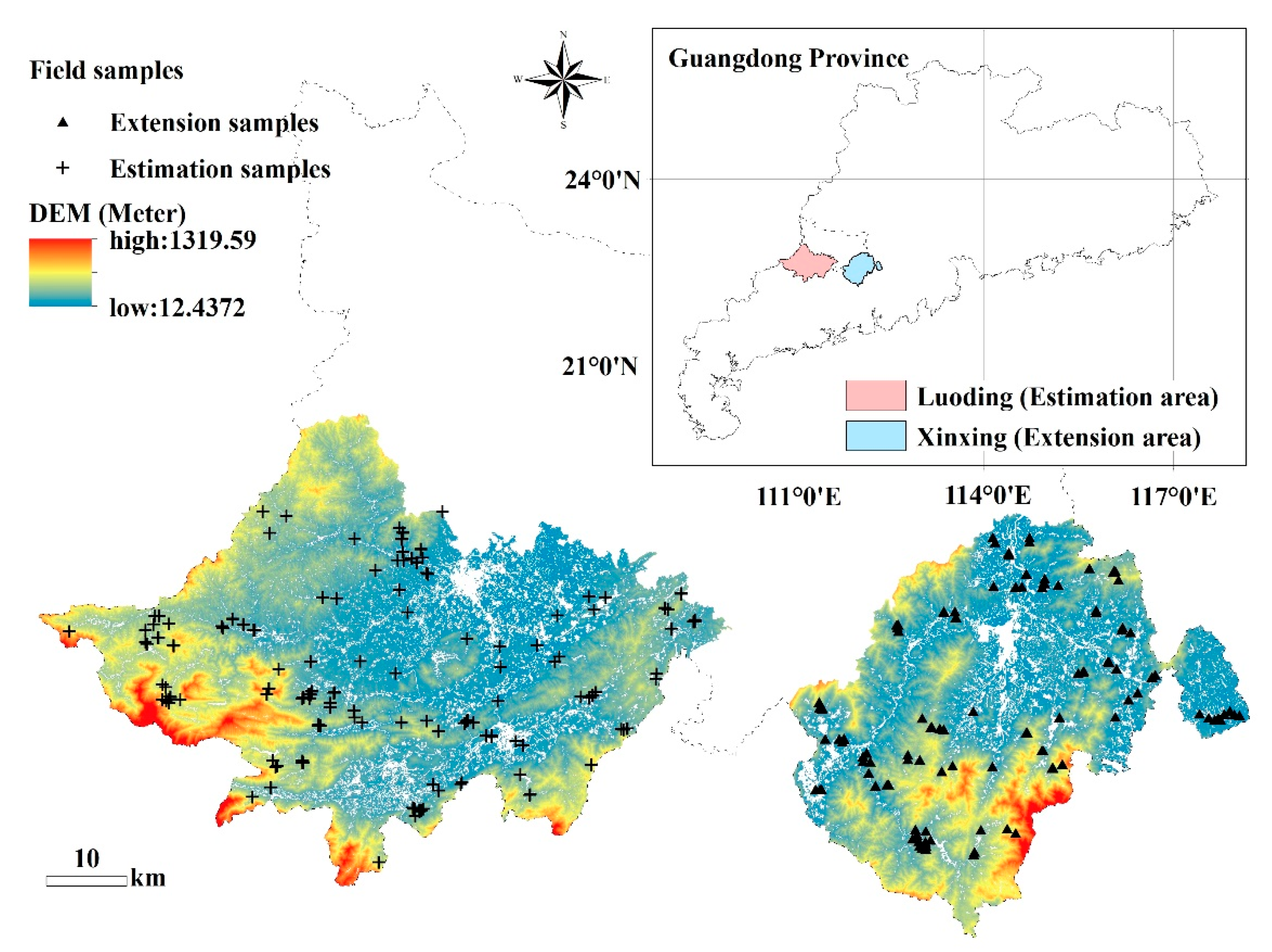
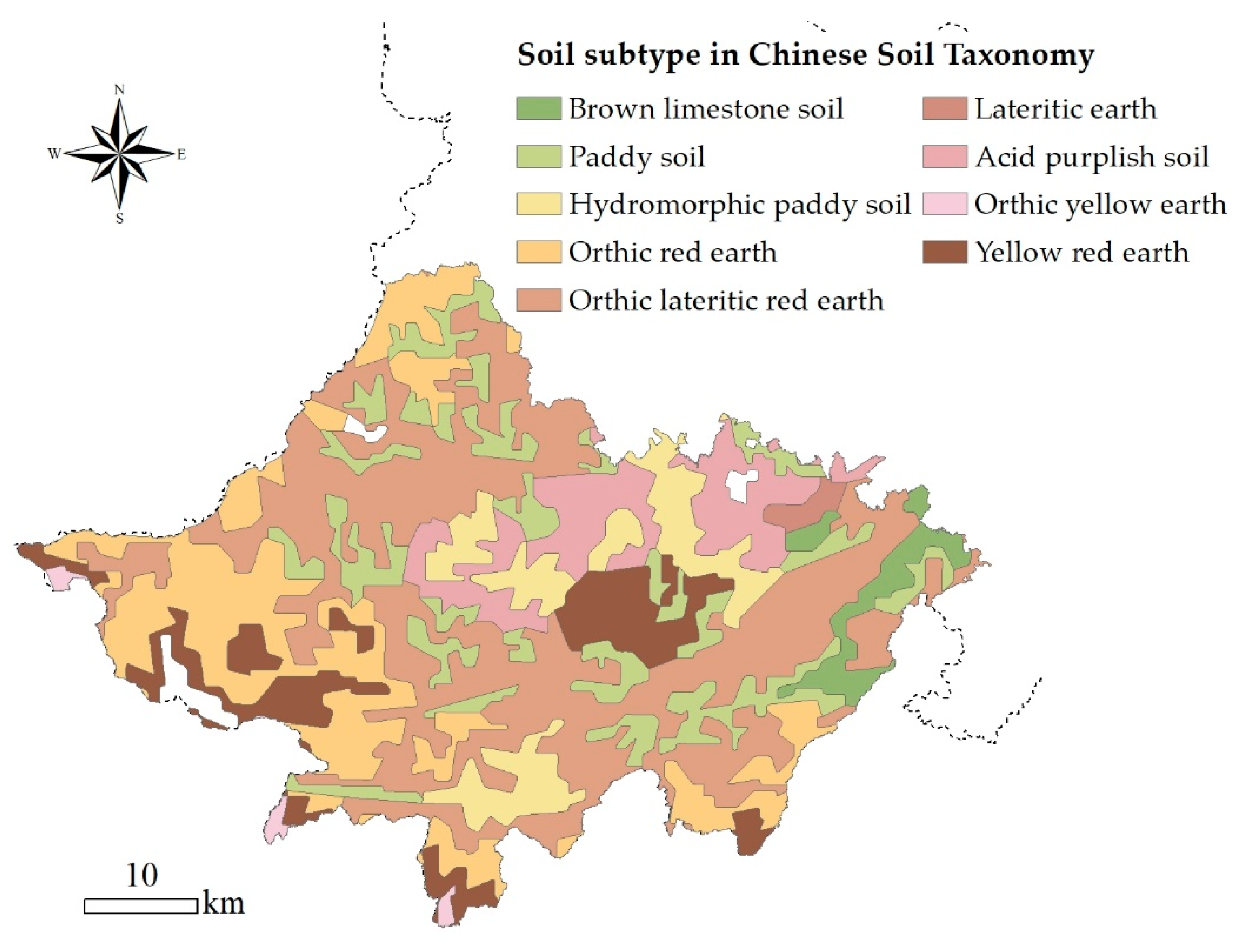
2.1. Study Area

The study area included the entire forest area of Luoding and Xinxing (22°22′–22°58′ N, 111°03′–112°32′ E) in Yunfu City, Guangdong Province, China (Figure 1). The two study areas were in the subtropical monsoon zone with high temperatures and rich precipitation in the same months (from May to October) [21]. The total study area was 3860.5 km2, with Luoding and Xinxing accounting for 2327.5 and 1533 km2, respectively. The primary geomorphic type in the study area was hills [22], and the elevation ranged from 12.4 to 1319.6 m with a mean of 224.6 m. There were different forest types present, including natural secondary evergreen broad-leaved forest, coniferous forest, and mixed forest. The main tree species present were Cunninghamia lanceolata (Lamb.) Hook., Eucalyptus robusta Smith, and Pinus massoniana Lamb. [23]. The soil parent materials included granite, sand shale, and erosive parent materials [21]. The soil zone of the study area was the lateritic red earth zone of the south Asian subtropical monsoon rain forest. The mean soil thickness in the Luoding and Xinxing study areas was 107.8 and 99.3 cm, respectively.

2.2. Field Sample

Soil profile data for Luoding (Estimation area) and Xinxing (Extension area) were obtained from Guangdong Academy of Forestry Sciences as part of an investigation and evaluation in a forest soil nutrient survey project that began in 2015 [23]. In total, 345 soil profiles were collected, of which 225 and 120 samples came from Luoding and Xinxing, respectively. Each profile was divided into five layers: 0–20 cm (L1), 20–40 cm (L2), 40–60 cm (L3), 60–80 cm (L4), and 80–100 cm (L5). The excavation depth of the profiles was either 1 m or to the parent material layer if a profile’s thickness was less than 1 m. A total of 1695 samples were collected from 345 soil profiles with 3–5 layers. The bulk density (BD) was measured by the ring (core) method [24,25]. The BD was calculated with Equation (1), and its statistics are listed in Table 1. The soil samples were air-dried in the laboratory stage and then sieved through 3, 2, and 0.25 mm sieves. The weight and volume of the gravel (diameter > 2 mm) were recorded. The soil organic matter (SOM) content of soil samples was measured by the potassium dichromate-titration method [26]. Then, the SOM values of the soil samples were transformed into the SOCD using Equation (2):
B D s = ( M × 100 ) V × ( 100 + w )
S O C D s = B D s × S O M s × T × 0.58 × ( 100 α ) 100 × 10 2
where B D s is the bulk density of the samples (g·cm−3), M is the original weight of the soil (g), w is the soil water content (as a percentage), V is the cylinder’s volume (cm3). S O C D s is the soil organic carbon density (kg·m−2) of the samples, T is the thickness of the soil layer (cm), S O M s is the SOM content of the samples (g·kg1), 0.58 is the Bemmelen coefficient [27], and α is the percentage of rock fragments (gravel) in the soil with diameters greater than 2 mm.

2.3. Other Data and Materials

The coarse resolution 0–20 cm soil organic matter map (CSOM) was obtained from the Atlas of Guangdong soil on a scale of 1:2,800,000 and was compiled by the Guangdong soil survey team (Guangdong Soil Survey Team, 1993). Then, it was transferred to a digital map within a geographic information system. The content of coarse-resolution soil organic matter (CSOM) in the map was delineated at six levels (Level 1: greater than 40 g/kg; Level 2: 30–40 g/kg; Level 3: 20–30 g/kg; Level 4: 10–20 g/kg; Level 5: 6–10 g/kg; Level 6: <6 g/kg; National soil survey office, 1998). This study applied the CSOM as the required input parameter for the ANN model to represent the general conditions of SOM in a region. For the purposes of modelling and map production, the CSOM map was converted from features to a raster map with a 10 m resolution after the levels of the maps were numbered.
The digital elevation model (DEM) data obtained from Guangdong Academy of Forestry Sciences were derived from stereo images of Cartosat-1 (IRS-P5) with a 12.5 m resolution [28] and resampled to a 10 m resolution to meet the map production needs. The spatial analyst extension and developed Forest Hydrology Tools of ArcGIS [29,30] (ArcGIS 10.2 for Desktop. Version 10.2.0.3348. RedLands, Esri Inc., Redlands, CA, USA) were used to derive four topographic variables, slope, aspect, topographic position index (TPI), and potential solar radiation (PSR), and five hydrological variables, the soil terrain factor (STF), sediment delivery ratio (SDR), depth to water (DTW), flow length (FL), and flow direction (FD). The TPI refers to the relative topographic position of the central point, which is the difference between the elevation of this point and the mean elevation of a predetermined neighborhood [31,32]. The SDR is the ratio of the sediment transported to the outlet to the total erosion in the watershed area [33]. The DTW refers to the elevation differences between the land and the nearest water surfaces [34,35]. This study applied nine variables derived from the DEM model as the candidate parameters for the ANN model input.
A soil-type map (Figure 2) with a 1:1,000,000 scale was downloaded from the Soil SubCenter, National Earth System Science Data Center, National Science and Technology Infrastructure of China (http://soil.geodata.cn (accessed on 1 June 2020)) [36]. The classification units used in this study were subtypes. Lateritic earth was present in the greatest frequency in both Luoding and Xinxing, accounting for 37.1% and 69.4% of the total area, respectively. Additionally, for the purpose of map production, the soil-type map was converted from features to a raster map with a 10 m resolution after the classes of the maps were numbered.

2.4. The First Stage: SOCS Estimation Methods

2.4.1. The Artificial Neural Network (ANN) Estimation Method

1. ANN modeling. This study applied the back-propagation ANN (BP-ANN) because it can accommodate nonlinearity when limited discontinuous points are available between the input and output data [37]. This ANN model was trained with a back-propagation technique, which adjusted the weight and bias values along a negative gradient descent to minimize the mean squared error (MSE) between the network outputs (predicted values) and the targeted values (measured values) [38]. The BP-ANN model had a three-layer structure: an input layer, an output layer, and a hidden layer. The input layer was made up of several predictors (required parameters and candidate parameters) with 2–10 nodes according to the parameters’ combination. The output layer contained one node, SOCD. The number of hidden layer nodes was 35, and this was determined based on previous studies [39,40]. An early stopping method was used to quickly confirm the fittest model coefficients and avoid over-fitting [41]. The early stopping method divided the training data into a training subset and test subset, in which the latter was used to test the training error by the end of a training period. In this process, if the training root mean square error (RMSE) decreased while the testing RMSE increased, the early stopping method stopped the training [42]. The programming was implemented in Matlab software (Matlab (R2016a). Version 9.0.0.341260. Natick, The MathWorks Inc., Natick, MA, USA).
2. Selection of model inputs. This study took the CSOM maps as the required parameter and the nine topographic and hydrological variables derived from the 10 m resolution DEM data as the candidate parameters. These parameters were used because the CSOM was able to capture the SOCS at regional scales, providing basic data support for the ANN model. The DEM-derived variables were able to modify the SOCS on the local scale [39]. Each combination of candidate parameters corresponded to an ANN model. For the nine parameters the number of combinations, as calculated by C 9 1 + … + C 9 9 , was 511 [39,40].
The required parameter, the candidate parameters, and 90% of soil samples in Luoding were input into the ANN model. We chose the optimal combination of candidate parameters with the best accuracy through 10-fold cross-validation. In the 10-fold cross-validation mode, the modeling dataset (90% of soil samples) was divided into 10 equal subsets. A model was built with data in nine subsets as the calibration data, and this was validated with the remaining subset as validation data; this process was repeated 10 times until all subsets were used in the validation set [39].
3. SOCD estimation. After obtaining the optimal SOCD prediction values and the spatial distribution maps with 10 m resolution for five soil layers, we were able to calculate the SOCS of each layer by multiplying the forest area of Luoding with the mean SOCD of each layer.

2.4.2. The Common Estimation Methods

1. The soil type method (STM): This study used ArcGIS 10.2 software (ArcGIS 10.2 for Desktop. Version 10.2.0.3348. RedLands, Esri Inc., Redlands, CA, USA) to extract soil subtype information from 90% of soil samples from a soil type map at a scale of 1:1,000,000 (Figure 2). After obtaining the information on the corresponding subtypes from 90% of the soil samples, the SOCD of each subtype at the Ln layer was calculated using Equation (3) (for subtypes not covered by samples, the SOCD was replaced by the mean SOCD of all subtypes in the mapping process). Then, the SOCD and SOCS of a soil layer were determined using Equations (4) and (5), respectively:
S O C D t n = s = 1 x S O C D s t × ( 100 α ) 100 x
S O C D n = t = 1 9 S O C D t n 9
S O C S n = S O C D n × A × 10 3  
where S O C D t n is the soil organic carbon density (kg·m−2) of a subtype (refers to “t” in the equation) at the Ln soil layer, S O C D s t is the soil organic carbon density (kg·m2) of samples belonging to subtype t, x is the number of samples within subtype t, and α is the percentage of rock fragments (gravel) in the soil with diameters greater than 2 mm. S O C D n is the soil organic carbon density of the Ln soil layer. S O C S n is the soil organic carbon storage (Tg) of the Ln soil layer and A is the area of Luoding (km2).
2. Ordinary Kriging (OK): The samples used for OK interpolation had to meet the intrinsic hypothesis or second stationary assumption. Additionally, the samples had to obey a normal distribution. This study adopted the number field sieve method to identify the extremum by using samples’ mean values to add or subtract three-fold standard deviations [43]. The extremum, which is outside the number field, was replaced by extreme values within the number field. For the first step, a semivariogram (Equation (6)) using the field samples was expressed as a function of the distance between sampled points, and the integrity of spatial continuity was calculated in one or multiple directions. We chose the optimal model from the Gaussian, exponential, and spherical models to form the experimental semivariograms [44,45,46]. The semivariogram analysis of OK was conducted using GS+9.0 software. The second step of OK interpolation was to calculate the values of unknown points as weighted sums of the adjacent samples’ SOCD values (Equation (7)) [47,48]:
γ ( h ) = 1 2 N ( h ) h = 1 N ( h ) [ Z ( x i ) Z ( x i + h ) ] 2
Z x = i = 1 n γ i Z ( x i )
where γ ( h ) is the semivariogram for the distance interval class h known as lag, N ( h ) is the number of paired samples in the lag interval, and Z ( x i ) and   Z ( x i + h ) are the sample’s SOCD values at two points separated by the distance interval h . Z ( x ) is the value to be estimated at location x , and n is the number of sites within the search neighborhood used for the SOCD estimation.
3. Basis Function (RBF): The RBF is suitable for calculating a large number of samples. It can achieve smooth interpolation by calculating a set of weighted coefficients of the nodes through the basis function. The RBF method involves the use of a family of five deterministic exact interpolation techniques: The inverse multi-quadric function, the multi-quadric function, the spline with tension, the completely regularized spline, and the thin-plate spline [6,44]. Of these five functions, the spline with tension with the lowest error was selected for SOCD interpolation.
The interpolation process of OK and RBF was achieved using the Geostatistical Analyst module in ArcGIS 10.2 software (ArcGIS 10.2 for Desktop. Version 10.2.0.3348. RedLands, Esri Inc., Redlands, CA, USA).

2.5. Extension Test of the Four Estimation Methods

This part of the study was conducted to determine the extension capability of the four methods when facing a nearby area with similar hydrological and geological conditions to the estimation area (Luoding). The four estimation methods only extended their results estimated in Luoding to Xinxing, and no soil profile data from Xinxing were adopted. The accuracy assessment of the extension results used 80% of the soil profile data from Xinxing.

2.6. The Second Stage: The Linear Model for Extending the ANN Estimation Method

The aim of building the linear model was to modify the SOCD estimated by the ANN method to adapt the geological differences over a large extended area, so we used Xinxing as the test area. Besides improving the ANN model’s estimation accuracy at Xinxing, the linear model used a small number of field samples to reduce the sampling cost. In line with Zhao’s research [39], 1/5 soil samples can be used to build a steady linear model; hence 20% of soil samples from Xinxing were randomly selected as the modelling data for the linear model in this study. The other 80% of the samples were applied for validation. In the first step, we used Matlab software (Matlab (R2016a). Version 9.0.0.341260. Natick, The MathWorks Inc., Natick, MA, USA) to produce maps of Xinxing by adopting the Luoding-based ANN model. In this process, we did not use any data from Xinxing. In the second step, linear model building used SOM levels from the CSOM map for classification, which meant that one level corresponded to a linear model. In the CSOM map, the proportions of SOM from Xinxing from high to low were 45.2%, 44.0%, 10.6%, and 0.2% of the total area for Level 3, Level 5, Level 4, and Level 2, respectively. In the calculation process, we merged Level 2 with Level 3 and classified the 120 soil profiles of Xinxing according to their corresponding levels. Subsequently, 20% of the soil samples from each level were selected to build a corresponding linear model (Equation (8)):
S O C D e = a i + b i · S O C D A N N
where S O C D e is the adapted SOCD. S O C D A N N is the initial SOCD estimated by the Luoding-based ANN model. i is an SOM Level of Xinxing. a i is the shifting parameter, which describes the average difference in SOCD between the ANN model area (Luoding) and the extended linear model area (Xinxing). b i is the stretching parameter, which describes the rate of change in SOCD between Luoding and Xinxing.

2.7. Accuracy Assessment

The estimation results for Luoding were validated by 10% of the Luoding soil samples, and the extended accuracy validation used 80% of the soil samples from Xinxing. Three indices were adopted to describe the accuracy: the root mean square error (RMSE), the determination coefficient (R2), and the mean absolute error (MAE). The calculations used were as follows:
R M S E = i = 1 n ( X m , i X p r e , i ) 2 N
R 2 = 1 i = 1 n ( X p r e , i X p r e , i ^ ) 2 i = 1 n ( X p r e , i X p r e , i ¯ ) 2
M A E = i = 1 n | X m , i X p r e , i | N
where X m , i is the measured value, X p r e , i is the predicted value, N is the number of samples, X p r e , i ^ is the fit value, and X p r e , i ¯ is the mean of predicted value.

3. Results

3.1. Statistical Characteristics of the Field SOCD

As Table 2 shows, the mean SOCD of the soil profiles decreased from L1 to L5, and the mean SOCD of L1 was double that of L5 in both study areas. The sharpest decrease in the mean SOCD, a decline of approximately 1 kg·m−2, occurred from L3 to L4. Additionally, the mean SOCD of Xinxing at each layer greater than that in Luoding. The CV shows that all soil layers had a moderate level of variation in both study areas under the CV classification standard [46]. The skewness near 0 and kurtosis near 3 showed that the data followed a normal distribution. As Table 2 shows, the data had a skewed distribution at each layer.

3.2. The First Stage: SOCS Estimation Methods

3.2.1. Accuracy of SOCS Estimation Methods

The accuracy levels of the four methods verified by the estimation samples were generally higher than the validation accuracy levels, as shown in Table 3. For the ANN method, the R2 verified by the estimation samples at all soil layers exceeded 0.8, which was the best modelling accuracy. The accuracy of OK verified by the estimation samples was better than that of the RBF for each soil layer. The STM, which generally had R2 values lower than 0.3, showed a poor estimation capability.
The accuracy levels of the four methods are shown in Table 3. For the RMSE and MAE indices, the STM, OK, and RBF had higher values than the ANN method. The low R2 of the STM indicates that the estimation results have little reference significance. For the two interpolation methods, the R2, which was between 0.13 and 0.37 at L1–L3, declined dramatically at L4 and L5. The R2 of the ANN was generally higher than that for the three other methods, especially at L1, L4, and L5. For the STM, its R2 was lower than for the ANN by 0.77, 0.57, 0.50, 0.70, and 0.74 at L1–L5, respectively, with a mean of 0.66. For the OK, its R2 was lower than for the ANN by 0.69, 0.33, 0.27, 0.77, and 0.76 at L1–L5, respectively, with a mean of 0.56. For the RBF, its R2 was lower than for the ANN by 0.65, 0.36, 0.22, 0.68, and 0.78 at L1–L5, respectively, with a mean of 0.54.

3.2.2. Results of SOCS Estimation Method

Figure 3 represents the SOCD distribution estimated by the four methods at L1–L5. The results display a decreasing trend for SOCD with an increase of soil depth. The SOCD estimation results for the whole soil profile are higher with the RBF than with the other methods and are 9.5% higher than the ANN estimation method. The results with the OK are 3.1% higher than with the ANN estimation method. Thus, we can reasonably speculate that the SOCS values estimated by the RBF and OK may lead to higher values. The results estimated by the STM are quite similar to those obtained with the ANN method, only 1.0% lower than the results for the ANN across the whole soil profile. Although the STM is not an effective method for the estimation of samples, the results are still reliable when the mean value is considered.
In terms of the SOCS estimation results (Figure 4), all methods show that the SOCS values at L1 and L2 account for approximately half of the 0–100 cm soil profile. The mean SOCS proportions in L3, L4 and L5 are 21%, 16% and 14%, respectively, and the total proportion is 51%. Therefore, the other half of the SOCS exists in L3–L5. This result is consistent with Batjes’s [17] conclusion that the SOCS in the soil profile of 30–100 cm accounts for 46–63% of the whole profile. This result demonstrates that the SOCS is divided in half at a depth of about 40 cm in relation to the whole profile (0–100 cm).

3.2.3. The Correlation between ANN Model Parameters and the Predicted SOCD

As Table 4 (blot fonts) shows, the combination of candidate parameters adopted by the ANN model is not in accordance with the Pearson correlation, because machine learning methods like ANN are black box methods [7] that cannot reveal the functional relationships between the target and predictor variables [10]. Therefore, we performed the Pearson correlation to analyze the functional relationships between the parameters and SOCD predicted with the ANN model.
The CSOM was significantly correlated with the predicted SOCD at a soil profile of 0–100 cm. For the candidate parameters, the slope had a significant positive correlation with SOCD at L1–L4, which agreed with previous research [47,48] showing that the slope is a strong determinant of the SOCD distribution. Researchers have mostly discussed how the slope affects the SOC distribution in horizontal space, and there are still opposing viewpoints for different factors [21,49]. Our study focused on the correlation between the slope and SOCD with a vertical distribution. According to Table 4, the positive correlation proves that the larger the slope is, the weaker the human influence appears, which provides a favorable environment for SOC aggregation. The slope has no correlation with the SOCD under the 80 cm soil layer, which indicates that the SOCD under the 80 cm soil layer is not affected by the slope. The STF was found to be negatively correlated with the SOCD at L1–L4. The STF is used to define the hydrologic similarity between points [50], which only describes the influence of terrain on streamflow formation [51]. This study deduced that a higher STF represents higher streamflow activity, and higher streamflow activity prevents the SOC accumulation process occurring. It is worth pointing out that the nine hydrological and topographic parameters of L5 did not correlate with SOCD. We deduced that the hydrological and topographic parameters had little influence on the SOCD under the 80 cm soil profile where the SOCD was low and the SOM had been deposited on the bottom for a long period of time.

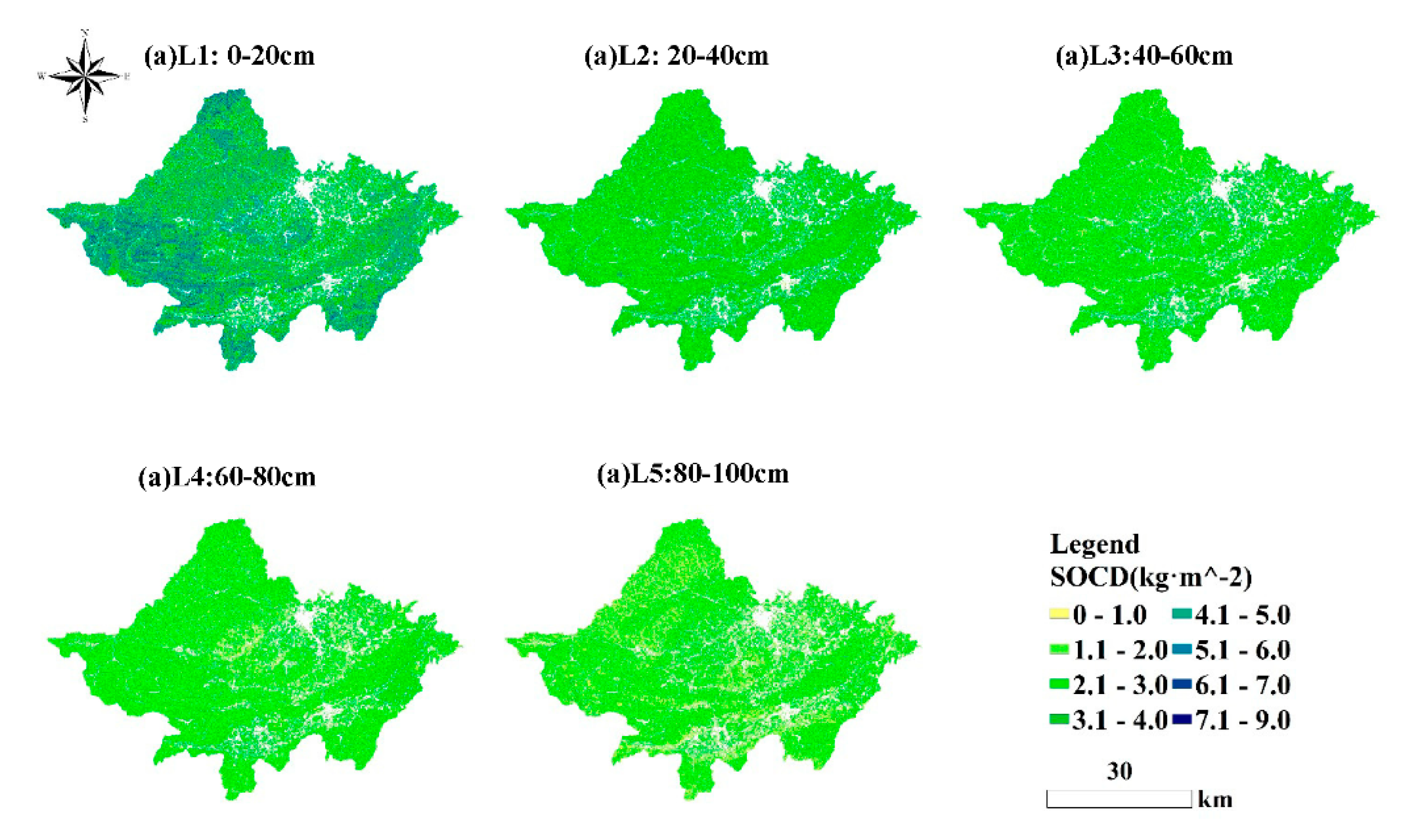
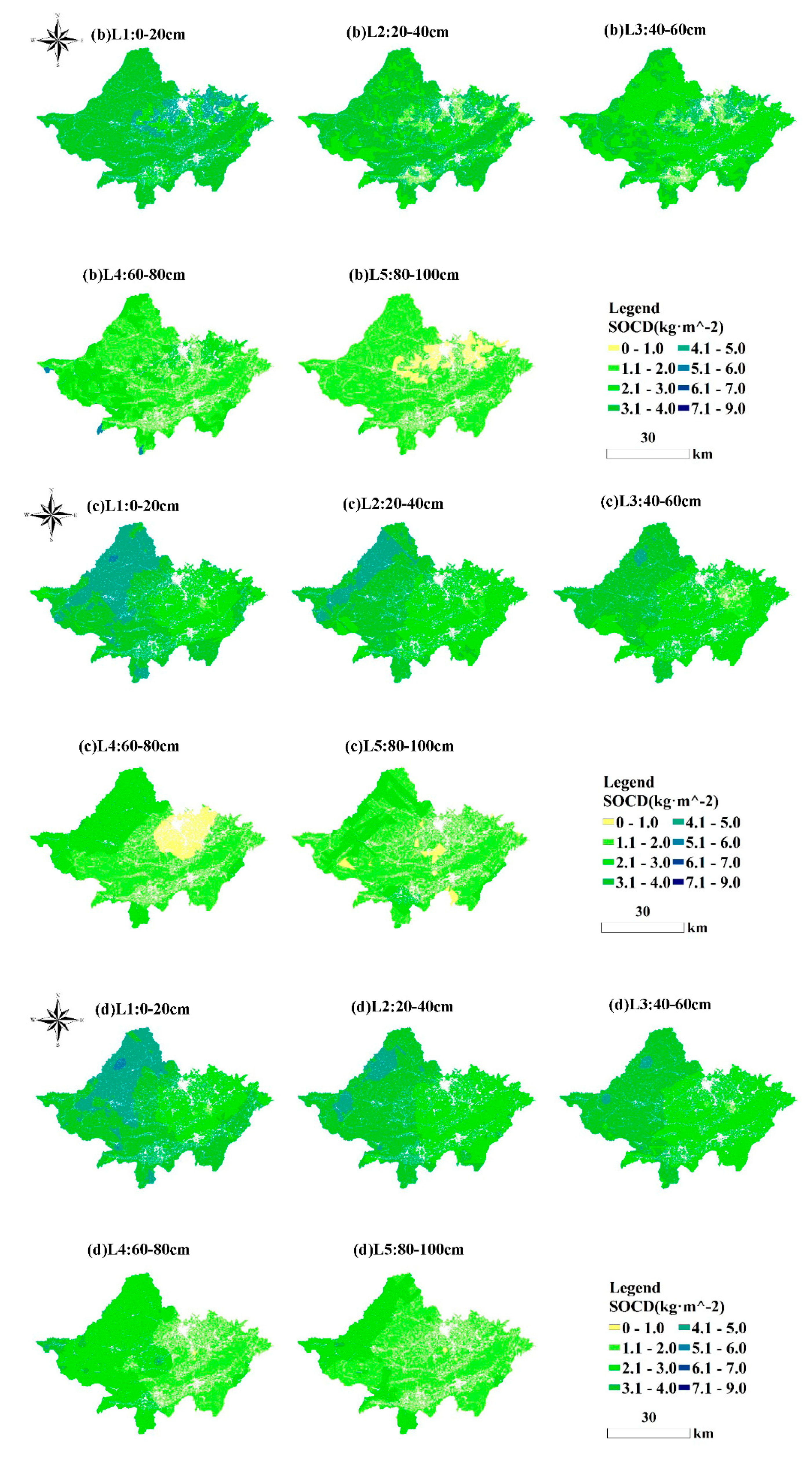
3.2.4. Spatial Mapping of SOCD Estimation Methods

For the ANN estimation method, the SOCD at L1 was found to be comparatively high among the five layers, as shown in Figure 5a, with an evident fluctuation trend, which shows that the SOCD of the southwest grid exceeded 5.0 kg·m−2. Under L1, similar to the estimation results, the SOCD in L1–L4 decreased evenly. However, the maps of L2–L4 were slightly indistinct across the overall SOCD spatial distribution. At L2 and L3, an apparent difference in the spatial distribution maps appeared in the western hilly areas with elevations above 150 m, where the SOCD was generally greater than 3.1 kg·m−2. The main difference between the ANN and the other three methods was that the ANN maps can portray a change of detail in grid resolution. However, except for L1, regional differences were not distinctly displayed on the maps, which is a weakness of ANN model mapping.
For the soil type method, the classification of patches is completely based on the soil-type map, so the SOCD distribution cannot be clearly described. Moreover, mapping is also restricted by the number of samples, which means that when fewer samples are owned by the subtype, the estimation result is less reliable. Taking the map of L4 as an example (Figure 5b), the map shows that the SOCD is higher in the northeast than in the surrounding areas, which is contrary to the results of the other three methods. In practice, areas with abnormal values all belong to one soil subtype, which has merely one corresponding soil sample within 90% of soil samples. The abnormal values resulted in a notable rise in the CV, 63.2% at this layer, while the CVs of the other layers were lower than 30%. This reveals the defect of STM in spatial mapping.
For the OK and RBF, the bull’s eye effect of the RBF (Figure 5d) resulted in an unsmooth surface, especially at L4. However, the OK maps were smooth and not affected by extreme values of samples. This shows that the RBF has a strict demand for sample values, which significantly affects the map’s smoothness. In terms of the variation tendency from L1 to L5, the SOCD values continuously declined. The SOCD in the west region of Luoding was lower than in the northeast region. However, the overall SOCD at L5 predicted by the two interpolation methods was less than 3 kg·m−2, showing a relatively flat variation in SOCD. The 10 m resolution maps produced by the ANN estimation method have the capability to precisely portray the detail of the SOCD distribution. The RBF and OK can only describe the SOCD in grid resolution. Additionally, the RBF map displayed a bull’s eye effect, leading to an unsmooth surface. Similarly to the two interpolation methods, the STM only describes the difference in SOCD in grid resolution, where a soil subtype corresponds to one result. Therefore, it is difficult to determine the precise distribution of SOCD through the STM map.

3.3. Extension Results of SOCD Estimation Methods

Table 5 shows the accuracy of the extension results. The R2 index of STM, OK, and RBF did not exceed 0.1, which suggests that the three methods have little generalizability when there is no data from the target area to support the methods’ operation. The accuracy of estimation results obtained by extending the Luoding-based ANN model to Xinxing was relatively high. However, compared with the validation accuracy in Luoding (Table 2), the R2 decreased by 43–56%, the RMSE rose by 0.60–0.82 kg·m−2, and the MAE rose by 35–78%. The level of error increased significantly, and the mean R2 was lower than 0.5.
Compared with the high accuracy and low error rate of the ANN method in Luoding, the accuracy level in Xinxing was unacceptable. Because of the low estimation accuracy under similar topographic and hydrologic circumstances between Luoding and Xinxing, we suggest that the accuracy of the ANN estimation method may decrease greatly when the two target areas have a larger distance and different circumstances. Therefore, the ANN model performs poorly when extended to a new area. Nevertheless, of all the estimation methods, only the ANN method has the ability to improve. To further improve the accuracy, the linear model was added to tackle this weakness of the ANN estimation method to improve the generalizability.

3.4. The Second Stage: The Linear Model

3.4.1. Coefficients and Accuracy of the Linear Model

The linear model of each layer was built based on the CSOM Levels of Xinxing presented in Table 6. By using 20% of soil samples from Xinxing to build the linear model, the accuracy improved significantly compared with the results shown in Table 5. From L1 to L5, the mean RMSE declined by 0.65, 0.33, 0.32, 0.59, and 0.39 kg·m−2, respectively. The mean MAE declined by 33%, 17%, 20%, 34%, and 28%, respectively. The mean R2 increased by 0.29, 0.23, 0.25, 0.27, and 0.27, respectively. As shown in Table 6, only two sample points from level 4 were used for model building, which led to lower R2 values for the three CSOM levels at each layer. Nevertheless, despite using a small number of samples to build a linear model, which may have resulted in lower accuracy, we conclude that the linear model still effectively improved the ANN estimation method′s estimation accuracy for an extended area.

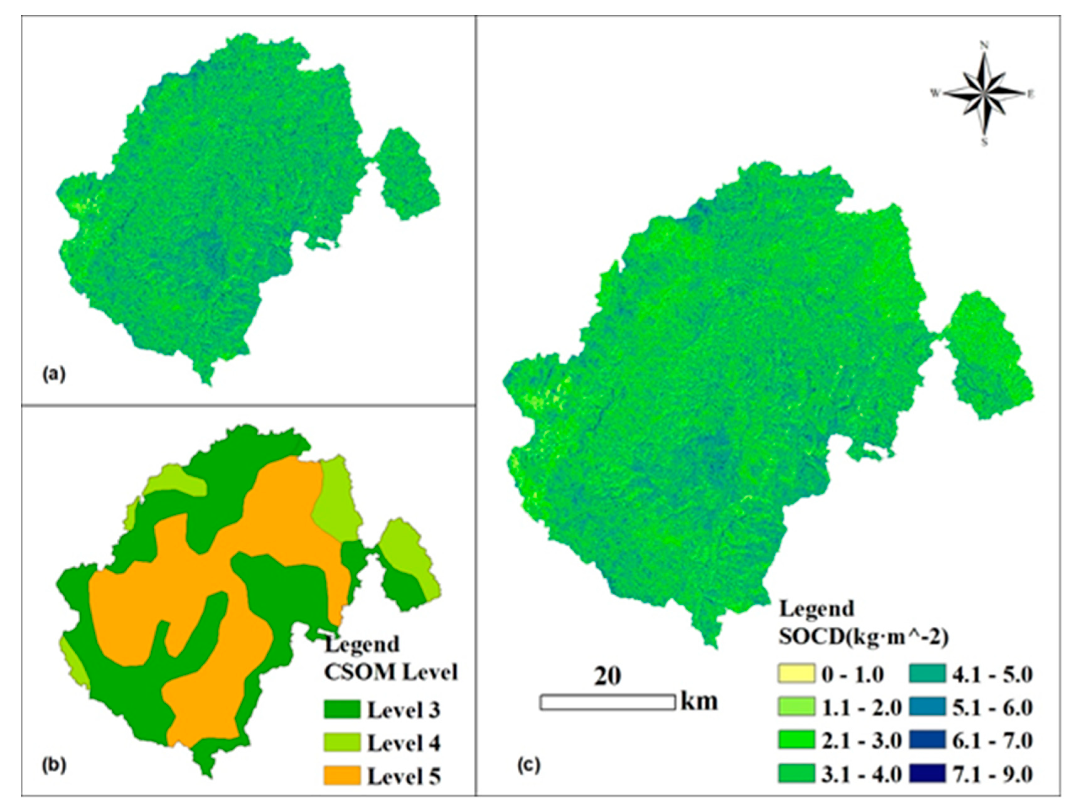
3.4.2. Spatial Distribution Maps of the Extended Area

The Xinxing SOCD spatial distribution map at L1 modified by the linear model for which the R2 index was the highest, shown in Figure 6c, improved the R2 by 0.29. The original SOCD map of Xinxing extended by the Luoding-based ANN model is shown in Figure 6a, and it did not involve the input of any data from Xinxing. To allow a distinct contrast, the water bodies were not removed from the maps.
According to Table 5, the accuracy of Level 4 was lower than at the other two levels, and it is shown in Figure 6c that the SOCD of Level 4 patches was distinctly lower than that of other levels. On the one hand, the linear model based on CSOM level was able to effectively modify the original extended data to give a higher level of accuracy, which allowed is to produce 10 m resolution maps and results using only the linear model and 24 soil samples. We should emphasize that the linear model operates under the condition of having one already-built ANN model. On the other hand, the small number of input samples and the use of coarse-resolution SOM maps could lead to deviations on the map. As shown in Figure 6c, the original boundary of the CSOM map was still visible. We should point out that the variation in the patches at level 4 was not accurate because the boundaries between the levels in the CSOM map were portrayed artificially, and they do not exist in reality.

4. Discussion

4.1. Estimation Capability of the Four Methods

1. The ANN model method. The estimation accuracy of the ANN decreased at L2 and L3 because of the low CV of samples. We speculate that when applying profile data with low CV values, the ANN method’s estimation accuracy is relatively inferior. However, the accuracy of the ANN method was higher than that of the other three methods, and the mean R2 of the five soil layers was 0.78. Meanwhile, the ANN method produced SOCD spatial distribution maps that could reveal the local-scale variation with a resolution of 10 m. One drawback was that the overall variation of SOCD at L2–L4 on the regional scale was somewhat vague, which means we could not obtain more distribution information from these maps. This drawback may become our next focus in improving the mapping capability and evaluating the impact of parameters on mapping.
2. The Soil type method. In the accuracy assessment, The STM had the worst level of accuracy in every soil layer. It performed the worst because the STM is a taxonomic statistical method, which means that its estimation results are based on soil taxonomy but estimated value of sample. As the estimation result showed, the 0–100 cm SOCD result of the STM was the nearest to the ANN method, revealing that the STM’s estimation results could be credible when the mean value is considered. The STM’s accuracy would be significantly affected by the profile data and number of samples, making the STM an imprecise SOCS estimation method at the point dimension.
3. The two interpolation methods. The accuracy of the two interpolation methods showed a similar pattern: the accuracy declined sharply at L4 and L5. The following factors may cause this decline: (i) The spatial distribution of file samples was uneven and aggregated and (ii) some samples at L4 and L5 layers may reach the parent material layer, leading to a high CV value. Especially for deterministic interpolation methods like the RBF, a significant fluctuation of data within a short distance greatly affects the interpolation accuracy, which illustrates the relatively strict data requirements of the interpolation method [7]. We suggest that the interpolation method is not suitable for estimating the SOCS of bottom layer soil. As the estimation results showed, the SOCD values at 0–100 cm estimated by OK and RBF, especially the values of the RBF, were higher than those obtained with the ANN method. We conclude that the ability of the two interpolation methods to perform SOCD estimation of the profile data of this study is lower.

4.2. Extension Capability of ANN Model Estimation Method

In this paper, the linear model is chosen as the extension model to meet the requirements of a small number of samples and simple operability. Theoretically, a stable linear model could be established with a number of samples twice that of its independent variables. Therefore, only 20% of the soil samples were selected to establish the linear model in this study. As the results showed, the ANN model extension results modified by the linear model met the expectations of this study. However, because SOCS changes are affected by human activities, natural conditions [52,53], and many other factors, simply describing the statistical relationship between samples and predicted values with a linear model might cause a poor fitting result. The prediction results are also directly affected by the sample quality. Once the sample outliers appear, the linear model′s prediction result will deviate from the actual situation. This study found that the linear models built at level 4 had lower modeling accuracy because of the small number of samples, but the relationship between number of samples and accuracy was not further discussed. Thus, the next task related to the use of the linear model in extension is to find the relationship between number of samples and model accuracy and to determine the upper limit value of the accuracy.
For the linear model building classification criteria, the CSOM causes a distinct boundary in the distribution maps. This result demonstrates that taking the CSOM map as the model building criteria was effective but may affect our judgment on the real SOCS distribution law. To avoid this condition, finer or other classification maps could be introduced as the linear model building criteria and the potential of the linear model in the ANN model generalization could be further explored.

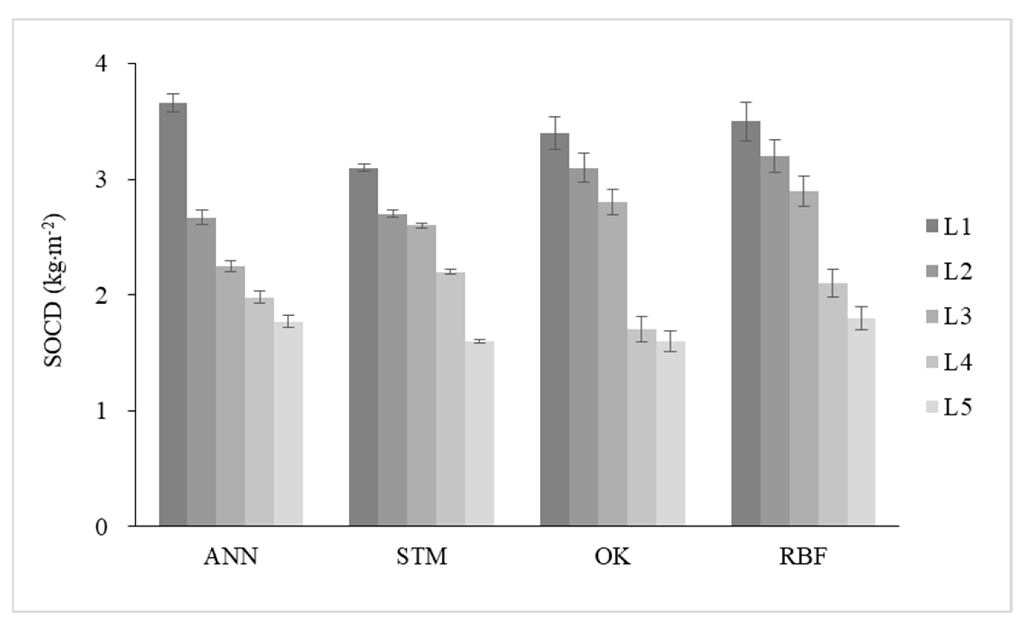
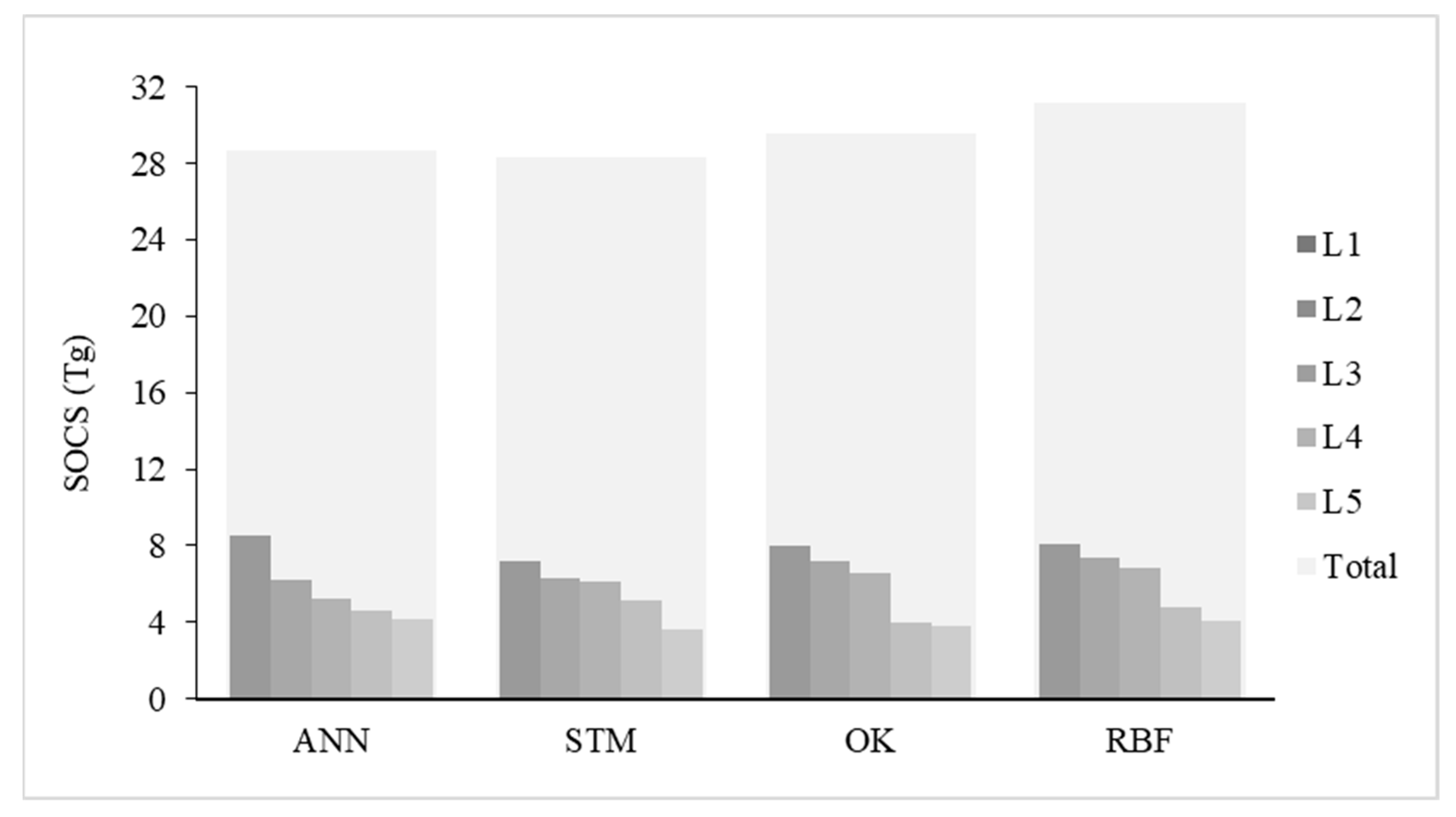
4.3. SOCS Vertical Distribution of the Estimation Area

The results show that the SOCS of all soil layers in Luoding decreased with the soil depth, and the SOCS of L1 accounted for 30% of the 0–100 cm soil layer. We verified that Luoding’s SOCS significantly gathers at the soil surface (0–20 cm) by comparing our results with those of other research. For example, Xie et al. [54] concluded that the SOCS at a soil layer of 0–20 cm accounted for 32.5% of the 0–100 cm soil layer in China; Li et al. [55] found that the SOCS at 0–20 cm accounted for 38.7% of the total in Eastern China; and Chen et al. [56] estimated the SOCS results in Fujian Province and concluded that the SOCS at 0–20 cm accounted for 39.3% of the 0–100 cm soil layer. We suggest that the proportion of Luoding’s surface SOCS is relatively low. In terms of the SOCS in the 0–100 cm soil layer, on a global scale, according to previous studies [4,17,57,58], the global average SOCD of the 0–100 cm soil layer is about 10.6 kg·m−2. Using the scale of terrestrial ecosystems in China, Liang et al. [59] predicted that the average SOCD in the 0–100 cm soil layer in China is about 10.31 ± 3.39 kg·m−2, and Xu et al. [9] predicted that the terrestrial SOCD in China is about 9.13 ± 0.87 kg·m−2. Compared with the SOCD of the 0–100 cm soil layer (12.1 kg·m−2) predicted by the ANN model in Luoding, it is evident that Luoding has a higher level than the national level. The comparison results indicate that the SOCD is relatively high in Luoding, but it does not concentrate in the surface layer (0–20 cm).

5. Conclusions

Our results demonstrate that the ANN estimation method had the best performance in terms of the estimation accuracy and spatial distribution mapping when used to assess data obtained from Luoding City, Guangdong Province, China. The generalization test demonstrated that the soil-type method, Ordinary Kriging, and Radial basis function have little generalizability. The extension results for the linear model built with only 24 samples show that it is practical to improve the estimation results of the ANN model. Thus, the ANN estimation method is an effective method for obtaining accurate SOCS estimation results on a regional scale. By adopting a linear model approach, the ANN estimation method can effectively extend the estimation region with only a small number of field samples with a preferable level of accuracy. However, one drawback of this study is the classification of the linear model. In future research, we will try to use a higher resolution and more precise mapping as the classification criteria to build the linear model to remove the artificial boundary.

Author Contributions

Conceptualization, Z.Z. and S.W.; methodology, S.W. and Z.Z.; software, Z.Z. and S.W.; validation, S.W.; formal analysis, Q.Y. and Z.Z.; investigation, Z.Z. and X.D.; resources, X.D.; data curation, X.D.; writing—original draft preparation, S.W.; writing—review and editing, S.W. and Z.Z.; visualization, Q.Y.; supervision, Z.Z.; project administration, X.D.; funding acquisition, Q.Y. All authors have read and agreed to the published version of the manuscript.

Funding

This work was supported by funding from the Guangxi Natural Science Foundation of China (Grant No. 2018GXNSFAA050135 and 2018GXNSFBA138035), and Guangdong Forestry Science and Technology Plan of China (Grant No. 2019-07). The authors are also grateful to the special founding from Guangxi Hundred-Talent Program to Zhengyong Zhao and Qi Yang.

Institutional Review Board Statement

Not applicable.

Informed Consent Statement

Not applicable.

Data Availability Statement

Not applicable.

Conflicts of Interest

The authors declare no conflict of interest.

References

  1. Zhou, M.; Xiao, H.; Nie, X. Analysis and Prospect of Soil Organic Carbon Research Process in Recent 30 Years at Home and Abroad. Res. Soil Water Conserv. 2020, 27, 395–404. (In Chinese) [Google Scholar]
  2. Sun, W.; Liu, X. Review on carbon storage estimation of forest ecosystem and applications in China. For. Ecosyst. 2020, 7, 37–50. [Google Scholar] [CrossRef] [Green Version]
  3. Song, Y.; Wang, K. Research progress of Forestry Ecosystem Soil Carbon Storage Accounting Methods at Home and Aboard. J. Green Sci. Technol. 2018, 1–6. (In Chinese) [Google Scholar] [CrossRef]
  4. Post, W.M.; Emanuel, W.R.; Zinke, P.J.; Stangenberger, A.G. Soil carbon pools and world life zones. Nature 1982, 298, 156–159. [Google Scholar] [CrossRef]
  5. Hengl, T.; Heuvelink, G.B.M.; Rossiter, D.G. About regression-kriging: From equations to case studies. Comput. Geosci. 2007, 33, 1301–1315. [Google Scholar] [CrossRef]
  6. Bhunia, G.S.; Shit, P.K.; Maiti, R. Spatial variability of soil organic carbon under different land use using radial basis function (RBF). Model. Earth Syst. Environ. 2016, 2, 17. [Google Scholar] [CrossRef]
  7. Lei, X. Applications of machine learning algorithms in forest growth and yield prediction. J. Beijing For. Univ. 2019, 41, 23–36. (In Chinese) [Google Scholar]
  8. Li, Q.; Yue, T.; Fan, Z.; Du, Z.; Chen, C.; Lu, Y. Spatial simulation of topsoil TN at the national scale in China. Geogr. Res. 2010, 29, 1981–1992. (In Chinese) [Google Scholar]
  9. Xu, L.; Yu, G.; He, N.; Wang, Q.; Gao, Y.; Wen, D.; Li, S.; Niu, S.; Ge, J. Carbon storage in China’s terrestrial ecosystems: A synthesis. Sci. Rep. 2018, 8, 2806. [Google Scholar] [CrossRef] [PubMed]
  10. Kennedy, W.; Dieu, T.B.; Dick, Ø.B.; Singh, B.R. A comparative assessment of support vector regression, artificial neural networks, and random forests for predicting and mapping soil organic carbon stocks across an Afromontane landscape. Ecol. Indic. 2015, 52, 394–403. [Google Scholar]
  11. Huang, Y.; Guo, Z.; Wu, Z.; Chai, M. Accuracy Analysis of Soil Organic Carbon-A Case Study of Guangdong Province, China. Chin. Agric. Sci. Bull. 2014, 30, 300–307. (In Chinese) [Google Scholar]
  12. Miao, Z.; Yang, Q.; Qiu, Z.; Bi, Q.; Wang, Z. Impact of Land Use Change on Soil Organic Carbon Stocks Based on GIS-A Case Study in Fujin City. Res. Soil Water Conserv. 2015, 22, 19–23. (In Chinese) [Google Scholar]
  13. Martín, J.R.; Álvaro-Fuentes, J.; Gonzalo, J.; Gil, C.; Ramos-Miras, J.; Corbí, J.G.; Boluda, R. Assessment of the soil organic carbon stock in Spain. Geoderma 2016, 264, 117–125. [Google Scholar] [CrossRef] [Green Version]
  14. Chen, Q.; Wang, S.; Yu, G. Spatial characteristics of soil organic carbon and nitrogen in Inner Mongolia. Chin. J. Appl. Ecol. 2003, 14, 699–704. (In Chinese) [Google Scholar]
  15. Yu, D.; Shi, X.; Sun, W.; Wang, H.; Liu, Q.; Zhao, Y. Estimation of China soil organic carbon storage and density based on 1:1,000,000 soil database. Chin. J. Appl. Ecol. 2005, 16, 2279–2283. (In Chinese) [Google Scholar]
  16. Luo, W.; Zhang, H.; Chen, J.; Liu, Y.; Li, D. Storage and spatial distribution of soil organic carbon in Guangdong Province, China. Ecol. Environ. Sci. 2018, 27, 1593–1601. (In Chinese) [Google Scholar]
  17. Batjes, N.H. The total C and N in soils of the world. Eur. J. Soil Sci. 1996, 47, 151–163. [Google Scholar] [CrossRef]
  18. Hengl, T.; de Jesus, J.M.; MacMillan, R.A.; Batjes, N.H.; Heuvelink, G.B.M.; Gerard, B.M.; Ribeiro, E.; Samuel-Rosa, A.; Kempen, B.; Leenaars, J.G.B.; et al. SoilGrids1km—Global Soil Information Based on Automated Mapping. PLoS ONE 2014, 9, e105992. [Google Scholar] [CrossRef] [Green Version]
  19. Liu, X. Research on Spatial Interpolation Methods of Reclaimed Soil Organic Carbon and Optimization of Monitoring Samples-Taking Pingshuo Mining Area of Shanxi as an Example. Master’s Thesis, China University of Geosciences, Wuhan, China, 2015. (In Chinese). [Google Scholar]
  20. Huang, C.; Zhang, J.; Yang, W.; Zhang, G.; Wang, Y. Spatial distribution characteristics of forest soil organic carbon stock in Sichuan Province. Acta Ecol. Sin. 2009, 29, 1217–1225. (In Chinese) [Google Scholar]
  21. Zhao, Z.; Yang, Q.; Sun, D.; Ding, X.; Meng, F.-R. Extended model prediction of high-resolution soil organic matter over a large area using limited number of field samples. Comput. Electron. Agric. 2020, 169, 105172. [Google Scholar] [CrossRef]
  22. Zeng, M.; Zhang, Z.; Li, X.; Ding, X.; Zhang, G.; Hua, Y.; Qi, Y. Soil calcium, magnesium and sulfur content of Camellia oleifera suitable areas in Yunfu City, For. Environ. Sci. 2017, 6, 102–107. (In Chinese) [Google Scholar] [CrossRef]
  23. Li, X.; Ding, X.; Ceng, S.; Zhang, C.; Yang, H. Forest Soil Survey of Yunfu, Guangdong Province; China Forestry Publishing House: Beijing, China, 2018; pp. 112–124. (In Chinese) [Google Scholar]
  24. Wei, S.; Dai, Y.; Liu, B.; Zhu, A.; Duan, Q.; Wu, L.; Ji, D.; Ye, A.; Yuan, H.; Zhang, Q.; et al. A China data set of soil properties for land surface modeling. J. Adv. Model. Earth Syst. 2013, 5, 212–224. [Google Scholar]
  25. Liu, S.; Sun, Y.; Dong, Y.; Zhao, H.; Dong, S.; Zhao, S.; Beazley, R. The spatio-temporal patterns of the topsoil organic carbon density and its influencing factors based on different estimation models in the grassland of Qinghai-Tibet Plateau. PLoS ONE 2019, 14, e0225952. [Google Scholar] [CrossRef] [Green Version]
  26. Standardization Administration of the People’s Republic of China (SAC). Method for Determination of Soil Organic Matter: GB 9834–88; Standards Press of China: Beijing, China, 1988. [Google Scholar]
  27. Wang, S.; Zhou, C.; Li, K.; Zhu, S.; Huang, F. Analysis on spatial distribution characteristics of soil organic carbon reservoir in China. ACTA Geogr. Sin. 2000, 55, 533–544. (In Chinese) [Google Scholar]
  28. Zhang, L.; Zhang, J. Precise processing of Spot-5 Hrs and Irs-P5 Stereo Imagery for the Project of West China Topographic Mapping at 1:50,000 Scale. In Proceedings of the Isprs Tc VII Symposium—100 Years Isprs, Vienna, Austria, 5–7 July 2010. [Google Scholar]
  29. ESRI Inc. The Help Document 1999–2013; ESRI: Redlands, CA, USA, 2013. [Google Scholar]
  30. Meng, F.; Castonguay, M.; Ogilvie, J.; Murphy, P.N.C.; Arp, P.A. Developing a GIS-Based flow-channel and wet areas mapping framework for precision forestry planning. In Proceedings of the IUFRO Precision Forestry Symposium 2006, Stellenbosch, South Africa, 5–10 March 2006; pp. 43–55. [Google Scholar]
  31. Gallant, J.C.; Wilson, J.P. Primary topographic attributes. In Terrain Analysis: Principles and Applications; Wiley: New York, NY, USA, 2000; pp. 51–85. [Google Scholar]
  32. De Reu, J.; Bourgeois, J.; Bats, M.; Zwertvaegher, A.; Gelorini, V.; Smedt, P.; Chu, W.; Antrop, M.; Meayer, P.; Finke, P. Application of the topographic position index to heterogeneous landscapes. Geomorphology 2013, 186, 39–49. [Google Scholar] [CrossRef]
  33. Ferro, V.; Minacapilli, M. Sediment delivery processes at basin scale. Hydrol. Sci. J. 1995, 40, 703–717. [Google Scholar] [CrossRef] [Green Version]
  34. Meng, F.-R.; Arp, P.A.; Zelazny, V.F.; Colpitts, M.C.; Schivatcheva, T.; Fahmy, S.H. Spatial and Temporal Variation of Soil Moisture; Progress Report for Fundy Model Forest: Lower Cove, NB, Canada, 1997; p. 4. [Google Scholar]
  35. Murphy, P.N.C.; Ogilvie, J.; Connor, K.; Arp, P.A. Mapping wetlands: A comparison of two different approaches for New Brunswick, Canada. Wetlands 2007, 27, 846–854. [Google Scholar] [CrossRef]
  36. Pan, X.; Pan, K. Soil SubCenter; National Earth System Science Data Center: Beijing, China, 2015. [Google Scholar]
  37. Li, Z. Supervised classification of multispectral remote sensing image using B-P Neural Network. J. Infrared Milli. Waves 1998, 17, 153–156. [Google Scholar]
  38. Sigillito, V.G.; Hutton, L.V. Case study II: Radar signal processing. In Neural Network PC Tools; Academic Press: San Diego, CA, USA, 1990. [Google Scholar]
  39. Zhao, Z.; Yang, Q.; Benoy, G.; Chow, T.L.; Xing, Z.; Rees, H.W.; Meng, F.-R. Using artificial neural network models to produce soil organic carbon content distribution maps across landscapes. Can. J. Soil Sci. 2010, 90, 75–87. [Google Scholar] [CrossRef]
  40. Sun, D. Model Prediction of High-Resolution Three-Dimensional Forest Soil Nutrients. Master’s Thesis, Guangxi University, Nanning, China, 2020. (In Chinese). [Google Scholar]
  41. The MathWorks Inc. The Help Document 1984–2012; The MathWorks Inc.: Natick, MA, USA, 2012. [Google Scholar]
  42. Lin, K. Application Research on Generalization Capability of the Artificial Neural Network and Rainfall Forecast. Ph.D. Thesis, Nanjing University of Information Science & Technology, Nanning, China, 2007. (In Chinese). [Google Scholar]
  43. Wu, X.; Yan, L. Setting Parameter s and Choosing Optimum Semivariogram Models of Ordinary Kriging Interpolation-A case study of spatial interpolation to January average temperature of Fujian province. Geo-Inform. Sci. 2007, 9, 104–108. (In Chinese) [Google Scholar]
  44. Tang, X.; Xia, M.; Pérez-Cruzado, C.; Guan, F.; Fan, S. Spatial distribution of soil organic carbon stock in Moso bamboo forests in subtropical China. Sci. Rep. 2017, 7, srep42640. [Google Scholar] [CrossRef] [PubMed] [Green Version]
  45. Wang, Y.; Yang, Z.; Yu, T.; Wen, Y.; Xia, X.; Bai, R. Contrastive studies on different interpolation methods in soil carbon storage calculation in Da’an City, Jilin Province. Carsol. Sin. 2011, 30, 479–486. (In Chinese) [Google Scholar]
  46. Liu, X.; Liang, M.; Chen, L.; Wang, S.; Zheng, W.; Yu, X.; Li, R.; Zhang, G.; Wang, F.; Yang, H. Carbon storage, carbon density and spatial distribution of forest ecosystems in Hunan Province. Chin. J. Ecol. 2017, 36, 2385–2393. (In Chinese) [Google Scholar]
  47. Zhang, Z.; Sun, Y.; Yu, D.; Mao, P.; Xu, L. Influence of Sampling Point Discretization on the Regional Variability of Soil Organic Carbon in the Red Soil Region, China. Sustainability 2018, 10, 3603. [Google Scholar] [CrossRef] [Green Version]
  48. Kerry, R.; Goovaerts, P.; Rawlins, B.; Marchant, B. Disaggregation of legacy soil data using area to point kriging for mapping soil organic carbon at the regional scale. Geoderma 2012, 170, 347–358. [Google Scholar] [CrossRef] [Green Version]
  49. Chen, H.; Chen, Z.; Chen, Z. Impact of topography on spatial distribution of organic matters in red eroded soil in south China-A case study at hetian in Changting county. Fujian J. Agric. Sci. 2010, 25, 369–373. (In Chinese) [Google Scholar]
  50. Ambroise, B.; Beven, K.; Freer, J. Toward a generalization of the TOPMODEL concepts: Topological indexes of hydraulic similarity. Water Resour. Res. 1996, 32. [Google Scholar] [CrossRef]
  51. Yan, M.; Chen, B.; Li, Z.; Jin, W.; Yang, Y. Parameter calibration for watered hydrology model based on soil topography index and hydraulic partition of underlying surface. J. Hohai Univ. 2015, 43, 197–202. (In Chinese) [Google Scholar]
  52. Odebiri, O.; Mutanga, O.; Odindi, J.; Peerbhay, K.; Dovey, S.; Ismail, R. Estimating soil organic carbon stocks under commercial forestry using topo-climate variables in KwaZulu-Natal, South Africa. S. Afr. J. Sci. 2020, 116, 71–78. [Google Scholar] [CrossRef] [Green Version]
  53. Zhang, Y.; Yu, Y.; Niu, J.; Gong, L. The elevational patterns of soil organic carbon storage on the northern slope of Taibai Mountain of Qinling. Acta Ecol. Sin. 2020, 40, 629–639. (In Chinese) [Google Scholar]
  54. Xie, X.; Sun, B.; Zho, H.; Li, Z.; Li, A. Organic carbon density and storage in soils of China and spatial analysis. Acta Pedol. Sin. 2004, 35–43. (In Chinese) [Google Scholar] [CrossRef]
  55. Li, Z.; Sun, B.; Lin, X. Density of soil organic carbon and the factors controlling its turnover in east China. J. Sci. Geogr. Sin. 2001, 301–307. (In Chinese) [Google Scholar]
  56. Chen, Z.; Zhang, N.; Zhang, L.; Yuan, P.; Yao, C.; Xing, S.; Qiu, L.; Chen, H.; Fan, X. Scale Effects of Estimation of Soil Organic Carbon Storage in Fujian Province, China. Acta Pedol. Sin. 2018, 55, 83–96. (In Chinese) [Google Scholar]
  57. Jackson, B. The Vertical Distribution of Soil Organic Carbon and Its Relation to Climate and Vegetation. Ecol. Appl. 2000, 10, 423–436. [Google Scholar]
  58. Wu, H.; Guo, Z.; Peng, C. Distribution and storage of soil organic carbon in China. Glob. Biogeochem. Cycles 2003, 17, 1048. [Google Scholar] [CrossRef]
  59. Liang, E.; Cai, D.; Zhang, D.; Dai, K.; Feng, Z.; Liu, S.; Wang, Y.; Wang, X. Terrestrial soil organic carbon storage in China: Estimates and uncertainty. Soil Fertil. Sci. 2010, 6, 75–79. (In Chinese) [Google Scholar]
Figure 1. DEM and field samples of study areas.
Land 10 00517 g001
Figure 2. 1:1,000,000 scale map of soil subtype with Chinese Soil Taxonomy.
Land 10 00517 g002
Figure 3. The soil organic carbon density (SOCD) estimation results of the ANN, STM, OK, and RBF methods in Luoding (the error bar represent ± one standard error; ANN: ANN estimation method; STM: soil type method; OK: ordinary Kriging; RBF: radial basis function).
Land 10 00517 g003
Figure 4. The soil organic carbon storage (SOCS) estimation results of the ANN, STM, OK, and RBF methods in Luoding. (ANN: ANN estimation method; STM: Soil type method; OK: Ordinary Kriging; RBF: Radial basis function).
Land 10 00517 g004
Figure 5. SOCD spatial distribution maps of the four methods at five soil layers. ANN estimation method (a), soil type method (b), ordinary Kriging (c), radial basis function (d).
Land 10 00517 g005aLand 10 00517 g005b
Figure 6. (a) Spatial distribution map of Xining at L1, which extended from the Luoding-based ANN model; (b) CSOM (existing coarse-resolution soil organic matter) map (Level 3: 20–30 g/kg; Level 4: 10–20 g/kg; Level 5:6–10 g/kg); (c) spatial distribution map of Xinxing at L1 modified by the linear models. (The linear models were built based on (a), (b), and 20% of the soil samples from Xinxing).
Land 10 00517 g006
Table 1. Summary statistics of bulk density (g·cm−3) of the study area.
Study AreasSoil LayersMaxMinMean
LuodingL11.730.851.31
L21.820.891.36
L31.890.821.41
L41.930.971.43
L51.940.911.46
XinxingL11.840.831.30
L21.841.061.37
L31.841.041.40
L41.791.121.42
L51.881.001.45
Table 2. Summary statistics of field samples of the study areas.
AreaLayers Sample SizesMinMaxMedianMeanSD 2CV (%)SkewnessKurtosis
(kg·m−2)
LuodingL1 12250.1015.603.313.541.8552.31.70 2; 0.50 37.65 2; 2.89 3
L2 12250.438.773.043.171.3843.60.72 2; 0.51 30.86 2; 3.08 3
L3 12250.407.392.842.921.1639.80.79 2; 0.42 31.14 2; 3.09 3
L4 1218<0.019.091.671.941.3066.71.88 2; 0.29 35.65 2; 3.42 3
L5 1202<0.018.411.431.521.1776.52.01 2; 0.80 37.95 2; 3.88 3
XinxingL11200.3117.293.733.972.3860.02.7713.28
L21200.3010.483.323.451.7149.61.333.69
L31200.278.442.983.141.4947.51.082.13
L41200.196.171.911.991.0150.51.594.30
L51200.058.221.621.811.1462.82.309.45
1 L1: 0–20 cm; L2: 20–40 cm; L3: 40–60 cm; L4: 60–80 cm; L5: 80–100 cm. 2 refers to the original data; 3 refers to the data processed by the number field sieve method. SD: standard deviation, CV: coefficient of variation.
Table 3. Estimation accuracies of the ANN, STM, OK, and RBF methods.
MethodsLayerCalibrationValidation
RMSE
(kg·m−2)
R2MAERMSE
(kg·m−2)
R2MAE
ANNL12.400.840.292.540.820.60
L22.090.820.362.290.670.76
L31.690.820.371.920.590.91
L41.720.810.411.790.780.66
L51.530.820.371.460.810.60
STML12.600.171.323.890.051.51
L21.480.250.992.770.101.22
L31.090.270.812.470.090.96
L41.220.260.862.750.081.02
L52.450.100.732.640.070.93
OKL11.620.661.003.420.131.53
L20.970.660.762.570.341.07
L30.700.780.622.320.320.82
L41.500.500.962.720.011.30
L50.770.440.792.670.050.77
RBFL12.030.451.213.600.171.55
L21.350.530.892.450.311.09
L30.970.550.742.220.370.76
L41.200.340.802.500.100.95
L50.950.370.752.340.030.80
L1: 0–20 cm; L2: 20–40 cm; L3: 40–60 cm; L4: 60–80 cm; L5: 80–100 cm. ANN: ANN estimation method; STM: soil type method; OK: ordinary Kriging; RBF: radial basis function.
Table 4. Correlation of the covariates with SOCD.
Required ParametersCandidate Parameters
CSOMAspectSlopeSDRDTWSTFPSRFLFDTPI
SOCD(L1)0.20 **−0.090.31 **0.090.12−0.24 **−0.09−0.01−0.08−0.04
SOCD(L2)0.28 **−0.020.37 **0.120.23 **−0.29 **−0.12−0.02−0.02−0.04
SOCD(L3)0.23 **0.060.30 **0.13 *0.10−0.15 *−0.22 **−0.070.20 **0.05
SOCD(L4)0.13 *0.030.34 **0.14 *0.22 **−0.19 **−0.15 *−0.10−0.03−0.02
SOCD(L5)0.16 **0.07−0.060.030.090.070.04−0.06−0.030.02
* means significant correlation at the 0.05 level, ** means significant correlation at the 0.01 level. Optimal combination of candidate parameters in the ANN model are in bold (SDR: Sediment delivery ratio; DTW: Depth to water; STF: Soil terrain factor; PSR: Potential solar radiation; FL: Flow length; FD: Flow direction; TPI: Topographic position index).
Table 5. The accuracies of extension results.
MethodsLayersRMSE (kg·m−2)R2MAE
ANNL13.360.400.92
L23.100.391.00
L32.580.301.23
L42.400.351.09
L52.160.370.90
STML16.890.001.78
L23.550.001.49
L33.220.011.33
L42.920.010.96
L52.680.011.02
OKL13.790.021.94
L23.410.021.80
L33.180.011.63
L42.690.011.21
L52.710.001.14
RBFL13.940.021.85
L23.140.001.57
L32.940.011.42
L42.430.011.01
L52.550.011.01
L1: 0–20 cm; L2: 20–40 cm; L3: 40–60 cm; L4: 60–80 cm; L5: 80–100 cm. ANN: ANN estimation method; STM: soil type method; OK: ordinary Kriging; RBF: radial basis function.
Table 6. Coefficients and accuracy of the linear model at each soil layer.
LayerCSOM LevelsLinear ModelsValidation
Numberof SamplesCoefficientsNumberof SamplesRMSE (kg·m−2)R2MAE
ab
L1Level 3100.090.98422.650.700.60
Level 440.240.77152.990.660.72
Level 510−0.020.93392.480.710.53
Mean----2.710.690.62
L2Level 3100.351.14422.480.670.75
Level 44−0.371.29153.020.570.88
Level 510−0.141.11392.830.610.83
Mean----2.780.620.82
L3Level 310−0.231.35421.890.630.80
Level 44−0.411.30152.590.481.20
Level 5100.041.18392.330.550.93
Mean----2.270.550.98
L4Level 310−0.130.97421.510.660.63
Level 44−0.470.89152.030.570.78
Level 510−0.290.91391.890.600.74
Mean----1.810.610.72
L5Level 310−0.160.87421.510.700.58
Level 44−0.320.79152.150.570.68
Level 5100.050.85391.640.660.69
Mean----1.770.640.65
The mean accuracies of each layer are in bold.
Publisher’s Note: MDPI stays neutral with regard to jurisdictional claims in published maps and institutional affiliations.

