
Establishment of the Baseline for the IWRM in the Ecuadorian Andean Basins: Land Use Change, Water Recharge, Meteorological Forecast and Hydrological Modeling

 ,
, 
Abstract
1. Introduction
2. Materials and Methods
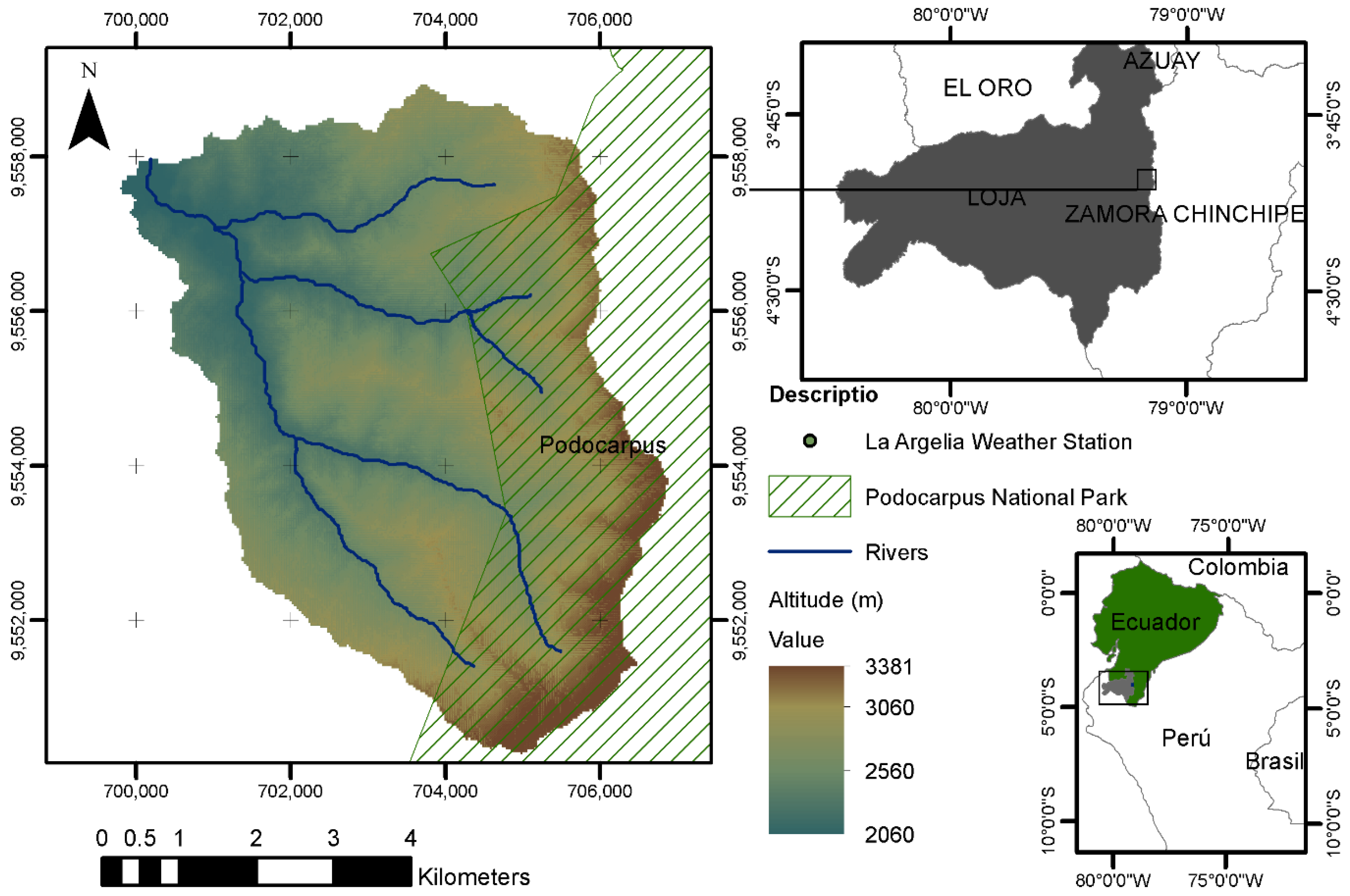
2.1. Study Area
2.2. Land Use/Land Cover Change (LUCC)
2.3. Hydric Recharge Estimation
2.4. Flash Flood Risk Assessment
2.5. Meteorological Forecast
2.6. Water Availability Estimation
3. Results
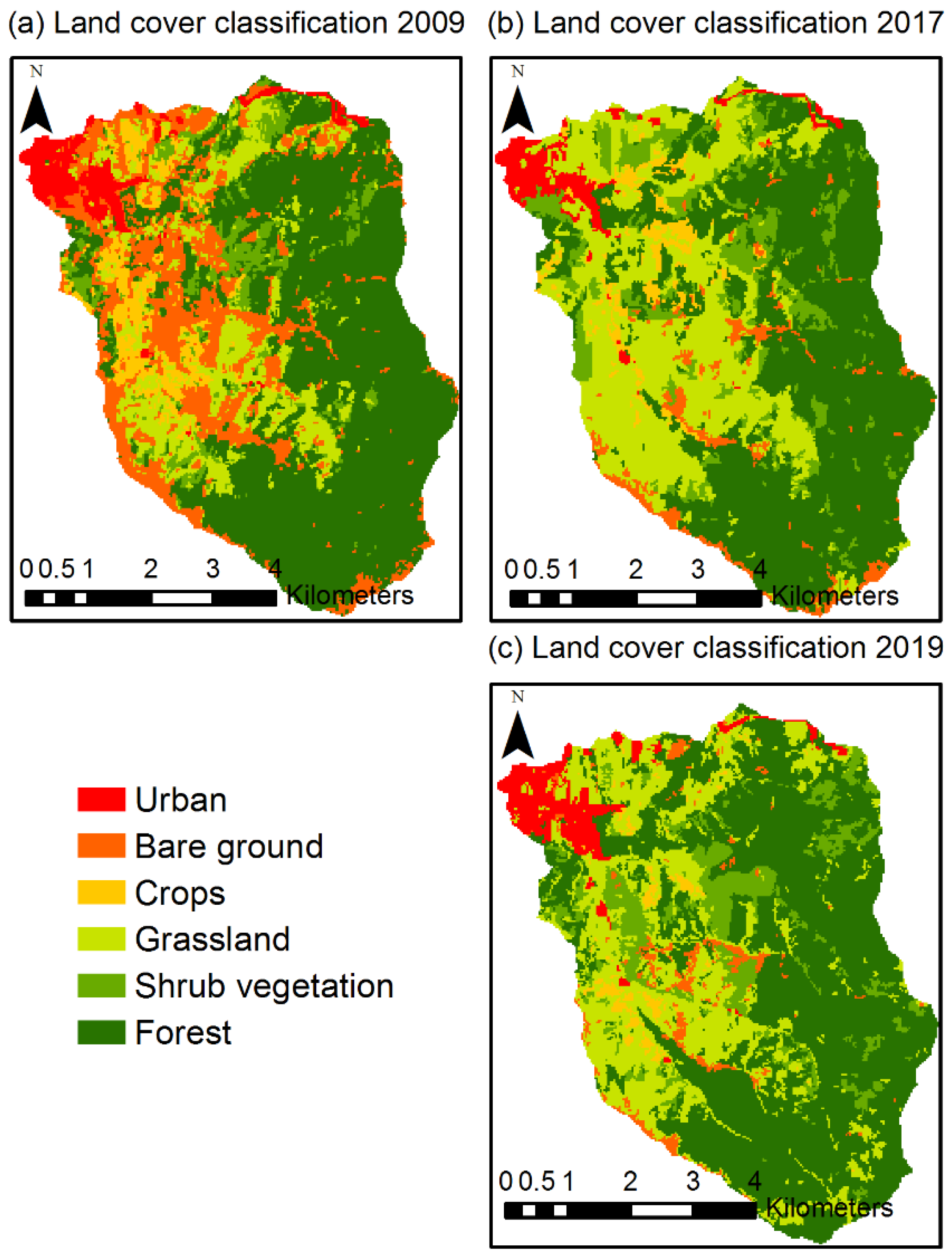
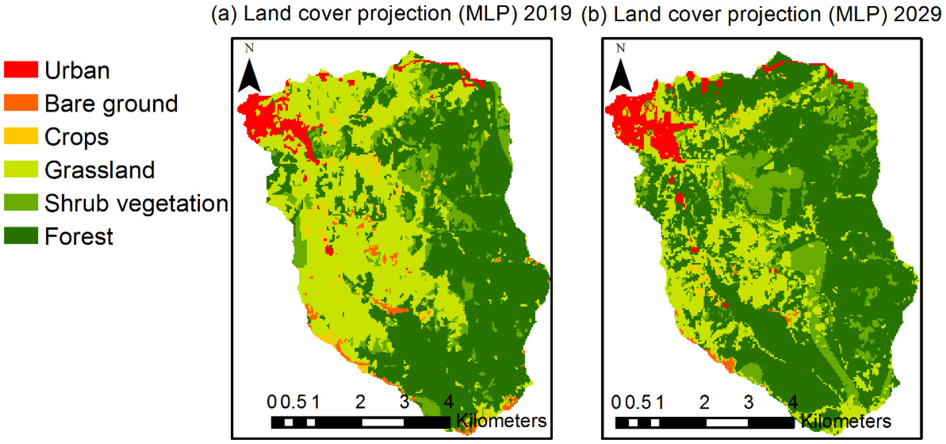
3.1. LULC and LUCC
3.2. Hydric Recharge Analysis
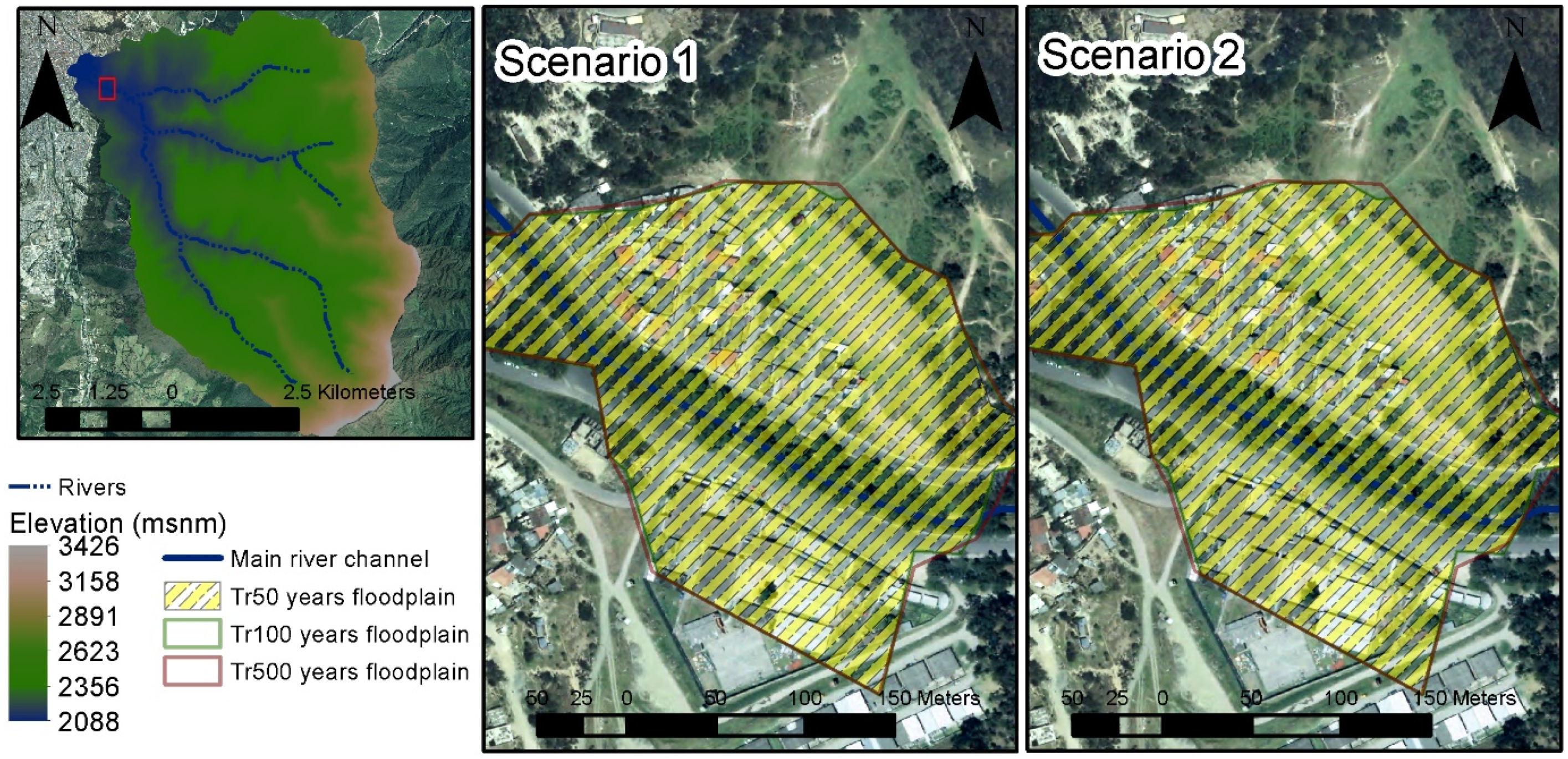
3.3. Floodplains
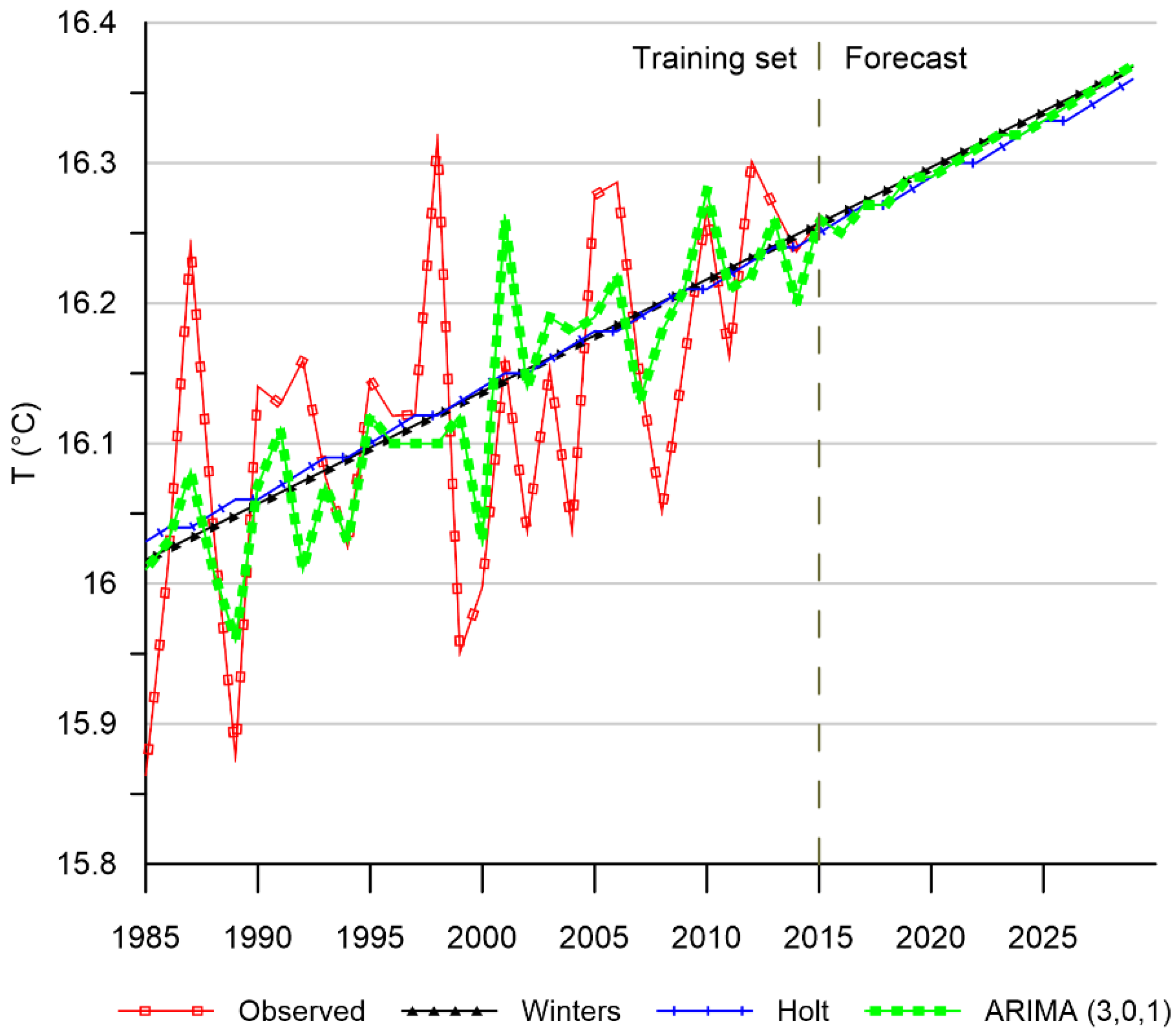
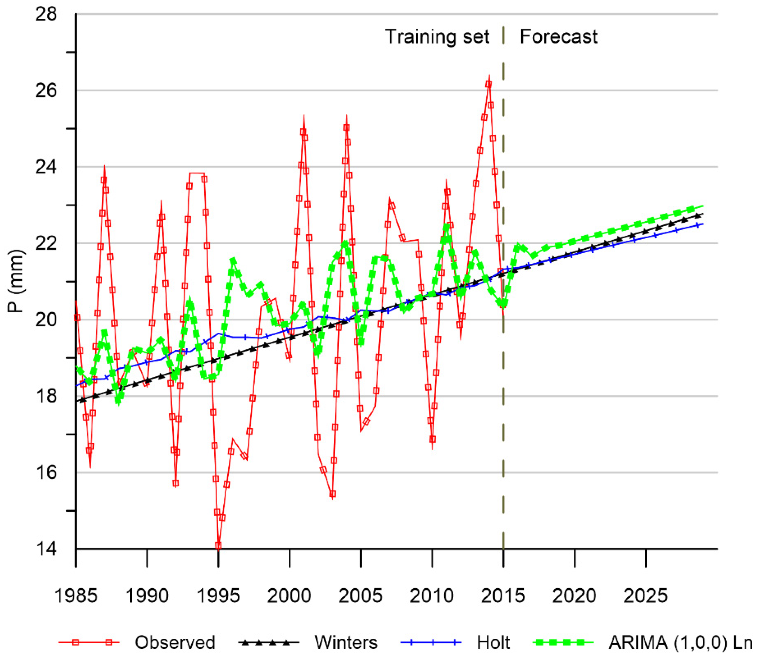
3.4. Meteorological Forecast
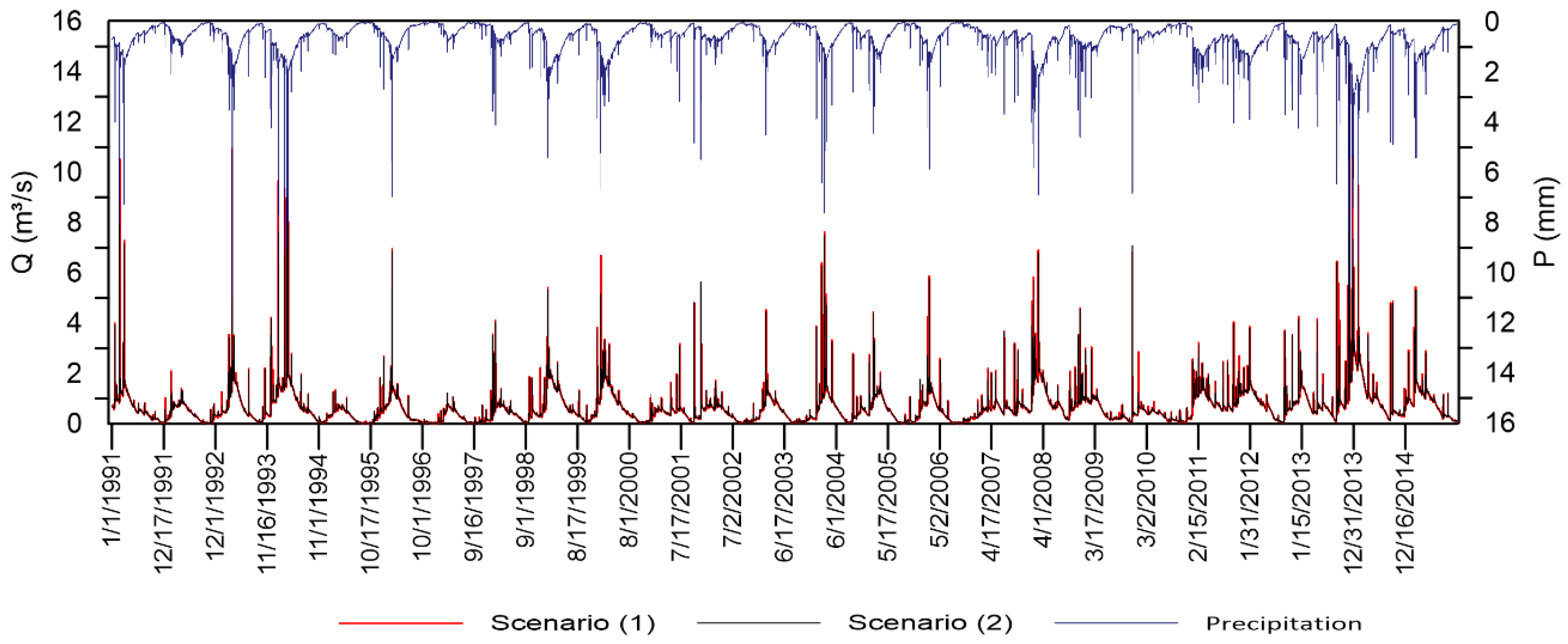
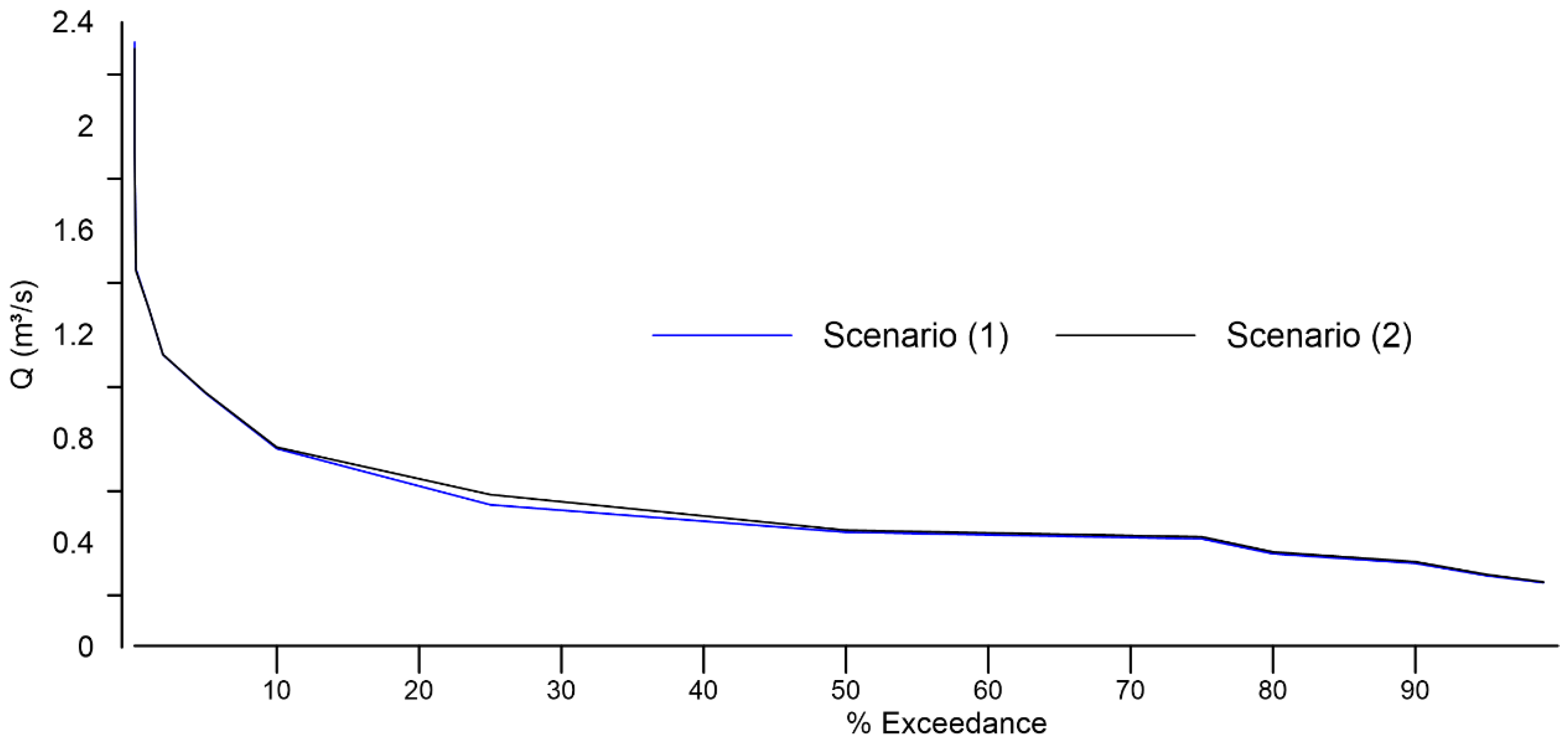
3.5. Basin Hydrological Response
4. Discussion
4.1. LULC and LUCC Analysis
4.2. Hydric Recharge Analysis
4.3. Floodplains Analysis
4.4. Meteorological Forecast Analysis
4.5. Basin Hydrological Response Analysis
4.6. Actual Context of the ZH Basin and the Need for IWRM
5. Conclusions
Supplementary Materials
Author Contributions
Funding
Institutional Review Board Statement
Informed Consent Statement
Data Availability Statement
Acknowledgments
Conflicts of Interest
References
- Boongaling, C.G.K.; Faustino-Eslava, D.V.; Lansigan, F.P. Modeling land use change impacts on hydrology and the use of landscape metrics as tools for watershed management: The case of an ungauged catchment in the Philippines. Land Use Policy 2018, 72, 116–128. [Google Scholar] [CrossRef]
- Ewunetu, A.; Simane, B.; Teferi, E.; Zaitchik, B.F. Land cover change in the blue nile river headwaters: Farmers’ perceptions, pressures, and satellite-based mapping. Land 2021, 10, 68. [Google Scholar] [CrossRef]
- Manzano, L.R.; Díaz, C.; Gómez, M.A.; Mastachi, C.A.; Soares, D. Use of structural systems analysis for the integrated water resources management in the Nenetzingo river watershed, Mexico. Land Use Policy 2019, 87, 2–11. [Google Scholar] [CrossRef]
- Baude, M.; Meyer, B.C.; Schindewolf, M. Land use change in an agricultural landscape causing degradation of soil based ecosystem services. Sci. Total Environ. 2019, 659, 1526–1536. [Google Scholar] [CrossRef] [PubMed]
- Delgado, A.M.; Pantoja, F. Structural analysis for the identification of key variables in the Ruta del Oro, Nariño Colombia. Dyna 2015, 82, 27–33. [Google Scholar] [CrossRef]
- Edwards, E.C.; Harter, T.; Fogg, G.E.; Washburn, B.; Hamad, H. Assessing the effectiveness of drywells as tools for stormwater management and aquifer recharge and their groundwater contamination potential. J. Hydrol. 2016, 539, 539–553. [Google Scholar] [CrossRef]
- Guerrero-Morales, J.; Fonseca, C.R.; Goméz-Albores, M.A.; Sampedro-Rosas, M.L.; Silva-Gómez, S.E. Proportional Variation of Potential Groundwater Recharge as a Result of Climate Change and Land-Use: A Study Case in Mexico. Land 2020, 9, 364. [Google Scholar] [CrossRef]
- Junker, M. Método RAS Para Determinar la Recarga de Agua Subterránea; Forgaes: San Salvador, El Salvador, 2005. [Google Scholar]
- Schosinsky, G.; Losilla, M. Modelo analítico para determinar la infiltración con base en la lluvia mensual. Rev. Geológica América Cent. 2000, 23, 43–55. [Google Scholar] [CrossRef]
- Schosinsky, G. Cálculo de la recarga potencial de acuíferos mediane un balance hídrico de suelos. Rev. Geológica América Cent. 2006, 34–35, 13–30. [Google Scholar]
- Golshan, M.; Jahanshahi, A.; Afzali, A. Flood hazard zoning using HEC-RAS in GIS environment and impact of manning roughness coefficient changes on flood zones in Semi-arid climate. Desert 2016, 21, 24–34. [Google Scholar] [CrossRef]
- Liu, J.; Shi, Z. wu Quantifying land-use change impacts on the dynamic evolution of flood vulnerability. Land Use Policy 2017, 65, 198–210. [Google Scholar] [CrossRef]
- Arteaga, J.; Ochoa, P.; Fries, A.; Boll, J. Identification of Priority Areas for Integrated Management of Semiarid Watersheds in the Ecuadorian Andes. JAWRA J. Am. Water Resour. Assoc. 2020, 56, 270–282. [Google Scholar] [CrossRef]
- Mararakanye, N.; Le Roux, J.J.; Franke, A.C. Using satellite-based weather data as input to SWAT in a data poor catchment. Phys. Chem. Earth 2020, 117, 102871. [Google Scholar] [CrossRef]
- Wilson, T.S.; Van Schmidt, N.D.; Langridge, R. Land-use change and future water demand in California’s Central Coast. Land 2020, 9, 322. [Google Scholar] [CrossRef]
- Oñate-Valdivieso, F.; Bosque Sendra, J. Semidistributed hydrological model with scarce information: Application to a large south american binational basin. J. Hydrol. Eng. 2014, 19, 1006–1014. [Google Scholar] [CrossRef]
- Aguado-Rodríguez, G.J.; Quevedo-Nolasco, A.; Castro-Popoca, M.; Arteaga-Ramírez, R.; Vázquez-Peña, M.A.; Zamora-Morales, B.P. Meteorological variables prediction through ARIMA models. Agrociencia 2016, 50, 1–13. [Google Scholar]
- Hossain, M.; Hasan, E.; Alauddin, M. The Variability of the Historical and Future Temperature in Bangladesh. Br. J. Appl. Sci. Technol. 2017, 20, 1–13. [Google Scholar] [CrossRef]
- Norouzi, M. Time Series Analysis on the Appropriate Time for Malaria Residual Spraying Based on Anopheles abundance, Temperature, and Precipitation between 2009–2016 in Kazerun, South of Iran. J. Health Sci. Surveill. Syst. 2018, 6, 99–105. [Google Scholar]
- Rodrigues, J.; Deshpande, A. Prediction of Rainfall for all the States of India Using Auto-Regressive Integrated Moving Average Model and Multiple Linear Regression. In Proceedings of the International Conference on Computing, Communication, Control and Automation, Pune, India, 17–18 August 2017; pp. 1–4. [Google Scholar] [CrossRef]
- Mora, D.E.; Campozano, L.; Cisneros, F.; Wyseure, G.; Willems, P. Climate changes of hydrometeorological and hydrological extremes in the Paute basin, Ecuadorean Andes. Hydrol. Earth Syst. Sci. 2014, 18, 631–648. [Google Scholar] [CrossRef]
- Buytaert, W.; Vuille, M.; Dewulf, A.; Urrutia, R.; Karmalkar, A.; Célleri, R. Uncertainties in climate change projections and regional downscaling in the tropical Andes: Implications for water resources management. Hydrol. Earth Syst. Sci. 2010, 14, 1247–1258. [Google Scholar] [CrossRef]
- Foragua Mecanismo Financiero FORAGUA. Available online: http://www.foragua.org/ (accessed on 29 April 2020).
- Mejía-Veintimilla, D.; Ochoa-Cueva, P.; Samaniego-Rojas, N.; Félix, R.; Arteaga, J.; Crespo, P.; Oñate-Valdivieso, F.; Fries, A. River Discharge Simulation in the High Andes of Southern Ecuador Using High-Resolution Radar Observations and Meteorological Station Data. Remote Sens. 2019, 11, 2804. [Google Scholar] [CrossRef]
- INAMHI Tipo de Climas. Available online: http://www.serviciometeorologico.gob.ec/geoinformacion-hidrometeorologica/ (accessed on 30 April 2020).
- Oñate-Valdivieso, F.; Uchuari, V.; Oñate-Paladines, A. Large-Scale Climate Variability Patterns and Drought: A Case of Study in South-America. Water Resour. Manag. 2020, 34, 2061–2079. [Google Scholar] [CrossRef]
- Ochoa-Cueva, P.; Fries, A.; Montesinos, P.; Rodríguez-Díaz, J.A.; Boll, J. Spatial Estimation of Soil Erosion Risk by Land-cover Change in the Andes OF Southern Ecuador. Land Degrad. Dev. 2015, 26, 565–573. [Google Scholar] [CrossRef]
- González-Jaramillo, V.; Fries, A.; Zeilinger, J.; Homeier, J.; Paladines-Benitez, J.; Bendix, J. Estimation of Above Ground Biomass in a Tropical Mountain Forest in Southern Ecuador Using Airborne LiDAR Data. Remote Sens. 2018, 10, 660. [Google Scholar] [CrossRef]
- Zarate, C. Hacia un Modelo de Ordenación Para los Territorios de Protección Natural del Área de Influencia Inmediata de la Ciudad de Loja. Microcuenca El Carmen; Universidad de Cuenca: Cuenca, Ecuador, 2011. [Google Scholar]
- Alvarez Bustamante, L. Disponibilidad y Demanda del Recurso Hídrico Superficial; Estudio de caso: Subcuenca Zamora Huayco, Ecuador, 2017. [Google Scholar]
- Hansen, M.C.; Loveland, T.R. A review of large area monitoring of land cover change using Landsat data. Remote Sens. Environ. 2012, 122, 66–74. [Google Scholar] [CrossRef]
- Pandžić, M.; Mihajlović, D.; Pandžić, J.; Pfeifer, N. Assessment of the geometric quality of sentinel-2 data. Int. Arch. Photogramm. Remote Sens. Spat. Inf. Sci. ISPRS Arch. 2016, 41, 489–494. [Google Scholar] [CrossRef]
- MAGAP Ortofoto. Available online: http://mapas.sigtierras.gob.ec/ortofoto/ (accessed on 1 March 2020).
- Congedo, L. Semi-Automatic Classification Plugin Documentation. Release 2016, 5, 268. [Google Scholar] [CrossRef]
- Fang, Y.; Zhao, J.; Liu, L.; Wang, J. Comparision of Eight Topographic Correction Algorithms Applied to Landsat-8 OLI Imagery Based on the DEM. In Proceedings of the IOP Conference Series: Earth and Environmental Science, Prague, Czech Republic, 7–11 September 2020; Volume 428. [Google Scholar] [CrossRef]
- Chuvieco, E. Teledetección Ambiental: La Observación de la Tierra Desde el Espacio; Tercera; Ariel Ciencia: Barcelona, Spain, 2007; ISBN 84-344-8047-6. [Google Scholar]
- Alaska Satellite Facility ALOS PALSAR Terrain-Corrected (RTC) DEM data. Available online: https://search.asf.alaska.edu/ (accessed on 14 May 2020).
- Mishra, V.; Rai, P.; Mohan, K. Prediction of land use changes based on land change modeler (LCM) using remote sensing: A case study of Muzaffarpur (Bihar), India. J. Geogr. Inst. Jovan Cvijic SASA 2014, 64, 111–127. [Google Scholar] [CrossRef]
- Hamdy, O.; Zhao, S.; Salheen, M.A.; Eid, Y.Y. Analyses the Driving Forces for Urban Growth by Using IDRISI®Selva Models Abouelreesh-Aswan as a Case Study. Int. J. Eng. Technol. 2017, 9, 226–232. [Google Scholar] [CrossRef]
- Khoi, D.D.; Murayama, Y. Forecasting areas vulnerable to forest conversion in the tam Dao National Park region, Vietnam. Remote Sens. 2010, 2, 1249–1272. [Google Scholar] [CrossRef]
- Foody, G.M. Explaining the unsuitability of the kappa coefficient in the assessment and comparison of the accuracy of thematic maps obtained by image classification. Remote Sens. Environ. 2020, 239, 111630. [Google Scholar] [CrossRef]
- Oñate-Valdivieso, F.; Bosque Sendra, J. Application of GIS and remote sensing techniques in generation of land use scenarios for hydrological modeling. J. Hydrol. 2010, 395, 256–263. [Google Scholar] [CrossRef]
- Zanetti, S.S.; Dohler, R.E.; Cecílio, R.A.; Pezzopane, J.E.M.; Xavier, A.C. Proposal for the use of daily thermal amplitude for the calibration of the Hargreaves-Samani equation. J. Hydrol. 2019, 571, 193–201. [Google Scholar] [CrossRef]
- Alam, M.S.; Lamb, D.W.; Rahman, M.M. A refined method for rapidly determining the relationship between canopy NDVI and the pasture evapotranspiration coefficient. Comput. Electron. Agric. 2018, 147, 12–17. [Google Scholar] [CrossRef]
- Pôças, I.; Calera, A.; Campos, I.; Cunha, M. Remote sensing for estimating and mapping single and basal crop coefficientes: A review on spectral vegetation indices approaches. Agric. Water Manag. 2020, 233, 106081. [Google Scholar] [CrossRef]
- Rubio, E.; Colin, J.; D’Urso, G.; Trezza, R.; Allen, R.; Calera, A.; González, J.; Jochum, A.; Menenti, M.; Tasumi, M.; et al. Golden day comparison of methods to retrieve et (Kc-NDVI, Kc-analytical, MSSEBS, METRIC). AIP Conf. Proc. 2006, 852, 193–200. [Google Scholar] [CrossRef]
- Toureiro, C.; Serralheiro, R.; Shahidian, S.; Sousa, A. Irrigation management with remote sensing: Evaluating irrigation requirement for maize under Mediterranean climate condition. Agric. Water Manag. 2017, 184, 211–220. [Google Scholar] [CrossRef]
- Fries, A.; Silva, K.; Pucha-Cofrep, F.; Oñate-Valdivieso, F.; Ochoa-Cueva, P. Water Balance and Soil Moisture Deficit of Different Vegetation Units under Semiarid Conditions in the Andes of Southern Ecuador. Climate 2020, 8, 30. [Google Scholar] [CrossRef]
- Nie, W.-B.; Li, Y.-B.; Liu, Y.; Ma, X.-Y. An Approximate Explicit Green-Ampt Infiltration Model for Cumulative Infiltration. Soil Sci. Soc. Am. J. 2018, 82, 919–930. [Google Scholar] [CrossRef]
- De Almeida, I.K.; Almeida, A.K.; Anache, J.A.A.; Steffen, J.L.; Alves Sobrinho, T. Estimation on time of concentration of overland flow in watersheds: A review. Geociencias 2014, 33, 661–671. [Google Scholar]
- Jin-Young, K.; Duk-Soon, K.; Deg-Hyo, B.; Hyun-Han, K. Bayesian parameter estimation of Clark unit hydrograph using multiple rainfall-runoff data. Korea Water Resour. Assoc. 2020, 53, 383–393. [Google Scholar] [CrossRef]
- Guachamanin, W.; García, F.; Arteaga, M.; Cadena, J. Determinación de Ecuaciones Para el Cálculo de Intensidades Máximas de Precipitación. Actualización del Estudio de Lluvias Intensas; INAMHI: Quito, Ecuador, 2019; Available online: http://https://www.serviciometeorologico.gob.ec/Publicaciones/Hidrologia (accessed on 17 May 2020).
- Bruland, O. How extreme can unit discharge become in steep Norwegian catchments? Hydrol. Res. 2020, 51, 290–307. [Google Scholar] [CrossRef]
- Arcement, G.J.; Schneider, V.R. Guide for Selecting Manning’s Roughness Coefficients for Natural Channels and Flood Plains; US Geological Survey Water Supply Paper 2339; U.S. Geological Survey: Virginia, VA, USA, 1989; pp. 28–31.
- Barnes, H.H. Roughness Characteristics of Natural Channels; US Geological Survey Water Supply Paper 1849; U.S. Geological Survey: Virginia, VA, USA, 1967; Volume 1, pp. 108–121.
- Bang, S.; Bishnoi, R.; Chauhan, A.S.; Dixit, A.K.; Chawla, I. Fuzzy Logic based Crop Yield Prediction using Temperature and Rainfall parameters predicted through ARMA, SARIMA, and ARMAX models. In Proceedings of the Twelfth International Conference on Contemporary Computing (IC3), Noida, India, 8–10 August 2019; pp. 1–6. [Google Scholar] [CrossRef]
- Liu, H.; Li, C.; Shao, Y.; Zhang, X.; Zhai, Z.; Wang, X.; Qi, X.; Wang, J.; Hao, Y.; Wu, Q.; et al. Forecast of the trend in incidence of acute hemorrhagic conjunctivitis in China from 2011–2019 using the Seasonal Autoregressive Integrated Moving Average (SARIMA) and Exponential Smoothing (ETS) models. J. Infect. Public Health 2020, 13, 287–294. [Google Scholar] [CrossRef] [PubMed]
- Dhamodharavadhani, S.; Rathipriya, R. Region-Wise Rainfall Prediction Using MapReduce-Based Exponential Smoothing Techniques. In Advances in Big Data and Cloud Computing; Springer: Singapore, 2019; pp. 229–239. [Google Scholar]
- Essenfelder, A.H. SWAT Weather Database: A Quick Guide; Version: V.0.16.06. 2016. Available online: https://www.researchgate.net/profile/Arthur-Hrast-Essenfelder-2/publication/330221011_SWAT_Weather_Database_A_Quick_Guide/links/5c34a39192851c22a363cbb0/SWAT-Weather-Database-A-Quick-Guide.pdf (accessed on 29 April 2020).
- Arnold, J.G.; Kiniry, J.R.; Srinivasan, R.; Williams, J.R.; Haney, E.B.; Neitsch, S.L. Input/Output Documentation Soil & Water Assessment Tool; Texas Water Resources Institute: Texas, TX, USA, 2012. [Google Scholar]
- Kalcic, M.M.; Chaubey, I.; Frankenberger, J. Defining Soil and Water Assessment Tool (SWAT) hydrologic response units (HRUs) by field boundaries. Int. J. Agric. Biol. Eng. 2015, 8, 1–12. [Google Scholar] [CrossRef]
- Izabá-Ruiz, R.; García, D. Estimación de la diponibilidad hídrica superficial en la microcuenca del río Mapachá, San Lorenzo, Boaco. Agua Conoc. 2018, 3, 1–22. [Google Scholar]
- Müller, M.F.; Thompson, S.E. Comparing statistical and process-based flow duration curve models in ungauged basins and changing rain regimes. Hydrol. Earth Syst. Sci. 2016, 20, 669–683. [Google Scholar] [CrossRef]
- Zhang, Y.; Singh, V.P.; Byrd, A.R. Entropy parameter M in modeling a flow duration curve. Entropy 2017, 19, 654. [Google Scholar] [CrossRef]
- Eastman, J.R. Guide to GIS and Image Processing; IDRISI Production, Ed.; Clark University: Worcester, MA, USA, 2006. [Google Scholar]
- Roy, H.G.; Fox, D.M.; Emsellem, K. Predicting land cover change in a Mediterranean catchment at different time scales. In Proceedings of the International Conference on Computational Science and Its Applications, Guimarães, Portugal, 30 June–3 July 2014; Volume 8582 LNCS, pp. 315–330. [Google Scholar] [CrossRef]
- López, J.; Cruz, B. Dinámica forestal y uso de suelo en las cuencas que integran al municipio Tomatlán, Jalisco. Rev. Mex. Cienc. For. 2020, 11, 47–68. [Google Scholar] [CrossRef][Green Version]
- Landis, J.R.; Koch, G.G. Landis amd Koch1977_agreement of categorical data. Biometrics 1977, 33, 159–174. [Google Scholar] [CrossRef]
- Fleiss, J.L.; Levin, B.; Cho Paik, M. Statistical Methods for Rates and Proportions; John Wiley & Sons: Hoboken, NJ, USA, 2013. [Google Scholar]
- Monserud, R.A.; Leemans, R. Comparing global vegetation maps with the Kappa statistic. Ecol. Model. 1992, 62, 275–293. [Google Scholar] [CrossRef]
- Serrano, J.A. Estimación de la Relación de Lluvia “R” Para la Determinación de las Curvas de Intensidad-Duración-Frecuencia en la Provincia de de Loja-Ecuador con Escasa o nula Información Pluviográfica; Universidad Nacional Autónoma de México: Mexico City, Mexico, 2011. [Google Scholar]
- Muñoz, P.; Orellana-Alvear, J.; Willems, P.; Célleri, R. Flash-flood forecasting in an andean mountain catchment-development of a step-wise methodology based on the random forest algorithm. Water 2018, 10, 1519. [Google Scholar] [CrossRef]
- Camici, S.; Tarpanelli, A.; Brocca, L.; Melone, F.; Moramarco, T. Design soil moisture estimation by comparing continuous and storm-based rainfall-runoff modeling. Water Resour. Res. 2011, 47, 1–18. [Google Scholar] [CrossRef]
- Morán-Tejeda, E.; Bazo, J.; López-Moreno, J.I.; Aguilar, E.; Azorín-Molina, C.; Sanchez-Lorenzo, A.; Martínez, R.; Nieto, J.J.; Mejía, R.; Martín-Hernández, N.; et al. Climate trends and variability in Ecuador (1966–2011). Int. J. Climatol. 2016, 36, 3839–3855. [Google Scholar] [CrossRef]
- INEC Población y Tasas de Crecimeinto Intercensal de 2010—2001—1990 por Sexo Según Parroquias. Available online: https://www.ecuadorencifras.gob.ec (accessed on 1 July 2020).
- Yang, M.; Mou, Y.; Meng, Y.; Liu, S.; Peng, C.; Zhou, X. Modeling the effects of precipitation and temperature patterns on agricultural drought in China from 1949 to 2015. Sci. Total Environ. 2020, 711, 135139. [Google Scholar] [CrossRef]
- Fries, A.E. Climate change. In Management of Hydrological Systems; CRC Press: Boca Raton, FL, USA, 2020; pp. 97–112. [Google Scholar]
- Crespo, P.; Celleri, R.; Buytaert, W.; Feyen, J.A.N.; Iñiguez, V.; Borja, P.; Bievre, B.D.E.; Cuenca, U. De Land use change impacts on the hydrology of wet Andean páramo ecosystems. In Status and Perspectives of Hydrology in Small Basins; IAHS Press: Goslar-Hahnenklee, Germany, 2010; pp. 71–76. [Google Scholar]
- Chamba-Ontaneda, M.; Massa-Sánchez, P.; Fries, A. Presión demográfica sobre el agua: Un análisis regional. Rev. Geogr. Venez. 2019, 60, 360–377. [Google Scholar]
- Benavides Muñoz, H.M.; Zari, J.E.A.; Fries, A.E.; Sánchez-Paladines, J.; Gallegos Reina, A.J.; Hernández-Ocampo, R.V.; Ochoa Cueva, P. Management of Hydrological Systems; CRC Press: Boca Raton, FL, USA, 2020; ISBN 9781003024576. [Google Scholar]


| Coverage | 2019 | 2029 |
|---|---|---|
| Forest | 54.81 | 58.72 |
| Shrub vegetation | 11.02 | 13.71 |
| Grassland | 25.72 | 22.45 |
| Crops | 1.63 | 0.64 |
| Bare soil | 2.8 | 0.45 |
| Urban | 4.03 | 4.03 |
| Distribution Functions | Accumulated Error | NSE | RSME |
|---|---|---|---|
| Gamma 2 parameters | 8.754 | 0.99 | 1.21 |
| Pearson Type III | 168.38 | −3.33 | 25.77 |
| Exponential | 195.86 | −4.86 | 27.16 |
| Nash | 10.70 | 0.98 | 1.63 |
| Normal | 11.33 | 0.98 | 2.20 |
| LogNormal | 9.19 | 0.99 | 1.27 |
| Gumbel | 12.42 | 0.97 | 1.72 |
| Tr (Years) | 50 | 100 | 500 |
|---|---|---|---|
| P 24 h (mm) | 69.04 | 73.38 | 82.72 |
| I Tc (mm/h) | 16.24 | 17.26 | 19.46 |
| 2019 Q (m3/s) | 3.59 | 5.29 | 9.92 |
| 2029 Q (m3/s) | 3.00 | 4.55 | 8.87 |
| Scenario | Tr (Years) | Flooding-Susceptible Areas (ha) | Floodplain Margin (m) | d (m) | v (m/s) |
|---|---|---|---|---|---|
| 2019 | 50 | 28.80 | 33.46 | 1.53 | 0.41 |
| 100 | 29.47 | 33.47 | 1.87 | 0.45 | |
| 500 | 30.86 | 35.65 | 2.05 | 0.58 | |
| 2029 | 50 | 28.67 | 33.42 | 1.42 | 0.39 |
| 100 | 29.29 | 33.45 | 1.61 | 0.44 | |
| 500 | 30.65 | 35.64 | 1.97 | 0.56 |
| Variable | Model | Transformation | R2 | RMSE | MAE |
|---|---|---|---|---|---|
| T average | ARIMA (3,0,1) | None | 0.44 | 0.09 | 0.06 |
| T average | WINTERS | None | 0.32 | 0.08 | 0.06 |
| T average | HOLT | None | 0.30 | 0.10 | 0.07 |
| Variable | Model | Transformation | R2 | RMSE | MAE |
|---|---|---|---|---|---|
| Pmax average | ARIMA (1,0,0) | Natural logarithm | 0.12 | 3.31 | 2.63 |
| Pmax average | WINTERS | None | 0.06 | 2.93 | 2.67 |
| Pmax average | HOLT | None | 0.02 | 3.46 | 2.91 |
Publisher’s Note: MDPI stays neutral with regard to jurisdictional claims in published maps and institutional affiliations. |
© 2021 by the authors. Licensee MDPI, Basel, Switzerland. This article is an open access article distributed under the terms and conditions of the Creative Commons Attribution (CC BY) license (https://creativecommons.org/licenses/by/4.0/).
Share and Cite
Mera-Parra, C.; Oñate-Valdivieso, F.; Massa-Sánchez, P.; Ochoa-Cueva, P. Establishment of the Baseline for the IWRM in the Ecuadorian Andean Basins: Land Use Change, Water Recharge, Meteorological Forecast and Hydrological Modeling. Land 2021, 10, 513. https://doi.org/10.3390/land10050513
Mera-Parra C, Oñate-Valdivieso F, Massa-Sánchez P, Ochoa-Cueva P. Establishment of the Baseline for the IWRM in the Ecuadorian Andean Basins: Land Use Change, Water Recharge, Meteorological Forecast and Hydrological Modeling. Land. 2021; 10(5):513. https://doi.org/10.3390/land10050513
Chicago/Turabian StyleMera-Parra, Christian, Fernando Oñate-Valdivieso, Priscilla Massa-Sánchez, and Pablo Ochoa-Cueva. 2021. "Establishment of the Baseline for the IWRM in the Ecuadorian Andean Basins: Land Use Change, Water Recharge, Meteorological Forecast and Hydrological Modeling" Land 10, no. 5: 513. https://doi.org/10.3390/land10050513
APA StyleMera-Parra, C., Oñate-Valdivieso, F., Massa-Sánchez, P., & Ochoa-Cueva, P. (2021). Establishment of the Baseline for the IWRM in the Ecuadorian Andean Basins: Land Use Change, Water Recharge, Meteorological Forecast and Hydrological Modeling. Land, 10(5), 513. https://doi.org/10.3390/land10050513