Local Climate Zone Mapping Using Multi-Source Free Available Datasets on Google Earth Engine Platform

Abstract

As one of the widely concerned urban climate issues, urban heat island (UHI) has been studied using the local climate zone (LCZ) classification scheme in recent years. More and more effort has been focused on improving LCZ mapping accuracy. It has become a prevalent trend to take advantage of multi-source images in LCZ mapping. To this end, this paper tried to utilize multi-source freely available datasets: Sentinel-2 multispectral instrument (MSI), Sentinel-1 synthetic aperture radar (SAR), Luojia1-01 nighttime light (NTL), and Open Street Map (OSM) datasets to produce the 10 m LCZ classification result using Google Earth Engine (GEE) platform. Additionally, the derived datasets of Sentinel-2 MSI data were also exploited in LCZ classification, such as spectral indexes (SI) and gray-level co-occurrence matrix (GLCM) datasets. The different dataset combinations were designed to evaluate the particular dataset’s contribution to LCZ classification. It was found that: (1) The synergistic use of Sentinel-2 MSI and Sentinel-1 SAR data can improve the accuracy of LCZ classification; (2) The multi-seasonal information of Sentinel data also has a good contribution to LCZ classification; (3) OSM, GLCM, SI, and NTL datasets have some positive contribution to LCZ classification when individually adding them to the seasonal Sentinel-1 and Sentinel-2 datasets; (4) It is not an absolute right way to improve LCZ classification accuracy by combining as many datasets as possible. With the help of the GEE, this study provides the potential to generate more accurate LCZ mapping on a large scale, which is significant for urban development.

1. Introduction

As increasing people live in cities, the greatest public health challenges of the 21st-century will come from cities. Therefore, human health is likely to be especially vulnerable to the adverse effects of urban climate change. As one of the widely concerned urban climate issues, urban heat island (UHI) is a universal phenomenon that occurs in cities worldwide [1,2,3]. It has caused some urban climate problems, such as heatwaves and air pollution [4,5,6,7] and has widely aroused people’s attention in the world [8]. In the past several decades, it has been the preoccupation of researchers to measure the UHI effect by comparing the temperature of “urban” and “rural” areas. However, the simple division of “urban” and “rural” areas is always based on the researchers’ experience and lacks a unified standard.

Stewart and Oke (2012) proposed a local climate zone (LCZ) classification scheme, which provides a research framework for UHI studies and standardizes the worldwide exchange of urban temperature observation [9]. There are 17 LCZ classes in the LCZ classification scheme (

Table 1. Local climate zones scheme [9].

Built Type	Definition	Land Cover Type	Definition
1. Compact high-rise	Dense mix of tall buildings to tens of stories. Few or no trees. Land cover mostly paved. Concrete, steel, stone, and glass construction materials.	A. Dense trees	Heavily wooded landscape of deciduous and/or evergreen trees. Land cover mostly pervious (low plants). Zone function is natural forest, tree cultivation, or urban park.
2. Compact midrise	Dense mix of midrise buildings (3–9 stories). Few or no trees. Land cover mostly paved. Stone, brick, tile, and concrete construction materials.	B. Scattered trees	Lightly wooded landscape of deciduous and/or evergreen trees. Land cover mostly pervious (low plants). Zone function is natural forest, tree cultivation, or urban park.
3. Compact low-rise	Dense mix of low-rise buildings (1–3 stories). Few or no trees. Land cover mostly paved. Stone, brick, tile, and concrete construction materials.	C. Bush, scrub	Open arrangement of bushes, shrubs, and short, woody trees. Land cover mostly pervious (bare soil or sand). Zone function is natural scrubland or agriculture.
4. Open high-rise	Open arrangement of tall buildings to tens of stories. Abundance of pervious land cover (low plants, scattered trees). Concrete, steel, stone, and glass construction materials.	D. Low plants	Featureless landscape of grass or herbaceous plants/crops. Few or no trees. Zone function is natural grassland, agriculture, or urban park.
5. Open midrise	Open arrangement of midrise buildings (3–9 stories). Abundance of pervious land cover (low plants, scattered trees). Concrete, steel, stone, and glass construction materials.	E. Bare rock or paved	Featureless landscape of rock or paved cover. Few or no trees or plants. Zone function is natural desert (rock) or urban transportation.
6. Open low-rise	Open arrangement of low-rise buildings (1–3 stories). Abundance of pervious land cover (low plants, scattered trees). Wood, brick, stone, tile, and concrete construction materials.	F. Bare soil or sand	Featureless landscape of soil or sand cover. Few or no trees or plants. Zone function is natural desert or agriculture.
7. Lightweight low-rise	Dense mix of single-story buildings. Few or no trees. Land cover mostly hard-packed. Lightweight construction materials (e.g., wood, thatch, corrugated metal).	G. Water	Large, open water bodies such as seas and lakes, or small bodies such as rivers, reservoirs, and lagoons.
8. Large low-rise	Open arrangement of large low-rise buildings (1–3 stories). Few or no trees. Land cover mostly paved. Steel, concrete, metal, and stone construction materials
9. Sparsely built	Sparse arrangement of small or medium-sized buildings in a natural setting. Abundance of pervious land cover (low plants, scattered trees).
10. Heavy industry	Low-rise and midrise industrial structures (towers, tanks, stacks). Few or no trees. Land cover mostly paved or hard-packed. Metal, steel, and concrete construction materials.

Source: Stewart and Oke (2012). ©American Meteorological Society. Used with permission.

): 10 built type classes (LCZ 1 to LCZ 10) and 7 land cover classes (LCZ A to LCZ G). LCZ provides a novel classification scheme to conduct UHI studies, in which urban landscapes are classified into different LCZ classes according to urban structures, land cover, and construction materials [9]. Hence, accurate LCZ classification information is important for UHI research.

The World Urban Database and Access Portal Tools (WUDAPT) were developed in 2015 as a community-based concept to generate a global database of LCZ information. WUDAPT generates LCZ maps of cities with the use of freely available Landsat data [10,11]. The WUDAPT method resamples the Landsat image of each city into a 100 m resolution to get the spectral information of local-scale urban structures [12]. Local experts with deep knowledge of individual cities build LCZ reference polygons using high-resolution google earth images. These polygons are converted into 100 m resolution pixels and used for training and testing LCZ classification models with Landsat images. The random forest (RF) and a rule-based machine learning approach are used for LCZ classification. The LCZ maps of Europe, Continental United States have been shared through the WUDAPT portal (http://www.wudapt.org accessed on 18 April 2021).

With the fast development of remote sensor technologies mounted on either airborne or spaceborne platforms, remote sensing data are also used for LCZ mapping. Based on the standard production of the WUDAPT project, Landsat data have become the most popular data in LCZ mapping [13,14,15,16,17,18,19]. However, the LCZ classification scheme includes so many classes, and the single data source has some limitations in distinguishing such many LCZ classes.

Now, it has become a prevalent trend in LCZ classification to take advantage of all kinds of datasets to produce a more accurate classification result. These datasets are complementary and combined for LCZ mapping. The dataset combination methods could be categorized into two types: (1) single-source datasets combination method. This method combines only one dataset and the derived datasets. The commonly used derived datasets are the contextual information and spectral indexes information. Some researchers tried to generate contextual information to further improve LCZ classification, such as grey-level co-occurrence matrix (GLCM), mean, minimum, maximum, median, and 25th and 75th quantile values derived from the spectral information of neighboring pixels [13,20,21,22]. Spectral indexes (SI) are also used to improved LCZ classification accuracy, such as normalized difference vegetation index (NDVI) and modified normalized difference water index (MNDWI) [23]. (2) Multi-source datasets combination method. This method combines different datasets, such as Landsat, Sentinel-1, Sentinel-2, Aster, National Polar-orbiting Partnership Visible Infrared Imager Radiometer Suite Nighttime Light, Global Urban Footprint, and Open Street Map (OSM) datasets [22,23,24,25,26,27].

Among all open-access remote sensing datasets, Sentinel-2 Multispectral instrument (MSI) and Sentinel-1 synthetic aperture radar (SAR) data are outstanding because of their relatively high spatial resolution (i.e., 10 m). Given that the difference in image mechanism between SAR and multispectral data, researchers have demonstrated that the synergetic use of Sentinel-2 MSI and Sentinel-1 SAR data can complement each other in the remote sensing image classification, such as soil moisture mapping [28], crop classification [29], glacial lake mapping [30] and wetlands mapping [31]. Several studies have demonstrated the potential to combine Sentinel-2 or Sentinel-1 data with other datasets on local climate zone classification to improve the limitation of a single dataset. However, few studies exist to date that the synergetic use of Sentinel-2 MSI and Sentinel-1 SAR data’s contribution on LCZ classification.

A variety of dataset combinations will lead to a large number of calculations for computers. Computer performance has been given more and more advanced requirements. Accordingly, Google Earth Engine (GEE) came into being and made it possible to process the huge quantity of remote sensing data in a computer that can open the website https://code.earthengine.google.com/ accessed on 31 March 2021. GEE is a cloud-based platform for planetary-scale geospatial analysis [32]. It contains a multi-petabyte catalog of satellite imagery and geospatial datasets. Therefore, the GEE platform is well-suited for dealing with various dataset combinations in LCZ mapping.

This paper aims to generate LCZ classification from multi-source free available datasets using the GEE platform, especially to analyze the attribution of different datasets to LCZ classification and find the best data combination in LCZ mapping of Wuhan.

2. Study Area and Datasets

Wuhan, the capital of central Hubei province, is located in central China. It is known as one of China’s “furnace cities” where summertime temperatures can soar to 40 °C. In the past several decades, Wuhan has experienced rapid urbanization, which would intensify the UHI effect. Additionally, the permanent resident population of Wuhan has reached 11.21 million. The increasingly serious urban heat island effect will affect the health of citizens. Therefore, Wuhan was selected as the study area (Figure 1).

2.1. Datasets Used for LCZ Mapping

Multi-source free available datasets were used in this study: Sentinel-2 MSI, Sentinel-1 SAR, Luojia1-01 nighttime light (NTL), and Open Street Map (OSM) dataset. Additionally, the derived datasets of Sentinel-2 MSI data were also exploited in LCZ classification, such as spectral indexes and GLCM datasets. All data processing procedures were realized in the GEE platform. GEE platform only contained Sentinel-2 MSI and Sentinel-1 SAR datasets. The Luojia1-01 NTL and OSM datasets were uploaded to the GEE platform for use.

Attention focused on datasets that might be complementary and so, when combined, provide an enhanced capacity to map the LCZ classes accurately. The combination of optical and radar remote sensing imagery provides complementary information which could improve the land cover classification accuracy [33,34]. Therefore, this study employed Sentinel-2 MSI and Sentinel-1 SAR data to improve the accuracy of LCZ mapping. Additionally, seasonal information can be used to increase the accuracy of LCZ classification [35]. The seasonal information Sentinel-2 MSI and Sentinel-1 SAR data were also generated in this study. The study period from 1 March 2018 to 28 February 2019 covers four seasons: spring (1 March to 31 May), summer (1 June to 31 August), autumn (1 September to 30 November), and winter (1 December to the next 28 February).

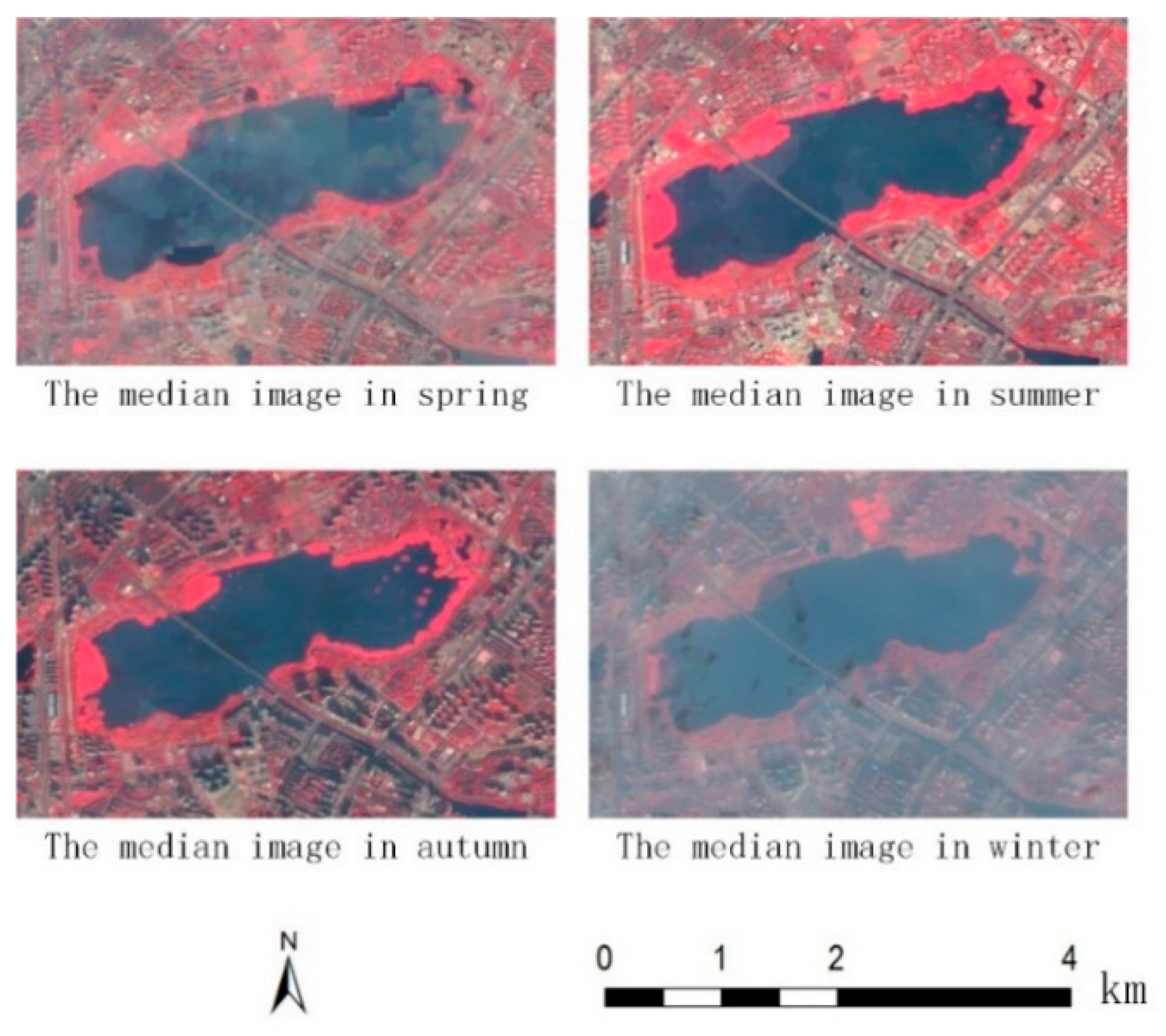
2.1.1. Sentinel-2 Data

Data from the Sentinel-2 MSI are provided by the European Space Agency. The MSI sensors provide relatively fine spatial resolution multispectral imagery globally at a high revisit time (5 days at the Equator with two satellites in orbit). Data are acquired in 13 spectral bands in the optical NIR, SWIR parts of the electromagnetic spectrum. The data are acquired at a range of spatial resolutions: four bands at 10 m, six bands at 20 m, and three bands at 60 m. Only the bands that acquired data with a 10 m spatial resolution (i.e., B2, B3, B4, and B8) were used. In the GEE platform, the dataset “Sentinel-2 MSI: MultiSpectral Instrument, Level-1C” was selected for use in this study. Only images with less than 10% cloud coverage were selected, and the clouds were masked using the Fmask method [36]. One hundred thirty-six images met the less than 10% cloud coverage condition. As the median value image can generate the equally high accuracy as time-series images [37], this study also calculated the annual and seasonal median value images. Figure 2 shows the seasonal Sentinel-2 median images. It can be found that the vegetation distribution has some difference in a different season, and the quality of the median image is worst in winter. The median image was covered with thin clouds in winter because the weather in winter is often hazy in Wuhan.

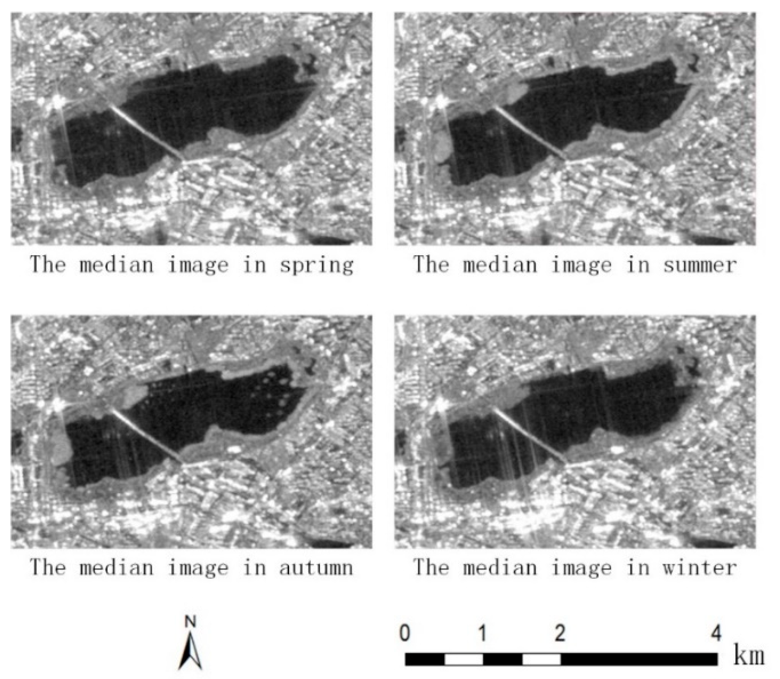
2.1.2. Sentinel-1 Data

Sentinel-1 SAR data acquired in the Interferometric Wide swath mode were used. These data represent the dual-polarized (VV and VH polarizations) response in C-band. Specifically, in the GEE platform, the dataset “Sentinel-1 SAR GRD: C-band synthetic aperture radar ground range detected, log scaling” was selected for use. Here, the Level-1 GRD products with a 10 m spatial resolution used. In total, 118 Sentinel-1 images were used to calculate the median value for the entire year. As with the Sentinel-2 data, the annual and seasonal median value images were calculated in the study. From Figure 3, the quality of median value images in the four seasons is good and slightly different from each other, which indicates that the quality of SAR images is not affected by weather by comparison with the multispectral image (i.e., Figure 2).

2.1.3. Spectral Indexes Data

A set of spectral indexes were derived from the Sentinel-2 data. The indices used were the NDVI [38] and NDWI [39]. As with the Sentinel-2 data, the median value for each pixel was used to form yearly and seasonal variables for use in the analyses. The equations of NDVI and NDWI are as follows:

$$\mathrm{NDVI}=\frac{{\rho }_{NIR}-{\rho }_{Red}}{{\rho }_{NIR}+{\rho }_{Red}}$$

(1)

$$\mathrm{NDWI}=\frac{{\rho }_{Green}-{\rho }_{NIR}}{{\rho }_{Green}+{\rho }_{NIR}}$$

(2)

${\rho }_{Green }$, ${\rho }_{Red }$, ${\rho }_{NIR}$ represent the B3, B4, and B8 bands of Sentinel-2 data, respectively.

2.1.4. Texture Data

Image textural information can be used to enhance image classification accuracy. Here, the texture was quantified using the GLCM approach [40,41]. The latter can be used to estimate a range of textural descriptors, and here 8 of them were used: contrast (Con), correlation (Corr), entropy (Ent), angular second moment (Asm), dissimilarity (Diss), inverse difference moment (Idm), sum average (Savg) and variance (Var). As the seasonal Sentinel-2 dataset had 16 bands and every band would correspond to 8 kinds of GLCM variables, 128 (16 × 8) GLCM variables were generated. To keep the maximum amount of information and the minimum data redundancy, a principal component analysis was applied to every kind of GLCM variable. The first principal component, which explained the largest proportion of this kind of variable, could be used as a single textural dataset in analyses. The textural dataset only included 8 kinds of first principal components of GLCM variables.

2.1.5. OSM Data

OSM is a free and editable map of the whole world [42] and can be downloaded from the website https://download.geofabrik.de/ accessed on 1 October 2019. Here, three OSM layers were used: building, water, and road (Figure 4). OSM data were uploaded to the GEE platform. OSM data were rasterized to a 10 m spatial resolution using bilinear interpolation.

2.1.6. NTL Data

The NTL dataset represents the visible light emerging from the Earth at night, and this is strongly related to variables such as urban density. Here, NTL data acquired by the Luojia1-01 satellite system were used (Figure 5). This system was launched in June 2018 and had a spatial resolution of 130 m [43]. Only one image was used. This was acquired on 13 June 2018 after the visual check of images at the website http://59.175.109.173:8888/index.html accessed on 1 October 2019. Then the Luojia1-01 data were uploaded to the GEE platform. To aid the integration of the data with the Sentinel datasets, the Luojia1-01 data were resampled to 10 m using the bilinear interpolation method in the GEE platform.

2.1.7. Datasets Combinations

A core thrust of the research was to explore the value of combining different datasets for LCZ mapping. Here, two broad categories of the dataset were available (

Table 2. The used datasets in this study.

Dataset Category	Dataset Name	Dataset Description	Bands Name	Feature Size
Sentinel datasets	S2_year	The median of all qualified Sentinel-2 images in 2018	B2, B3, B4, B8	4
	S1_year	The median of all Sentinel-1 images in 2018	VV, VH	2
	S2_season	The median of qualified Sentinel-2 images for each season in 2018	B2, B3, B4, B8	16 (4 × 4)
	S1_season	The median of Sentinel-1 images for each season in 2018	VV, VH	8 (2 × 4)
Secondary datasets	SI	The spectral indexes of the “S2_season” dataset	NDVI, NDWI	8 (2 × 4)
	GLCM(PC1)	The texture information of the “S2_season” dataset	Con, Corr, Var, Ent, Asm, Diss, Idm, Savg	8
	NTL	Luojia1-01 dataset	Band_ntl	1
	OSM	Open street map dataset	Building, Water, Road	3

). First, there are the original Sentinel-based datasets (Section 2.1.1 and Section 2.1.2). These two datasets are available on an annual and seasonal basis. In total, therefore, there are 4 Sentinel datasets (annual and seasonal data from Sentinel-1 and Sentinel-2). Second, there are four secondary datasets. The latter comprise the OSM, NTL, SI, and GLCM. These various datasets may be combined to enhance LCZ class separability and hence the accuracy with which LCZ classes may be mapped.

The datasets formed (Table 1) could be combined in various ways. Here, attention focused on a range of incremental combinations (

Table 3. The datasets in this study.

No.	Combination Name	Description
1	S2_year	This combination only includes” S2_year”
2	S2_S1_year	The combination of “S2_year” and “S1_year”
3	S2_season	This combination only includes” S2_ season”
4	S2_S1_season	This combination of “S2_season” and “S1_ season (median)”, taking this one as a basic combination.
5	+NTL	Adding any one secondary datasets to the basic combination
6	+SI
7	+OSM
8	+GLCM(PC1)
9	+GLCM(PC1)+NTL	Adding any two secondary datasets to the basic combination
10	+GLCM(PC1)+OSM
11	+OSM+NTL
12	+SI+ GLCM(PC1)
13	+SI+NTL
14	+SI+OSM
15	+NTL+OSM+GLCM(PC1)	Adding any three secondary datasets to the basic combination
16	+NTL+OSM+SI
17	+NTL+GLCM(PC1)+SI
18	+OSM+GLCM(PC1)+SI
19	+NTL+OSM+GLCM(PC1)+SI	Adding all secondary datasets to the basic combination

), beginning with the Sentinel-2 data as such optical imagery are the most widely used datasets. Initial work focused on the combination of the Sentinel-2 and Sentinel-1 datasets. Other analyses included the addition of one or more of the secondary datasets into the analysis. In total, 19 dataset combinations were generated using the layer stacking method.

3. Methods

3.1. LCZ Classification System for Wuhan City and Training Polygons Selection

As shown in

Table 4. The LCZ classification scheme of Wuhan city.

Built Type	Name	Land Cover Type	Name
LCZ 1	Compact high-rise	LCZ A	Dense trees
LCZ 2	Compact midrise	LCZ B	Scattered trees
LCZ 3	Compact low-rise	LCZ D	Low plants
LCZ 4	Open high-rise	LCZ E	Bare rock or paved
LCZ 5	Open midrise	LCZ F	Bare soil or sand
LCZ 6	Open low-rise	LCZ G	Water
LCZ 8	Large low-rise

, 13 LCZ classes are encountered in Wuhan. In terms of built type: LCZ 1, LCZ 2, LCZ 3, LCZ 4, LCZ 5, LCZ 6 and LCZ 8 classes were selected. In terms of land cover type: LCZ A, LCZ B, LCZ D, LCZ E, LCZ F, and LCZ G classes were selected. Based on the LCZ classification scheme of Wuhan city, the training polygons were collected from google earth images by visual interpretation. About 70% of training polygons were randomly selected for training, and the rest training polygons were used for testing.

3.2. RF Classification

These LCZ classes were mapped using an RF classifier in the GEE platform. This analysis has six input parameters: (1) “numberOfTrees”, the number of decision trees to create (2) “variablesPerSplit”, the number of variables per split, the default value is the square root of the number of variables; (3) “minLeafPopulation”, only create nodes whose training set contains at least this many points, the default value is 1; (4) “bagFraction”, the fraction of input to bag per tree, the default value is 0.5; (5) “maxNodes”, the maximum number of leaf nodes in each tree out-of-bag mode; (6) “Seed”, the randomization seed. Nineteen dataset combinations corresponded to 19 RF classifiers which had the same parameters for comparison.

3.3. Accuracy Assessment

Here, the accuracy with which the 13 LCZ classes was expressed in terms of overall accuracy (OA, %) as well as on a per-type basis with user’s accuracy (UA, %) and producer’s accuracy (PA, %). Moreover, the overall accuracy for built or land cover type LCZ classes was estimated. These accuracies are referred to as OAb (%) and OAlc (%) for the built and land cover types, respectively [44]. Based on the confusion matrix, the formulas of OA, UA, PA, OAb and OAlc are shown as follows:

$$\mathrm{OA}=\frac{{{\displaystyle \sum }}_{i=1}^{13}{N}_i^c}{N^a}, U{A}_i=\frac{N_i^c}{N_i^{a\_map}}, P{A}_i=\frac{N_i^c}{N_i^{a\_truth}}$$

(3)

$$\mathrm{OAb}=\frac{{{\displaystyle \sum }}_{i=1}^{13}{N}_i^{c\_b}}{N_b^a}, \mathrm{OAlc}=\frac{{{\displaystyle \sum }}_{i=1}^{13}{N}_i^{c\_lc}}{N_{lc}^a}$$

(4)

where $N_i^c$, $N_i^{c\_b}$ and $N_i^{c\_lc}$ are the ith LCZ class correctly classified samples’ number for all LCZ classes, built type LCZ classes, land cover type LCZ classes, respectively. $N^a$, $N_b^a$, $N_{lc}^a$ are the corresponding all LCZ classes’, built type LCZ classes’, land cover type LCZ classes’ samples number, respectively. $N_i^{a\_map}$ and $N_i^{a\_truth}$ are the total number of the ith LCZ class in the map and ground truth, respectively.

4. Results and Discussion

4.1. Accuracy Assessment and Comparison

The initial analysis was undertaken using just the yearly Sentinel-2 dataset (S2_year). The accuracy with which LCZ class was classified was typically low. Only for the classes LCZ G and LCZ 8 were relatively high accuracies observed. The overall accuracy for the classification from the Sentinel-2 yearly dataset (i.e., S2_year) was 58.95% (

Table 5. The accuracy comparison of Sentinel-2 data and Sentinel-1 data.

Class	S2_Year		S2_S1_Year		S2_Season		S2_S1_Season
	PA (%)	UA (%)	PA (%)	UA (%)	PA (%)	UA (%)	PA (%)	UA (%)
LCZ 1	20.38	20.63	37.96	36.87	31.70	34.28	40.64	40.77
LCZ 2	34.30	43.80	38.90	49.68	43.77	69.23	45.17	68.43
LCZ 3	53.34	41.35	58.64	42.37	82.71	46.90	79.41	42.09
LCZ 4	26.71	27.94	31.76	34.60	29.54	37.93	33.42	40.46
LCZ 5	35.87	33.30	41.09	36.74	36.70	24.39	38.60	24.04
LCZ 6	45.14	35.19	71.06	53.64	58.33	56.12	70.68	59.10
LCZ 8	85.98	93.53	88.01	94.04	85.77	95.96	91.62	93.53
LCZ A	76.38	94.03	76.44	94.76	92.23	97.67	91.51	98.59
LCZ B	33.55	34.81	25.87	23.62	52.98	84.47	59.04	80.38
LCZ D	60.72	46.72	62.71	58.38	85.01	43.03	74.79	57.48
LCZ E	50.53	55.42	75.58	79.11	60.65	64.69	73.81	81.35
LCZ F	65.95	42.76	74.87	50.55	74.72	60.02	81.10	68.60
LCZ G	99.03	93.90	99.98	100.00	99.53	79.49	99.93	99.16
OA(%)	58.95		66.91		65.33		71.34
OAb(%)	50.29		56.88		58.12		58.63
OAlc(%)	67.58		76.91		72.51		84.01

The text in red represents the highest PA value for each class; the text in blue represents the highest UA value for each class; the text in purple represents the highest OA value. The text in red represents the highest PA value for each class; the text in yellow represents the highest OAb value for each class; the text in green represents the highest OAlc value. Note: Table 5, Table 6, Table 7, Table 8 and Table 9 share the same color definition.

). Combining the Sentinel-2 yearly dataset (i.e., S2_year) with the Sentinel-1year dataset (i.e., S1_yearly) increased classification accuracy for every class except LCZ 8. The overall accuracy of the combined analysis (i.e., S1_S2_year) was 66.91%, and the OAb and OAlc were also increased relative to the value observed from using only the Sentinel-2 yearly dataset (i.e., S2_year).

It was also evident that seasonal data offered the potential for higher classification accuracy over yearly data. For example, using just the Sentinel-2 seasonal data (i.e., S2_season) resulted in a classification that was more accurate than that from using just the Sentinel-2 yearly dataset (i.e., S2_year) and nearly as accurate as of the combined Sentinel-2 and Sentinel-1 yearly datasets (i.e., S2_S1_year). The combination of the Sentinel-2 and Sentinel-1 seasonal datasets (i.e., S2_S1_season) yielded the most accurate classification in terms of OA, OAb, and OAlc. The addition of seasonal data also tended to increase the accuracy of the classifications over that obtained with just the Sentinel-2 yearly dataset (i.e., S2_year). Although this was not always the most accurate classification for individual LCZ classes, it was often the most accurate and provided the overall most accurate classification.

Since the highest overall accuracies were observed with the combination of the Sentinel-2 and Sentinel-1 seasonal datasets (i.e., S2_S1_season), means to further enhance this classification by adding secondary datasets were explored. The per-class and overall accuracies obtained by adding a single secondary dataset are shown in

Table 6. The accuracy comparison of adding any one of secondary datasets to the basic combination. The changes in OA (i.e., ΔOA%) are measured relative to the OA of the S2_S1_season combination in Table 5.

Class	+NTL		+SI		+GLCM(PC1)		+OSM
	PA (%)	UA (%)	PA (%)	UA (%)	PA (%)	UA (%)	PA (%)	UA (%)
LCZ 1	40.48	40.74	40.06	39.70	43.17	43.11	42.66	43.71
LCZ 2	62.45	42.13	48.03	70.89	45.00	73.34	63.89	80.82
LCZ 3	41.54	79.89	81.59	51.25	77.25	49.95	83.68	48.84
LCZ 4	43.43	32.47	34.67	41.62	37.82	42.09	32.36	45.57
LCZ 5	23.73	40.33	45.68	29.99	44.79	25.75	51.26	31.73
LCZ 6	63.04	82.64	73.48	61.22	78.53	62.49	76.53	66.58
LCZ 8	94.18	91.36	91.70	95.61	92.78	94.81	94.62	93.37
LCZ A	96.70	93.40	92.52	98.53	91.70	98.45	94.02	90.25
LCZ B	80.63	53.61	48.61	83.14	53.44	81.72	49.70	83.22
LCZ D	54.35	79.90	77.57	42.99	85.74	57.74	77.07	49.55
LCZ E	80.59	74.13	76.48	82.09	76.82	84.57	83.33	92.52
LCZ F	73.30	79.55	82.21	71.08	88.56	79.17	74.97	68.94
LCZ G	99.04	99.76	99.98	100.00	99.21	100.00	98.28	99.18
OA (%)	71.35		72.15		73.87		73.89
ΔOA (%)	+0.01		+0.81		+2.53		+2.55
OAb (%)	59.50		61.13		61.13		63.29
OAlc (%)	82.93		83.13		86.58		84.45

. The overall accuracy of LCZ classification was increased by the addition of each secondary dataset. The increases in OA over that obtained from using the seasonal Sentinel-2 and Sentinel-1 datasets (i.e., S2_S1_season) were 0.01%, 0.85%, 2.55%, and 2.53% after adding the NTL, SI, OSM, and GLCM(PC1) datasets, respectively. The addition of the OSM dataset to the combined seasonal Sentinel-2 and Sentinel-1 dataset (i.e., +OSM) had the highest OA value (73.89%). On a per-class basis, it was evident that the +OSM combination had the four highest PA values and five highest UA values. Furthermore, three of these high PA values and three of the high UA values are in urban classes, which indicates that the OSM dataset has good performance in improving the urban classes’ accuracy in the LCZ classification system.

+GLCM(PC1) combination has the highest OAlc, and the +OSM combination has the highest OAb. Thus, while the +OSM combination seemed to generally increase accuracy for the LCZ built type classes +GLCM(PC1) combination seemed to enhance accuracy for the LCZ land cover type classes. This suggests that the addition of more than one secondary dataset could produce further increases in the overall accuracy.

The addition of any two secondary datasets to the seasonal Sentinel-2 and Sentinel-1 datasets (i.e., S2_S1_season) was explored (

Table 7. The accuracy comparison of adding any two of secondary datasets.

Class	+SI+OSM		+ GLCM(PC1) + NTL		+OSM + NTL		+SI+ GLCM(PC1)		+SI + NTL		+ GLCM(PC1) + OSM
	PA (%)	UA (%)	PA (%)	UA (%)	PA (%)	UA (%)	PA (%)	UA (%)	PA (%)	UA (%)	PA (%)	UA (%)
LCZ 1	43.69	42.68	41.18	41.23	44.24	45.05	42.36	41.55	39.44	38.67	43.45	44.88
LCZ 2	42.84	69.87	60.55	78.95	59.32	80.07	48.52	72.92	45.18	68.38	59.16	85.20
LCZ 3	68.89	47.73	82.34	50.05	83.83	44.13	78.31	53.10	73.84	42.83	74.02	57.72
LCZ 4	38.81	47.38	31.97	44.59	32.72	47.88	36.81	44.23	35.22	44.73	37.79	47.30
LCZ 5	46.92	23.56	56.32	35.80	52.39	31.63	48.21	28.53	46.17	29.96	53.69	29.65
LCZ 6	83.89	66.33	75.46	66.84	83.70	65.42	79.06	65.67	80.71	64.31	80.93	69.51
LCZ 8	92.57	93.55	94.07	93.97	95.62	93.72	92.29	95.54	91.72	94.41	94.89	93.64
LCZ A	92.42	98.66	93.81	94.08	92.68	87.19	92.22	97.14	92.40	98.06	93.97	90.18
LCZ B	55.84	81.39	45.33	82.97	44.94	81.22	51.65	82.14	46.49	80.72	46.11	84.06
LCZ D	84.60	62.41	81.37	46.81	87.34	60.31	76.11	47.11	73.88	48.99	80.40	49.76
LCZ E	75.75	85.05	85.21	92.77	83.04	92.67	78.22	83.36	76.35	82.89	84.97	92.87
LCZ F	88.07	74.13	82.65	69.88	82.46	68.79	79.22	75.25	88.76	65.33	80.28	75.03
LCZ G	99.51	100.00	99.91	100.00	98.36	99.88	99.93	100.00	99.98	100.00	98.98	100.00
OA (%)	73.84		74.38		74.34		73.27		71.86		75.19
ΔOA (%)	+2.50		+3.04		+3.00		+1.93		+0.52		+3.85
OAb (%)	63.48		61.05		63.45		62.31		60.67		64.71
OAlc (%)	85.24		86.59		85.20		84.19		83.02		85.64

). In terms of overall accuracy, it was evident that the addition of two secondary datasets to the Sentinel-2 and Sentinel-1 seasonal datasets increased accuracy. Moreover, the increases were generally larger than those obtained from the addition of a single secondary dataset. +GLCM(PC1) + OSM combination has the highest OA (75.19%) and highest OAb (64.71%), which highlighted, again, the value of the OSM and GLCM(PC1) in enhancing LCZ class separability. Note, however, that the overall accuracy of the classification arising from the addition of SI and NTL datasets (i.e., +SI+NTL) was lower than that obtained from the addition of just the SI dataset (i.e., +SI). At the same time, this may suggest that the NTL data are of limited value, perhaps due to its coarse spatial resolution. It was evident that the +GLCM(PC1) + NTL combination had the highest OAlc (86.59%).

The addition of any three secondary datasets to the Sentinel-2 and Sentinel-1 seasonal datasets (i.e., S2_S1_season) was found to increase overall accuracy (

Table 8. The accuracy comparison of adding any three secondary datasets to the basic combination.

Class	+NTL+ GLCM(PC1)+OSM		+NTL+OSM+SI		+NTL+GLCM(PC1)+SI		+OSM+GLCM(PC1)+SI
	PA (%)	UA (%)	PA (%)	UA (%)	PA (%)	UA (%)	PA (%)	UA (%)
LCZ 1	41.69	42.04	40.41	40.09	41.39	40.06	43.75	43.07
LCZ 2	54.47	83.60	59.72	78.95	46.04	71.79	57.14	82.69
LCZ 3	81.30	55.50	82.79	49.40	72.24	52.73	78.61	57.45
LCZ 4	37.39	51.61	33.82	51.43	38.79	49.98	37.23	48.46
LCZ 5	56.10	27.70	53.14	30.34	49.58	26.58	55.99	32.67
LCZ 6	86.64	69.51	85.77	67.64	84.92	67.49	84.28	68.86
LCZ 8	94.01	94.30	94.64	93.69	93.16	94.87	95.11	95.11
LCZ A	94.37	89.21	93.40	93.42	91.86	98.11	93.41	91.75
LCZ B	47.57	82.64	45.43	87.15	50.66	83.31	46.56	86.39
LCZ D	85.73	46.85	88.47	48.01	78.99	46.72	88.16	60.95
LCZ E	85.20	91.39	84.79	93.02	79.33	83.79	86.13	93.16
LCZ F	74.75	74.50	85.70	73.00	82.22	76.68	93.28	78.83
LCZ G	96.95	100.00	99.72	100.00	100.00	100.00	99.98	100.00
OA(%)	74.56		74.75		73.62		76.64
ΔOA(%)	+3.22		+3.41		+2.28		+5.30
OAb(%)	64.54		63.44		62.49		65.18
OAlc(%)	84.55		86.02		84.72		88.06

). +OSM+GLCM(PC1)+SI combination yielded the highest OA (76.64%), with also high accuracies on a per-class basis (having 4 highest PA values and 8 highest UA values).

The addition of any one, two, and three secondary datasets to the seasonal Sentinel-2 and Sentinel-1 datasets (i.e., S2_S1_season) were studied in Table 6, Table 7 and Table 8, respectively. The dataset combinations with the highest overall accuracy in Table 6, Table 7 and Table 8 were also shown in

Table 9. The accuracy comparison of the basic combination “S2_S1_season”, the combinations adding a different number of secondary datasets with the highest OA value and combining all secondary datasets.

Class	S2_S1_Season		+OSM		+GLCM(PC1)+ OSM		+OSM+ GLCM(PC1)+SI		+NTL+OSM+ GLCM(PC1)+SI
	PA (%)	UA (%)	PA (%)	UA (%)	PA (%)	PA (%)	UA (%)	PA (%)	UA (%)	PA (%)
LCZ 1	40.64	40.77	42.66	43.71	43.45	44.88	43.75	43.07	44.41	43.25
LCZ 2	45.17	68.43	63.89	80.82	59.16	85.20	57.14	82.69	58.33	82.69
LCZ 3	79.41	42.09	83.68	48.84	74.02	57.72	78.61	57.45	75.15	57.35
LCZ 4	33.42	40.46	32.36	45.57	37.79	47.30	37.23	48.46	38.46	55.45
LCZ 5	38.60	24.04	51.26	31.73	53.69	29.65	55.99	32.67	58.87	32.22
LCZ 6	70.68	59.10	76.53	66.58	80.93	69.51	84.28	68.86	89.61	70.17
LCZ 8	91.62	93.53	94.62	93.37	94.89	93.64	95.11	95.11	94.62	93.95
LCZ A	91.51	98.59	94.02	90.25	93.97	90.18	93.41	91.75	93.38	93.08
LCZ B	59.04	80.38	49.70	83.22	46.11	84.06	46.56	86.39	47.21	84.89
LCZ D	74.79	57.48	77.07	49.55	80.40	49.76	88.16	60.95	82.64	40.21
LCZ E	73.81	81.35	83.33	92.52	84.97	92.87	86.13	93.16	84.76	93.12
LCZ F	81.10	68.60	74.97	68.94	80.28	75.03	93.28	78.83	75.75	71.79
LCZ G	99.93	99.16	98.28	99.18	98.98	100.00	99.98	100.00	99.74	100.00
OA (%)	71.34		73.89		75.19		76.64		75.34
ΔOA (%)	-		+2.55		+3.85		+5.30		+4.00
OAb (%)	58.63		63.29		64.71		65.18		65.93
OAlc (%)	84.01		84.45		85.64		88.06		84.72

, respectively. Moreover, the addition of all secondary datasets to the seasonal Sentinel-2 and Sentinel-1 datasets (i.e., S2_S1_season) was explored in Table 9. From Table 9, it is evident that the incremental change in overall accuracy over that from the Sentinel-2 and Sentinel-1 seasonal datasets (i.e., S2_S1_season) achieved by adding secondary data was 2.55%, 3.85%, 5.30%, and 4.00%. +OSM+GLCM(PC1)+SI combination has the highest OA. It was evident that the OA decreased by 1.3% when adding the NTL dataset to the +OSM+GLCM(PC1)+SI combination. +OSM+ GLCM(PC1)+SI combination has the highest OAlc while +NTL+OSM+ GLCM(PC1)+SI combination has the highest OAb.

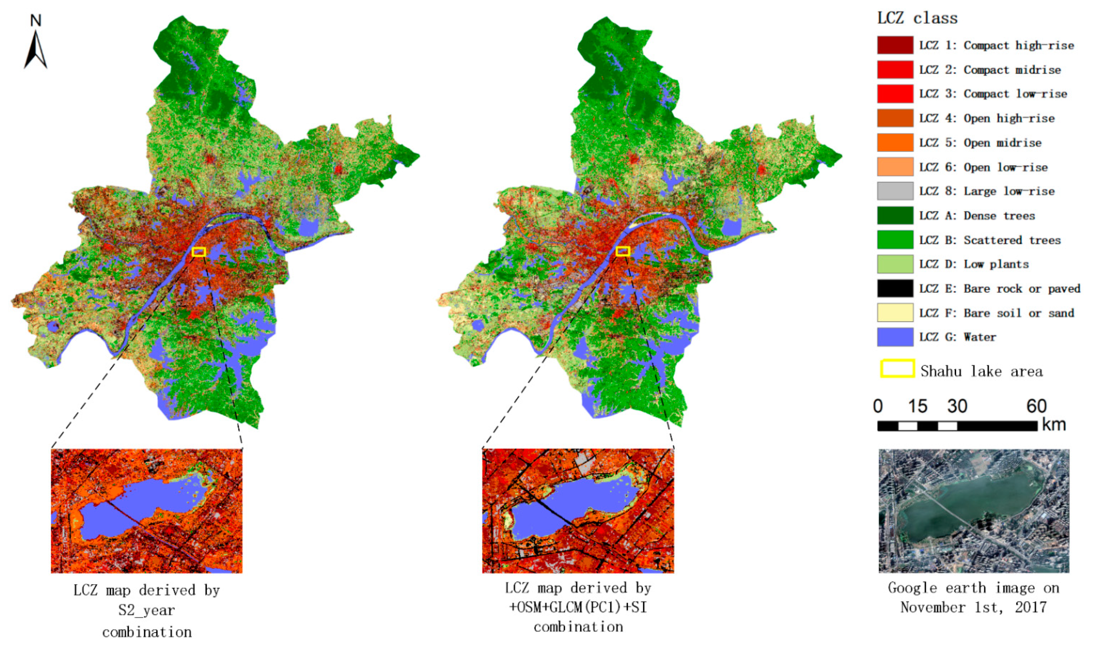
4.2. LCZ Map of Wuhan

In total, 19 LCZ maps of Wuhan were generated by 19 dataset combinations. +OSM+GLCM(PC1)+SI and S2_year combinations have the highest and lowest OA accuracy, respectively. Figure 6 compares the two LCZ classifications generated by +OSM+GLCM(PC1)+SI and S2_year combinations. It was found that: (1) most of built type LCZ classes were located in the urban center of Wuhan; (2) LCZ A (i.e., dense tree) are mainly located in the northwest of Wuhan; (3) LCZ B (i.e., scatter tree) mainly distributed in the northwest and south-east of Wuhan; (4) LCZ G (i.e., water) could be depicted accurately in LCZ classification as water is more separable from other LCZ classes. (5) To compare two LCZ maps in detail, we selected the Shahu Lake area to zoom in on these two maps and compare them based on the corresponding google earth image. LCZ E (i.e., paved) and LCZ G (i.e., water) on the +OSM+GLCM(PC1)+SI map were more accurate than that on the S2_year map. Built type LCZ classes were overestimated on the S2_year map to some degree. Even LCZ G (i.e., water) was classified as LCZ 4 (i.e., open high-rise) or LCZ 5 (i.e., open midrise). In contrast, built type LCZ classes on +OSM+GLCM(PC1)+SI map are more consistent with google earth image. That proved again that the +OSM+GLCM(PC1)+SI combination could generate a more accurate LCZ map.

5. Conclusions

Open data from Sentinel-2, Sentinel-1, OSM, GLCM, SI, and NTL were used to map the LCZ classes in Wuhan. These datasets were purposefully selected as offering different, but complementary information on the urban area and so could potentially be combined to produce an accurate LCZ map. The combination of seasonal optical and radar data from the Sentinel satellites provided a benchmark classification based on open data. The addition of secondary datasets to this combination could increase the accuracy of LCZ classifications. The OSM, GLCM, SI, and NTL datasets could be constructively combined with the Sentinel data. The highest OA value was obtained by using seasonal Sentinel-2 and Sentinel-1, OSM, and image texture datasets. Although more datasets would get a more accurate classification usually, it may not always be an absolutely effective way to improve the LCZ classification accuracy result by combining as many datasets as possible. This would have good guidance on data source selection for other study areas’ LCZ classification.

It may be possible to further enhance the LCZ mapping accuracy. For example, other ancillary datasets such as the point of interest data the social media (e.g., Sina Weibo or WeChat) check-in data may provide useful information to refine the mapping, especially concerning the built type LCZ classes. The latter were classified to a lower accuracy (OAb= 65.93%) than the land cover classes (OAlc = 88.06%). Most importantly, POI and social media check-in data also are open access for the public. The open and free datasets provide more possibilities for LCZ mapping in other cities. Not only the data source but also the classification method is a direction of effort. RF classifier is a powerful classifier in most image classifications. As the built type LCZ classes are hard to differentiate, the RF classifier did not get an ideal accuracy result for all built type LCZ classes. Hence, a more powerful classifier, such as the deep learning method, could be used in further study. Moreover, this study provides the potential to generate more accurate LCZ mapping on a large scale using the GEE platform, which is significant for urban development.

References

1. Taha, H. Urban climates and heat islands: Albedo, evapotranspiration, and anthropogenic heat. Energy Build. 1997, 25, 99–103. [Google Scholar] [CrossRef] [Green Version]
2. Oke, T.R. The energetic basis of the urban heat island. Q. J. R. Meteorol. Soc. 1982, 108, 1–24. [Google Scholar] [CrossRef]
3. Voogt, J.A.; Oke, T.R. Thermal remote sensing of urban climates. Remote Sens. Environ. 2003, 86, 370–384. [Google Scholar] [CrossRef]
4. Founda, D.; Santamouris, M. Synergies between Urban Heat Island and Heat Waves in Athens (Greece), during an extremely hot summer (2012). Sci. Rep. 2017, 7, 10973. [Google Scholar] [CrossRef] [PubMed] [Green Version]
5. Salata, F.; Golasi, I.; Petitti, D.; Vollaro, E.D.L.; Coppi, M.; Vollaro, A.D.L. Relating microclimate, human thermal comfort and health during heat waves: An analysis of heat island mitigation strategies through a case study in an urban outdoor environment. Sustain. Cities Soc. 2017, 30, 79–96. [Google Scholar] [CrossRef]
6. Yadav, N.; Sharma, C.; Peshin, S.K.; Masiwal, R. Study of intra-city urban heat island intensity and its influence on atmospheric chemistry and energy consumption in Delhi. Sustain. Cities Soc. 2017, 32, 202–211. [Google Scholar] [CrossRef]
7. Fallmann, J.; Forkel, R.; Emeis, S. Secondary effects of urban heat island mitigation measures on air quality. Atmos. Environ. 2016, 125, 199–211. [Google Scholar] [CrossRef] [Green Version]
8. Grimmond, S. Urbanization and global environmental change: Local effects of urban warming. Geogr. J. 2007, 173, 83–88. [Google Scholar] [CrossRef]
9. Stewart, I.D.; Oke, T.R. Local Climate Zones for Urban Temperature Studies. Bull. Am. Meteorol. Soc. 2012, 93, 1879–1900. [Google Scholar] [CrossRef]
10. Ching, J.; Mills, G.; Bechtel, B.; See, L.; Feddema, J.; Wang, X.; Ren, C.; Brousse, O.; Martilli, A.; Neophytou, M.; et al. WUDAPT: An Urban Weather, Climate, and Environmental Modeling Infrastructure for the Anthropocene. Bull. Am. Meteorol. Soc. 2018, 99, 1907–1924. [Google Scholar] [CrossRef] [Green Version]
11. Wang, R.; Ren, C.; Xu, Y.; Lau, K.K.-L.; Shi, Y. Mapping the local climate zones of urban areas by GIS-based and WUDAPT methods: A case study of Hong Kong. Urban Clim. 2018, 24, 567–576. [Google Scholar] [CrossRef]
12. Bechtel, B.; Alexander, P.J.; Beck, C.; Bohner, J.; Brousse, O.; Ching, J.; Demuzere, M.; Fonte, C.C.; Gal, T.; Hidalgo, J. Generating WUDAPT Level 0 data–Current status of production and evaluation. Urban Clim. 2019, 27, 24–45. [Google Scholar] [CrossRef] [Green Version]
13. Danylo, O.; See, L.; Bechtel, B.; Schepaschenko, D.; Fritz, S. Contributing to WUDAPT: A Local Climate Zone Classification of Two Cities in Ukraine. IEEE J. Sel. Top. Appl. Earth Obs. Remote Sens. 2016, 9, 1841–1853. [Google Scholar] [CrossRef] [Green Version]
14. Cai, M.; Ren, C.; Xu, Y.; Lau, K.K.-L.; Wang, R. Investigating the relationship between local climate zone and land surface temperature using an improved WUDAPT methodology—A case study of Yangtze River Delta, China. Urban Clim. 2018, 24, 485–502. [Google Scholar] [CrossRef]
15. Cai, M.; Ren, C.; Xu, Y.; Dai, W.; Wang, X.M. Local climate zone study for sustainable megacities development by using improved WUDAPT methodology–a case study in Guangzhou. Procedia Environ. Sci. 2016, 36, 82–89. [Google Scholar] [CrossRef] [Green Version]
16. Mills, G.; Ching, J.; See, L.; Bechtel, B.; Foley, M. An introduction to the WUDAPT project. In Proceedings of the 9th International Conference on Urban Climate, Toulouse, France, 20–24 July 2015; pp. 20–24. [Google Scholar]
17. Demuzere, M.; Bechtel, B.; Mills, G. Global transferability of local climate zone models. Urban Clim. 2019, 27, 46–63. [Google Scholar] [CrossRef]
18. Pradhesta, Y.F.; Nurjani, E.; Arijuddin, B.I. Local Climate Zone classification for climate-based urban planning using Landsat 8 Imagery (A case study in Yogyakarta Urban Area). In International Conference on Tropical Meteorology and Atmospheric Sciences; IOP Publishing: Bristol, UK, 2019; Volume 303. [Google Scholar]
19. Yue, Y.; Zhan, Q.; Wang, J.; Xiao, Y. Optimizing the urban thermal environment at local scale: A case study in Wuhan, China. Int. J. Sustain. Dev. Plan. 2017, 12, 1312–1325. [Google Scholar] [CrossRef] [Green Version]
20. Verdonck, M.L.; Okujeni, A.; van der Linden, S.; Demuzere, M.; De Wulf, R.; Van Coillie, F. Influence of neighbourhood information on ‘Local Climate Zone’ mapping in heterogeneous cities. Int. J. Appl. Earth Obs. Geoinf. 2017, 62, 102–113. [Google Scholar] [CrossRef]
21. Yoo, C.; Han, D.; Im, J.; Bechtel, B. Comparison between convolutional neural networks and random forest for local climate zone classification in mega urban areas using Landsat images. ISPRS J. Photogramm. Remote Sens. 2019, 157, 155–170. [Google Scholar] [CrossRef]
22. Xu, Y.; Ren, C.; Cai, M.; Edward, N.Y.Y.; Wu, T. Classification of Local Climate Zones Using ASTER and Landsat Data for High-Density Cities. IEEE J. Sel. Top. Appl. Earth Obs. Remote Sens. 2017, 10, 3397–3405. [Google Scholar] [CrossRef]
23. Qiu, C.; Schmitt, M.; Mou, L.; Ghamisi, P.; Zhu, X.X. Feature Importance Analysis for Local Climate Zone Classification Using a Residual Convolutional Neural Network with Multi-Source Datasets. Remote Sens. 2018, 10, 1572. [Google Scholar] [CrossRef] [Green Version]
24. Fonte, C.C.; Lopes, P.; See, L.; Bechtel, B. Using OpenStreetMap (OSM) to enhance the classification of local climate zones in the framework of WUDAPT. Urban Clim. 2019, 28, 100456. [Google Scholar] [CrossRef]
25. Geletič, J.; Lehnert, M. GIS-based delineation of local climate zones: The case of medium-sized Central European cities. Morav. Geogr. Rep. 2016, 24, 2–12. [Google Scholar] [CrossRef] [Green Version]
26. Hu, J.; Ghamisi, P.; Zhu, X.X. Feature extraction and selection of sentinel-1 dual-pol data for global-scale local climate zone classification. ISPRS Int. J. Geo-Inf. 2018, 7, 379. [Google Scholar] [CrossRef] [Green Version]
27. Bechtel, B.; See, L.; Mills, G.; Foley, M. Classification of Local Climate Zones Using SAR and Multispectral Data in an Arid Environment. IEEE J. Sel. Top. Appl. Earth Obs. Remote Sens. 2016, 9, 3097–3105. [Google Scholar] [CrossRef]
28. Reza, A.; Jalal, A.; Claudia, N.; Felix, G. Synergetic Use of Sentinel-1 and Sentinel-2 Data for Soil Moisture Mapping at Plot Scale. Remote Sens. 2018, 10, 1285. [Google Scholar]
29. Guo, J.; Lin, Z.; Jin, B. Crop Classification Based on Data Fusion of Sentinel-1 and Sentinel-2. Trans. Chin. Soc. Agric. Mach. 2018, 49, 192–198. [Google Scholar]
30. Wangchuk, S.; Bolch, T. Mapping of glacial lakes using Sentinel-1 and Sentinel-2 data and a random forest classifier: Strengths and challenges. Sci. Remote Sens. 2020, 2, 100008. [Google Scholar] [CrossRef]
31. Kaplan, G.; Avdan, U. Sentinel-1 and sentinel-2 data fusion for wetlands mapping: Balikdami, turkey. Int. Arch. Photogramm. Remote. Sens. Spat. Inf. Sci. 2018, 42. Available online: https://d-nb.info/1161190805/34 (accessed on 1 May 2020). [CrossRef] [Green Version]
32. Gorelick, N.; Hancher, M.; Dixon, M.; Ilyushchenko, S.; Moore, R. Google Earth Engine: Planetary-scale geospatial analysis for everyone. Remote Sens. Environ. 2017, 202, 18–27. [Google Scholar] [CrossRef]
33. Blaes, X.; Vanhalle, L.; Defourny, P. Efficiency of crop identification based on optical and SAR image time series. Remote Sens. Environ. 2005, 96, 352–365. [Google Scholar] [CrossRef]
34. Werner, A.; Storie, C.D.; Storie, J. Evaluating SAR-Optical Image Fusions for Urban LULC Classification in Vancouver Canada. Can. J. Remote Sens. 2014, 40, 278–290. [Google Scholar] [CrossRef]
35. Qiu, C.; Mou, L.; Schmitt, M.; Zhu, X.X. Local climate zone-based urban land cover classification from multi-seasonal Sentinel-2 images with a recurrent residual network. ISPRS J. Photogramm. Remote Sens. 2019, 154, 151–162. [Google Scholar] [CrossRef] [PubMed]
36. Zhu, Z.; Wang, S.; Woodcock, C.E. Improvement and expansion of the Fmask algorithm: Cloud, cloud shadow, and snow detection for Landsats 4–7, 8, and Sentinel 2 images. Remote Sens. Environ. 2015, 159, 269–277. [Google Scholar] [CrossRef]
37. Phan, T.N.; Kuch, V.; Lehnert, L.W. Land Cover Classification using Google Earth Engine and Random Forest Classifier—The Role of Image Composition. Remote Sens. 2020, 12, 2411. [Google Scholar] [CrossRef]
38. Tucker, C.J. Red and photographic infrared linear combinations for monitoring vegetation. Remote Sens. Environ. 1979, 8, 127–150. [Google Scholar] [CrossRef] [Green Version]
39. McFeeters, S.K. The use of the Normalized Difference Water Index (NDWI) in the delineation of open water features. Int. J. Remote Sens. 1996, 17, 1425–1432. [Google Scholar] [CrossRef]
40. Haralick, R.M.; Shanmugam, K.; Dinstein, I. Textural Features for Image Classification. IEEE Trans. Syst. Manand Cybern. 1973, 3, 610–621. [Google Scholar] [CrossRef] [Green Version]
41. Conners, R.W.; Trivedi, M.M.; Harlow, C.A. Segmentation of a high-resolution urban scene using texture operators. Comput. Vis. Graph. Image Process. 1984, 25, 273–310. [Google Scholar] [CrossRef]
42. Haklay, M.; Weber, P. OpenStreetMap: User-Generated Street Maps. IEEE Pervasive Comput. 2008, 7, 12–18. [Google Scholar] [CrossRef] [Green Version]
43. Li, X.; Zhao, L.; Li, D.; Xu, H. Mapping Urban Extent Using Luojia 1-01 Nighttime Light Imagery. Sensors 2018, 18, 3665. [Google Scholar] [CrossRef] [PubMed] [Green Version]
44. Ren, C.; Cai, M.; Li, X.; Zhang, L.; Ng, E. Assessment of Local Climate Zone Classification Maps of Cities in China and Feasible Refinements. Sci. Rep. 2019, 9, 1–11. [Google Scholar] [CrossRef] [PubMed] [Green Version]
Figure 1. The study area of Wuhan.
Land 10 00454 g001
Figure 2. A sample of Sentinel-2 data and the sample location is Shahu Lake, Wuhan. The false-color composite multispectral images: Red: B8; Green: B4; Blue: B3 were shown.
Land 10 00454 g002
Figure 3. A sample of Sentinel-1 data. The grayscale images of the VV band were shown.
Land 10 00454 g003
Figure 4. A sample of the OSM data.
Land 10 00454 g004
Figure 5. A sample of the Luojia1-01 data.
Land 10 00454 g005
Figure 6. The LCZ map of Wuhan City.
Land 10 00454 g006